Evaluating extensions to LCDM: an application of Bayesian model averaging

Abstract

We employ Bayesian Model Averaging (BMA) as a powerful statistical framework to address key cosmological questions about the universe’s fundamental properties. We explore extensions beyond the standard $\Lambda$CDM model, considering a varying curvature density parameter $\Omega_{\rm{K}}$, a spectral index $n_{\rm{s}}$$=1$ and a varying $n_{\rm{run}}$, a constant dark energy equation of state (EOS) $w_{\rm{0}}$CDM and a time-dependent one $w_{\rm{0}}$$w_{\rm{a}}$CDM. We also test cosmological data against a varying effective number of neutrino species $N_{\rm{eff}}$. Data from different combinations of cosmic microwave background (CMB) data from the last Planck PR4 analysis, CMB lensing from Planck 2018, baryonic acoustic oscillations (BAO) and the Bicep-KECK 2018 results, are used. We find that the standard $\Lambda$CDM model is favoured when combining CMB data with CMB lensing, BAO and Bicep-KECK 2018 data against K-$\Lambda$CDM model $N_{\rm{eff}}$-$\Lambda$CDM with a probability $>80\%$. When investigating the dark energy EOS, we find that this dataset is not able to express a strong preference between the standard $\Lambda$CDM model and the constant dark energy EOS model $w_{\rm{0}}$CDM, with an approximately split model posterior probability of $\approx 60\%:40\%$ in favour of $\Lambda$CDM  whereas the time-varying dark energy EOS model is ruled out. Finally, we find that the CMB data alone show a strong preference for a model that includes the running of the spectral index $n_{\rm{run}}$, with a probability $\approx 90\%$, when compared to the $n_{\rm s}=1$ model and the standard $\Lambda$CDM. Overall, we find that including the model uncertainty in the considered cases does not significantly impact the Hubble tension.

1 Introduction

The $\Lambda$CDM cosmological model has been the prevailing paradigm for the last 25 years, successfully encapsulating the large-scale structure and evolution of the Universe in a model with a relatively small number of parameters ([1, 2] and refs therein). However, as our observational capabilities have advanced, a nuanced exploration of the model’s foundations has become imperative. Bayesian Model Averaging (BMA) is a robust statistical framework for comparing alternative models, allowing for a comprehensive assessment of various cosmological extensions [3]. We investigate the applications of BMA within the context of the $\Lambda$CDM model, employing chain post-processing methodologies as presented by [4] to rigorously evaluate the model posterior probabilities associated with key extensions.

We focus on four possible extensions to the $\Lambda$CDM model: (1) the introduction of a dynamical dark energy component, parameterized by the equation-of-state $w(z)$; (2) the inclusion of spatial curvature, characterized by the parameter $k$; (3) variations in the primordial power spectrum, encapsulated by the power law index $n_{s}(k)$; and (4) an additional neutrino species. Each of these extensions has distinct implications for the cosmic evolution and structure formation, necessitating a careful examination of their likelihood within the observational constraints. The inclusion of spatial curvature is motivated by both theoretical considerations and observational hints, prompting a reevaluation of the universe’s global geometry [2]. Dark energy, represented by its equation of state, remains a key driver of cosmic acceleration, and probing its potential evolution introduces an additional layer of complexity [5]. The running of the spectral index introduces a departure from the scale invariance of primordial density fluctuations, while the presence of tensor modes directly relates to the elusive gravitational wave background from cosmic inflation.

To tackle this multifaceted exploration, we adopt the chain post-processing techniques outlined in [4]. This provides a systematic and computationally efficient means of extracting precise model posterior probabilities from cosmological parameter chains generated through Markov Chain Monte Carlo (MCMC) simulations for individual model choices. By applying these techniques to extended $\Lambda$CDM scenarios, we aim to obtain a nuanced understanding of the statistical evidence and viability of each model within the Bayesian framework. The four possible extensions discussed above are tested using the following model comparisons: (1) $\Lambda$CDM, and $w_{\rm{0}}$CDM which considers a varying equation-of-state (parameterized by $w_{\rm{0}}$), and $w_{\rm{0}}$$w_{\rm{a}}$CDM with both $w_{\rm{0}}$ and a time-varying parameter $w_{\rm{a}}$; (2) $\Lambda$CDM  and $k$$\Lambda$CDM with spatial curvature $k$; (3) $\Lambda$CDM  and $\Lambda$CDM with a fixed spectral index—corresponding to a Harrison-Zeldovich power spectrum (hereon HZ) with $n_{\rm{s}}$$=1$—and $\Lambda$CDM with a running spectral index, commonly denoted as $n_{\rm{run}}$$\,=\,$$\mathrm{d}n_{\mathrm{s}}/\mathrm{d}\ln k$; and (4), we test the $\Lambda$CDM model against a varying number of neutrino species $N_{\rm eff}$.

In undertaking this research, we align with the growing body of literature that recognizes the importance of sophisticated statistical methods when confronting the complexities of modern cosmological data [6, 7, 4]. This work proposes a step towards refining our cosmological framework, ensuring that our understanding of the universe remains aligned with the latest observational evidence.

As well as allowing us to assign probabilities to models, BMA also provides a mechanism for deriving credible intervals for cosmological parameters common to multiple models, when marginalising over the model choice. Thus, for example, we can show how the estimate of the Hubble parameter today, $\rm H_{0}$, changes according to the additional model uncertainty. For the Hubble parameter, this is particularly interesting given the ”Hubble tension”, where incompatible measurements have been made using different techniques. The CMB data reported a value of $H_{0}$ close to $68$kms^-1Mpc^-1 for $\Lambda$CDM cosmologies [2]. This is supported by the combination of observations of Baryon Acoustic Oscillation (BAO) from the Sloan Digital Sky Survey (SDSS) and Big Bang Nucleosynthesis (BBN) constraints, which favour similar values for the same models [8]. In contrast, observations from local distance ladder studies, such as the Hubble Space Telescope (HST) observations of Cepheid variable stars, favour a higher value of $H_{0}\sim 74$kms^-1Mpc^-1 [9]. We consider how the error on $H_{0}$ varies when marginalised over the extensions to the $\Lambda$CDM model listed above. We find increased credible intervals, in line with other analyses [10, 11, 12, 13], but that such extensions do not solve the problem [14]. The extension of BMA to Early Dark Energy models, designed to solve this tension was considered in [4].

The structure of this paper is as follows: In Sect. 2 we summarize the BMA methodology and implementation. We then show our results by considering different combinations of cosmological models in Sect. 3. In Sect. 4 we conclude with a comment on our findings and future perspectives about the application of BMA to model selection in Cosmology.

2 Bayesian Model Averaging

Bayesian Model Averaging (BMA) offers a principled approach to deal with the choice of various cosmological models. At the heart of BMA lies a departure from the conventional model selection paradigm, rather than choosing a single best model, and then considering parameters within that model, one can instead jointly consider a number of models and the weighted prediction for common parameters. In essence, model choice simply becomes a discrete parameter to be constrained or marginalised over. By assigning posterior probabilities to a set of candidate models based on the observed data, BMA combines predictions from each model, weighting them according to their posterior model posterior probabilities. This results in a comprehensive and nuanced representation of the uncertainty associated with model choice, fostering a robust and accurate inference process.

BMA differs from conventional manual or automatic post-hoc selection strategies based on goodness of fit measures likeAkaike Information Criterion (AIC)[15]. Such methods focus on identifying a single optimal model, neglecting the fact that there is uncertainty in this choice much like uncertainty in parameter estimates (see for instance [16]). BMA, with its probabilistic framework, provides a more inclusive approach by considering a range of models, thus offering a more realistic reflection of the underlying uncertainty. Another possible approach are cross-validation methods [17]. While valuable for assessing model performance, these may not explicitly address model uncertainty. BMA, on the other hand, explicitly incorporates uncertainty through probabilistic model averaging, allowing for a more nuanced understanding of the uncertainty associated with parameter estimates and predictions.

To see how BMA and the approach of [4] work, let $M=1,2,...,K$ be a discrete random variable indicating a choice among $K$ different models. For convenience, we will refer to $M=j$ as $M_{j}$. The posterior model posterior probability for model $M_{\rm{i}}$, denoted as $P(M_{\rm{i}}|\vec{d})$, is computed as

$$P(M_{\rm{i}}|\vec{d})=\frac{P(M_{\rm{i}})P(\vec{d}|M_{\rm{i}})}{\sum_{\rm{j}=1}^{\rm{K}}P(M_{\rm{j}})P(\vec{d}|M_{\rm{j}})}\,,$$ (2.1)

where $P(M_{\rm{i}})$ is the prior probability of model $M_{\rm{i}}$, $P(\vec{d}|M_{\rm{i}})$ is the marginal likelihood of the data $\vec{d}$ given model $M_{\rm{i}}$, and the denominator serves as a normalization factor to ensure that the probabilities sum to one. We assume that the prior probabilities are separable between model selection and model parameters. Given the model posterior probability $P(M_{\rm{i}}|\vec{d})$, we can marginalize over the model uncertainty and compute the model parameters’ posterior distribution as:

$$P(\vec{\theta}|\vec{d})=\sum_{i=1}^{K}P(\vec{\theta},M_{i}|\vec{d})=\sum_{i=1}^{K}P(\vec{\theta}|\vec{d},M_{i})P(M_{i}|\vec{d})\,.$$ (2.2)

Since samples of $P(\vec{\theta}|\vec{d},M_{1})$ and $P(\vec{\theta}|\vec{d},M_{2})$ are readily available from standard analyses conditional on a single model, it then only remains to obtain the two model posteriors $P(M_{\rm{i}}|\vec{d})$ defined in Eq. 2.1. This decomposition frames the model-averaged posterior $P(\vec{\theta}|d)$ as the weighted average of the model-conditional posteriors $P(\vec{\theta}|\vec{d},M_{i})$ as in Eq. 2.2. Note that it is not sufficient to weight by the model-priors $P(M_{i})$; rather the weights correspond to the model posteriors $P(M_{i}|\vec{d})$ via a suitable estimator (see, [18, 4]):

$$\hat{P}(\vec{d}|M_{\rm{i}})=\frac{\rm{N}_{\rm{i}}}{\sum_{\rm{t}=1}^{\rm{N}_{\rm{i}}}\left[1/P(\vec{d}|M_{\rm{i}},\vec{\theta}_{\rm{i}}^{(\rm{t})})\right]}\,.$$ (2.3)

The data themselves inform how much weight is assigned to either model. We therefore applied BMA by importance sampling existing model conditional chains [19]. This methodology has been implemented for cosmological analyses in [4], and referred as Fast-MPC. Details of the implementation can be found in [4]. Briefly, one can apply BMA to existing chains as follows:

1. Fit candidate models: run two or more MCMC chains assuming model $M_{i}$, yielding $\{\vec{\theta}_{i}\}_{\rm{N}_{i}}$, $\{P(\vec{d}|M_{\rm{i}},\vec{\theta}_{\rm{i}})\}_{\rm{N}_{i}}$.

2. Estimate ${P}(\vec{d}|M_{i})$: compute estimates $\hat{P}(\vec{d}|M_{i})$ via Eq. 2.3.

3. Estimate model posteriors: substitute estimates $\hat{P}(\vec{d}|M_{i})$ into Eq. 2.1 to estimate $P(M_{i}|d)$.

4. Estimate marginal (model-averaged) posteriors of $\vec{\theta}$: substitute estimates of $P(M_{i}|d)$ into Eq. 2.2.

3 Model choices in cosmology

For our analysis, we considered the following combination of $\Lambda$CDM base parameters with flat prior ranges, unless otherwise specified: the present day value of the Hubble parameter $\rm H_{0}\in[20,100]$, the baryon density parameter $\Omega_{\rm{b}}\rm{h}^{2}\in[0.005,0.1]$, the cold dark matter density parameter $\Omega_{\rm{c}}\rm{h}^{2}\in[0.001,0.99]$, the amplitude of scalar perturbations $\log(10^{10}A_{\mathrm{s}})\in[1.61,3.91]$, the index of the scalar perturbations $n_{\rm{s}}\in[0.8,1.2]$ and the optical depth of reionization $\tau\in[0.01,0.8]$. In addition, we include the following $\Lambda$CDM extensions when considering the respective extended $\Lambda$CDM model: the curvature density parameter $\Omega_{\rm k}\in[-0.3,0.3]$, the DE EOS parameters $w_{\rm{0}}$$\,\in[-3,0.3]$ and $w_{\rm{a}}$$\,\in[-3,2]$, the running of the primordial fluctuations spectral index $n_{\rm{run}}$$\,\in[-0.02,0.01]$ and the effective number of neutrino species $N_{\rm{eff}}$$\,\in[2,4]$.

As a fully Bayesian technique, BMA requires us to assign a prior probability to our models; we explore, as a default assumption, a flat or uniform prior, consisting of equal prior probability, $P(M_{\rm i})$ in Eq. 2.1, to each candidate model.

3.1 Dataset

In this work, we include the following datasets:

• CMB: the full Planck low-$\ell$ and high-$\ell$ likelihood as presented in [20]. This analysis was based on the publicly available codes lollipop, covering CMB polarization E and B low-$\ell$ modes in $2\leq\ell\leq 30$, and hillipop, that includes the CMB TT, TE and EE multipoles in $30<\ell\leq 2500$. The TT multipoles in $2\leq\ell\leq 30$ are included through the commander Planck 2018 likelihood [21], based on a gaussianized Blackwell-Rao estimator on the full-sky CMB power spectra from component-spearated CMB maps.

• Lensing: Planck 2018 reconstructed CMB lensing potential power spectrum [22].

• BAO: Baryon Acoustic Oscillation measurements from SDSS DR7 main galaxy sample [23] at $z=0.15$, the updated BAO reconstruction from 6dF galaxy redshift survey [24] at $z=0.097$ and the BOSS DR12 [25] LOWZ and CMASS galaxy samples at $z=0.38$, $z=0.51$ and $z=0.61$, the eBOSS galaxies and quasars in $0.6\leq z\leq 2.2$ [26], and the Lyman-$\alpha$ forest samples in $1.8\leq z\leq 3.5$.

• BK18: the Bicep-Keck array CMB polarization data from the 2018 observing season [27].

The MCMC runs have been carried out with the publicly available software cobaya [28, 29]. The resulting chains have been initially analysed with the public code getdidst [30], and then post-processed with fast-mpc [4].

3.2 Application 1: Is the Universe flat?

The first open question about the Cosmological model we address is the one concerning the curvature. While the standard $\Lambda$CDM model is based on a flat Universe with $\Omega_{\rm k}=0$, CMB data showed a tension with this when $\Omega_{\rm{K}}$ was included in the analysis of previous Planck data [31, 2, 32]. This tension has been drastically reduced to $\lesssim 1\sigma$ with the most recent Planck PR4 data reanalysis from [20], and removed completely when CMB data are combined with BAO, as shown in the same paper.

We now present the results of BMA including both the flat $\Lambda$CDM model, and the curved K-$\Lambda$CDM. For this analysis we considered two dataset configurations: CMB alone and a combination of CMB, CMB lensing, BAO and BK18. We report in Tab. 1 the probabilities associated to the two considered models under a flat model prior assumption and for the two considered datasets; in the flat prior assumption, the CMB data alone suggest a quasi-split model posterior probability (57% and 43% for $\Lambda$CDM and K-$\Lambda$CDM  respectively), whereas the flat $\Lambda$CDM model is favoured with a 88% probability when CMB is combined with lensing, BAO and BK18. We show the model posterior probabilities for different model prior choices in Fig. 6 for CMB alone (red line), and for CMB+lens+BAO+BK18 (green line); in the first case we highlight how the model posterior probability follows the prior choice, indicating a poor model constraining power of the CMB dataset alone.

Dataset	$\Lambda$CDM	K-$\Lambda$CDM
CMB	$57.0\%$	$43.0\%$
CMB+lens+BAO+BK18	$88.0\%$	$12.0\%$

Table 1: Model posterior probabilities for the $\Lambda$CDM and K-$\Lambda$CDM under a flat model prior assumption. We compare the CMB dataset alone and including lensing, BAO and Bicep-KECK 2018 results.

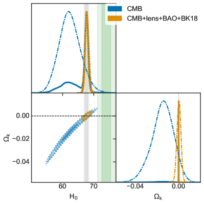
Figure 1: Posterior distribution in the $\Omega_{\rm k}-\rm{H}_{0}$ parameter space. Solid lines show the model-marginalized constraints with a flat model prior assumption, dotted lines report the $\Lambda$CDM model conditionals and dot-dashed ones the K-$\Lambda$CDM model conditionals. We included as vertical bands the the constraint (68% and 95% CL) on $H_{0}$ from Planck 2018 [2] (gray), and from SNIa [9] (green), both under the $\Lambda$CDM model assumption.

We present in Fig. 5 the marginalized constraints on the 6 $\Lambda$CDM base parameters (brown and purple lines); we also show in Fig. 1 a focus on the the $\Omega_{\rm k}-\rm{H}_{0}$ degeneracy in the BMA context, after marginalizing over the model uncertainty associated to the probabilities of the standard $\Lambda$CDM and the extended K-$\Lambda$CDM. In the latter figure we notice how a curvature parameter preference for negative values leads to smaller preferred values of the Hubble parameter, in the opposite direction with respect to solving the Hubble tension. The constraint on $\rm H_{0}$, after marginalizing over model uncertainty, are:

$$\rm{CMB} \rm H_{0}=65.3^{+3.6}_{-4.6}$$ (3.1)

$$\rm{CMB+lens+BAO+BK18} \rm H_{0}=67.73\pm 0.49$$ (3.2)

The CMB estimate is about $0.13\sigma$ below the mean value from the $\Lambda$CDM-conditional value $67.36\pm 0.61$, and $0.18\sigma$ above the K-$\Lambda$CDM conditional value of $\rm H_{0}=62.3^{+3.2}_{-3.6}$, as expressed in units of the model marginal estimate’s standard deviation; however, the main impact of marginalizing over the model uncertainty is in the increase of the total uncertainty on $\rm H_{0}$ of $\frac{\sigma_{\rm marg}-\sigma_{\rm cond}}{\sigma_{\rm cond}}\approx 10$. The CMB+lens+BAO+BK18, on the other hand, is fully consistent with the $\Lambda$CDM-conditional value $67.67\pm 0.42$, with a $\approx 16\%$ increase in the parameter estimate’s uncertainty. Similarly, we found the estimates of the curvature density $\Omega_{\rm{K}}$ after marginalizing over the model uncertainty to be:

$$\rm{CMB} \Omega_{\rm k}=-0.0067^{+0.0069}_{-0.013}$$ (3.3)

$$\rm{CMB+lens+BAO+BK18} \Omega_{\rm k}=0.00007^{+0.00097}_{-0.00015}$$ (3.4)

Both the estimates are fully compatible with a flat Universe within $1\sigma$, despite the uncertainty on $\rm H_{0}$ from CMB alone being $\approx 50\%$ smaller than the K-$\Lambda$CDM conditional estimate $\Omega_{\rm k}=-0.0148^{+0.011}_{-0.0088}$ because the posterior is now skewed in the right direction thanks to the BMA. The full dataset case shows instead a much more consistent estimate of $\Omega_{\rm k}$ with respect to the K-$\Lambda$CDM model conditional one $\Omega_{\rm k}=-0.0002\pm 0018$.

3.3 Application 2: Is the Dark Energy EOS $w=-1$?

Dark energy contributes  70% of the Universe’s total energy density, and it is responsible for the accelerated expansion of the cosmos [33, 34]. The parameterization of dark energy equation of state provides a versatile framework for understanding its evolution. In this context, although not related to a physical model, the parameters $w_{\rm{0}}$ and $w_{\rm{a}}$ offer valuable insights into the present-day behaviour and the redshift-dependent evolution of dark energy. In this section, we apply BMA to compare three different models: 1) the standard $\Lambda$CDM, that considers a constant energy density term $\Omega_{\Lambda}$; 2) a DE EOS with a constant pressure term $w=w_{0}$; and 3) a time-varying DE EOS $w=w_{0}+w_{a\rm}(1-a)$.

We only consider the most constraining dataset including CMB, CMB lensing, BAO and BK18; we did not include also type Ia Supernovae in our analysis, following [2] in order to avoid the $\rm H_{0}$ tension, and focus our model comparison on DE only. We show in Tab. 2 the different model posterior probabilities, with a flat model prior assumption. These show a mild preference for the standard $\Lambda$CDM model, as compared to the minimal constant EOS $w_{\rm{0}}$CDM model; the most complex $w_{\rm{0}}$$w_{\rm{a}}$CDM is instead highly discouraged with a relative probability below $\sim$1%.

Dataset	$\Lambda$CDM	$w_{\rm{0}}$CDM	$w_{\rm{0}}$$w_{\rm{a}}$CDM
CMB+lens+BAO+BK18	$59.5\%$	$39.9\%$	$0.6\%$

Table 2: Model posterior probabilities for the $\Lambda$CDM model, the minimal DE EOS extension $w_{\rm{0}}$CDM and the more complex $w_{\rm{0}}$$w_{\rm{a}}$CDM under a flat model prior assumption.

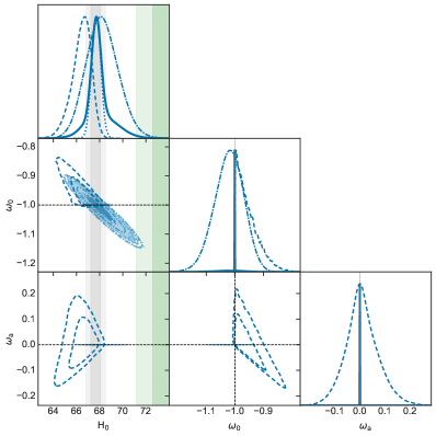
Figure 2: Posterior distributions in the $\rm H_{0}$-$w_{\rm{0}}$$w_{\rm{a}}$ parameter space. Solid lines show the model-marginalized constraints with a flat model prior assumption, dotted lines the $\Lambda$CDM ones, dot-dashed the posterior when assuming the $w_{\rm{0}}$CDM model, and dashed lines refer to the assumption of the $w_{\rm{0}}$$w_{\rm{a}}$CDM model. We included as vertical (horizontal) bands the the constraint (68% and 95% CL) on $H_{0}$ from Planck 2018 [2] (gray), and from SNIa [9] (green), both under the $\Lambda$CDM model assumption.

Marginalized cosmological parameters are shown in Fig. 5 (dark brown lines) for the base 6 parameters, while Fig. 2 focuses on the full $\rm H_{0}$-$w_{\rm{0}}$-$w_{\rm{a}}$ parameter space. We find that the 68% credible intervals on these parameters, after including the contribution from the model uncertainty, are:

$$\rm H_{0}=67.93^{+0.52}_{-0.91}$$ (3.5)

$$w_{\rm 0}=-1.009^{+0.011}_{-0.028}$$ (3.6)

$$w_{\rm a}=0.0001\pm 0.0053$$ (3.7)

The model-marginalized posterior distribution of $\rm H_{0}$ has a higher mean, and a slight skewness towards smaller values, However, the higher value of Hubble parameter, together with the $\approx 6\%$ larger uncertainty, still do not mitigate the Hubble tension in a significant way. Moreover, the model-marginalized estimates of both $w_{\rm{0}}$ and $w_{\rm{a}}$ show a strong compatibility with a constant dark energy EOS with $w_{0}=-1$.

3.4 Application 3: Is the Inflationary scalar spectral index $n_{s}=1$?

The primordial power spectrum represents the amplitude of density perturbations as a function of their spatial scale. It is generally assumed to have originated from quantum fluctuations during the inflationary epoch ([35, 36]). In this work we focus on the primordial power spectrum index $n_{\rm{s}}$, which describes the scale dependence of the amplitude of density fluctuations. A scale-invariant spectrum would have $n_{\rm s}=1$, meaning that the amplitude of perturbations is the same at all scales. However, CMB observations combined with CMB lensing and BAO showed a slightly lower value of $n_{\rm{s}}$ in the $\Lambda$CDM model of $n_{\rm s}=0.9665\pm 0.0038$ [2]. Additionally, the running of the spectral index, $n_{\rm{run}}$, where $k$ is the wavenumber, is a parameter that characterizes how $n_{\rm{s}}$ changes with scale. A non-zero $n_{\rm{run}}$ implies a scale dependence of the spectral index. While the $\Lambda$CDM model assumes a nearly scale-invariant spectrum, the possibility of a running spectral index is still explored in theoretical and observational studies. The current constraints on $n_{\rm{run}}$ from observations are consistent with zero within the measurement uncertainties [2].

We explore here three models: 1) the standard $\Lambda$CDM model with $n_{\rm{s}}$ free to vary in its prior range; 2) an Harrison-Zeldovich primordial power spectrum, corresponding to $n_{\rm s}=1$; and 3) an extended model that has $n_{\rm{s}}$ free and allows for the running of the spectral index $n_{\rm{run}}$. We computed the relative model posterior probabilities through BMA on a CMB-only dataset, and report our results in Tab. 3. The Harrison-Zeldovich model is completely discouraged, with a 0% probability; besides, the standard $\Lambda$CDM model only accounts for a  7% probability, and the $n_{\rm{run}}$ extension is favoured with a probability of  93%.

Dataset	$\Lambda$CDM	HZ-$\Lambda$CDM	$n_{\rm{run}}$-$\Lambda$CDM
CMB	$6.6\%$	$0\%$	$93.4\%$

Table 3: Model posterior probabilities for the $\Lambda$CDM model, the Harrison-Zeldovich HZ-$\Lambda$CDM and the $n_{\rm{run}}$-$\Lambda$CDM under a flat model prior assumption.

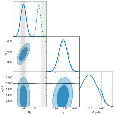
Figure 3: Posterior distribution in the $\rm H_{0}$-$n_{\rm{s}}$-$n_{\rm{run}}$ space. Solid lines report the model-marginalized constraints with a flat model-prior assumption, dotted lines the $\Lambda$CDM ones, dashed the HZ-$\Lambda$CDM and dot-dashed lines refer to the $n_{\rm{run}}$-$\Lambda$CDM model. The vertical grey band reports the the constraint (68% and 95% CL) on $H_{0}$ from Planck 2018 [2], and from SNIa [9] (green), under the $\Lambda$CDM model assumption.

The 6 base $\Lambda$CDM parameters marginalized over the model uncertainty are shown in Fig. 5 (green lines). We also show in Fig. 3 the $\rm H_{0}$-$n_{\rm{s}}$-$n_{\rm{run}}$ triangle plot. Marginalizing over the model uncertainty led to updated estimates of these parameters:

$$\rm H_{0}=67.73\pm 0.53$$ (3.8)

$$n_{\rm s}=0.9678\pm 0.0043$$ (3.9)

$$dn_{\rm s}/\mathrm{d}logk=-0.0094^{+0.0044}_{-0.0087}$$ (3.10)

We find a value of $\rm H_{0}$ only $\approx 0.7\sigma$ larger than the $\Lambda$CDM model conditional one, with $\approx 13\%$ smaller uncertainty. This is somewhat surprising if we think that we are considering more parameters than the standard $\Lambda$CDM model; however, BMA weights models according to their relative model posterior probabilities, and in this case we have a very strong preference for the more complex $n_{\rm{run}}$-$\Lambda$CDM model, which leads to a tighter constraint on $\rm H_{0}$. It is worth pointing out two additional aspects: in the context of the Hubble tension, the HZ model conditional constraint on $\rm H_{0}$, from CMB data alone, is $\rm H_{0}=70.73\pm 0.38$, approximately $\approx 3\sigma$ away from the SNIa measurement, although this model is ruled-out by the same data in our BMA analysis. Secondly, our BMA analysis shows that CMB data preference for a negative value of $n_{\rm{run}}$, at a $\approx 2\sigma$ level.

3.5 Application 4: How many neutrino species?

The standard cosmological model assumes a number of relativistic degrees of freedom for neutrinos, $N_{\rm{eff}}$$\,\approx 3.046$, slightly larger than 3 to account for the imperfect decoupling at electron-positron annihilation of the neutrino species [37, 38, 39]. This parameter can conveniently accommodate any non-interacting, non-decaying, massless particle produced long before recombination; it is defined so that the total relativistic energy density well after electron-positron annihilation is given by:

$$\rho_{\rm{rad}}=N_{\rm{eff}}\frac{7}{8}\left(\frac{4}{11}\right)^{4/3}\rho_{\gamma}$$ (3.11)

where $\rho_{\gamma}$ is the photon density. The most updated limits on this quantity comes from a combination of CMB, type Ia Supernovae, BAO and Large Scale Structure data ([40, 41].

In this work, we consider CMB alone and the combination of CMB, CMB lensing, BAO and BK18 to assess through BMA the relative model posterior probability of the $\Lambda$CDM standard model, and the $N_{\rm{eff}}$-$\Lambda$CDM model that accounts for additional relativistic species. We report the model posterior probabilities for the two datasets in Tab. 4 for a flat model prior, and illustrate the prior dependence in Fig. 6 for the CMB alone (blue line) and CMB+lens+BAO+BK18 (purple line). The CMB data alone highly encourage the extended $N_{\rm{eff}}$-$\Lambda$CDM model with a probability of  83% (with flat model prior), but standard $\Lambda$CDM is favoured when including lensing, BAO and the BK18 data, with a model posterior probability of  94%.

Dataset	$\Lambda$CDM	$N_{\rm{eff}}$-$\Lambda$CDM
CMB	$16.8\%$	$83.2\%$
CMB+lens+BAO+BK18	$94.4\%$	$5.6\%$

Table 4: Model posterior probabilities for the $\Lambda$CDM and $N_{\rm{eff}}$-$\Lambda$CDM under a flat model prior assumption. We compare the CMB dataset alone and including lensing, BAO and Bicep-KECK 2018 results.

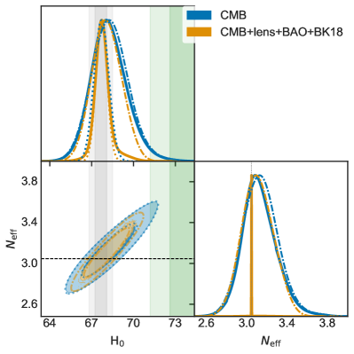
Figure 4: Posterior distributions in the $\rm H_{0}$-$N_{\rm{eff}}$parameters space; solid lines report the model-marginalized constraints with a flat model prior assumption, dotted lines refer to $\Lambda$CDM model-conditional ones and dash-dotted lines show the $N_{\rm{eff}}$-$\Lambda$CDM model-conditional constraints. Model posterior probabilities for the $\Lambda$CDM model against the $N_{\rm{eff}}$-$\Lambda$CDM model under a flat model prior assumption. We included as vertical bands the the constraint (68% and 95% CL) on $H_{0}$ from Planck 2018 [2] (gray), and from SNIa [9] (green), both under the $\Lambda$CDM model assumption.

As we did for the other model comparison in this paper, we propagate the model uncertainties to the 6 base parameters of the $\Lambda$CDM model common to all its extensions, and show the marginalized posterior distributions as orange and blue lines in Fig. 5. We present a focus on the $\rm H_{0}$-$N_{\rm{eff}}$parameters space in Fig. 4. We find the model-marginalized constraints on $\rm H_{0}$:

$$\rm{CMB} \rm H_{0}=68.3^{+1.1}_{-1.4}$$ (3.12)

$$\rm{CMB+lens+BAO+BK18} \rm H_{0}=67.79^{+0.41}_{-0.57}$$ (3.13)

For both the datasets, the marginalization over the model uncertainty when considering additional relativistic degrees of freedom through $N_{\rm{eff}}$ drives $\rm H_{0}$ in the right direction to solve the Hubble tension. Specifically, we find that the CMB data alone give a $0.8\sigma$ higher Hubble parameter estimate, with a $\approx 118\%$ larger uncertainty as compared to the $\Lambda$CDM model-conditional value; this value is driven by the high model posterior probability associated to the $N_{\rm{eff}}$-$\Lambda$CDM model when CMB data are considered alone –the Hubble parameter value is indeed the same as estimated in the $N_{\rm{eff}}$-$\Lambda$CDM model-conditional case. For the more extensive dataset, we recover a value of $\rm H_{0}$ closer to the $\Lambda$CDMconditional one, $\approx 0.3\sigma$ higher and with a standard deviation $\approx 9\%$ larger than the $\Lambda$CDMconditional value for the same dataset, and $\approx 0.6\sigma$ lower and with a standard deviation roughly one half of the $N_{\rm{eff}}$-$\Lambda$CDM-conditional case, reflecting the preference of the considered dataset for the base $\Lambda$CDM model.

Figure 5: The 6 $\Lambda$CDM base parameters as marginalized over the model uncertainty, for the datasets and $\Lambda$CDM extension considered in this work: CMB only and full CMB+lensing+BAO+BK18 datasets; the $\Lambda$CDM is compared to curvature, dark energy EOS (constant and tyme-varying), scale-invariant power spectrum and $n_{\rm{run}}$, and additional ultra-relativistic species at decoupling through the parameter $N_{\rm{eff}}$.

4 Conclusions

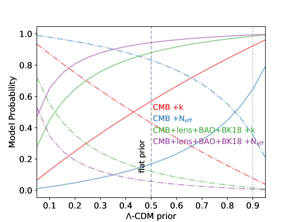
Figure 6: Prior dependence of the model posterior probabilities for the two-models problems considered in this work: the model posterior probability for the comparison $\Lambda$CDM vs K-$\Lambda$CDM for CMB only and the full dataset respectively; the model posterior probabilities relative to the comparison $\Lambda$CDM vs $N_{\rm{eff}}$-$\Lambda$CDM  for CMB only and the full dataset respectively. The solid lines refer to $P(\Lambda\rm{CDM})$, whereas dotted-dashed lines report the K-$\Lambda$CDM and $N_{\rm{eff}}$-$\Lambda$CDM model posterior probabilities ($1-P(\Lambda\rm{CDM})$). The vertical black dashed and dotted lines report the split prior, and a more extreme $90\%:10\%$ allocation in favour of $\Lambda$CDM, respectively.

In this paper we have presented an updated review, following the spirit of previous works [42, 4], addressing current questions in Cosmology through Bayesian Model Averaging. This methodology provided us with a principled approach to assign posterior probabilities to different models, in a Bayesian context, and to seamlessly propagate this additional source of uncertainty all the way to the estimated cosmological parameters. In other words, we let the data express a preference—or lack thereof—between different models. The analysis has been carried out exploiting the importance sampling approach presented in [4] (Fast-MPC).

Firstly, we addressed the curvature problem, by considering the flat $\Lambda$CDM model and the curved K-$\Lambda$CDM. We found that the CMB data alone is not sufficient to express a strong preference for one either the models; when CMB lensing, BAO and the BK 2018 data are included a strong preference for the flat $\Lambda$CDM is found corresponding to a model posterior probability larger than 80%.

We then considered three models for the evolution of Dark Energy: the standard $\Lambda$CDM with a cosmological constant $\Omega_{\Lambda}\approx 0.7$, a DE component with a constant EOS $w=w_{0}$ and a DE component with a time-varying EOS $w=w_{0}+(1-a)w_{\rm a}$. We found that the combination of CMB, lensing, BAO and BK 2018 data, under a flat model prior, only express a mild preference for the standard $\Lambda$CDM with a $\sim$60% probability, against a $\sim$40% probability associated to the $w_{\rm{0}}$CDM. The more complex $w_{\rm{0}}$$w_{\rm{a}}$CDM is highly disfavoured with $\lesssim 1\%$ probability.

For the inflationary scalar spectral index, we considered three models here: the standard $\Lambda$CDM model with varying $n_{\rm{s}}$, a Harrison-Zeldovich spectrum, corresponding to a fixed $n_{\rm s}=1$ and an extended model with varying $n_{\rm{s}}$ and running of the spectral index $n_{\rm{run}}$. We considered the CMB data alone for this problem, and found a very high preference for the most complex $n_{\rm{run}}$-$\Lambda$CDM model, with a probability of  93% when a flat model prior is assumed.

Finally, we investigated the possibility of having additional massless hot-dark matter species in the Universe by varying the $N_{\rm{eff}}$ parameter. We found that the CMB alone expresses a strong preference for the more complex model, $N_{\rm{eff}}$-$\Lambda$CDM  with a high probability of  83% under a flat model prior; conversely, the wider dataset that includes CMB, lensing, BAO and BK 2018 favours the standard $\Lambda$CDM model, with a probability of  94% (with a flat model prior). This tension between data is interesting, and hints at unknown systematics in a similar direction to that of changing $N_{\rm{eff}}$. Further investigation is warranted in this direction.

We have tested the impact of different model prior choices in the two-model applications, namely the curvature and the $N_{\rm{eff}}$-$\Lambda$CDM extensions. We show in Fig. 6 the model posterior probability dependence from the initial model prior choice (solid: $\Lambda$CDM, dot-dashed: K-$\Lambda$CDM, $N_{\rm{eff}}$-$\Lambda$CDM), when considering different datasets. While the priors are obviously important for our inferences, we see that our conclusions for these models are relatively robust to a range of prior probabilities around the flat value.

We also assessed the impact of our model uncertainty marginalization through BMA on the Hubble tension, and found, consistent with current literature, that the model uncertainty does not solve the discrepancy in the Hubble parameter estimate from CMB and BAO versus SNIa. However, we highlight the role BMA could play in discriminating between models in terms of the preference expressed by data themselves.

In conclusion, our work has used BMA and the method of [4] to address four interesting model choices within cosmology. Considering decisions between 2 or 3 models, we have let the data tell us whether any extensions to $\Lambda$CDM are required. The most interesting result from our work is that of the strong preference for running of the spectral index, suggesting that the current data are of sufficient quality that this should be brought into the baseline model. I.e. an extension to assuming a 7-parameter baseline for future analyses should be considered, particularly with the release of results from stage-IV Dark Energy experiments including the Dark Energy Spectroscopic Instrument (DESI; [43]) and the Euclid satellite mission [44, 45].

References

- [1] C.L. Bennett, D. Larson, J.L. Weiland, N. Jarosik, G. Hinshaw, N. Odegard et al., Nine-year wilkinson microwave anisotropy probe (wmap) observations: Final maps and results, The Astrophysical Journal Supplement Series 208 (2013) 20.
- [2] Planck Collaboration, Aghanim, N., Akrami, Y., Ashdown, M., Aumont, J., Baccigalupi, C. et al., Planck 2018 results - vi. cosmological parameters, A&A 641 (2020) A6.
- [3] J.A. Hoeting, D. Madigan, A.E. Raftery and C.T. Volinsky, Bayesian model averaging: A tutorial, Statistical Science 14 (1999) 382.
- [4] S. Paradiso, M. DiMarco, M. Chen, G. McGee and W.J. Percival, A convenient approach to characterizing model uncertainty with application to early dark energy solutions of the Hubble tension, Monthly Notices of the Royal Astronomical Society 528 (2024) 1531 [https://academic.oup.com/mnras/article-pdf/528/2/1531/56410678/stae101.pdf].
- [5] J.A. Frieman, M.S. Turner and D. Huterer, Dark energy and the accelerating universe, Annual Review of Astronomy and Astrophysics 46 (2008) 385 [https://doi.org/10.1146/annurev.astro.46.060407.145243].
- [6] A.R. Liddle, How many cosmological parameters, Monthly Notices of the Royal Astronomical Society 351 (2004) L49 [https://academic.oup.com/mnras/article-pdf/351/3/L49/3604253/351-3-L49.pdf].
- [7] R. Trotta, Bayes in the sky: Bayesian inference and model selection in cosmology, Contemporary Physics 49 (2008) 71 [https://doi.org/10.1080/00107510802066753].
- [8] S. Alam, M. Aubert, S. Avila, C. Balland, J.E. Bautista, M.A. Bershady et al., Completed SDSS-IV extended Baryon Oscillation Spectroscopic Survey: Cosmological implications from two decades of spectroscopic surveys at the Apache Point Observatory, Physical Review D 103 (2021) 083533 [2007.08991].
- [9] A.G. Riess, S. Casertano, W. Yuan, L.M. Macri and D. Scolnic, Large Magellanic Cloud Cepheid Standards Provide a 1% Foundation for the Determination of the Hubble Constant and Stronger Evidence for Physics Beyond LambdaCDM, Astrophys. J. 876 (2019) 85 [1903.07603].
- [10] E. Di Valentino, A. Melchiorri and J. Silk, Reconciling planck with the local value of h0 in extended parameter space, Physics Letters B 761 (2016) 242.
- [11] J.C. Hill, E. McDonough, M.W. Toomey and S. Alexander, Early dark energy does not restore cosmological concordance, Phys. Rev. D 102 (2020) 043507.
- [12] M. Archidiacono, S. Gariazzo, C. Giunti, S. Hannestad and T. Tram, Sterile neutrino self-interactions: H0 tension and short-baseline anomalies, Journal of Cosmology and Astroparticle Physics 2020 (2020) 029.
- [13] M.G. Dainotti, B. De Simone, T. Schiavone, G. Montani, E. Rinaldi and G. Lambiase, On the Hubble Constant Tension in the SNe Ia Pantheon Sample, The Astrophysical Journal 912 (2021) 150 [2103.02117].
- [14] E.D. Valentino, O. Mena, S. Pan, L. Visinelli, W. Yang, A. Melchiorri et al., In the realm of the hubble tension—a review of solutions*, Classical and Quantum Gravity 38 (2021) 153001.
- [15] H. Akaike, A new look at the statistical model identification, IEEE Transactions on Automatic Control 19 (1974) 716.
- [16] M.Y.J. Tan and R. Biswas, The reliability of the Akaike information criterion method in cosmological model selection, Monthly Notices of the Royal Astronomical Society 419 (2012) 3292 [https://academic.oup.com/mnras/article-pdf/419/4/3292/9506848/mnras0419-3292.pdf].
- [17] M. Stone, Cross-validatory choice and assessment of statistical predictions, Journal of the Royal Statistical Society: Series B (Methodological) 36 (1974) 111 [https://rss.onlinelibrary.wiley.com/doi/pdf/10.1111/j.2517-6161.1974.tb00994.x].
- [18] M.A. Newton and A.E. Raftery, Approximate bayesian inference with the weighted likelihood bootstrap, Journal of the Royal Statistical Society. Series B (Methodological) 56 (1994) 3.
- [19] D.I. Hastie and P.J. Green, Model choice using reversible jump markov chain monte carlo, Statistica Neerlandica 66 (2012) 309 [https://onlinelibrary.wiley.com/doi/pdf/10.1111/j.1467-9574.2012.00516.x].
- [20] Tristram, M., Banday, A. J., Douspis, M., Garrido, X., Górski, K. M., Henrot-Versillé, S. et al., Cosmological parameters derived from the final planck data release (pr4), A&A 682 (2024) A37.
- [21] Planck Collaboration, Aghanim, N., Akrami, Y., Ashdown, M., Aumont, J., Baccigalupi, C. et al., Planck 2018 results - v. cmb power spectra and likelihoods, A&A 641 (2020) A5.
- [22] Planck collaboration, Planck 2018 results. VIII. Gravitational lensing, Astron. Astrophys. 641 (2020) A8 [1807.06210].
- [23] A.J. Ross, L. Samushia, C. Howlett, W.J. Percival, A. Burden and M. Manera, The clustering of the SDSS DR7 main Galaxy sample – I. A 4 per cent distance measure at , Mon. Not. Roy. Astron. Soc. 449 (2015) 835 [1409.3242].
- [24] P. Carter, F. Beutler, W.J. Percival, C. Blake, J. Koda and A.J. Ross, Low redshift baryon acoustic oscillation measurement from the reconstructed 6-degree field galaxy survey, Monthly Notices of the Royal Astronomical Society 481 (2018) 2371 [https://academic.oup.com/mnras/article-pdf/481/2/2371/25791913/sty2405.pdf].
- [25] BOSS collaboration, The clustering of galaxies in the completed SDSS-III Baryon Oscillation Spectroscopic Survey: cosmological analysis of the DR12 galaxy sample, Mon. Not. Roy. Astron. Soc. 470 (2017) 2617 [1607.03155].
- [26] S. Alam, M. Aubert, S. Avila, C. Balland, J.E. Bautista, M.A. Bershady et al., Completed sdss-iv extended baryon oscillation spectroscopic survey: Cosmological implications from two decades of spectroscopic surveys at the apache point observatory, Phys. Rev. D 103 (2021) 083533.
- [27] BICEP/Keck Collaboration collaboration, Improved constraints on primordial gravitational waves using planck, wmap, and bicep/keck observations through the 2018 observing season, Phys. Rev. Lett. 127 (2021) 151301.
- [28] J. Torrado and A. Lewis, Cobaya: Code for Bayesian Analysis of hierarchical physical models, JCAP 05 (2021) 057 [2005.05290].
- [29] J. Torrado and A. Lewis, “Cobaya: Bayesian analysis in cosmology.” Astrophysics Source Code Library, record ascl:1910.019, Oct., 2019.
- [30] A. Lewis, GetDist: a Python package for analysing Monte Carlo samples, 1910.13970.
- [31] Planck Collaboration, P.A.R. Ade, N. Aghanim, M. Arnaud, M. Ashdown, J. Aumont et al., Planck 2015 results. XIII. Cosmological parameters, A&A 594 (2016) A13 [1502.01589].
- [32] E. Rosenberg, S. Gratton and G. Efstathiou, CMB power spectra and cosmological parameters from Planck PR4 with CamSpec, Monthly Notices of the Royal Astronomical Society 517 (2022) 4620 [2205.10869].
- [33] A.G. Riess, A.V. Filippenko, P. Challis, A. Clocchiatti, A. Diercks, P.M. Garnavich et al., Observational evidence from supernovae for an accelerating universe and a cosmological constant, The Astronomical Journal 116 (1998) 1009.
- [34] S. Perlmutter, G. Aldering, G. Goldhaber, R.A. Knop, P. Nugent, P.G. Castro et al., Measurements of and from 42 high-redshift supernovae, The Astrophysical Journal 517 (1999) 565.
- [35] A.H. Guth, Inflationary universe: A possible solution to the horizon and flatness problems, Phys. Rev. D 23 (1981) 347.
- [36] P.J. Steinhardt and M.S. Turner, A Prescription for Successful New Inflation, Phys. Rev. D 29 (1984) 2162.
- [37] N.Y. Gnedin and O.Y. Gnedin, Cosmological neutrino background revisited, The Astrophysical Journal 509 (1998) 11.
- [38] G. Mangano, G. Miele, S. Pastor, T. Pinto, O. Pisanti and P.D. Serpico, Relic neutrino decoupling including flavour oscillations, Nuclear Physics B 729 (2005) 221.
- [39] P.F. de Salas and S. Pastor, Relic neutrino decoupling with flavour oscillations revisited, Journal of Cosmology and Astroparticle Physics 2016 (2016) 051.
- [40] E. Di Valentino, S. Gariazzo, W. Giarè and O. Mena, Impact of the damping tail on neutrino mass constraints, Phys. Rev. D 108 (2023) 083509.
- [41] E. Di Valentino, S. Gariazzo and O. Mena, Model marginalized constraints on neutrino properties from cosmology, Phys. Rev. D 106 (2022) 043540.
- [42] D. Parkinson and A.R. Liddle, Bayesian model averaging in astrophysics: a review, Statistical Analysis and Data Mining: The ASA Data Science Journal 6 (2013) 3 [https://onlinelibrary.wiley.com/doi/pdf/10.1002/sam.11179].
- [43] DESI Collaboration, A. Aghamousa, J. Aguilar, S. Ahlen, S. Alam, L.E. Allen et al., The DESI Experiment Part I: Science,Targeting, and Survey Design, arXiv e-prints (2016) arXiv:1611.00036 [1611.00036].
- [44] R. Laureijs, J. Amiaux, S. Arduini, J.L. Auguères, J. Brinchmann, R. Cole et al., “Euclid definition study report.” oct, 2011.
- [45] Euclid Collaboration, R. Scaramella, J. Amiaux, Y. Mellier, C. Burigana, C.S. Carvalho et al., Euclid preparation. I. The Euclid Wide Survey, A&A 662 (2022) A112 [2108.01201].