Microscopic Theory of Cooper-pair fluctuations in a 2D Electron System with Strong Spin-Orbit Scatterings: Phase Separation and Large Magnetoresistance

Abstract

A microscopic theory of Cooper-pair fluctuations (CPFs) in a 2D electron system with strong spin-orbit scatterings is presented to account for the observation, at low temperatures, of large magnetoresistance (MR) above a crossover field to superconductivity in electron-doped SrTiO₃/LaAlO₃ interfaces. It is found that, while the conventional (diagrammatic) microscopic theory of superconducting fluctuations fails to account for the pronounced MR, an extension of the theory, which introduces a proper definition of the CPFs density, reveals an operative mechanism of this intriguing effect. Phase separation due to Coulomb repulsion, from the rarefying unpaired normal-state electron gas, following field-induced condensation of CPFs in real-space mesoscopic puddles, are in the core of this mechanism. These findings enable us to amend the state-of-the-art microscopic theory, in a consistent manner with the time dependent GL functional approach used previously in an extensive account of the experimentally reported effect.

I Introduction

It was shown recently MZPRB2021 ,MZJPC2023 that Cooper-pair fluctuations (CPFs) in a 2D electron system with strong spin-orbit scatterings can lead at low temperatures to pronounced magnetoresistance (MR) above a crossover field to superconductivity. Employing the time dependent Ginzburg-Landau (TDGL) functional approach the model was applied to the high mobility electron systems formed in the electron-doped interfaces between two insulating perovskite oxides—SrTiO₃ and LaAlO₃ Ohtomo04 ,Caviglia08 , showing good quantitative agreement with a large body of experimental sheet-resistance data obtained under varying gate voltage Mograbi19 (see also RoutPRL2017 ,ManivNatCommun2015 ).

In the present paper we approach the same problem from the point of view of the conventional (diagrammatic) microscopic theory of fluctuations in superconductors, developed by Larkin and Varlamov (LV) LV05 . We have found that, while the state-of-the-art microscopic theory of superconducting fluctuations at very low temperatures GalitLarkinPRB01 , Glatzetal2011 , Lopatinetal05 , Khodas2012 fails to account for the pronounced MR, a proper definition of the density of CPFs enables us to show that under increasing field and diminishing temperature CPFs condense in real space mesoscopic puddles, and then phase separate due to Coulomb repulsion from their source (unpaired) normal-state electrons to achieve interphase dynamical equilibrium. It has been, therefore, concluded that during the extended life-time of CPFs in their mesoscopic enclaves, when the fluctuation paraconductivity diminishes, the density of the normal-state conduction electrons is also suppressed (due to charge transfer to the localized CPFs) and so yielding overall large MR. The crossover to this state of pronounced MR is, therefore, associated with the instability of the nearly uniform system of CPFs to formation, under increasing field at low temperature, of highly inhomogeneous system of CPFs puddles. These results enable us to amend the LV microscopic theory, in a consistent manner with the TDGL functional approach presented in Refs.MZPRB2021 , MZJPC2023 .

The paper is organized as follows: In Sec.II we present the model of a 2D electron system with strong spin-orbit scatterings employed in this paper. The model is then applied in Sec.III to the microscopic (zero field) LV theory at very low temperature. Subsequently, in the same section, the results of the microscopic (diagrammatic) theory for the fluctuation conductivity are compared to those of the corresponding TDGL functional approach, revealing important connections between the two approaches. In Sec.IV we present an extension of the microscopic theory of fluctuation conductivity to finite magnetic field, which is further developed in Sec.V by introducing the concept of CPFs density. The phenomenon of field-induced condensation of CPFs at very low temperatures, revealed in analyzing this concept, and its consequent phenomenon of crossover to localization and phase separation of CPFs, are also discussed in Sec.V.  A detailed discussion of the physical ramifications of the main findings of this paper and concluding remarks appear in SecVI.

II The model

The model employed in this paper, following Refs. MZPRB2021 ,MZJPC2023 , which have been motivated by the perovskite oxides electronic interface state investigated in Ref. Mograbi19 , consists of a thin rectangular film of electrons, subject to strong spin-orbit impurity scattering Abrikosov62 , Klemm75 , under a strong magnetic field $H$, applied parallel to the conducting plane. We assume, for simplicity of the analysis, that spin-orbit interaction dominates the impurity scatterings. Superconductivity in this system is governed both by the Zeeman spin splitting energy,$\mu_{B}H$ and the spin-orbit scattering rate, $1/\tau_{SO}\equiv\varepsilon_{SO}/\hbar$ (see a detailed description in early papers dealing with similar 3D systems Maki66 , FuldeMaki70 , WHH66 ).

We use a reference of frame in which the conducting interface is in its $z-x$ plane, the film thickness (along the $y$ axis) is $d$, and $\mathbf{E}\mathbf{\mathbf{=}}\widehat{x}E$,  $\mathbf{B}\mathbf{=}\widehat{z}H$ are the in-plane electric and magnetic fields, respectively. The transport calculations are carried out in the linear response approximation with respect to the electric field and impurity scattering is treated in the dirty limit, i.e. for $k_{B}T\tau_{SO}/\hbar\ll 1$ (see also, below, an extension of the dirty limit condition in the presence of magnetic field). Typical values of the parameters of the electronic system used are: $E_{F}\simeq 7m\boldsymbol{\mathit{eV}},\varepsilon_{SO}\simeq 3m\boldsymbol{\mathit{eV}},d\simeq 10^{-9}\boldsymbol{\mathit{m}}$, and the characteristic magnetic field of the crossover to superconductivity at zero temperature is $H_{c\parallel 0}=4.5\boldsymbol{\mathit{T}}$. Under these circumstances the Zeeman spin-splitting energy: $\mu_{B}H_{c\parallel 0}\simeq 0.26m\boldsymbol{\mathit{eV}}$, is much larger than the diamagnetic (kinetic) energy: $\hslash D\left(deH_{c\parallel 0}/\hbar\right)^{2}\simeq 8\times 10^{-3}m\boldsymbol{\mathit{eV}}$, where $D\equiv\tau_{SO}v_{F}^{2}/2=\hbar E_{F}/\varepsilon_{SO}m^{\ast}$ is the electronic diffusion coefficient, with the electronic band effective mass $m^{\ast}$ close to the free electron mass $m_{e}$. We, therefore neglect the diamagnetic energy in our analysis below.

Our model is similar to the models employed in both Refs.Lopatinetal05 and Khodas2012 , but differs in two important aspects. In our model impurity scatterings are dominated by spin-orbit interactions whereas in Refs.Lopatinetal05 , Khodas2012 spin-orbit interaction was absent. Also, in our model we incorporate self-consistent interactions between fluctuations, which remove the quantum critical point, whereas in both Refs.Lopatinetal05 and Khodas2012 quantum criticality played a major role.

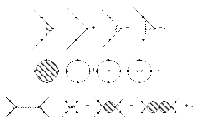
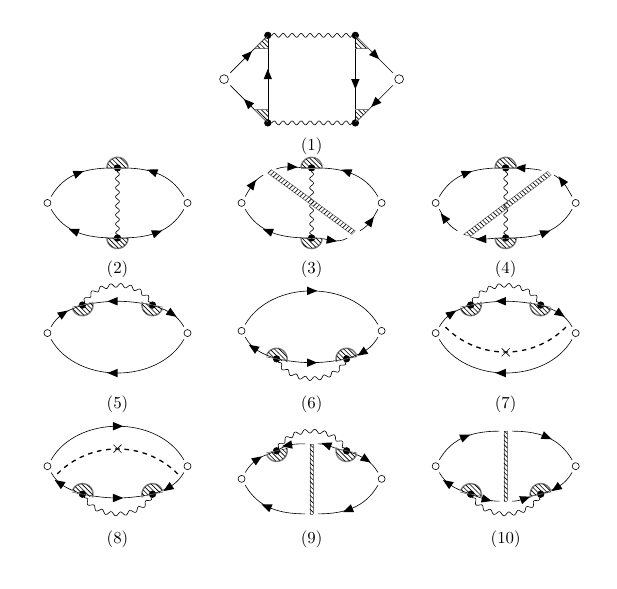
Figure 1: Right figure:  Leading-order Feynman diagrams of the current-current correlator contributing to the fluctuation conductivity. Small empty circles are bare current vertices, solid lines are impurity average normal-state Green’s functions, wavy lines are fluctuation propagators, small full circles are bare pairing vertices, dashed areas stand for impurity ladders between two electron lines, dashed lines with central crosses are additional impurity renormalizations. Left figure: External (upper row) and internal (middle row) impurity-scattering renormalization of pairing vertices appearing in the Feynman diagrams on the right and in the fluctuation propagator (lower row on the left).

III TDGL functional approach vs. microscopic theory at zero field

III.1 The microscopic Larkin-Varlamov (diagrammatic) theory

In this subsection we introduce the formalism, employed by LV for the zero magnetic field situation at temperatures above the zero-field transition temperature $T_{c0}$, in a general form which allows extension to finite field at low temperatures well below $T_{c0}$. It is implicitly assumed, throughout this paper, that the critical shift parameter $\varepsilon$ (or $\varepsilon_{H}$ for the finite-field situations, see below for more details) includes high-order terms in the Gorkov GL expansion, self-consistently in the interaction between fluctuations UllDor90 ,UllDor91 , as done in Ref.MZPRB2021 .

As indicated in Sec.II, the incorporation of such interactions self-consistently into the equation determining the ”critical” shift parameter avoids it vanishing at any field and temperature and so, in particular, removes the quantum critical point (Lopatinetal05 , Khodas2012 ). Our motivation in selecting this approach is the absence of genuine zero resistance in the experimental data reported in Ref.Mograbi19 , even at zero field.

III.1.1 The Aslamazov-Larkin paraconductivity diagram

The principal contribution to the conductivity due to CPFs (paraconductivity) in the microscopic (diagrammatic) theory is associated with the Aslamazov-Larkin (AL) diagram AL68 (Number 1 in Fig.1, see also Fig.2). The corresponding time-ordered current-current correlator in (Matsubara) imaginary frequency representation is written as:

$$Q_{xx}^{LV(1)}\left(i\Omega_{\nu}\right)=-4e^{2}k_{B}T\sum\limits_{k=-\infty}^{\infty}\frac{1}{d}\left(\frac{1}{2\pi}\right)^{2}\int d^{2}q$$ (1)

$$\times\mathcal{D}\left(q,\Omega_{k}+\Omega_{\nu}\right)B_{x}\left(q,\Omega_{k},\Omega_{\nu}\right)\mathcal{D}\left(q,\Omega_{k}\right)B_{x}\left(q,\Omega_{k},\Omega_{\nu}\right)$$

where:

$$\mathcal{D}\left(q,\Omega_{k}\right)=\frac{1}{N_{2D}\left[\varepsilon+\frac{\pi\hbar}{8k_{B}k_{B}T}\left(Dq^{2}+\Omega_{k}\right)\right]}$$

is the fluctuation propagator in wavenumber-(Matsubara) frequency representation, $\varepsilon=\ln\left(T/T_{c0}\right)$, $T_{c0}$ is the zero-field transition temperature, $D=\tau_{SO}v_{F}^{2}/2$ is the electronic diffusion coefficient, and $v_{F}=\hbar k_{F}/m^{\ast}$ is the Fermi velocity. Here $\Omega_{k}=2kk_{B}T/\hbar,\Omega_{\nu}=2\nu k_{B}T/\hbar,$ $k=0,\pm 1,\pm 2,...,$       $\nu=0,1,2,....$ are bosonic Matsubara frequencies and $N_{2D}=m^{\ast}/2\pi\hbar^{2}$ is the single-electron density of states (DOS), with an effective mass $m^{\ast}$.

In Eq.1 the effective current vertex part (see Fig.2) is given by:

$$B_{x}\left(q,\Omega_{k},\Omega_{\nu}\right) = k_{B}T\sum\limits_{n=-\infty}^{\infty}\lambda\left(q,\omega_{n}+\Omega_{\nu},\Omega_{k}-\omega_{n}\right)\lambda\left(q,\omega_{n},\Omega_{k}-\omega_{n}\right)\times$$

$$\left(\frac{1}{2\pi}\right)^{2}\int d^{2}pG\left(\mathbf{p},\omega_{n}+\Omega_{\nu}\right)G\left(\mathbf{p},\omega_{n}\right)G\left(\mathbf{q-p},\Omega_{k}-\omega_{n}\right)v_{x}\left(\mathbf{p}\right)$$

where $\omega_{n}=\left(2n+1\right)k_{B}T/\hbar,n=0,\pm 1,\pm 2,...$ , is a fermionic Matsubara frequency, and $\lambda$ stands for a three-leg vertex of two electron lines and a fluctuation line, renormalized by impurity-scattering ladder (see left Fig.1). A single-electron line corresponds to the Green’s function: $G\left(\mathbf{p},\omega_{n}\right)=1/\left[i\hbar\widetilde{\omega}_{n}-\hbar^{2}\left(p^{2}-k_{F}^{2}\right)/2m^{\ast}\right]$, whereas the ”bare” current vertex is: $v_{x}\left(\mathbf{p}\right)=\hbar p_{x}/m^{\ast}$.

At zero magnetic field, following LV, we have:

$$\lambda\left(q,\omega_{n},\Omega_{k}-\omega_{n}\right)=\frac{\left|\widetilde{\omega}_{n}-\left(\widetilde{\Omega_{k}-\omega}_{n}\right)\right|}{\left|2\omega_{n}-\Omega_{k}\right|+\frac{v_{F}^{2}q^{2}}{2\tau_{SO}\left|\widetilde{\omega}_{n}-\left(\widetilde{\Omega_{k}-\omega}_{n}\right)\right|^{2}}}$$ (3)

where $\widetilde{\omega}_{n}=\omega_{n}+\left(1/2\tau_{SO}\right)sign\left(\omega_{n}\right)$, whereas $B_{x}\left(q,\Omega_{k};\Omega_{\nu}\right)$ is approximated by taking: $\Omega_{\nu}=0,$ $\Omega_{k}=0$, so that:

$$B_{x}\left(q,\Omega_{k},\Omega_{\nu}\right)\simeq B_{x}\left(q,0,0\right)=k_{B}T\sum\limits_{n=-\infty}^{\infty}\lambda^{2}\left(q,\omega_{n},-\omega_{n}\right)$$

$$\left(\frac{1}{2\pi}\right)^{2}\int d^{2}pG\left(\mathbf{p},\omega_{n}\right)G\left(\mathbf{p},\omega_{n}\right)G\left(\mathbf{q-p},-\omega_{n}\right)v_{x}\left(\mathbf{p}\right)$$

and:

$$\lambda\left(q,\omega_{n},-\omega_{n}\right)=\frac{\left|\widetilde{\omega}_{n}\right|}{\left|\omega_{n}\right|+\frac{v_{F}^{2}q^{2}}{4\tau_{SO}\left|2\widetilde{\omega}_{n}\right|^{2}}}\simeq\frac{\left|\widetilde{\omega}_{n}\right|}{\left|\omega_{n}\right|+\frac{1}{2}Dq^{2}}$$ (4)

Performing the integration over the electronic wavevector and the Matsubara frequency summation we find:

$$B_{x}\left(q,0,0\right)\approx-N_{2D}\tau_{SO}v_{F}^{2}q_{x}\frac{1}{4\pi k_{B}T}\psi^{\prime}\left(\frac{1}{2}+\frac{D}{4\pi k_{B}T}q^{2}\right)$$ (5)

where $\psi$ is digamma function.

Neglecting the $q$ dependence, i.e. taking $B_{x}\left(q\rightarrow 0,0,0\right)\rightarrow-2N_{2D}\eta_{\left(2\right)}q_{x}$, with:

$$\eta_{\left(2\right)}=\frac{\pi\hbar D}{8k_{B}T}$$ (6)

the corresponding expression for the zero-field AL conductivity is found to be identical to the LV integral form of the well-known result:

$$\sigma_{AL}^{LV}=\frac{e^{2}}{8\hbar d}\int d\left(\eta_{\left(2\right)}q^{2}\right)\frac{\left(\eta_{\left(2\right)}q^{2}\right)}{\left(\varepsilon+\eta_{\left(2\right)}q^{2}\right)^{3}}$$

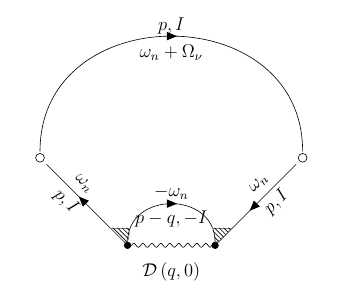
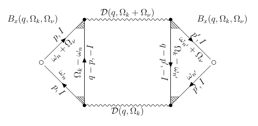
Figure 2: Lower figure: AL diagram consisting of effective current vertices ($B_{x}$) and fluctuation propagators ($\mathcal{D}$). Upper figure: DOS conductivity diagram illustrating the mechanism in which electron time of coherence is suppressed due to electron scattering by background electrons via virtual exchange of CPF with $q\neq 0$ and $I\neq 0$.

III.1.2 The DOS conductivity diagrams

The next leading contributions to the fluctuation conductivity in the LV scheme corresponds to four bubble-shaped diagrams (numbers 5-8 in Fig.1), termed density-of-states diagrams, due to the fluctuation self-energy insertion to single-electron lines. Other, topologically distinct diagrams of the same order in the fluctuations propagators, (see in Fig.1 the diagrams numbered 2-4) can be shown to be negligible (see Appendix A and Refs.ManivAlexanderJPC1976 ,MakiPTP1968 ,ThompsonPRB1970 ,ManivAlexanderJPC1977 ). Furthermore, as explained in LV, the DOS diagrams 9,10 can also be neglected, however at very low temperature and close to the quantum critical point they dominate the conductivity (see Refs.Lopatinetal05 , Glatzetal2011 , Khodas2012 ). We will return to the issue of quantum critical fluctuations in Sec.VI.

The current-current correlator corresponding, e.g. to diagram 5 (see also Fig.2 upper part) is written as:

$$Q_{xx}^{LV(5)}\left(i\Omega_{\nu}\right)=-2e^{2}k_{B}T\sum\limits_{k=-\infty}^{\infty}\frac{1}{d}\left(\frac{1}{2\pi}\right)^{2}$$

$$\times\int d^{2}q\Sigma_{xx}^{(5)}\left(q,\Omega_{k},\Omega_{\nu}\right)\mathcal{D}\left(q,\Omega_{k}\right)$$ (7)

where:

$$\Sigma_{xx}^{(5)}\left(q,\Omega_{k},\Omega_{\nu}\right)=k_{B}T\sum\limits_{n=-\infty}^{\infty}\lambda^{2}\left(q,\omega_{n},\Omega_{k}-\omega_{n}\right)$$

$$\times I_{xx}^{(5)}\left(\mathbf{q},\omega_{n},\Omega_{k},\Omega_{\nu}\right)$$ (8)

and:

$$I_{xx}^{(5)}\left(\mathbf{q},\omega_{n},\Omega_{k},\Omega_{\nu}\right)=\left(\frac{1}{2\pi}\right)^{2}\int d^{2}pG^{2}\left(\mathbf{p},\omega_{n}\right)$$

$$G\left(\mathbf{q-p},\Omega_{k}-\omega_{n}\right)G\left(\mathbf{p},\omega_{n}+\Omega_{\nu}\right)v_{x}^{2}\left(\mathbf{p}\right)$$ (9)

Neglecting dynamical (quantum critical) fluctuations by restricting consideration only to the single term with $\Omega_{k}=0$ in the summation over $k$ in Eq.7, performing the integration over the electron wavevector in Eq.9 and the Matsubara frequency summation in Eq.8, we get after the analytic continuation: $\Omega_{\nu}\rightarrow-i\omega$:

$$\Sigma_{xx}^{(5)}\left(q,\Omega_{k}=0,\Omega_{\nu}\rightarrow-i\omega\right)\approx-\frac{i\omega\tau_{SO}^{2}v_{F}^{2}N_{2D}}{8\pi k_{B}T\hbar}\times$$

$$\left[\psi^{\prime}\left(\frac{1}{2}+\frac{\hbar}{4\pi k_{B}T\tau_{SO}}\right)-\frac{3\hbar}{4\pi k_{B}T\tau_{SO}}\psi^{\prime\prime}\left(\frac{1}{2}+\frac{\hbar Dq^{2}}{4\pi k_{B}T}\right)\right]$$

$$\approx\frac{i\omega DN_{2D}}{4\pi k_{B}T}\frac{3}{4\pi k_{B}T}\psi^{\prime\prime}\left(\frac{1}{2}+\frac{\hbar Dq^{2}}{4\pi k_{B}T}\right)$$ (10)

Further simplification, consistent with the procedure used in evaluating the AL contribution, is achieved by neglecting the $q$ dependence of $\Sigma_{xx}^{(5)}\left(q,\Omega_{k}=0,\Omega_{\nu}\rightarrow-i\omega\right)$ in Eq.7, that is:

$$\Sigma_{xx}^{(5)}\left(q\rightarrow 0,\Omega_{k}=0,\Omega_{\nu}\rightarrow-i\omega\right)\rightarrow\frac{i\omega DN_{2D}}{4\pi k_{B}T}\frac{3}{4\pi k_{B}T}\psi^{\prime\prime}\left(\frac{1}{2}\right)$$

which yields for the corresponding contribution to the fluctuation conductivity:

$$\sigma_{xx}^{LV\left(5\right)}=-\lim_{\omega\rightarrow 0}\frac{Q_{xx}^{LV\left(5\right)}\left(\omega\right)}{i\omega}\simeq-\frac{3e^{2}}{4\hbar d}\frac{14\zeta\left(3\right)}{\pi^{4}}\int\frac{d\left(\eta_{\left(2\right)}q^{2}\right)}{\varepsilon+\left(\eta_{\left(2\right)}q^{2}\right)}$$

where we have used the identity: $\psi^{\prime\prime}\left(1/2\right)=-\sum\limits_{n=0}^{\infty}1/\left(n+1/2\right)^{3}=-14\zeta\left(3\right)$.

An identical result is obtained for diagram No.6 (see Fig.1), i.e.: $\sigma_{xx}^{LV\left(6\right)}=\sigma_{xx}^{LV\left(5\right)}$.  A similar method of calculation yields for the 7-th diagram (see also Refs.AltshulerJETP1983 , Dorin-etal-PRB1993 ):

$$\sigma_{xx}^{LV\left(7\right)}\simeq\frac{e^{2}}{4\hbar d}\frac{14\zeta\left(3\right)}{\pi^{4}}\int\frac{d\left(\eta_{\left(2\right)}q^{2}\right)}{\varepsilon+\left(\eta_{\left(2\right)}q^{2}\right)}=-\frac{1}{3}\sigma_{xx}^{LV\left(5\right)}$$

so that together with the identity: $\sigma_{xx}^{LV\left(7\right)}=\sigma_{xx}^{LV\left(8\right)}$ one finds:

$$\sigma_{xx}^{LV\left(5+6+7+8\right)}=2\sigma_{xx}^{LV\left(5+7\right)}=$$

$$-\frac{e^{2}}{\hbar d}\left(\frac{14\zeta\left(3\right)}{\pi^{4}}\right)\int\frac{d\left(\eta_{\left(2\right)}q^{2}\right)}{\varepsilon+\left(\eta_{\left(2\right)}q^{2}\right)}$$ (11)

III.2 Comparison with the TDGL functional approach

III.2.1 The Aslamazov-Larkin paraconductivity

The TDGL functional $\mathfrak{L}\left(\Delta,\mathbf{A}\right)$ of the order parameter $\Delta\left(\boldsymbol{r},t\right)$ and vector potential $\mathbf{A}\left(\boldsymbol{r},t\right)$ determines the Cooper-pairs current density FuldeMaki70 :

$$\mathbf{j}\left(\mathbf{r},t\right)=-c\frac{\partial\mathfrak{L}\left(\Delta\left(\mathbf{r},t\right),\mathbf{A}\left(\mathbf{r},t\right)\right)}{\partial\mathbf{A}\left(\mathbf{r},t\right)}$$ (12)

responsible for the AL paraconductivity (see Appendix B).

In this approach the entire underlying information about the thin film of pairing electrons system is incorporated in the inverse fluctuation propagator (in wavevector-frequency representation) $D^{-1}\left(\mathbf{q+}2e\mathbf{A/\hbar},\omega\right)$, mediating between the order parameter and the GL functional. In the Gaussian approximation the relation is quadratic, i.e.:

$$\mathfrak{L}\left(\Delta,\mathbf{A}\right) = \frac{1}{d}\int\frac{d^{2}q}{\left(2\pi\right)^{2}}\left(\frac{1}{2\pi}\right)\int d\Omega\left|\Delta\left(\mathbf{q},\Omega\right)\right|^{2}\times$$ (13)

$$\mathcal{D}^{-1}\left(\mathbf{q+}2e\mathbf{A/\hbar},\Omega\right)$$

so that the coupling to the external electromagnetic field takes place directly through the vertex of the Cooper-pair current, defined in Eq.(12).

The corresponding AL time-ordered current-current correlator is given by:

$$Q_{AL}\left(i\Omega_{\nu}\right)=\left(4eN_{2D}D\right)^{2}d^{-1}\left(\frac{1}{2\pi}\right)^{2}\int d^{2}qq_{x}^{2}k_{B}T$$ (14)

$$\sum\limits_{k=-\infty}^{\infty}C\left(q,\Omega_{k}+\Omega_{\nu}\right)\mathcal{D}\left(q,\Omega_{k}+\Omega_{\nu}\right)C\left(q,\Omega_{k}\right)\mathcal{D}\left(q,\Omega_{k}\right)$$

where $\Omega_{k}=2kk_{B}T/\hbar,\Omega_{\nu}=2\nu k_{B}T/\hbar,$ $k=0,\pm 1,\pm 2,...,$       $\nu=0,1,2,....$ are bosonic Matsubara frequencies. Here, like in Sec.IIIA1, the electrical current is generated along the $x$ axis, $q_{z},q_{x}$ are the fluctuation (in-plane) wave-vector components along the magnetic and electric field directions, respectively, and $q^{2}\equiv q_{z}^{2}+q_{x}^{2}$.

The fluctuation propagator $\mathcal{D}\left(q,\Omega_{k}\right)$ and its corresponding effective current vertex $C\left(q,\Omega_{k}\right)$ are given by MZPRB2021 :

$$\mathcal{D}\left(q,\Omega_{k}\right) = \frac{1}{N_{2D}\Phi\left(x+\left|k\right|\right)},$$

$$C\left(q,\Omega_{k}\right) = \frac{\Phi^{\prime}\left(x+\left|k\right|\right)}{4\pi k_{B}T}$$ (15)

where for zero field:

$$\Phi\left(x+\left|k\right|\right)=\varepsilon+\psi\left(1/2+x+\left|k\right|\right)-\psi\left(1/2\right)$$ (16)

and: $x=\hbar Dq^{2}/4\pi k_{B}T$.

We now define a normalized effective current vertex analogous to $B_{x}\left(q,0,0\right)$:

$$C_{x}\left(q,\Omega_{k}\right) \equiv 2N_{2D}Dq_{x}C\left(q,\Omega_{k}\right)=2N_{2D}D\frac{\Phi^{\prime}\left(x+\left|k\right|\right)}{4\pi k_{B}T}q_{x}$$ (17)

$$= 2N_{2D}D\frac{\psi^{\prime}\left(\frac{1}{2}+\frac{\hbar\left|\Omega_{k}\right|}{2\pi k_{B}T}+\frac{\hbar Dq^{2}}{4\pi k_{B}T}\right)}{4\pi k_{B}T}q_{x}$$

with the help of which Eq.14 is rewritten in a form similar to Eq.1, i.e.:

$$Q_{AL}\left(i\Omega_{\nu}\right)\simeq 4e^{2}k_{B}T\sum\limits_{k=-\infty}^{\infty}\frac{1}{d}\left(\frac{1}{2\pi}\right)^{2}\times$$ (18)

$$\int d^{2}q\mathcal{D}\left(q,\Omega_{k}+\Omega_{\nu}\right)C_{x}\left(q,\Omega_{k}\right)\mathcal{D}\left(q,\Omega_{k}\right)C_{x}\left(q,\Omega_{k}\right)$$

Taking the static limit, $\Omega_{k}\rightarrow 0$ Eq.17 reduces to:

$$C_{x}\left(q,\Omega_{k}\rightarrow 0\right) \rightarrow 2N_{2D}D\frac{\psi^{\prime}\left(\frac{1}{2}+\frac{\hbar Dq^{2}}{4\pi k_{B}T}\right)}{4\pi k_{B}T}q_{x}$$ (19)

$$= -B_{x}\left(q,0,0\right)$$

The complete agreement between the expressions Eqs.5 and 19, clearly indicates that the effect of the infinite set of ladder diagrams which renormalize the pairing vertices outside the fluctuation propagators (Cooperon insertions) in the AL diagram, within the LV microscopic approach, is fully consistent with the impurity-scatterings effect introduced to the fluctuation current vertex through its relation to the fluctuation propagator within our TDGL functional approach. The corresponding consistency equation between the renormalized current vertex and the fluctuation propagator, inherent to the TDGL functional approach, should also be satisfied within the fully microscopic approach.

Within our TDGL functional approach we note that: $C_{x}\left(q,\Omega_{k}\rightarrow 0\right)=v_{F}^{2}\tau_{SO}\frac{1}{4\pi k_{B}T}N_{2D}\Phi^{\prime}\left(x\right)q_{x}$, whereas: $N_{2D}\Phi^{\prime}\left(x\right)=\left(8\pi k_{B}T/\hbar v_{F}^{2}\tau_{SO}\right)\left[\partial/\partial\left(q^{2}\right)\right]\mathcal{D}^{-1}\left(q,0\right)$, so that:

$$C_{x}\left(q,0\right)=\frac{2q_{x}}{\hbar}\frac{\partial}{\partial\left(q^{2}\right)}\mathcal{D}^{-1}\left(q,0\right)=-B_{x}\left(q,0,0\right)$$ (20)

Equation 20 relates the (Cooperon) external-vertex insertions to the internal-vertex insertions of ladder diagrams introduced in the calculation of the fluctuation propagator. In our TDGL approach it appears naturally, directly from the inverse fluctuation propagator, without taking any additional measure. It reflects the fundamental variation principle, satisfied by the electromagnetically modified GL free energy functional with respect to the vector potential, see Eq.96 in Appendix B.

III.2.2 The DOS conductivity

The basic observable used in evaluating the DOS conductivity within the TDGL approach is the CPFs density:

$$n_{s}=\frac{1}{d}\frac{1}{\left(2\pi\right)^{2}}\int\left\langle\left|\phi\left(q\right)\right|^{2}\right\rangle d^{2}q$$ (21)

with the Cooper-pair momentum distribution function $\left\langle\left|\phi\left(q\right)\right|^{2}\right\rangle$ derived by using the frequency-dependent GL functional, Eq.(13). This is done by rewriting Eq.(13) in terms of the frequency and wavenumber representations GL wavefunctions $\phi\left(q,\Omega\right)$, after analytic continuation to real frequencies $i\Omega_{\mu}\rightarrow\Omega$, i.e.:

$$\mathfrak{L}\left(\Delta\right) = \frac{1}{d}\int\frac{d^{2}q}{\left(2\pi\right)^{2}}\int\frac{d\Omega}{2\pi}\left|\Delta\left(q,\Omega\right)\right|^{2}\mathcal{D}^{-1}\left(q,\Omega\right)$$

$$= \frac{1}{d}\int\frac{d^{2}q}{\left(2\pi\right)^{2}}\int\frac{d\Omega}{2\pi}\left|\phi\left(q,\Omega\right)\right|^{2}L^{-1}\left(q,\Omega\right)=\mathfrak{L}\left(\phi\right)$$

under the normalization relations:

$$\mathcal{D}\left(q,\Omega\right)=\left(\frac{\alpha k_{B}T}{N_{2D}}\right)L\left(q,\Omega\right)$$ (23)

Here the constant $\alpha$ (i.e. independent of $q$ and $\Omega$), determines the normalization of the wavefunctions from the corresponding components of the order parameter through the reciprocal relations (see Appendix C):

$$\left|\phi\left(q,\Omega\right)\right|^{2}=\left(\frac{N_{2D}}{\alpha k_{B}T}\right)\left|\Delta\left(q,\Omega\right)\right|^{2}$$

Following LV, the resulting expression for the momentum distribution function is obtained by exploiting the Langevin force technique in the TDGL equation, which leads to:

$$\left\langle\left|\phi\left(q\right)\right|^{2}\right\rangle=2k_{B}T\gamma_{GL}\int\frac{d\left(\hbar\Omega\right)}{2\pi}\left|L\left(q,\Omega\right)\right|^{2}$$

where:

$$L\left(q,\Omega\right)^{-1}=k_{B}T\alpha\left(\varepsilon+\xi\left(T\right)^{2}q^{2}\right)-i\gamma_{GL}\hbar\Omega$$ (24)

and the CPF coherence length $\xi\left(T\right)$ and dimensionless CPF life-time, $\gamma_{GL}$, are given by:

$$\xi\left(T\right)=\sqrt{\frac{\pi\hbar}{8k_{B}T}D},\gamma_{GL}=\frac{\pi\alpha}{8}=\left(\frac{\pi^{3}}{14\zeta\left(3\right)}\right)\frac{k_{B}T}{E_{F}}$$ (25)

Performing the frequency integration we find for the momentum distribution function:

$$\left\langle\left|\phi\left(q\right)\right|^{2}\right\rangle=\frac{1}{\alpha}\frac{1}{\varepsilon+\xi\left(T\right)^{2}q^{2}}$$ (26)

At this point one notes that Eq.11 for the LV DOS conductivity has the basic structure of an effective Drude formula, originally proposed by LV, and more recently used within the TDGL approach in Ref.MZJPC2023 , that is:

$$\sigma_{xx}^{LV\left(5+6+7+8\right)}\propto-\left(\frac{e^{2}}{d\hbar}\right)\left(\frac{4}{\pi^{2}}\right)\frac{k_{B}T}{E_{F}}\frac{1}{\alpha}\int\frac{d\left(\xi\left(T\right)^{2}q^{2}\right)}{\varepsilon+\xi\left(T\right)^{2}q^{2}}$$

$$=-2n_{s}\frac{e^{2}}{m^{\ast}}\tau_{SO}\equiv\sigma_{DOS}^{TDGL}$$ (27)

where $n_{s}$ is given by Eq.21 and the momentum distribution function by Eq.26. Note also that Eq.11 originates in two equal contributions from two groups of two diagrams shown in Fig.1; diagrams $\left(5,7\right)$, and diagrams $\left(6,8\right)$. Thus, identifying Eq.27 with the basic contribution to the LV DOS conductivity, that is:

$$\sigma_{DOS}^{TDGL}=\sigma_{xx}^{LV\left(5+7\right)}=\sigma_{xx}^{LV\left(6+8\right)}$$ (28)

the normalization constant should read:

$$\alpha=\frac{4\pi^{2}}{7\zeta\left(3\right)}\frac{k_{B}T}{E_{F}}$$ (29)

This is exactly the expression for $\alpha$ obtained in the clean limit (i.e. for $\xi\left(T\right)=\sqrt{7\zeta\left(3\right)/8}\left(\hbar v_{F}/2\pi k_{B}T\right)$) by requiring the GL propagator in Eq.24 to have the Schrodinger-like form with the Cooper-pair mass equals twice the free electron mass (see Appendix C). In the dirty-limit situation under study here one therefore evaluates the momentum distribution function in Eq.26 with the dirty limit coherence length, $\xi\left(T\right)=\sqrt{\pi\hbar D/8k_{B}T}$, and $\alpha$ given by Eq.29, since normalization of the wavefunctions should be independent of the effect of scatterings.

It should also be noted that $\sigma_{xx}^{LV\left(5+7\right)}$ has been derived within the microscopic LV approach while neglecting the $q$ dependence of the renormalized pairing vertex factor (see Eq.4). Inclusion of this dependence would transform Eq. 11 to:

$$\sigma_{DOS}^{LV}=2\sigma_{xx}^{LV\left(5+7\right)}$$ (30)

$$=\left(\frac{e^{2}}{d\hbar}\right)\left(\frac{1}{\pi^{4}}\right)\int d\left(\eta_{\left(2\right)}q^{2}\right)\frac{\psi^{\prime\prime}\left(\frac{1}{2}+\frac{\hbar D}{4\pi k_{B}T}q^{2}\right)}{\varepsilon+\eta_{\left(2\right)}q^{2}}$$

In this expression, due to the fact that $\alpha$ is independent of $q$, the CPFs momentum distribution function Eq.26, derived above by neglecting the $q$ dependence of the (Cooperon) factor $\psi^{\prime\prime}\left(1/2+\hbar Dq^{2}/4\pi k_{B}T\right)$, is clearly identified under the integral, separable from any additional $q$ dependent factors, so that $\sigma_{xx}^{LV\left(5+7\right)}$can be written in the momentum dependent Drude-like form:

$$\sigma_{xx}^{LV\left(5+7\right)}=-2\frac{e^{2}}{m^{\ast}}\frac{1}{d}\int\frac{d^{2}q}{\left(2\pi\right)^{2}}\left\langle\left|\phi\left(q\right)\right|^{2}\right\rangle\tau_{SO}\left(q\right)$$ (31)

Here the additional $q$ dependence appears as an effective correction to the single-electron relaxation time:

$$\tau_{SO}\left(q\right)\equiv\tau_{SO}\frac{\psi^{\prime\prime}\left(\frac{1}{2}+\frac{\hbar D}{4\pi k_{B}T}q^{2}\right)}{\psi^{\prime\prime}\left(\frac{1}{2}\right)},$$ (32)

$$\tau_{SO}\left(q\rightarrow 0\right)=\tau_{SO}$$

The resulting expression for $\tau_{SO}\left(q\right)$ shows that the relaxation time of electrons involved in scattering by CPFs (see Fig.2) is effectively suppressed at any exchange of momentum ( $q>0$ ) with a CPF.

Note that Eq.31, without the $q$ dependence of $\tau_{SO}\left(q\right)$ is well defined in the zero temperature limit. The result, after integration over $q$ with the cutoff $q_{c}=1/\xi\left(T\right)$ (see Sec.V for discussion of the cutoff), has a nonvanishing value, that is:

$$\sigma_{xx}^{LV\left(5+7\right)}\simeq-\left(\frac{7\zeta\left(3\right)}{\pi^{4}}\right)\left(\frac{e^{2}}{d\hbar}\right)\ln\left(1+\frac{1}{\varepsilon}\right)$$ (33)

Taking into account the $q$ dependence of $\tau_{SO}\left(q\right)$ (Eq.32) under the integration over $q$ in Eq.31 significantly suppresses $\sigma_{DOS}^{LV}$ at very low temperature, however, its non vanishing zero temperature limit (see Appendix D) is due to quantum fluctuations.

IV Extension of the microscopic theory to finite magnetic field

Considering, either Eq.1 for the current-current correlator of the AL diagram, or Eq.7 for the current-current correlator of the 5-th LV diagram, the essentially new ingredient associated with the finite magnetic field at low temperatures is the renormalized pairing vertex factor, which includes the effect of spin-orbit scatterings and the magnetic field effect through Zeeman spin splitting $\mu_{B}H=\hslash I$ (see Ref.MZPRB2021 ):

$$\lambda_{\pm}\left(q,\omega_{n},-\omega_{n}\right)\equiv\frac{S_{\pm}\left(\omega_{n},q\right)}{S_{\pm}^{0}\left(\omega_{n},q\right)}$$ (34)

where:

$$S_{\pm}^{0}\left(\omega_{n}\mathbf{,}q\right)\approx\frac{\pi}{\left|\omega_{n}\right|+\frac{1}{2\tau_{SO}}+\frac{1}{2}Dq^{2}\pm iIsign\left(\omega_{n}\right)},$$

and:

$$S_{\pm}\left(\omega_{n}\mathbf{,}q\right)\approx\pi\frac{\left|\omega_{n}\right|+\frac{1}{\tau_{SO}}+\frac{1}{2}Dq^{2}\mp iIsign\left(\omega_{n}\right)}{\left(\left|\omega_{n}\right|+\frac{1}{2\tau_{SO}}+\frac{1}{2}Dq^{2}\right)^{2}-\left(\frac{1}{2\tau_{SO}}\right)^{2}+I^{2}}$$

so that:

$$\lambda_{\pm}\left(q,\omega_{n},-\omega_{n}\right)\approx\frac{\left[\left|\omega_{n}\right|+\frac{1}{\tau_{SO}}+\frac{1}{2}Dq^{2}\mp iIsgn\left(\omega_{n}\right)\right]\left[\left|\omega_{n}\right|+\frac{1}{2\tau_{SO}}\pm iIsgn\left(\omega_{n}\right)+\frac{1}{2}Dq^{2}\right]}{\left(\left|\omega_{n}\right|+\frac{1}{2}Dq^{2}\right)\left(\left|\omega_{n}\right|+\frac{1}{\tau_{SO}}+\frac{1}{2}Dq^{2}\right)+I^{2}}$$ (35)

For the zero-field case, $I=0$, we recover LV result, Eq.4.

It is seen to correspond to coherent scattering on the same impurity by a pair of free electrons, entering to or emerging from states of fluctuating Cooper-pairs Lopatinetal05 ,GalitLarkinPRB01 .

IV.1 The Aslamazov-Larkin paraconductivity diagram

Starting with Eq.1 for the current-current correlator of the AL diagram, following the approximation in which the boson frequency arguments of the effective current vertex $B_{x}\left(q,\Omega_{k},\Omega_{\nu}\right)$ are set to zero, the latter for a finite magnetic field $H$, can be written in the simplified form:

$$B_{x}^{H}\left(q,\Omega_{k}=0,\Omega_{\nu}=0\right)\simeq-\frac{1}{2}\pi N_{2D}\frac{1}{2}v_{F}^{2}q_{x}\times$$

$$k_{B}T\sum_{n}\frac{\lambda_{+}^{H}\left(0,\omega_{n},-\omega_{n}\right)\lambda_{-}^{H}\left(0,\omega_{n},-\omega_{n}\right)}{\left[\left|\widetilde{\omega}_{n}\right|-iIsign\left(\omega_{n}\right)\right]^{3}}$$ (36)

and in which we use the $q\rightarrow 0$  limit of the renormalized pairing vertex, Eq.35.

Using the above expression for the effective current vertex, we may write the corresponding correlator in the form:

$$Q_{xx}^{AL}\left(i\Omega_{\nu}\right)=-4e^{2}k_{B}T\frac{1}{d}\int\frac{d^{2}q}{\left(2\pi\right)^{2}}$$

$$\times\left[B_{x}^{H}\left(q,\Omega_{k}=0,\Omega_{\nu}=0\right)\right]^{2}\Psi\left(q\mathbf{,}\Omega_{\nu}\right)$$

where:

$$\Psi\left(q\mathbf{,}\Omega_{\nu}\right)=\sum\limits_{k}\mathcal{D}\left(q,\Omega_{\nu}+\Omega_{k}\right)\mathcal{D}\left(q,\Omega_{k}\right)$$

Carrying out the boson frequency summation and the analytic continuation: $i\Omega_{\nu}\rightarrow\omega$, we obtain after expansion in small $\omega$, to first order:

$$\Psi\left(q\mathbf{,}-i\omega\right)-\Psi\left(q\mathbf{,}0\right)\rightarrow\frac{1}{N_{2D}^{2}}\frac{\frac{i\hbar\omega}{4\pi k_{B}T}\psi^{\prime}\left(\frac{1}{2}+\frac{\left(\mu_{B}H\right)^{2}}{2\pi k_{B}T\varepsilon_{SO}}\right)}{\left[\varepsilon_{H}+\eta\left(H\right)\frac{\hbar Dq^{2}}{4\pi k_{B}T}\right]^{3}}$$

Complementing the expression for $\lambda_{\pm}\left(q=0,\omega_{n},-\omega_{n}\right)$ in Eq.35 with the dirty limit condition $\left(\tau_{SO}\mu_{B}H/\hbar\right)^{2}\ll 1$, we find that:

$$\lambda_{+}^{H}\left(0,\omega_{n},-\omega_{n}\right)\lambda_{-}^{H}\left(0,\omega_{n},-\omega_{n}\right)\approx\frac{\widetilde{\omega}_{n}^{2}}{\left(\left|\omega_{n}\right|+\tau_{SO}I^{2}\right)^{2}}$$ (37)

and the corresponding sheet paraconductivity:

$$\sigma_{xx}^{AL}\left(\omega\rightarrow 0\right)=\lim_{\omega\rightarrow 0}\frac{i}{\omega}\left[Q_{xx}^{AL}\left(\omega\right)-Q_{xx}^{AL}\left(0\right)\right]$$

$$=-4e^{2}k_{B}T\frac{1}{d}\int\frac{d^{2}q}{\left(2\pi\right)^{2}}\left[B_{x}^{H}\left(q,\Omega_{k}=0,\Omega_{\nu}=0\right)\right]^{2}$$

$$\times\lim_{\omega\rightarrow 0}\frac{i}{\omega}\left[\Psi\left(q\mathbf{,}-i\omega\right)-\Psi\left(q\mathbf{,}0\right)\right]$$

, is written in the form:

$$\sigma_{xx}^{AL}\left(\omega\rightarrow 0\right) \simeq e^{2}\frac{1}{2\pi d}\int\frac{d^{2}q}{\left(2\pi\right)^{2}}\left(B_{x}^{H}\left(q,\Omega_{k}=0,\Omega_{\nu}=0\right)\right)^{2}$$ (38)

$$\times \frac{1}{N_{2D}^{2}}\frac{\hbar\eta_{LV}\left(H\right)}{\left(\varepsilon_{H}+\eta\left(H\right)\frac{\hbar Dq^{2}}{4\pi k_{B}T}\right)^{3}}$$

where the effective current vertex is given by:

$$B_{x}^{H}\left(q,\Omega_{k}=0,\Omega_{\nu}=0\right)=N_{2D}\frac{D}{2\pi k_{B}T}\eta_{LV}\left(H\right)q_{x}$$ (39)

with the (dirty limit) LV version of the stiffness function:

$$\eta_{LV}\left(H\right)\simeq\psi^{\prime}\left(\frac{1}{2}+\frac{1}{2}\frac{\left(\mu_{B}H\right)^{2}}{\pi k_{B}T\varepsilon_{SO}}\right)$$ (40)

Note the use of the static fluctuation propagator at finite field, which is valid both in the microscopic and the TDGL functional approaches (given below in the linear approximation with respect to the kinetic energy):

$$\mathcal{D}^{H}\left(q\right)\simeq\frac{1}{N_{2D}}\frac{1}{\varepsilon_{H}+\eta\left(H\right)\frac{\hbar Dq^{2}}{4\pi k_{B}T}}$$ (41)

In this expression:

$$\varepsilon_{H}\equiv\ln\left(\frac{T}{T_{c0}}\right)+a_{+}\psi\left(\frac{1}{2}+f_{-}\right)+a_{-}\psi\left(\frac{1}{2}+f_{+}\right)-\psi\left(\frac{1}{2}\right)$$ (42)

is the critical shift parameter, and the stiffness parameter is:

$$\eta\left(H\right)=a_{+}\psi^{\prime}\left(\frac{1}{2}+f_{-}\right)+a_{-}\psi^{\prime}\left(\frac{1}{2}+f_{+}\right)$$ (43)

where:

$$a_{\pm} = \frac{1}{2}\left\{1\pm\left[1-\left(\frac{2\mu_{B}H}{\varepsilon_{SO}}\right)^{2}\right]^{-1/2}\right\},$$

$$f_{\pm} = \frac{\varepsilon_{SO}}{4\pi k_{B}T}\left\{1\pm\left[1-\left(\frac{2\mu_{B}H}{\varepsilon_{SO}}\right)^{2}\right]^{1/2}\right\}$$

Using Eq.39, Eq.38 reduces to:

$$\sigma_{AL}^{mic}\left(H\right)\approx e^{2}\frac{1}{d\hbar}\frac{1}{2\pi^{2}}\eta_{LV}\left(H\right)\left[\frac{\eta_{LV}\left(H\right)}{\eta\left(H\right)}\right]^{2}\int_{0}^{\widetilde{x}_{c}}d\widetilde{x}\frac{\widetilde{x}}{\left(\varepsilon_{H}+\widetilde{x}\right)^{3}}$$

where $\widetilde{x}_{c}=\eta\left(H\right)x_{c},x_{c}=\hbar Dq_{c}^{2}/4\pi k_{B}T$, and $q_{c}$ is the cutoff wavenumber.

It is easy to check (see also Appendix E) that under the dirty limit conditions: $4\pi k_{B}T\tau_{SO}/\hbar,2\mu_{B}H\tau_{SO}/\hbar\ll 1$:

$$\eta\left(H\right)\approx\eta_{LV}\left(H\right)\approx\psi^{\prime}\left(\frac{1}{2}+\frac{1}{2}\frac{\left(\mu_{B}H\right)^{2}}{\pi k_{B}T\varepsilon_{SO}}\right)$$ (44)

so that finally we find for the AL diagram conductivity at finite field::

$$\sigma_{AL}^{mic}\left(H\right)\approx\frac{1}{16}\left(\frac{e^{2}}{d\hbar}\right)\frac{\widetilde{\eta}\left(H\right)}{\varepsilon_{H}\left(1+\frac{\varepsilon_{H}}{\eta\left(H\right)x_{c}}\right)}$$ (45)

where:

$$\widetilde{\eta}\left(H\right)\equiv\frac{\eta\left(H\right)}{\eta\left(0\right)}=\frac{2}{\pi^{2}}\eta\left(H\right)$$ (46)

i.e., in agreement with the TDGL result. This result is expected, of course, in light of the equivalence between the TDGL functional approach and the microscopic LV (diagrammatic) theory applied to the AL paraconductivity calculation, as discussed in detailed in Sec.III.

IV.2 The DOS conductivity diagrams

Starting with Eq.7 for the current-current correlator of the 5-th LV diagram, we use, following LV, the approximate expression for the electronic kernel:

$$\Sigma_{xx}^{\left(5\right)H}\left(q\rightarrow 0,\Omega_{k}\rightarrow 0,\Omega_{\nu}\right)=k_{B}T\sum\limits_{n}\lambda_{+}^{H}\left(0,\omega_{n},-\omega_{n}\right)\lambda_{-}^{H}\left(0,\omega_{n},-\omega_{n}\right)I_{xx}^{\left(5\right)}\left(0,\omega_{n},0,\Omega_{\nu}\right)$$

with the product of the dirty-limit renormalized pairing vertex functions, Eq.37, arriving at the expression:

$$\Sigma_{xx}^{\left(5\right)H}\left(q\rightarrow 0,\Omega_{k}\rightarrow 0,\Omega_{\nu}\right)$$ (47)

$$\rightarrow -\pi N_{2D}v_{F}^{2}\frac{k_{B}T}{\hbar^{3}}\left[\begin{array}[]{c}\left(\sum\limits_{n=-\infty}^{-\nu-1}+\sum\limits_{n=0}^{\infty}\right)\frac{1}{\left(2\left|\omega_{n}\right|+2\tau_{SO}I^{2}\right)^{2}}\frac{1}{\widetilde{\omega}_{n}+\widetilde{\omega}_{n+\nu}}sign\left(\omega_{n}\right)\\ +\sum\limits_{n=-\nu}^{-1}\frac{\left(2\widetilde{\omega}_{n}\right)^{2}}{\left(2\left|\omega_{n}\right|+2\tau_{SO}I^{2}\right)^{2}}\frac{1}{\widetilde{\omega}_{n}+\widetilde{\omega}_{n+\nu}}\left[\frac{1}{\left(\omega_{\nu}+1/\tau\right)^{2}}-\frac{1}{\left(2\widetilde{\omega}_{n}\right)^{2}}\right]\end{array}\right]$$ (50)

This expression is identical to the corresponding result for $\Sigma_{xx}^{\left(5\right)}$ in Ref.LV05 if one replaces in Eq.47 the term $2\tau_{SO}I^{2}$ with $2\times\left(\frac{1}{2}Dq^{2}\right)$. The former term corresponds to the Zeeman energy transfer, $2I=2\mu_{B}H/\hbar$, in the two-electron scattering process occurring at each pairing vertex, whereas the latter corresponds to the kinetic energy transfer close to the Fermi surface, $\mathbf{v}_{F}\cdot\mathbf{q}$ , taking place in such a scattering process.

The combined effect of the Zeeman and kinetic energy transfers on the renormalized pairing vertex factor can be inferred from Eq.35 by rewriting it in an approximate form:

$$\lambda_{\pm}^{H}\left(q,\omega_{n},-\omega_{n}\right)\approx\frac{1}{\tau_{SO}}\frac{1}{2\left|\omega_{n}\right|+Dq^{2}+2\tau_{SO}I^{2}}$$ (51)

which has been derived under the dirty limit conditions: $1/\tau_{SO}\gg 2\tau_{SO}I^{2},Dq^{2},k_{B}T/\hbar.$ This expression reflects the dual effect of the imbalance kinetic and magnetic energies in removing the zero temperature singularity of the renormalized pairing vertex factor $\lambda_{\pm}^{H}\left(q,\omega_{n},-\omega_{n}\right)$, which takes place equivalently in the orbital and spin spaces.

Performing the fragmented Matsubara frequency summations and the analytic continuation: $\Omega_{\nu}\rightarrow-i\omega$, we find:

$$\Sigma_{xx}^{\left(5\right)H}\left(0,0,\Omega_{\nu}\rightarrow-i\omega\right)-\Sigma_{xx}^{\left(5\right)H}\left(0,0,0\right)$$

$$\approx -i\omega\frac{N_{2D}v_{F}^{2}\tau_{SO}^{2}}{8\pi k_{B}T\hbar}\left[\psi^{\prime}\left(\frac{1}{2}+\frac{\hbar}{4\pi k_{B}T\tau_{SO}}\right)-\frac{3\hbar}{4\pi k_{B}T\tau_{SO}}\psi^{\prime\prime}\left(\frac{1}{2}+\frac{\left(\mu_{B}H\right)^{2}}{2\pi k_{B}T\varepsilon_{SO}}\right)\right]$$

in which the first term within the square brackets can be neglected in the dirty limit: $\hbar/4\pi k_{B}T\tau_{SO}\gg 1$.

Adding the complementary contribution of the 7-th diagram, and exploiting the dirty-limit approximation mentioned above, we have for the combined retarded current-current correlator:

$$Q_{xx}^{\left(5+7\right)H}\left(i\Omega_{\nu}\rightarrow\omega\right)\rightarrow-i\omega\frac{e^{2}}{d}\frac{D}{4\pi^{2}k_{B}T}\psi^{\prime\prime}\left(\frac{1}{2}+\frac{\left(\mu_{B}H\right)^{2}}{2\pi k_{B}T\varepsilon_{SO}}\right)\int\frac{d^{2}q}{\left(2\pi\right)^{2}}\frac{1}{\varepsilon_{H}+\frac{\eta\left(H\right)\hbar D}{4\pi k_{B}T}q^{2}}$$ (53)

Adding the contributions of the 6-th plus 8-th diagrams, which are identical to those of the 5-th and the 7-th ones respectively, we find:

$$\sigma_{xx}^{\left(5+6+7+8\right)H}=2\sigma_{xx}^{\left(5+7\right)H}\simeq e^{2}\frac{1}{d\hbar}\frac{1}{\pi^{4}}\psi^{\prime\prime}\left(\frac{1}{2}+\frac{\left(\mu_{B}H\right)^{2}}{2\pi k_{B}T\varepsilon_{SO}}\right)\int d\left(\eta_{\left(2\right)}q^{2}\right)\frac{1}{\varepsilon_{H}+\widetilde{\eta}\left(H\right)\left(\eta_{\left(2\right)}q^{2}\right)}$$ (54)

Performing the integration the DOS conductivity at finite field is written as:

$$\sigma_{DOS}^{mic}\left(H\right)\simeq-\left(\frac{e^{2}}{2\pi^{2}}\right)\frac{1}{d\hbar}\frac{\left|\psi^{\prime\prime}\left(\frac{1}{2}+\frac{\left(\mu_{B}H\right)^{2}}{2\pi k_{B}T\varepsilon_{SO}}\right)\right|}{\eta\left(H\right)}\ln\left(1+\frac{\eta\left(H\right)x_{c}}{\varepsilon_{H}}\right)$$ (55)

with the cutoff: $x_{c}=\hbar Dq_{c}^{2}/4\pi k_{B}T$ ,

V The Cooper-pair fluctuations density at finite field

The detailed analysis presented in Sec.III indicates that Eq.26 for the CPFs momentum distribution function at zero field, derived within the (exclusive boson) TDGL functional approach, can be identified in the microscopic diagrammatic LV theory, while writing the basic $(5+7)$-diagrams contribution to the DOS conductivity in a Drude-like form, Eq.31, with a $q$ dependent single-electron relaxation time $\tau_{SO}\left(q\right)$ (see Eq.32). In the presence of a finite magnetic field, while neglecting the $q$ dependence of the renormalized pairing vertex factor (Eq.51), the microscopic expression for the DOS conductivity, Eq.54, includes a field-dependent Cooperon factor, $\psi^{\prime\prime}\left(1/2+\left(\mu_{B}H\right)^{2}/2\pi k_{B}T\varepsilon_{SO}\right)$, which reflects loss of single electron coherence by the magnetic field, analogous to the corresponding zero-field $q$ dependent factor appearing in Eq.30. In the presence of both the $q$-dispersion and the magnetic field, the loss of coherence originates at the pairing vertices shown in Fig.2 for the DOS conductivity diagram, where pairs of single-electron lines with nonzero center-of-mass momentum ($q\neq 0$) and total magnetic moment ($I\neq 0$) create and then annihilate CPFs. Physically speaking, it is interpreted as suppression of electron coherence-time due to electron scattering with background electrons via virtual exchange of CPFs.

V.1 A proper definition of the Cooper-pair fluctuations density

Repeating the calculation of Sec.IV.B by including the $q$ dependence of the renormalized pairing vertex factor, Eq.51, the result for the DOS conductivity in the presence of magnetic field:

$$\sigma_{DOS}^{mic}\left(H\right)=2\sigma_{xx}^{LV\left(5+7\right)}\left(H\right)$$ (56)

can be written in a Drude-like form:

$$\sigma_{xx}^{LV\left(5+7\right)}\left(H\right)=-2\frac{e^{2}}{m^{\ast}}\frac{1}{d}\int\frac{d^{2}q}{\left(2\pi\right)^{2}}\left\langle\left|\phi\left(q\right)\right|^{2}\right\rangle_{H}\tau_{SO}\left(q;H\right)$$ (57)

which includes both the field and $q$ dependencies of the Cooperon factor, i.e.:

$$\tau_{SO}\left(q;H\right)\equiv\frac{\psi^{\prime\prime}\left(\frac{1}{2}+\frac{\hbar D}{4\pi k_{B}T}q^{2}+\frac{\left(\mu_{B}H\right)^{2}}{2\pi k_{B}T\varepsilon_{SO}}\right)}{\psi^{\prime\prime}\left(\frac{1}{2}\right)}\tau_{SO}$$ (58)

and the momentum distribution function:

$$\left\langle\left|\phi_{q}\right|^{2}\right\rangle_{H}\equiv\frac{7\zeta\left(3\right)E_{F}}{4\pi^{2}k_{B}T}\frac{1}{\varepsilon_{H}+\widetilde{\eta}\left(H\right)\left(\eta_{\left(2\right)}q^{2}\right)}$$ (59)

Similar to the zero field case, Eq.59 can be derived within the TDGL approach up to the field independent prefactor (which is replaced by the inverse of the normalization constant $\alpha$, see Eq.26). As discussed above, the field dependence, as well as the $q$ dependence, of the Cooperon factor, has different physical origin than that of the remaining integrand factor $\left\langle\left|\phi\left(q\right)\right|^{2}\right\rangle_{H}$ , which appears as a proper finite-field extension of the zero-field CPFs momentum distribution, Eq.26. Under these circumstances the definition of a field-dependent relaxation time for impurity scattering of electrons, $\tau_{SO}\left(q;H\right)$, in Eq.58 is a natural finite-field extension of Eq.32 for $\tau_{SO}\left(q\right)$ at zero field.

This clear separability between the (collective) fluctuation effect and the single-electron effect in the microscopic theory enables us to define an overall CPFs density:

$$n_{S}\left(H\right)\equiv\frac{1}{d}\int\frac{d^{2}q}{\left(2\pi\right)^{2}}\left\langle\left|\phi\left(q\right)\right|^{2}\right\rangle_{H}$$ (60)

$$= \left(\frac{7\zeta\left(3\right)E_{F}}{4\pi^{2}k_{B}T}\right)\frac{\pi}{d}\int_{0}^{q_{c}^{2}}\frac{d\left(q^{2}\right)}{\left(2\pi\right)^{2}}\frac{1}{\varepsilon_{H}+\xi^{2}\left(H\right)q^{2}}$$

even in the general case where $\tau_{SO}\left(q;H\right)$ depends on $q$ (see Eq.58). Here the field-dependent CPF coherence length is given by:

$$\xi\left(H\right)=\sqrt{\widetilde{\eta}\left(H\right)\frac{\pi\hbar D}{8k_{B}T}}$$ (61)

The high-field case of interest to us allows, however, to neglect the relatively weak $q$ dependence in Eq.58, so that the DOS conductivity at finite field:

$$\sigma_{DOS}^{mic}\left(H\right)=2\sigma_{xx}^{LV\left(5+7\right)}\left(H\right)$$ (62)

takes the simple Drude-like form:

$$\sigma_{xx}^{LV\left(5+7\right)}\left(H\right)\simeq-2\frac{e^{2}}{m^{\ast}}n_{S}\left(H\right)\tau_{SO}\left(H\right)$$ (63)

with:

$$\tau_{SO}\left(H\right)\equiv\widetilde{\tau}_{SO}\left(H\right)\tau_{SO}\equiv\frac{\psi^{\prime\prime}\left(\frac{1}{2}+\frac{\left(\mu_{B}H\right)^{2}}{2\pi k_{B}T\varepsilon_{SO}}\right)}{\psi^{\prime\prime}\left(\frac{1}{2}\right)}\tau_{SO}$$ (64)

Performing the integration in Eq.60 up to the cut off at $q_{c}^{2}=\xi^{-2}\left(H\right)$ (see Appendix E for further discussion of the cutoff), and substituting in Eq.63, it is written in terms of the basic dimensionless field-dependent parameters $\widetilde{\eta}\left(H\right)$ and $\widetilde{\tau}_{SO}\left(H\right)$, so that:

$$\sigma_{DOS}^{mic}\left(H\right)=-\frac{e^{2}}{d\hbar}\left(\frac{14\zeta\left(3\right)}{\pi^{4}}\right)\frac{\widetilde{\tau}_{SO}\left(H\right)}{\widetilde{\eta}\left(H\right)}\ln\left(1+\frac{1}{\varepsilon_{H}}\right)$$ (65)

The key parameter in Eq.60, through Eq.61, is the normalized stiffness function $\widetilde{\eta}\left(H\right)$, defined in Eq.46 (see Eq.43), which under the dirty limit conditions, according to Eq.44, can be rewritten in the form:

$$\eta\left(H\right)\approx\psi^{\prime}\left(\frac{1}{2}+\frac{T_{H}}{T}\right)$$ (66)

where the characteristic temperature $T_{H}$ is defined as:

$$T_{H}\equiv\frac{\left(\mu_{B}H\right)^{2}}{2\pi k_{B}\varepsilon_{SO}}$$ (67)

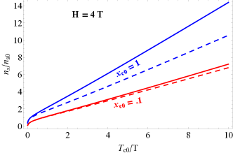
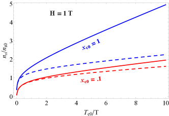
(a) (b)
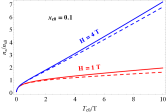
(c)

Figure 3: The CPFs density $n_{S}\left(H\right)$ (solid lines) and its approximation $n_{S}^{L}\left(H\right)$ (dashed lines) as functions of $T_{c0}/T$ (see Appendix E) for two characteristic values of the magnetic field $H$ and the cutoff parameter $x_{c0}$. (a): $H=4\boldsymbol{\mathit{T}}$; $x_{c0}=1$ (blue), $x_{c0}=0.1$ (red). (b): $H=1\boldsymbol{\mathit{T}}$ ; $x_{c0}=1$, (blue), $x_{c0}=0.1$ (red).(c): $x_{c0}=1$; $H=4\boldsymbol{\ \mathit{T}}$ (blue), $H=1\boldsymbol{\mathit{T}}$ (red). In all graphs $\widetilde{\varepsilon}_{H}$ was treated as independent parameter with the value $\widetilde{\varepsilon}_{H}=0.01$. The selected values of the basic other parameters: $T_{c0}=212$m$\boldsymbol{\mathit{K}}$ and $\varepsilon_{SO}=3\times 10^{-3}\boldsymbol{\mathit{eV}}$, yield (see Eq.67): $T_{H=4\boldsymbol{\mathit{T}}}=33$m$\boldsymbol{\mathit{K}}$. Note the asymptotic linear dependence on $T_{c0}/T$ of all graphs above certain values of $T_{c0}/T$, which depend on the values of the field $H$ and the cutoff parameter $x_{c0}$.

At low temperatures and sufficiently high fields, where $T_{H}/T\gg 1$, the asymptotic form of the digamma function yields vanishing stiffness at any finite field, i.e.:

$$\eta\left(H\right)\rightarrow\frac{T}{T_{H}},T\ll T_{H}$$ (68)

which remains finite, however, (equal to $\eta\left(0\right)=\pi^{2}/2$) at zero field.

This extreme low temperature softening of the fluctuation modes at finite field results in divergent CPFs density comm1 (see Fig.3 and more details in Appendix E):

$$n_{S}\left(H\right)\rightarrow n_{S}^{0}\left(\frac{T_{H}}{T}\right)\ln\left(1+\frac{1}{\varepsilon_{H}}\right),T\ll T_{H}$$ (69)

where the field and temperature independent CPFs density parameter $n_{S}^{0}$ is defined as:

$$n_{S}^{0}\equiv\left(\frac{7\zeta\left(3\right)E_{F}}{4\pi^{2}\hbar D}\right)\frac{1}{d}=\frac{7\zeta\left(3\right)}{2\pi}\frac{1}{d}N_{2D}\varepsilon_{SO}$$ (70)

The corresponding limiting coherence length is finite, diminishing with increasing magnetic field:

$$\xi\left(H\right)\rightarrow\frac{1}{\mu_{B}H}\sqrt{\varepsilon_{SO}\hbar D/2}=\frac{\hbar v_{F}}{2\mu_{B}H},T\ll T_{H}$$ (71)

In contrast, at zero field, the stiffness function remains finite at any temperature (i.e. $\widetilde{\eta}\left(H=0\right)=1$), and the resulting CPFs density is also finite, equal to:

$$n_{S}\left(H=0\right)=n_{S}^{0}\left(\frac{2}{\pi^{2}}\right)\ln\left(1+\frac{1}{\varepsilon}\right)$$ (72)

but with infinitely long coherence length for $T\rightarrow 0$:

$$\xi\left(H=0\right)\rightarrow\frac{1}{4}\hbar v_{F}\sqrt{\frac{\pi}{k_{B}T\varepsilon_{SO}}},T\ll T_{H}$$ (73)

It will be instructive at this point to use in Eq.60 an extension of Eq.59 for the momentum distribution function to large wavenumbers, which can be derived in the dirty limit, $\hbar/\tau_{SO}=\varepsilon_{SO}>>\mu_{B}H,k_{B}T$, i.e. (see Appendix E):

$$\left\langle\left|\phi\left(q\right)\right|^{2}\right\rangle_{H}=\frac{7\zeta\left(3\right)E_{F}}{4\pi^{2}k_{B}T}\frac{1}{\Phi\left(q;H\right)}$$ (74)

with:

$$\Phi\left(q;H\right)=\widetilde{\varepsilon}_{H}+\psi\left(\frac{1}{2}+\frac{T_{c0}}{T}\frac{2}{\pi^{2}}\xi_{0}^{2}q^{2}+\frac{T_{H}}{T}\right)-\psi\left(\frac{1}{2}+\frac{T_{H}}{T}\right)$$ (75)

and (see Eq.25):

$$\xi_{0}\equiv\xi\left(T_{c0}\right)=\sqrt{\frac{\hbar\pi D}{8k_{B}T_{c0}}}$$ (76)

Note the decorated notation $\widetilde{\varepsilon}_{H}$ used explicitly in Eq.75 for the positive-definite critical shift parameter, which was introduced originally in Ref. MZPRB2021 to take into account, self-consistently, the effect of interaction between fluctuations on $\varepsilon_{H}$ defined in Eq.42 for free (Gaussian) fluctuations. We shall use this notation for the critical shift parameter from now on in this paper to remind the reader that it can have only nonvanishing positive values, except for $T=0$, consistently with the absence of zero resistance in the experimental data.

The importance of the vanishing stiffness function, $\widetilde{\eta}\left(H\right)\simeq\left(2/\pi^{2}\right)\psi^{\prime}\left(1/2+T_{H}/T\right)\rightarrow\left(2/\pi^{2}\right)\left(T/T_{H}\right)$, of the fluctuation modes at low temperatures, $\left(T/T_{H}\right)\ll 1$, becomes transparent only after expanding the energy function, Eq.75, to first order in the kinetic energy term, which yields in agreement with Eq.59: $\Phi\left(q;H\right)\simeq\widetilde{\varepsilon}_{H}+\widetilde{\eta}\left(H\right)\left(T_{c0}/T\right)\xi_{0}^{2}q^{2}=\widetilde{\varepsilon}_{H}+\widetilde{\eta}\left(H\right)\left(\eta_{\left(2\right)}q^{2}\right)$ (see Appendix E). Continuing analytically the Taylor expansion of $\Phi\left(q;H\right)$ in $\widetilde{\eta}\left(H\right)\left(T_{c0}/T\right)\xi_{0}^{2}q^{2}\rightarrow\left(2/\pi^{2}\right)\left(T_{c0}/T_{H}\right)\xi_{0}^{2}q^{2}$, it takes the low temperature form (see Appendix E):

$$\Phi\left(q;H\right)\rightarrow\widetilde{\varepsilon}_{H}+\ln\left[1+\left(\frac{2}{\pi^{2}}\right)\left(\frac{T_{c0}}{T_{H}}\right)\xi_{0}^{2}q^{2}\right]$$ (77)

in which the logarithmic term does not depend on temperature ! The condition for the validity of the linear approximation, uniformly for all $q$ values up to the cutoff $q_{c}$:

$$\left(\frac{T_{c0}}{T_{H}}\right)x_{c0}\ll 1$$ (78)

where:

$$x_{c0}\equiv\frac{\hbar Dq_{c}^{2}}{4\pi k_{B}T_{c0}}=\frac{2}{\pi^{2}}\xi_{0}^{2}q_{c}^{2}$$ (79)

depends both on the field, through $T_{H}$, and on the cutoff wavenumber, through $x_{c0}$ (see Fig.3), but does not depend on temperature.

It is remarkable that even for larger values of the cutoff parameter $x_{c0}$, where the linear approximation (see Eq.78) is not valid, the low temperature (asymptotic) CPFs density, given by:

$$n_{S}\left(H\right)\rightarrow n_{S}^{0}\left(\frac{T_{H}}{T}\right)\int_{0}^{x_{c0}T_{c0}/T_{H}}\frac{d\chi}{\widetilde{\varepsilon}_{H}+\ln\left(1+\chi\right)}$$ (80)

has the same $1/T$ divergence at $T\ll T_{H}$ as the linear approximation given by Eq.69, but with a larger slope, as shown in Fig.3 (see also Appendix E).

V.2 The crossover to localization and phase separation of Cooper-pair fluctuations

The discontinuous nature of the stiffness function $\eta\left(H\right)$ at $H=0$ in the zero-temperature limit, revealed in Eq. 68, is inherent to peculiar features of the CPFs at low temperatures. These features may be best appreciated by considering the Fourier transform to real space of the momentum distribution function, Eq.59, in the low temperature limit $T\ll T_{H}$, where field-induced condensation in real space is expected on the basis of the limiting behavior of $n_{S}\left(H\right)$ and $\xi\left(H\right)$ according to Eqs.69 and 71, respectively. This Fourier transform is related to the Cooper-pairs amplitude correlation function (that is proportional to the static fluctuation propagator in real space), through the equation:

$$\left\langle\phi^{\ast}\left(\mathbf{r}\right)\phi\left(\mathbf{r}+\boldsymbol{\rho}\right)\right\rangle_{H}=\left(\frac{1}{2\pi}\right)^{2}\int d^{2}q\left\langle\left|\phi\left(q\right)\right|^{2}\right\rangle_{H}e^{i\boldsymbol{q\cdot\rho}}$$ (81)

in which we may use the more general expression for the momentum distribution function in the dirty limit, Eq.74, i.e. with $\Phi\left(q;H\right)$ given by Eq.75. Performing the angular integration in Eq.81 it can be rewritten in the form:

$$\left\langle\phi^{\ast}\left(\mathbf{r}\right)\phi\left(\mathbf{r}+\boldsymbol{\rho}\right)\right\rangle_{H}=\frac{1}{2\pi}n_{S}^{0}\xi_{0}^{-2}g\left(\rho/\xi_{0}\right)$$ (82)

where $g\left(\rho/\xi_{0}\right)$ is given by:

$$g\left(\rho/\xi_{0}\right)=\frac{T_{c0}}{T}\int_{0}^{\widetilde{q}_{c}}\frac{\widetilde{q}J_{0}\left(\widetilde{q}\rho/\xi_{0}\right)}{\Phi\left(\widetilde{q};H\right)}d\widetilde{q}$$ (83)

$\widetilde{q}\equiv\xi_{0}q$, and $J_{0}\left(\widetilde{q}\rho/\xi_{0}\right)$ is the zero order Bessel function of the first kind.

The correlation function $g\left(\rho/\xi_{0}\right)$ is proportional to the probability amplitude for a CPF to propagate a distance $\rho=\left|\boldsymbol{\rho}\right|$ from any point $\mathbf{r}$. Its dependence on $\rho$ has a decaying envelope, modulated by an oscillatory function associated with the sharp cutoff $q_{c}$. The length scale of this attenuation is the localization length, given by (see Appendix F):

$$\rho_{loc}\left(H\right)=\left(\frac{T_{c0}}{T}\frac{\widetilde{\eta}\left(H\right)}{\widetilde{\varepsilon}_{H}}\right)^{1/2}\xi_{0}$$ (84)

The results of a detailed analysis of the correlation function $g\left(\rho/\xi_{0}\right)$ and its asymptotic behavior (see Appendix F) are shown in Fig.4, where the condensing CPFs are found to localize within a region of diminishing size of the order of $\rho_{loc}\left(H\right)$ under increasing field $H$. The positive-definite self-consistent critical shift parameter, $\widetilde{\varepsilon}_{H}$, appearing in Eq.84, which is a monotonically increasing function of the field $H$, is used in the calculations as an independent free parameter, in order to illustrate how the minimal gap, $\widetilde{\varepsilon}_{H}$, of the energy spectrum given in Eq.75, influences the condensation and localization of CPFs in real space.

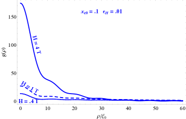
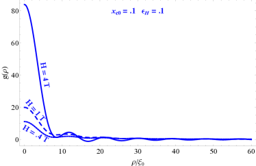
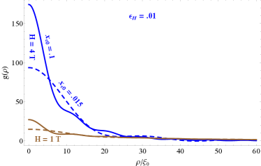
(a) (b)
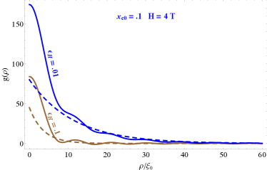
(c) (d)

Figure 4: Dimensionless real-space CPFs density $g\left(\rho/\xi_{0}\right)$, illustrating the phenomena of condensation and localization of CPFs, as discussed in the text, calculated at temperature $T=2$mK for different values of the magnetic field, $H$ , the cutoff parameter $x_{c0}$, and $\widetilde{\varepsilon}_{H}$, which is considered for illustration as independent free parameter. (a) $x_{c0}=.1$; $\widetilde{\varepsilon}_{H}=.01$; $H=4$T,$1$T,$.1$T. (b) $x_{c0}=.1$ ;$\widetilde{\varepsilon}_{H}=.1$ ; $H=4$T,$1$T,$.1$T. (c) $x_{c0}=.1$; $H=4$T ; $\widetilde{\varepsilon}_{H}=.01$(blue), $\widetilde{\varepsilon}_{H}=.1$(brown), exponential asymptotes (dashed lines) (see Appendix F). (d) $\widetilde{\varepsilon}_{H}=.01$; $x_{c0}=.1$ (solid lines), $x_{c0}=.015$ (dashed lines); $H=4T$ (blue), $H=1T$ (brown).

The physical implications of this phenomenon are far reaching; in particular, condensation of the charged CPFs in restricted 2D spatial regions (puddles) drives the unpaired, normal-state electrons, due to Coulomb repulsion, away from the puddles’ centers into inter-puddel regions, resulting in phase separation between the two charged subsystems during CPF life-time. The crossover from a spatially uniform (gas) of CPFs, at zero field, to mesoscopic puddels of condensed CPFs takes place at fields $H\sim H_{cross}$, where:

$$\widetilde{\eta}\left(H_{cross}\right)=1/2$$

(see Fig.5a). At low temperatures, where $T\ll T_{H}$, the crossover field, $H_{cross}$, may be estimated by using Eq.68, which yields:

$$\mu_{B}H_{cross}\sim\left(\varepsilon_{SO}k_{B}T\right)^{1/2}$$ (85)

For the sake of better sense of scaling, we may estimate the field, $H_{upp}$ at which the low-temperature limit of the CPFs density $n_{S}\left(H\right)$, Eq.69, approaches its (physical) upper limit, i.e. $1/2$ of the total number density of electrons $n_{0}=k_{F}^{2}/2\pi d$:

$$n_{S}\left(H\right) \rightarrow \left(\frac{7\zeta\left(3\right)}{4\pi^{2}}\right)\frac{1}{d}N_{2D}\frac{\left(\mu_{B}H\right)^{2}}{k_{B}T}\ln\left(1+\frac{1}{\widetilde{\varepsilon}_{H}}\right)$$

$$= \frac{1}{2}\left(\frac{1}{d}\frac{k_{F}^{2}}{2\pi}\right)=\frac{1}{2}n_{0}$$

which yields:

$$\mu_{B}H_{upp}\sim\left(E_{F}k_{B}T\right)^{1/2}$$ (86)

Thus, the plausible hierarchy of the parameters $E_{F}>\varepsilon_{SO}$ ensures that the crossover field, $H_{cross}$ can always be reached.

VI Discussion and Conclusion

The peculiar features of the system of CPFs, discussed in the previous sections, reflect essential inconsistency of the microscopic theory of fluctuations in superconductors at finite field and very low temperatures. In particular, it was shown that the contribution of the basic pair of diagrams to the DOS conductivity obtained within the conventional microscopic approach can be expressed in terms of an effective Drude formula (see Eq.63) in which $n_{S}\left(H\right)$ is an effective CPFs density (Eq.60) and $\tau_{SO}\left(H\right)$ is an effective single electron relaxation time (Eq.64). These definitions are not arbitrary; the field dependence of $\tau_{SO}\left(H\right)$ is exclusively determined by the renormalized pairing vertex factors (see Eq.51), associated with electron scatterings by background electrons via virtual exchange of CPFs.

On the other hand, the field dependence of $n_{S}\left(H\right)$ is associated exclusively with the fluctuation propagator, controlled by the stiffness function $\widetilde{\eta}\left(H\right)$, which tends to zero at any $H>0$ with $T\rightarrow 0$ (see Eq.68), but remains finite (equal to $1$) at zero field. Consequently, the density $n_{S}\left(H\right)$ diverges for $T\rightarrow 0$ at any $H>0$ (see Eq.69 and note the comment in Ref.comm1 ), but remains finite at $H=0$ (see Eq.72). Furthermore, the divergent Cooper-pair coherence length $\xi\left(H=0\right)$ in the $T\rightarrow 0$ limit (Eq.73), which characterizes a homogeneous system at $H=0$, contracts at $H>0$ to a finite length, where increasingly large numbers of CPFs condense under diminishing temperature.

The state-of-the-art microscopic theory of fluctuations in superconductors which leads to these peculiar results is basically a perturbation theory, developed for spatially homogenous systems, which rests upon a diagrammatic expansion of the conductivity in the fluctuations propagator about the normal-state conductivity. In this framework the scope of the calculations is restricted to fluctuations in the normal-state conductivity above the transition to superconductivity. Within this microscopic approach we may write the total conductivity as:

$$\sigma_{tot}^{mic}\left(H\right)=\sigma_{n}+\sigma_{DOS}^{mic}\left(H\right)+\sigma_{AL}^{mic}\left(H\right)$$ (87)

where $\sigma_{n}$ is the normal-state (zero-order in the expansion) conductivity, $\sigma_{DOS}^{mic}\left(H\right)$ is the DOS conductivity given by Eq.65, and $\sigma_{AL}^{mic}\left(H\right)$ is the AL conductivity written in Eq.45.  As indicated in Sec.III, the Maki-Thompson conductivity (MakiPTP1968 ,ThompsonPRB1970 ) is neglected here due to the presence of strong spin-orbit scatterings (see Appendix A). It should be emphasized that both $\sigma_{DOS}^{mic}\left(H\right)$ and $\sigma_{AL}^{mic}\left(H\right)$ have been calculated here within the framework of the LV method used in Ref.LV05 in which quantum critical fluctuations were neglected.

Under these circumstances at finite field $H$ and very low temperature $T\ll T_{H}$, due to the vanishing $\widetilde{\eta}\left(H\right)\rightarrow\left(2/\pi^{2}\right)T/T_{H}$ and the more quickly vanishing $\widetilde{\tau}_{SO}\left(H\right)\rightarrow\left(T/T_{H}\right)^{2}/7\zeta\left(3\right)$, both the AL (Eq.45) and DOS (Eq.65) conductivities:

$$\sigma_{AL}^{mic}\left(H\right) \rightarrow \frac{e^{2}}{8\pi^{2}d\hbar}\left(\frac{T}{T_{H}}\right)\frac{1}{\widetilde{\varepsilon}_{H}},$$ (88)

$$\sigma_{DOS}^{mic}\left(H\right) \rightarrow -\frac{e^{2}}{2\pi^{2}d\hbar}\left(\frac{T}{T_{H}}\right)\ln\left(\frac{1}{\widetilde{\varepsilon}_{H}}\right)$$ (89)

vanish with $T$.  This linearly vanishing with temperature AL and DOS conductivities are consistent with the results reported in Ref.Glatzetal2011 at very low temperatures in the absence of quantum critical fluctuations (see a remark below Eq.9). The different field dependencies should be related to the different magnetic field orientations (perpendicular in Ref.Glatzetal2011 as compared to parallel in our case).

The above discussion clearly indicates that this perturbation theory can not be directly applied to the extremely inhomogeneous real-space Cooper-pairs (boson) condensate that emerges from our analysis. In particular, although the leading-order (i.e. the DOS and the AL) diagrams contribution to the fluctuation conductivity vanishes for $H>0,T\rightarrow 0$, the definition of the (zeroth order) normal-state conductivity should be drastically modified by the (divergent) CPFs density $n_{S}\left(H\right)$. Indeed, the localization of CPFs in mesoscopic puddles under increasing field and diminishing temperature, discussed above, indicates that they may be regarded as long-lived collective charged excitations, which should phase separate by Coulomb repulsion from their source system of normal (unpaired) electrons. This system of normal-state electrons, which are restricted to regions of diminishing scatterings by CPFs, holds, however, interphase dynamical equilibrium, via charge exchange, with the puddles of CPFs during their life-times.

Thus, formally speaking, while using the simple Drude expression $\left(e^{2}/m^{\ast}\right)n_{0}\tau_{n}$ for $\sigma_{n}$ in Eq.87 with $\tau_{n}$– the normal-state electron relaxation time (equal in our model to $\tau_{SO}$), one notes that it is valid only under the usual situation of nearly uniform real-space distribution of CPFs. However, under the unusually inhomogeneous situation, outlined above, of divergent number density $n_{S}\left(H\right)$ of CPFs in mesoscopic puddles, their dynamical equilibrium with the normal-state electrons should lead, under the assumption of a fixed total number of electrons, to the following modification:

$$\sigma_{n}\rightarrow\sigma_{n}^{Mod}\left(H\right)=\frac{e^{2}}{m^{\ast}}n_{0}\tau_{SO}-\frac{e^{2}}{m^{\ast}}2n_{S}\left(H\right)\tau_{SO}$$ (90)

The total consumption of electrons in the process of pairing sets an upper bound on $n_{S}\left(H\right)$, i.e. $2n_{S}\left(H\right)\leq n_{0}$, corresponding to the ultimate vanishing of $\sigma_{n}\left(H\right)$ for $H>0,T\rightarrow 0$, that is physically equivalent to infinite high-field MR.

This ultimate vanishing of both the fluctuation and the normal-state conductivities in the zero temperature limit is due to our neglect of quantum fluctuations. As discussed in detail in several recent papers (Glatzetal2011 , Lopatinetal05 , Khodas2012 ), corrections due to quantum fluctuations in both the DOS and the AL conductivities (as well as in Maki-Thompson contributions, neglected here, see Appendix A) around the quantum critical field prevent the vanishing of the fluctuation conductivity in the zero temperature limit. Furthermore, as discussed in Ref.MZPRB2021 ,MZJPC2023 , quantum tunneling fluctuations (see below) suppress the divergent CPFs density and so prevent the vanishing of $\sigma_{n}^{Mod}\left(H\right)$ in Eq.90.

In the less extreme situations of finite fields and low temperatures, above the crossover field, Eq.85, the second term on the RHS of Eq.90 is identified with the DOS conductivity derived within our TDGL functional approach. Thus, as long as $\widetilde{\tau}_{SO}\left(H\right)\ll 1$, the result of replacing $\sigma_{n}$ in Eq.87 with $\sigma_{n}^{Mod}\left(H\right)$ is seen to agree with the expression for the total conductivity derived within our TDGL functional approach MZJPC2023 .

The crucial point here is in the existence of phase separated condensed mesoscopic puddles of long-lived boson excitations, which act through pair-breaking processes as reservoirs for (unpaired) conduction electrons. Within this picture the conductance of the boson excitations is exclusively represented by the Schmidt-Fulde-Maki paraconductivity (see Eq.14), shown above to be equivalent to the Aslamozov-Larkin conductivity in the microscopic diagrammatic approach. On the other hands, the remaining system of unpaired electrons, restricted to regions of diminishing scattering by CPFs, keeps its normal-state relaxation time $\tau_{SO}$, so that its conductance is influenced by the Cooper-pair bosons only through interphase charge exchange, as expressed in Eq.90.

The resulting expression for the total conductance, for $T\ll T_{H}$, $H\geq H_{cross}$:

$$\sigma_{tot}\left(H\right)\rightarrow\sigma_{n}\left(H\right)-2\frac{e^{2}}{m^{\ast}}n_{S}\left(H\right)\tau_{SO}+\sigma_{AL}\left(H\right)$$ (91)

includes a well defined normal-state conductivity, $\sigma_{n}\left(H\right)$, which is now completely independent of the pairing effect. Its field dependence is introduced to account for possible normal-state MR effects, such as weak localization etc…Hikami-etal-PTP1980 , Fukuyama1985 .

The validity of Eq.91 is bound to a complete phase separation between the negatively charged clouds of the CPFs puddles and the unpaired electrons, which can be realized at sufficiently high field and low temperature below $T_{H}$. However, under lowering field and/or elevating temperature, increasing overlap between the clouds, following increasing smearing of the CPFs puddles, which leads eventually to their evaporation into a uniform gas of CPFs, bring the system back to conditions of a spatially uniform 2D electron gas perturbed by CPFs, for which the conventional microscopic perturbation theory should hold. In the corresponding expression for the conductivity, Eq.87, with $\sigma_{DOS}^{mic}\left(H\right)$ given by Eq.65, the single electron relaxation time $\tau_{SO}\left(H\right)$ is close to that of the normal-state value $\tau_{SO}$, so that: $\sigma_{tot}\left(H\right)\rightarrow\sigma_{n}-4\left(e^{2}/m^{\ast}\right)n_{S}\left(H\right)\tau_{SO}+\sigma_{AL}\left(H\right)$.

In the intermediate fields range a more complete theory, which takes into account the smearing of the CPFs puddles and the overlap of their extending tails with the unpaired electrons cloud, would introduce corrections to the conductivity, interpolating between the high and low-field asymptotes. A plausible heuristic expression for such an interpolation function, assigned effectively to the DOS conductivity contribution in Eq.87, would take the form:

$$\sigma_{DOS}^{eff}\left(H\right)=-2\frac{e^{2}}{m^{\ast}}n_{S}\left(H\right)\overline{\tau}_{SO}\left(H\right)$$ (92)

where the effective electron relaxation time is defined by:

$$\overline{\tau}_{SO}\left(H\right)\equiv 2\widetilde{\eta}\left(H\right)\tau_{SO}\left(H\right)+\left[1-\widetilde{\eta}\left(H\right)\right]\tau_{SO}$$ (93)

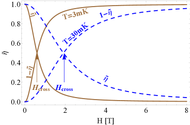
(a)
(b)

Figure 5: (a): The coefficients $\widetilde{\eta}\left(H\right)$ and its complement $\left[1-\widetilde{\eta}\left(H\right)\right]$ representing the relative weights of the smearing effect of the CPFs mesoscopic puddles and of their tendency to phase separate, respectively, as functions of the field $H$, for two different temperatures. The corresponding crossover fields $H_{cross}$ are indicated. (b): The effective single-electron relaxation time $\overline{\tau}_{SO}\left(H\right)$, calculated according to Eq.93 for the same parameters used in (a). Note the proximity of $\overline{\tau}_{SO}\left(H\right)$ to the free-electron value $\tau_{SO}$, which characterizes the TDGL approach, in the main fields range above $H=0$.

Here, the coefficients $\widetilde{\eta}\left(H\right)$ and $\left[1-\widetilde{\eta}\left(H\right)\right]$ represent, respectively, the relative weights of the smearing effect of the CPFs mesoscopic puddles, and of their tendency to phase separate, in evaluating the effective electron relaxation time. Indeed, as shown in Fig.5, the normalized stiffness function $\widetilde{\eta}\left(H\right)$ increases from $0$ to $1$ upon increasing smearing, whereas its complement $\left[1-\widetilde{\eta}\left(H\right)\right]$ sets a measure, between $1$ and $0$, of the CPFs puddles integrity. Thus, the two-edge situations of Eq.93, mentioned above, are easily understood: For $\widetilde{\eta}\left(H\right)\approx 1$, where the overlap between CPFs and electron clouds is nearly complete, so that the single-electron relaxation time is fully influenced by CPFs-scatterings, we have: $\overline{\tau}_{SO}\left(H\right)\approx 2\tau_{SO}\left(H\right)\approx 2\tau_{SO}$, whereas for $\widetilde{\eta}\left(H\right)\approx 0$, where phase separation is nearly complete, one finds: $\overline{\tau}_{SO}\left(H\right)\approx\tau_{SO}$. Note the doubling of $\overline{\tau}_{SO}\left(H\right)$, with respect to $\tau_{SO}$, in the complete overlap limit, which reflects its different definition as compared to $\tau_{SO}\left(H\right)$.

The crossover field $H_{cross}$ (see Eq.85) determines the balance between the two competing tendencies: In the low-fields region $H\ll H_{cross}$, where both $\widetilde{\tau}_{SO}\left(H\right)$ and $\widetilde{\eta}\left(H\right)\rightarrow 1$, one finds the conventional microscopic result, $\sigma_{tot}\left(H\right)=\sigma_{n}-4\left(e^{2}/m^{\ast}\right)n_{S}\left(H\right)\tau_{SO}+\sigma_{AL}\left(H\right)$, whereas in the high-fields region $H\gg H_{cross}$, where both $\widetilde{\tau}_{SO}\left(H\right)$ and $\widetilde{\eta}\left(H\right)\ll 1$, one finds the limiting TDGL result, Eq.91.  We therefore conclude that at sufficiently low temperatures, where $T\ll T_{H_{cross}}$, the TDGL approach is valid in the entire fields range except for the small region $H\leq H_{cross}=\left(\varepsilon_{SO}k_{B}T\right)^{1/2}/\mu_{B}$ (see Fig.5b).

The picture of charged boson condensates, phase separated from normal-electron regions, which hold mutual dynamical equilibrium, via charge exchange, leads one naturally to expect that quantum tunneling of CPFs should take place across GL energy barriers, built-up on puddles’ boundaries. Of course, this should be followed by a certain pair-breaking process to sustain the charge exchange across the barriers. The combined tunneling-pair-breaking process should be, therefore, responsible for suppressing the divergent $n_{S}\left(H\right)$ at $T\rightarrow 0$, under the condition of total charge conservation, such that:

$$\lim_{T\rightarrow 0}2n_{S}^{QTPB}\left(H\right)\leq n_{0}\left(H\right)=\left(m^{\ast}/\tau_{SO}e^{2}\right)\sigma_{n}\left(H\right)$$

We have presented in our previous papers MZPRB2021 ,MZJPC2023 a phenomenological approach to account for these quantum processes. Their underlying microscopic quantum dynamics remains a demanding challenge in the GL theory.

The influence of quantum critical fluctuations on the AL and DOS conductivities at finite field in the zero temperature limit has been evaluated within the conventional microscopic theory, both for parallel (Lopatinetal05 , Khodas2012 ) and perpendicular (Glatzetal2011 ) field orientations. Typically, it has been found to introduce corrections to the vanishing ”classical” results of magnitude similar to (see e.g. Glatzetal2011 ):

$$\delta\sigma_{xx}^{Q}\left(H\right)=-\frac{2e^{2}}{3\pi^{2}d\hbar}\ln\left(\frac{1}{\widetilde{\varepsilon}_{H}}\right)$$ (94)

These corrections have been found, however, to be too small for sufficiently influencing the normal-state conductivity in any attempt to account for the pronounced MR peaks observed experimentally in Ref.Mograbi19 . In contrast, at sufficiently low temperatures $T\ll T_{H_{cross}}$, the effective DOS conductivity, Eq.92, which takes the divergent form:

$$\sigma_{DOS}^{eff}\left(H\right)\sim-\frac{3.5\zeta\left(3\right)e^{2}}{\pi^{2}d\hbar}\left(\frac{T_{H}}{T}\right)\ln\left(\frac{1}{\widetilde{\varepsilon}_{H}}\right)$$ (95)

is in principle capable of producing the observed large MR peaks, their actual intensities depend, however, on the quantum tunneling effect discussed above.

In conclusion, promoting the hypothesis that the large MR observed at low temperatures, just above a crossover field to superconductivity, in the electron-doped SrTiO₃/LaAlO₃ interfaces Mograbi19 ,RoutPRL2017 , is associated with CPFs, it is shown that the state-of-the-art microscopic theory of fluctuations in superconductors fails to account for this remarkable effect. This failure is attributed here to the restrictive nature of this theory which is limited to expansions about homogeneous electron systems.

A proper definition of the density of CPFs within this microscopic theory shows, however, that at sufficiently low temperatures the pairing process under increasing field becomes unstable with respect to formation of mesoscopic puddles of condensed CPFs, so that, due to Coulomb repulsion, the puddles of charged CPFs are phase separated from the underlying (unpaired) normal-state electron gas. The strongly enhanced MR therefore arises from charge transfer, under dynamical equilibrium, between the condensing CPFs, localized in mesoscopic puddles, and rarefying unpaired normal-state electron gas.

Appendix A The relevant diagrams

The literature dealing with the effect of superconducting fluctuations on the conductivity from the point of view of the microscopic GGL theory is quite extensive. The most comprehensive and elaborated account of this approach can be found in Ref.LV05 . Some specific details relevant to our analysis of the diagrams shown in Fig.1, concerning in particular, the relative importance of the various contributions to the DOS conductivity (diagrams 5-8 in Fig.1), can be found in earlier papers: AltshulerJETP1983 , Dorin-etal-PRB1993 .

A different type of diagrams (2-4 in Fig.1), corresponding to electron-hole (Andreev-like) scatterings by CPFs ManivAlexanderJPC1976 , that is well-known as the Maki–Thompson diagram MakiPTP1968 ,ThompsonPRB1970 , includes two parts of contributions: A singular part, arising from the coherent Andreev-like scattering, with positive contribution to the fluctuation conductivity, and a regular part with negative contribution to the conductivity, similar to the DOS conductivity. In our model we disregard this type of diagrams altogether since the strong spin-orbit scatterings, which characterize the SrTiO₃/LaAlO₃ interfaces under consideration here, are known to destroy the coherence responsible for the singularity LV05 , so that the remaining regular positive contribution is cancelled, or nearly cancelled by the negative ones ManivAlexanderJPC1977 .

Appendix B The Copper-pairs (GL) current density

Eq.12 is obtained from the variational condition of the electromagnetically modified GL free energy functional with respect to the vector potential:

$$\frac{\partial\mathfrak{L}\left(\Delta,\mathbf{A}\right)}{\partial\mathbf{A}}+\frac{1}{8\pi}\frac{\partial}{\partial\mathbf{A}}\int d^{3}r\left(\mathbf{\nabla}\times\mathbf{A}\right)^{2}=0$$ (96)

in conjunction with the identity:

$$\frac{1}{8\pi}\frac{\partial}{\partial\mathbf{A}}\int d^{3}r\left(\mathbf{\nabla}\times\mathbf{A}\right)^{2}=\frac{1}{4\pi}\mathbf{\nabla}\times\left(\mathbf{\nabla}\times\mathbf{A}\right)=\frac{1}{c}\mathbf{j}$$

Appendix C The normalization constant

To find $\alpha$ we note that Eq.23, relating the propagators, $\mathcal{D}\left(q,\Omega\right)$ in the $\Delta$ representation to $L\left(q,\Omega\right)$ in the $\phi$ representation, is equivalent to the normalization of the GL wavefunction:

$$\left|\phi\left(\mathbf{r}\right)\right|^{2}=\frac{N_{2D}}{\left(\alpha k_{B}T\right)}\left|\Delta\left(\mathbf{r}\right)\right|^{2}$$ (97)

As emphasized in the main text, the normalization constant $\alpha$, in the dirty-limit under study, may be evaluated in the clean limit, i.e. for coherence length:

$$\xi\left(T\right)\rightarrow\xi_{c}\left(T\right)=\sqrt{\frac{7\zeta\left(3\right)}{8}}\left(\frac{\hbar v_{F}}{2\pi k_{B}T}\right)$$ (98)

since normalization of the wavefunctions should not depend on scatterings. Thus, using the expression for $\alpha$ presented in Eq.29, for which the normalization takes the form:

$$\left|\phi\left(\mathbf{r}\right)\right|^{2}=\frac{7\zeta\left(3\right)}{8}\frac{k_{F}^{2}}{2\pi}\left(\frac{\left|\Delta\left(\mathbf{r}\right)\right|}{\pi k_{B}T}\right)^{2}\simeq\frac{k_{F}^{2}}{2\pi}\left(\frac{\left|\Delta\left(\mathbf{r}\right)\right|}{\pi k_{B}T}\right)^{2}$$ (99)

the clean-limit GL propagator, Eq.24, at zero frequency, is written in the canonical Schrodinger-like form:

$$L\left(q,0\right)^{-1}=\frac{\hbar^{2}}{4m^{\ast}}\left[\xi\left(T\right)^{-2}\varepsilon+q^{2}\right]$$ (100)

with the Cooper-pair mass equals twice the electron band mass $m^{\ast}$.

The dirty-limit momentum distribution function, Eq.26, may be therefore evaluated with $\alpha$ given by Eq.29 with the dirty-limit coherence length given in Eq.25.  The result takes the form:

$$\left\langle\left|\phi\left(q\right)\right|^{2}\right\rangle=\frac{28\zeta\left(3\right)}{\pi^{2}}\left(N_{2D}\frac{\hbar}{\tau_{SO}}\right)\frac{1}{\xi\left(T\right)^{-2}\varepsilon+q^{2}}$$ (101)

with the dirty limit coherence length:

$$\xi\left(T\right)\rightarrow\xi_{d}\left(T\right)=\sqrt{\frac{\pi\hbar D}{8k_{B}T}}$$ (102)

For comparison, the clean limit result is obtained from Eq.101 by replacing $\hbar/\tau_{SO}$ with $\left[4\pi^{3}/7\zeta\left(3\right)\right]k_{B}T$ and $\xi_{d}\left(T\right)$ with $\xi_{c}\left(T\right)$ for the coherence length $\xi\left(T\right)$.

Finally, the TDGL expression for the DOS conductivity, defined in terms of the CPFs density $n_{s}$ by using using Eq.101, is shown here to coincide with the basic microscopic (diagrammatic) result, that is:

$$\sigma_{DOS}^{TDGL}\equiv-2n_{s}\frac{e^{2}}{m^{\ast}}\tau_{SO}\equiv$$

$$-\frac{e^{2}}{\hbar d}\frac{7\zeta\left(3\right)}{\pi^{4}}\int\frac{d\left(\xi\left(T\right)^{2}q^{2}\right)}{\varepsilon+\xi\left(T\right)^{2}q^{2}}=\sigma_{xx}^{LV\left(5+7\right)}$$ (103)

Appendix D The dispersion suppressed zero-field DOS conductivity

Consider the corrected zero-field DOS conductivity, Eq.31 , which includes the $q$ dependence of the single-electron relaxation time $\tau_{SO}\left(q\right)$, that is:

$$\sigma_{DOS}^{LV,corr}=\frac{e^{2}}{2\pi^{4}}\frac{1}{\hbar d}\int_{0}^{1}dx\psi^{\prime\prime}\left(\frac{1}{2}+\frac{2}{\pi^{2}}x\right)\frac{1}{\varepsilon+x}$$

where $x=\pi\hbar Dq^{2}/8k_{B}T$, and: $\psi^{\prime\prime}\left(1/2+2x/\pi^{2}\right)=-2\sum\limits_{n=0}^{\infty}\left(n+1/2+2x/\pi^{2}\right)^{-3}$.  The result is nonvanishing negative function of $\varepsilon$ ($0<\varepsilon\ll 1$), which may be estimated, using two-parameter fitting scheme, to be:

$$\sigma_{DOS}^{LV,corr}\approx-\left(\frac{1}{2\pi^{4}}\right)\left(\frac{e^{2}}{d\hbar}\right)\left[7\ln\left(1+\frac{1}{\varepsilon}\right)-1\right]$$ (104)

It shows that the $q$ dispersion of $\tau_{SO}\left(q\right)$ suppresses the magnitude of $\sigma_{DOS}^{LV}$ to about $1/2$ of Eq.33

Appendix E The CPFs density

An expression for the CPFs density in terms of a generalized form of the fluctuation energy function $\Phi\left(q;H\right)$, which is valid at large wavenumbers, is given by (see Ref.MZJPC2023 ):

$$n_{S}\left(H\right)=\left(\frac{7\zeta\left(3\right)E_{F}}{4\pi^{2}k_{B}T}\right)\frac{\pi}{d}\int_{0}^{q_{c}^{2}}\frac{d\left(q^{2}\right)}{\left(2\pi\right)^{2}}\frac{1}{\Phi\left(q;H\right)}$$

where:

$$\Phi\left(q;H\right)=\varepsilon_{H}+a_{+}\left[\psi\left(\frac{1}{2}+f_{-}+x\right)-\psi\left(\frac{1}{2}+f_{-}\right)\right]$$

$$+a_{-}\left[\psi\left(\frac{1}{2}+f_{+}+x\right)-\psi\left(\frac{1}{2}+f_{+}\right)\right]$$ (105)

and $x=\hbar Dq^{2}/4\pi k_{B}T$.  Note the use of the general expression, Eq.105, for the dimensionless energy $\Phi\left(q;H\right)$ under the integral for $n_{S}\left(H\right)$, with the field-independent kinetic energy variable $x$, suggesting that the cutoff wavenumber $q_{c}$ should also be field independent.

Under the dirty limit condition: $\hbar/\tau_{SO}=\varepsilon_{SO}>>\mu_{B}H$, one finds for $f_{\pm}=\frac{\varepsilon_{SO}}{4\pi k_{B}T}\left(1\pm\sqrt{1-\left(\frac{2\mu_{B}H}{\varepsilon_{SO}}\right)^{2}}\right)$:

$$f_{+}\simeq\frac{\varepsilon_{SO}}{4\pi k_{B}T}\left[1+\left(1-2\left(\frac{\mu_{B}H}{\varepsilon_{SO}}\right)^{2}\right)\right]\simeq\frac{\varepsilon_{SO}}{2\pi k_{B}T},$$

$$f_{-}\simeq\frac{\varepsilon_{SO}}{4\pi k_{B}T}\left[1-\left(1-2\left(\frac{\mu_{B}H}{\varepsilon_{SO}}\right)^{2}\right)\right]\simeq$$

$$\frac{\varepsilon_{SO}}{2\pi k_{B}T}\left(\frac{\mu_{B}H}{\varepsilon_{SO}}\right)^{2}<<f_{+}$$

, and for $a_{\pm}$: $a_{+}\simeq 1,a_{-}\simeq\left(\frac{\mu_{B}H}{\varepsilon_{SO}}\right)^{2}<<1$, so that:

$$\Phi\left(q;H\right)\simeq\Phi\left(x,\frac{T_{H}}{T}\right)\equiv\varepsilon_{H}+\psi\left(\frac{1}{2}+x+\frac{T_{H}}{T}\right)-\psi\left(\frac{1}{2}+\frac{T_{H}}{T}\right)$$ (106)

where $T_{H}$ is given in Eq.67.

The linear approximation:

$$\Phi\left(x,\frac{T_{H}}{T}\right) \simeq \Phi_{L}\left(x,\frac{T_{H}}{T}\right)=\varepsilon_{H}+\psi^{\prime}\left(\frac{1}{2}+\frac{T_{H}}{T}\right)x$$ (107)

$$\simeq\varepsilon_{H}+\eta\left(H\right)x$$

is identical to the energy denominator of the fluctuation propagator in Eq.41.

The exact expression for the CPFs density is, then, written in the form:

$$n_{S}\left(H\right)=n_{S}^{0}\int_{0}^{x_{c0}T_{c0}/T}\frac{dx}{\Phi\left(x,\frac{T_{H}}{T}\right)}$$ (108)

where $n_{S0}$ is given in Eq.70.

Performing the integration in Eq.108 with $\Phi\left(x,T_{H}/T\right)$ replaced by the linear approximation $\Phi_{L}\left(x,T_{H}/T\right)$ we find for the linear approximation of the CPF density:

$$n_{S}^{L}\left(H\right)=\frac{n_{S}^{0}}{\psi^{\prime}\left(\frac{1}{2}+\frac{T_{H}}{T}\right)}\ln\left(1+\frac{\widetilde{x}_{c}\left(H\right)}{\varepsilon_{H}}\right)$$ (109)

where:

$$\widetilde{x}_{c}\left(H\right)\equiv\psi^{\prime}\left(\frac{1}{2}+\frac{T_{H}}{T}\right)\left(\frac{T_{c0}}{T}\right)x_{c0}$$

Using the asymptotic form of the digamma function for the low temperature limit $T/T_{H}\ll 1$ we find:

$$n_{S}^{L}\left(H\right) \rightarrow \left(\frac{T_{H}}{T}\right)n_{S}^{0}\ln\left(1+\frac{\widetilde{x}_{c}\left(H\right)}{\varepsilon_{H}}\right),$$ (110)

$$\widetilde{x}_{c}\left(H\right) \rightarrow \left(\frac{T_{c0}}{T_{H}}\right)x_{c0}$$

which is identical to Eq.69, provided $\widetilde{x}_{c}\left(H\right)$ is selected to be field independent, e.g.: $\widetilde{x}_{c}\left(H\right)\rightarrow 1$. The latter selection is consistent with the selection of the cutoff wavenumber to depend on field according to: $q_{c}=\xi^{-1}\left(H\right)$ (see Eq.61 and text around Eq.65).

We note that in our fitting procedure, employed in Refs.MZPRB2021 , MZJPC2023 , we have used the field-independent cutoff selection for $q_{c}$. Specifically, the best fitting value was found to agree with $x_{c0}=0.015$ (see Eq.79) with the selected values of the other parameters: $T_{c0}=0.212\boldsymbol{\mathit{K}}$ and $\varepsilon_{SO}=3\times 10^{-3}\boldsymbol{\mathit{eV}}$.

As indicated in the main text, deviations from the linear approximation may be significant for large cutoff wavenumbers which do not satisfy condition 78. Under these circumstances and in the low temperatures region, $T/T_{H}\ll 1$, we may use the asymptotic form of the digamma functions in Eq.106, which can be rewritten as: $\Phi\left(x,\frac{T_{H}}{T}\right)\rightarrow\varepsilon_{H}+\ln\left(x+T_{H}/T\right)-\ln\left(T_{H}/T\right)=\varepsilon_{H}+\ln\left(1+xT/T_{H}\right)$, that is:

$$\Phi\left(x,\frac{T_{H}}{T}\right) \rightarrow \varepsilon_{H}+\ln\left(1+\frac{\hbar Dq^{2}}{4\pi k_{B}T_{H}}\right),$$ (111)

$$T/T_{H} \ll 1$$

In Fig.3 we plot $n_{S}\left(H\right)$ using Eq.108 with the exact expression, Eq.106, for $\Phi\left(x,T_{H}/T\right)$, together with $n_{S}^{L}\left(H\right)$ given in Eq.109, as functions of $T_{c0}/T$ for different values of the field $H$ and cutoff parameter $x_{c0}$.

Appendix F CPFs localization length

Starting with Eq.83 for the correlation function $g\left(\rho/\xi_{0}\right)$ we will be interested here in its asymptotic behavior for $\rho/\xi_{0}\gg 1$, which will enable us to clearly identify the parameters that determine the localization of CPFs. Exploiting the linear approximation:

$$\Phi\left(q;H\right)\simeq\widetilde{\varepsilon}_{H}+\frac{2}{\pi^{2}}\psi^{\prime}\left(1/2+\frac{T_{H}}{T}\right)\frac{T_{c0}}{T}\xi_{0}^{2}q^{2}$$ (112)

and denoting: $\zeta\equiv\widetilde{q}/\sqrt{t},t\equiv T_{c0}/T$, we have:

$$g\left(\rho/\xi_{0}\right)\simeq\int_{0}^{q_{c}\xi_{0}/\sqrt{t}}\frac{\zeta J_{0}\left[\zeta\left(\sqrt{t}\rho/\xi_{0}\right)\right]}{\widetilde{\varepsilon}_{H}+\psi^{\prime}\left(\frac{1}{2}+\frac{T_{H}}{T}\right)\frac{2}{\pi^{2}}\zeta^{2}}d\zeta$$ (113)

Using the asymptotic form of the Bessel function, $J_{0}\left(z\right)\sim\left(2\pi z\right)^{-1/2}e^{\pm iz\mp i\pi/4}$ under the integral in Eq.113 and focusing only on the pole contributions at:

$$\zeta=\pm i\zeta_{pole}=\pm i\sqrt{\frac{\pi^{2}}{2}\frac{\widetilde{\varepsilon}_{H}}{\psi^{\prime}\left(\frac{1}{2}+\frac{T_{H}}{T}\right)}}$$

we may estimate the asymptotic behavior:

$$g\left(\rho/\xi_{0}\right)\sim A\frac{\exp\left[-\left(\rho/\xi_{0}\right)\sqrt{\frac{\pi^{2}}{2}\frac{T}{T_{c0}}\frac{\widetilde{\varepsilon}_{H}}{\psi^{\prime}\left(\frac{1}{2}+\frac{T_{H}}{T}\right)}}\right]}{\left(\frac{T}{T_{c0}}\widetilde{\varepsilon}_{H}\right)^{1/4}\left[\psi^{\prime}\left(\frac{1}{2}+\frac{T_{H}}{T}\right)\right]^{3/4}}$$ (114)

where $A$ is an adjustable parameter of the order one (see Fig.4).

It is dominated by the decaying exponential with the characteristic length:

$$\rho_{loc}\left(H\right)=\xi_{0}/\sqrt{\frac{\pi^{2}}{2}\frac{T}{T_{c0}}\frac{\widetilde{\varepsilon}_{H}}{\psi^{\prime}\left(\frac{1}{2}+\frac{T_{H}}{T}\right)}}$$

which is identical to Eq.84 in the main text. Its well-defined low-temperature limit can be easily found from the asymptotic form of the digamma function, $\psi^{\prime}\left(1/2+T_{H}/T\right)\sim T/T_{H}$ , that is:

$$\rho_{loc}\left(H\right) \rightarrow \left[\frac{2}{\pi^{2}}\left(\frac{T_{c0}}{T_{H}}\right)\frac{1}{\widetilde{\varepsilon}_{H}}\right]^{1/2}\xi_{0};$$

$$T \ll T_{H}$$

References

• (1) T. Maniv and V. Zhuravlev, ”Superconducting fluctuations and giant negative magnetoresistance in a gate-voltage tuned two-dimensional electron system with strong spin-orbit impurity scattering”, Phys. Rev. B 104, 054503 (2021).
• (2) T. Maniv and V. Zhuravlev, “Field-induced boson insulating states in a 2D superconducting electron gas with strong spin–orbit scatterings”, J. Phys.: Condensed Matter 35 055001 (2023).
• (3) A. Ohtomo, and H. Y. Hwang, ”A high-mobility electron gas at the LaAlO3/SrTiO3 heterointerface”, Nature 427, 423 (2004).
• (4) A. D. Caviglia, S. Gariglio, N. Reyren, D. Jaccard, T. Schneider, M. Gabay, S. Thiel, G. Hammerl, J. Mannhart and J.-M. Triscone, ”Electric field control of the LaAlO3/SrTiO3 interface ground state”, Nature (London) 456, 624 (2008).
• (5) M. Mograbi, E. Maniv, P. K. Rout, D. Graf, J. -H Park and Y. Dagan, ”Vortex excitations in the Insulating State of an Oxide Interface”, Phys. Rev. B 99, 094507 (2019).
• (6) P. K. Rout, E. Maniv, and Y. Dagan, ”Link between the Superconducting Dome and Spin-Orbit Interaction in the (111) LaAlO3/SrTiO3 Interface”, Phys. Rev. Lett. 119, 237002 (2017).
• (7) E. Maniv, M. Ben Shalom, A. Ron, M. Mograbi, A. Palevski, M. Goldstein and Y. Dagan, ”Strong correlations elucidate the electronic structure and phase diagram of LaAlO3/SrTiO3 interface”, Nat. Commun. 6, 8239 (2015).
• (8) A. Larkin and A. Varlamov, ”Theory of fluctuations in superconductors”, Oxford University Press 2005.
• (9) V. M. Galitski and A. I. Larkin, ”Superconducting fluctuations at low temperature”, Phys. Rev. B 63, 174506 (2001).
• (10) A. Glatz, A. A. Varlamov, and V. M. Vinokur, ”Fluctuation spectroscopy of disordered two-dimensional superconductors”, Phys. Rev. B 84, 104510 (2011).
• (11) A. V. Lopatin, N. Shah, and V. M. Vinokur, ”Fluctuation Conductivity of Thin Films and Nanowires Near a Parallel-Field-Tuned Superconducting Quantum Phase Transition”, Phys. Rev. Lett. 94, 037003 (2005).
• (12) M. Khodas, A. Levchenko, and G. Catelani, ”Quantum-Fluctuation Effects in the Transport Properties of Ultrathin Films of Disordered Superconductors above the Paramagnetic Limit”, Phys. Rev. Lett. 108, 257004 (2012).
• (13) A. A. Abrikosov and L.P. Gorkov, Zh. Exp. Teor. Fiz. 42, 1088 (1962) [Sov. Phys.-JETP 15, 752 (1962)]
• (14) R. A. Klemm, A. Luther and M.R. Beasley, ”Theory of the upper critical field in layered superconductors”, Phys. Rev. B 12, 877 (1975).
• (15) K. Maki, ”Effect of Pauli Paramagnetism on Magnetic Properties of High-Field Superconductors”, Phys. Rev. 148, 362 (1966).
• (16) P. Fulde and K. Maki, ”Fluctuations in High Field Superconductors”, Z. Physik 238, 233–248 (1970). superconductors”, Nature 449, 876 (2007).
• (17) N. R. Werthamer, E. Helfand, and P. C. Hohenberg, ”Temperature and Purity Dependence of the Superconducting Critical Field Hc2. III. Electron Spin and Spin-Orbit Effects”, Phys. Rev. 147, 295 (1966).
• (18) S. Ullah and A.T. Dorsey, ”Critical Fluctuations in High-Temperature Superconductors and the Ettingshausen Effect”, Phys. Rev. Lett. 65, 2066 (1990). Properties of (111) LaAlO3/SrTiO3”, Phys. Re. Lett. 123, 036805 (2019).
• (19) S. Ullah and A.T. Dorsey, ”Effect of fluctuations on the transport properties of type-II superconductors in a magnetic field”, Phys. Rev. B 44, 262 (1991).
• (20) L. G. Aslamazov and A.I. Larkin, Phys. Lett. A 26 p. 238 (1968).
• (21) T. Maniv and S. Alexander, ”Superconducting Fluctuation Effects on the Local Electronic Spin Susceptibility”, J. Phys. C: Solid State 9, 1699 (1976).
• (22) K. Maki, ”The Critical flucluation of the Order Paralneter in Type-II Supcreonductors”, Prog. Theor, Phys. 39, 897; ibid. 40, 193 (1968).
• (23) R. S. Thompson, ”Microwave, Flux Flow, and Fluctuation Resistance of Dirty Type-II Superconductors”, Phys. Rev. B 1, 327 (1970).
• (24) T. Maniv and S. Alexander, ”Superconducting Fluctuation Effects on the Local Electronic Spin Susceptibility II. The impure case”, J. Phys. C: Solid State 10, 2419 (1977).
• (25) B. L. Al’tshuler, A. A. Varlamov, and M. Yu. Reizer, ”Interelectron effects and the conductivity of disordered two-dimensional electron systems”, Sov. Phys. JETP 57, 1329 (1983).
• (26) V. V. Dorin, R. A. Klemm, A. A. Varlamov, A. I. Buzdin, D. V. Livanov, ”Fluctuation conductivity of layered superconductors in a perpendicular magnetic field”, Phys. Rev. B 48, 12951 (1993).
• (27) Quantum tunneling of CPFs, neglected in the present model, removes the divergence at zero temperature (see Refs.MZPRB2021 ,MZJPC2023 .
• (28) S. Hikami, A. I. Larkin and Y. O. Nagaoka, ”Spin-Orbit Interaction and Magnetoresistance in the Two Dimensional Random System”, Prog. Theor. Phys. 63, 2 (1980)
• (29) H. Fukuyama, ”Interaction effects in the weakly localized regime of two-and three-dimensional disordered systems”, in Modern Problems in Condensed Matter Sciences, volume 10, ed. A.L. Efros and M. Pollak, Northholland 1985.