Rajesh Kumar Gupta, Meenu

Department of Physics, Indian Institute of Technology Ropar,

Rupnagar, Punjab 140001, India

E-mail: rajesh.gupta@iitrpr.ac.in, meenu.20phz0003@iitrpr.ac.in

Abstract

Non-relativistic conformal field theory describes many-body physics at unitarity. The correlation functions of the system are fixed by the requirement of the conformal invariance. In this article, we discuss the correlation functions of scalar operators in non-relativistic conformal field theories in momentum space. We discuss the solution of conformal Ward identities and express 2,3, and 4-point functions as a function of energy and momentum. We also express the 3- and 4-point functions as the one-loop and three-loop Feynman diagram computations in the momentum space.

1 Introduction

The critical point of non-relativistic many-body systems is described by a scale-invariant non-relativistic field theory. Such a theory is invariant under the Galilean transformation together with the anisotropic scale transformation. A special case of scale invariant systems with anisotropic exponent $z=2$ is the system described by a non-relativistic conformal field theory (NRCFT). The space-times symmetry group of such theory is the Schr$\ddot{\text{o}}$dinger group, which consists of an expansion transformation in addition to the scale and Galilean transformations. The operators in NRCFT are also labelled by a particle number, which appears in the conformal algebra as the central extension of the Galilean algebra. For the details of NRCFT and its application in many body systems, see [1, 2, 3, 4, 5, 6, 7, 8, 9, 10, 11].

Conformal invariance restricts the form of the correlation function. In this article, we will confine ourselves to scalar operators. On the scalar operators, the conformal invariance requires the correlation function to satisfy the following Ward identities.

$$\sum_{a=1}^{n}\Big{(}2\tau_{a}\frac{\partial}{\partial\tau_{a}}+x_{ai}\frac{\partial}{\partial x_{ai}}+\Delta_{a}\Big{)}<{\mathcal{T}}O_{1}(x_{1})......O_{n}(x_{n})>=0\,,$$

$$\sum_{a=1}^{n}\Big{(}\tau_{a}^{2}\frac{\partial}{\partial\tau_{a}}+\tau_{a}x_{ai}\frac{\partial}{\partial x_{ai}}+\tau_{a}\Delta_{a}+\frac{N_{a}}{2}x_{a}^{2}\Big{)}<{\mathcal{T}}O_{1}(x_{1})......O_{n}(x_{n})>=0\,,$$

$$\sum_{a=1}^{n}\Big{(}\tau_{a}\frac{\partial}{\partial x_{ai}}+N_{a}x_{ai}\Big{)}<{\mathcal{T}}O_{1}(x_{1})......O_{n}(x_{n})>=0\,.$$ (1)

The first equation follows from the dilatation, the second from the expansion transformation and the last from the boost transformation. Here $<{\mathcal{T}}O_{1}(x_{1})......O_{n}(x_{n})>$ is the time-ordered product of scalar operators of particle number $N_{a}$ and scaling dimensions $\Delta_{a}$, and $x_{a}=(\tau_{a},\vec{x}_{a})$. On top of these, we also have the condition of space and time translational invariance. In the above, we are working in the Euclidean picture where we have replaced the conventional $t$ by $i\tau$.

A general structure of the correlation function in the position space can be obtained by solving the above Ward identities. The correlation functions also need to satisfy the particle number conservation, i.e. a non-zero correlation function exists, provided

$$\sum_{a=1}^{n}N_{a}=0\,.$$ (2)

Solving Ward identities for 2, 3 and 4-point functions, we obtain (taking $\tau_{1}>\tau_{2}>....>\tau_{n}$)

$$<O_{1}(x_{1})O_{2}(x_{2})>=\delta_{\Delta_{1},\Delta_{2}}\frac{C_{\mathcal{O}}}{\tau_{12}^{\Delta}}e^{-\frac{N_{1}\vec{x}_{12}^{2}}{2\tau_{12}}}\,,$$

$$<O_{1}(x_{1})O_{2}(x_{2})O_{3}(x_{3})>=e^{-\frac{N_{1}}{2}\frac{\vec{x}_{13}^{2}}{\tau_{13}}-\frac{N_{2}}{2}\frac{\vec{x}_{23}^{2}}{\tau_{23}}}\tau_{12}^{\Delta_{12}}\tau_{13}^{\Delta_{13}}\tau_{23}^{\Delta_{23}}f(v_{123})\,,$$ (3)

$$<O_{1}(x_{1})O_{2}(x_{2})O_{3}(x_{3})O_{4}(x_{4})>=e^{-\frac{N_{1}}{2}\frac{\vec{x}_{14}^{2}}{\tau_{14}}-\frac{N_{2}}{2}\frac{\vec{x}_{24}^{2}}{\tau_{24}}-\frac{N_{3}}{2}\frac{\vec{x}_{34}^{2}}{\tau_{34}}}\prod_{i<j}\tau_{ij}^{\frac{\Delta}{6}-\frac{\Delta_{i}+\Delta_{j}}{2}}h(v_{124},v_{134},v_{234},\frac{\tau_{12}\tau_{34}}{\tau_{13}\tau_{24}})\,.$$

In the above $\tau_{ij}=\tau_{i}-\tau_{j}$ and $\vec{x}_{ij}=\vec{x}_{i}-\vec{x}_{j}$ and $\Delta=\sum_{a=1}^{n}\Delta_{a}$. Also, the combinations of scaling dimensions that appear in the 3-point function are

$$\Delta_{12}=\frac{\Delta}{2}-(\Delta_{1}+\Delta_{2}),\quad\Delta_{13}=\frac{\Delta}{2}-(\Delta_{1}+\Delta_{3}),\quad\Delta_{23}=\frac{\Delta}{2}-(\Delta_{3}+\Delta_{2})\,.$$ (4)

Finally, the conformal cross ratios that appear in the above are

$$v_{ijk}=\frac{\vec{x}_{jk}^{2}}{\tau_{jk}}+\frac{\vec{x}_{ij}^{2}}{\tau_{ij}}-\frac{\vec{x}_{ik}^{2}}{\tau_{ik}}\,,\quad i<j<k\,.$$ (5)

Quantum field theory in the position space is useful to reveal various properties of the underlying system, such as correlation length, causality, OPE, etc. However, generically, it is convenient to perform the computation of scattering amplitude and Green’s functions using Feynman diagrams in the momentum space. Algebras in these computations are simpler in the momentum space than in the position space. This motivates to study the conformal field theory in the momentum space. Several works have been done in understanding the implications of conformal Ward identities in the momentum space, see [12, 13, 14]. In the present article, we would like to carry out a similar analysis in the NRCFT context, i.e. finding the general form of the correlation function in the energy-momentum space. We will find the expression for 2-,3- and 4-point functions in momentum space. We will see that the correlation function may not be well-defined for all scaling dimensions. For example, the 2-point function is divergent for $\Delta=\frac{d}{2}+1+n$, where $n$ is a non-negative integer. Making sense of the correlation function requires regularization and renormalization. We will discuss this in the case of the 2-point function.

Note added: While this draft was in preparation, an article [15] appeared on the arXiv. The article presents the conformally invariant quantum mechanics in momentum space. We find that, even though the contexts are different, many of our results have similarities with the results obtained in the paper.

2 Solving Conformal Ward identities in Momentum Space

Let us consider the following Fourier transformations of a scalar operator

$$O(\tau,\vec{x})=\int\frac{dE\,d^{d}p}{(2\pi)^{d+1}}e^{iE\tau+i\vec{p}\cdot\vec{x}}O(E,\vec{p}),\quad O(E,\vec{p})=\int\,d\tau\,d^{dx}e^{-iE\tau-i\vec{p}\cdot\vec{x}}O(\tau,\vec{x})\,.$$ (6)

Then time and space translation invariance implies that

$$<O_{1}(\tau_{1},\vec{x}_{1}).....O_{n}(\tau_{n},\vec{x}_{n})>=(2\pi)^{d+1}\delta(E_{1}+...+E_{n})\delta^{d}(\vec{p}_{1}+...+\vec{p}_{n})<<O_{1}(E_{1},\vec{p}_{1})......O_{n}(E_{n},\vec{p}_{n})>>\,.$$ (7)

The dilatation Ward identity in the momentum space becomes

$$\Big{[}\sum_{a=1}^{n}\Delta_{a}-(n-1)(d+2)-\sum_{a=1}^{n-1}\Big{(}p_{a}\frac{\partial}{\partial p_{a}}+2E_{a}\frac{\partial}{\partial E_{a}}\Big{)}\Big{]}<<O_{1}(E_{1},\vec{p}_{1})......O_{n}(E_{n},\vec{p}_{n})>>=0\,.$$ (8)

The expansion Ward identity is

$$\sum_{a=1}^{n-1}\Big{(}-i(d+2-\Delta_{a})\frac{\partial}{\partial E_{a}}-iE_{a}\frac{\partial^{2}}{\partial E_{a}^{2}}-ip_{ai}\frac{\partial^{2}}{\partial E_{a}\partial p_{ai}}-\frac{N_{a}}{2}\frac{\partial^{2}}{\partial p_{ai}\partial p_{ai}}\Big{)}<<O_{1}(E_{1},\vec{p}_{1})......O_{n}(E_{n},\vec{p}_{n})>>=0\,.$$ (9)

Finally, the boost Ward identity is

$$\sum_{a=1}^{n-1}\Big{(}-p_{ai}\frac{\partial}{\partial E_{a}}+iN_{a}\frac{\partial}{\partial p_{ai}}\Big{)}<<O_{1}(E_{1},\vec{p}_{1})......O_{n}(E_{n},\vec{p}_{n})>>=0\,.$$ (10)

2-point function: We start with the 2-point function $<<O_{1}(E,\vec{p})O_{2}(-E,-\vec{p})>>$. The dilatation Ward identity gives the differential equation

$$\Big{[}(\Delta-(d+2))-\Big{(}p_{i}\frac{\partial}{\partial p_{i}}+2E\frac{\partial}{\partial E}\Big{)}\Big{]}<<O_{1}(E,\vec{p})O_{2}(-E,-\vec{p})>>=0\,.$$ (11)

Here $\Delta=\Delta_{1}+\Delta_{2}$. This implies that

$$<<O_{1}(E,\vec{p})O_{2}(-E,-\vec{p})>>=E^{\frac{\Delta-(d+2)}{2}}g(\frac{p^{2}}{E})\,.$$ (12)

Next, we look at the boost Ward identity. We get

$$(-p_{i}\frac{\partial}{\partial E}+iN_{1}\frac{\partial}{\partial p_{i}})(E^{\frac{\Delta-(d+2)}{2}}g(\frac{p^{2}}{E}))=0\,,$$ (13)

which simplifies to

$$-\Big{(}\frac{\Delta-(d+2)}{2}g(\frac{p^{2}}{E})-g^{\prime}(\frac{p^{2}}{E})\frac{p^{2}}{E}\Big{)}+2iN_{1}g^{\prime}(\frac{p^{2}}{E})=0\,.$$ (14)

The solution to the above equation is

$$g(\frac{p^{2}}{E})=(\frac{p^{2}}{E}+2iN_{1})^{\frac{\Delta-(d+2)}{2}}\,.$$ (15)

Thus, the two point function becomes

$$<<O_{1}(E,\vec{p})O_{2}(-E,-\vec{p})>>=c^{\prime}\,\Big{(}\frac{p^{2}}{2N_{1}}+iE\Big{)}^{\frac{\Delta-(d+2)}{2}}\,,$$ (16)

where $c^{\prime}$ is a constant.
Next, we see the Ward identity for the expansion transformation. The differential equation is

$$\Big{(}-2i\frac{\partial}{\partial E}-iE\frac{\partial^{2}}{\partial E^{2}}-id\frac{\partial}{\partial E}-ip_{i}\frac{\partial^{2}}{\partial E\partial p_{i}}+i\Delta_{1}\frac{\partial}{\partial E}-\frac{N_{1}}{2}\frac{\partial^{2}}{\partial p_{i}\partial p_{i}}\Big{)}<<O_{1}(E,\vec{p})O_{2}(-E,-\vec{p})>>=0\,.$$ (17)

The 2-point function (16) solves the above provided the following condition is satisfied,

$$\Delta_{1}=\Delta_{2}\,.$$ (18)

Thus, the 2-point function is

$$<<O_{1}(E,\vec{p})O_{2}(-E,-\vec{p})>>=c^{\prime}\,\delta_{\Delta_{1},\Delta_{2}}\Big{(}\frac{p^{2}}{2N_{1}}+iE\Big{)}^{\Delta_{1}-\frac{d}{2}-1}$$ (19)

In a non-relativistic conformal field theory, the scaling dimension of an operator satisfies the unitarity bound. All operators have the scaling dimension $\Delta_{a}\geq\frac{d}{2}$. Looking at the above 2-point function, we observe that the 2-point function of the operators with scaling dimensions $\Delta_{n}=\frac{d}{2}+1+n$, with $n=0,1,2,...$, are local. This is a situation very similar to the relativistic CFTs in momentum space. In the position space, this would correspond to the following 2-point function,

$$<O_{1}(\tau,\vec{x})O^{\dagger}_{1}(0,\vec{0})>=\Big{(}\partial_{\tau}-\frac{\nabla^{2}}{2N_{1}}\Big{)}^{n}\delta(\tau)\delta^{d}(\vec{x})\,.$$ (20)

As a consequence, the correlation function can be set to zero by adding the local counter term of the form

$$J(\tau,\vec{x})^{\dagger}\Big{(}\partial_{\tau}-\frac{\nabla^{2}}{2N_{1}}\Big{)}^{n}J(\tau,\vec{x})\,,$$ (21)

where $J(\tau,\vec{x})$ is the source of the operator $O_{1}(\tau,\vec{x})$. This would imply that $O_{1}(\tau,\vec{x})$ must be a null operator. Generically, this is not the case. For example, if we consider $d=2$ and $\phi^{\dagger}$ is the scalar operator with scaling dimension $\Delta_{\phi}=1$ and particle number $+1$, then we see that $\phi^{\dagger\,r}$, with $r\geq 2$, is a non-trivial operator with scaling dimension $\Delta_{r}=r$ and particle number $r$. A related issue which we will discover in the next section while performing the Fourier transform is that the transform exists provided $\Delta_{a}\neq\frac{d}{2}+1+n$.

The regularization of the 2-point function for the operator of the dimension $\Delta_{1}=\frac{d}{2}+1+n$ can be performed in a very similar manner as done in [13]. We work in the dimensional regularization where 

$$d\rightarrow d^{\prime}=2+2\kappa_{1}\epsilon,\quad\Delta\rightarrow\Delta_{1}^{\prime}=\Delta_{1}+(\kappa_{1}+\kappa_{2})\epsilon$$ (22)

In this case, the dilatation ($\mathcal{D}$) and expansion ($\mathcal{C}$) differential operators are modified as

$$\tilde{\mathcal{D}}=\mathcal{D}+2\kappa_{2}\epsilon,\quad\tilde{\mathcal{C}}=\mathcal{C}-i(\kappa_{1}-\kappa_{2})\epsilon\frac{\partial}{\partial E_{1}}\,.$$ (23)

Then the two point function in the dimensions $d^{\prime}+1$ is

$$<<O_{1}(E,\vec{p})O_{2}(-E,-\vec{p})>>_{\text{regul}}=c(\kappa_{1},\kappa_{2},\epsilon)\,\Big{(}\frac{p^{2}}{2N_{1}}+iE\Big{)}^{\Delta_{1}^{\prime}-\frac{d^{\prime}}{2}-1}=c(\kappa_{1},\kappa_{2},\epsilon)\,\Big{(}\frac{p^{2}}{2N_{1}}+iE\Big{)}^{\Delta_{1}-\frac{d}{2}-1}\Big{(}\frac{p^{2}}{2N_{1}}+iE\Big{)}^{\kappa_{2}\epsilon}$$ (24)

In the regularized dimensions, the coefficient $c(\kappa_{1},\kappa_{2},\epsilon)$ will have simple pole in $\epsilon$, i.e.

$$c(\kappa_{1},\kappa_{2},\epsilon)=\frac{c_{-1}}{\epsilon}+c_{0}+\mathcal{O}(\epsilon)\,.$$ (25)

Then the regularised two point function is

$$<<O_{1}(E,\vec{p})O_{2}(-E,-\vec{p})>>_{\text{regul}}=\Big{(}\frac{p^{2}}{2N_{1}}+iE\Big{)}^{n}\Big{[}\frac{c_{-1}}{\epsilon}+c_{-1}\kappa_{2}\ln(\frac{p^{2}}{2N_{1}}+iE)\Big{]}\,.$$ (26)

The divergent term is local and can be removed by the counter term

$$\int d\tau\,d^{d+2\kappa_{1}\epsilon}x\,\mu^{\kappa_{2}\epsilon}J^{\dagger}\Big{(}\partial_{\tau}-\frac{\nabla^{2}}{2N_{1}}\Big{)}^{n}J\,.$$ (27)

The counter term introduces a scale $\mu$ and the renormalized two point function becomes

$$<<O_{1}(E,\vec{p})O_{2}(-E,-\vec{p})>>_{\text{renorm.}}=c\,\Big{(}\frac{p^{2}}{2N_{1}}+iE\Big{)}^{n}\ln\frac{(\frac{p^{2}}{2N_{1}}+iE)}{\mu}\,.$$ (28)

3-point function: Next, we discuss the 3-point function. The Ward identities are as follows: the dilatation Ward identity is

$$\Big{[}(\Delta-2(d+2))-\Big{(}p_{1,i}\frac{\partial}{\partial p_{1,i}}+p_{2,i}\frac{\partial}{\partial p_{2,i}}+2E_{1}\frac{\partial}{\partial E_{1}}+2E_{2}\frac{\partial}{\partial E_{2}}\Big{)}\Big{]}f(E_{1},E_{2},\vec{p}_{1},\vec{p}_{2})=0\,.$$ (29)

Here $\Delta=\Delta_{1}+\Delta_{2}+\Delta_{3}$. The boost Ward identity is

$$\Big{[}i(N_{1}\frac{\partial}{\partial p_{1,i}}+N_{2}\frac{\partial}{\partial p_{2,i}})-(p_{1,i}\frac{\partial}{\partial E_{1}}+p_{2,i}\frac{\partial}{\partial E_{2}})\Big{]}f(E_{1},E_{2},\vec{p}_{1},\vec{p}_{2})=0\,.$$ (30)

and the expansion Ward identity becomes

$$\Big{(}-i(d+2-\Delta_{1})\frac{\partial}{\partial E_{1}}-i(d+2-\Delta_{2})\frac{\partial}{\partial E_{2}}-iE_{1}\frac{\partial^{2}}{\partial E_{1}^{2}}-iE_{2}\frac{\partial^{2}}{\partial E_{2}^{2}}$$

$$-ip_{1i}\frac{\partial^{2}}{\partial E_{1}\partial p_{1i}}-ip_{2i}\frac{\partial^{2}}{\partial E_{2}\partial p_{2i}}-\frac{N_{1}}{2}\frac{\partial^{2}}{\partial p_{1i}\partial p_{1i}}-\frac{N_{2}}{2}\frac{\partial^{2}}{\partial p_{2i}\partial p_{2i}}\Big{)}f(E_{1},E_{2},\vec{p}_{1},\vec{p}_{2})=0\,.$$ (31)

Here $f(E_{1},E_{2},\vec{p}_{1},\vec{p}_{2})=<<O_{1}(E_{1},\vec{p}_{1})O_{2}(E_{2},\vec{p}_{2})O_{3}(E_{3},\vec{p}_{3})>>$.

Next, we want to obtain the general solution of the above differential equations. It is clear that the rotation invariance implies that $f(E_{1},E_{2},\vec{p}_{1},\vec{p}_{2})$ will be a function of $E_{1,2}$ and $\vec{p}^{2}_{1},\,\vec{p}^{2}_{2},\,\vec{p}_{3}^{2}$. It is convenient to work in the variables $(z_{1},z_{2},p_{1},p_{2},p_{3})$ where

$$iz_{1}=iE_{1}+\frac{\vec{p}_{1}^{2}}{2N_{1}},\quad iz_{2}=iE_{2}+\frac{\vec{p}_{2}^{2}}{2N_{2}}\,.$$ (32)

In terms of these variables, the boost Ward identity becomes the following set of equations

$$\Big{(}\frac{N_{1}}{p_{1}}\frac{\partial}{\partial p_{1}}-\frac{N_{3}}{p_{3}}\frac{\partial}{\partial p_{3}}\Big{)}f(z_{1},z_{2},p_{1},p_{2},p_{3})=0\,,$$

$$\Big{(}\frac{N_{2}}{p_{2}}\frac{\partial}{\partial p_{2}}-\frac{N_{3}}{p_{3}}\frac{\partial}{\partial p_{3}}\Big{)}f(z_{1},z_{2},p_{1},p_{2},p_{3})=0\,,$$

$$\Big{(}\frac{N_{1}}{p_{1}}\frac{\partial}{\partial p_{1}}-\frac{N_{2}}{p_{2}}\frac{\partial}{\partial p_{2}}\Big{)}f(z_{1},z_{2},p_{1},p_{2},p_{3})=0\,.$$ (33)

Clearly not all three equations are independent. The above implies that the function $f(z_{1},z_{2},p_{1},p_{2},p_{3})$ depends on the variable

$$q=\frac{p_{1}^{2}}{2N_{1}}+\frac{p_{2}^{2}}{2N_{2}}+\frac{p_{3}^{2}}{2N_{3}}\,.$$ (34)

Thus, we have the function $f(z_{1},z_{2},q)$. Furthermore, the dilatation Ward identity implies that

$$f(z_{1},z_{2},q)=z_{1}^{\frac{\Delta}{2}-d-2}\tilde{f}(u,v)\,,$$ (35)

where $u=-\frac{z_{2}}{z_{1}}$ and $v=-i\frac{q}{z_{1}}$.

Next, we look at the expansion Ward identity in $z_{i}$ and $q$ coordinates. We get

$$\Big{(}-i(\frac{d}{2}+2-\Delta_{1})\frac{\partial}{\partial z_{1}}-i(\frac{d}{2}+2-\Delta_{2})\frac{\partial}{\partial z_{2}}-iz_{1}\frac{\partial^{2}}{\partial z_{1}^{2}}-iz_{2}\frac{\partial^{2}}{\partial z_{2}^{2}}-\frac{d}{2}\frac{\partial}{\partial q}-q\frac{\partial^{2}}{\partial q^{2}}\Big{)}f(z_{1},z_{2},q)=0\,.$$ (36)

In the variables $(u,v)$, the differential equation becomes

$$u(1-u)\frac{\partial^{2}\tilde{f}}{\partial u^{2}}+v(1-v)\frac{\partial^{2}\tilde{f}}{\partial v^{2}}-2uv\frac{\partial^{2}\tilde{f}}{\partial u\partial v}+(-\frac{3d}{2}-\Delta_{1}+\Delta-4)\Big{(}u\frac{\partial\tilde{f}}{\partial u}+v\frac{\partial\tilde{f}}{\partial v}\Big{)}$$

$$+(\frac{d}{2}+2-\Delta_{2})\frac{\partial\tilde{f}}{\partial u}+\frac{d}{2}\frac{\partial\tilde{f}}{\partial v}-(\frac{\Delta}{2}-d-2)(-\frac{d}{2}-\Delta_{1}+\frac{\Delta}{2}-1)\tilde{f}=0\,.$$ (37)

Note that using the condition $E_{1}+E_{2}+E_{3}=0$, we could also write $v$ as

$$v=1-u-w,\quad\text{where}\quad w=-\frac{iE_{3}+\frac{p_{3}^{2}}{2N_{3}}}{iE_{1}+\frac{p_{1}^{2}}{2N_{1}}}\,.$$ (38)

Let us now discuss the solution of the differential equation (2). Note that it is a differential equation in two variables, and because of the term $uv\frac{\partial^{2}\tilde{f}}{\partial u\partial v}$, we can not have the solution using the separation of variables. Let us look for a solution in the following form

$$\tilde{f}(u,v)=\sum_{n=0}^{\infty}v^{n}C_{n}(u)\,.$$ (39)

One can also look for the solution as a Taylor series expansion in powers of $u$. This may provide a set of bootstrap equations in the NRCFT.

Substituting the ansatz (39) in (2), we obtain

$$\sum_{n}\Big{(}u(1-u)v^{n}\frac{\partial^{2}C_{n}}{\partial u^{2}}+(1-v)n(n-1)v^{n-1}C_{n}-2unv^{n}\frac{\partial C_{n}}{\partial u}+v^{n}(u\frac{\partial C_{n}}{\partial u}+nC_{n})(-\frac{3d}{2}-\Delta_{1}+\Delta-4)$$

$$+(\frac{d}{2}+2-\Delta_{2})v^{n}\frac{\partial C_{n}}{\partial u}+\frac{d}{2}nv^{n-1}C_{n}-(\frac{\Delta}{2}-d-2)(-\frac{d}{2}-\Delta_{1}+\frac{\Delta}{2}-1)v^{n}C_{n}\Big{)}=0\,.$$ (40)

Then, comparing the coefficient of $v^{n}$, we obtain

$$u(1-u)\frac{\partial^{2}C_{n}}{\partial u^{2}}+[c-(a_{n}+b_{n}+1)u]\frac{\partial C_{n}}{\partial u}-a_{n}b_{n}C_{n}=-(n+1)(n+\frac{d}{2})C_{n+1}\,.$$ (41)

Here

$$c=\frac{d}{2}+2-\Delta_{2}\,,$$ (42)

and $a_{n}$ and $b_{n}$ are solutions of equations

$$a_{n}+b_{n}=2n+\frac{3d}{2}+\Delta_{1}-\Delta+3,\quad a_{n}b_{n}=n(n-1)+n(\frac{3d}{2}+\Delta_{1}-\Delta+4)-(\frac{\Delta}{2}-d-2)(\frac{d}{2}+\Delta_{1}-\frac{\Delta}{2}+1)\,.$$ (43)

In particular, we note a solution for $a_{n}$ and $b_{n}$ as given by

$$a_{n}=2+d+n-\frac{\Delta}{2},\quad b_{n}=1+\frac{d}{2}+n-\frac{\Delta}{2}+\Delta_{1}\,.$$ (44)

The differential equation (41) can be written as

$$\mathcal{D}^{(n)}C_{n}=-(n+1)(n+\frac{d}{2})C_{n+1}\,.$$ (45)

The above tells us that if we know say $C_{0}(u)$, then we can determine $C_{1}(u)$ and using the recursion relations, we can determine all the coefficients $C_{n}(u)$,

$$\mathcal{D}^{(n-1)}\mathcal{D}^{(n-2)}......\mathcal{D}^{(0)}C_{0}=4!(-1)^{n}\Big{(}\frac{d}{2}\Big{)}_{n}C_{n}\,,$$ (46)

where $(q)_{n}=q(1+q)....(n-1+q)$. Thus, the complete solution is

$$\tilde{f}(u,v)=\sum_{n=0}^{\infty}v^{n}\frac{(-1)^{n}}{4!\Big{(}\frac{d}{2}\Big{)}_{n}}\mathcal{D}^{(n-1)}\mathcal{D}^{(n-2)}......\mathcal{D}^{(0)}C_{0}(u)\,.$$ (47)

We see that the solution is undetermined up to a function of $u$, i.e. $C_{0}(u)$. This is a reflection of the fact that the 3-point function is determined up to a function of a cross-ratio. Thus, the 3-point function is

$$<<O_{1}(E_{1},\vec{p}_{1})O_{2}(E_{2},\vec{p}_{2})O_{3}(E_{3},\vec{p}_{3})>>=\Big{(}iE_{1}+\frac{\vec{p}_{1}^{2}}{2N_{1}}\Big{)}^{\frac{\Delta}{2}-d-2}\sum_{n=0}^{\infty}v^{n}\frac{(-1)^{n}}{4!\Big{(}\frac{d}{2}\Big{)}_{n}}\mathcal{D}^{(n-1)}\mathcal{D}^{(n-2)}......\mathcal{D}^{(0)}C_{0}(u)\,.$$ (48)

We note here an interesting connection with the Appell $F_{2}$ hypergeometric function, see for example [18] and references therein. The Appell $F_{2}$ hypergeometric function is a solution of the following coupled differential equations in two variables $x$ and $y$:

$$x(1-x)\frac{\partial^{2}g(x,y)}{\partial x^{2}}-xy\frac{\partial^{2}g(x,y)}{\partial x\,\partial y}+[c_{1}-(a+b_{1}+1)x]\frac{\partial g(x,y)}{\partial x}-b_{1}y\frac{\partial g(x,y)}{\partial y}-ab_{1}g(x,y)=0\,,$$

$$y(1-y)\frac{\partial^{2}g(x,y)}{\partial y^{2}}-xy\frac{\partial^{2}g(x,y)}{\partial x\,\partial y}+[c_{2}-(a+b_{2}+1)y]\frac{\partial g(x,y)}{\partial y}-b_{2}x\frac{\partial g(x,y)}{\partial x}-ab_{2}g(x,y)=0\,.$$

The most general solution of these equations is

$$g(x,y) = C_{1}\,F_{2}(a,b_{1},b_{2},c_{1},c_{2};x,y)+C_{2}\,x^{1-c_{1}}F_{2}(a-c_{1}+1,b_{1}-c_{1}+1,b_{2},2-c_{1},c_{2};x,y)$$ (50)

$$+C_{3}\,y^{1-c_{2}}\,F_{2}(a-c_{2}+1,b_{1},b_{2}-c_{2}+1,c_{1},2-c_{2};x,y)$$

$$+C_{4}\,x^{1-c_{1}}y^{1-c_{2}}\,F_{2}(a-c_{1}-c_{2}+2,b_{1}-c_{1}+1,b_{2}-c_{2}+1,2-c_{1},2-c_{2};x,y)$$

Here $F_{2}(a,b_{1},b_{2},c_{1},c_{2};x,y)$ is the Appell $F_{2}$ hypergeometric function, and for $|x|+|y|<1$, it has the following series representation

$$F_{2}(a,b_{1},b_{2},c_{1},c_{2};x,y)=\sum_{m,n=0}^{\infty}\frac{(a)_{m+n}(b_{1})_{m}(b_{2})_{n}}{(c_{1})_{m}(c_{2})_{n}m!n!}x^{m}y^{n}\,.$$ (51)

In particular, note that we can partially sum the above series as

$$F_{2}(a,b_{1},b_{2},c_{1},c_{2};u,v)=\sum_{m=0}^{\infty}\frac{(a)_{m}(b_{2})_{m}}{(c_{2})_{m}m!}\,v^{m}{}_{2}F_{1}(a+m,b_{1};c_{1};u)\,.$$ (52)

The Appell $F_{2}$ is relevant in our case because when we add the two equations in (2), we get the differential equation (2) provided we make the following identifications,

$$c_{1}=\frac{d}{2}+2-\Delta_{2},\quad c_{2}=\frac{d}{2}\,,$$

$$a(b_{1}+b_{2})=(d+2-\frac{\Delta}{2})(\frac{d}{2}+\Delta_{1}-\frac{\Delta}{2}+1),\quad a+b_{1}+b_{2}=\frac{3d}{2}+\Delta_{1}-\Delta+3\,.$$ (53)

Thus, the Appell F₂ is a solution of the differential equation (2). However, it is not the complete solution as it is evident from the solution (48) that the most general solution is labelled by a priori unknown function of $u$. In the next section, we will obtain an explicit form of the 3-point function as a product of 2-point functions, thus providing an interpretation in terms of the Feynman diagram in momentum space.

3 Explicit Fourier transform

In this section, we obtain the momentum space correlation function by directly performing the Fourier transform of the position space correlations function (1). We start with the 2-point function. The Fourier transform is

$$\int_{0}^{\infty}d\tau\int d^{d}x\,e^{-iE_{1}\tau}e^{-i\vec{p}_{1}\cdot x}\frac{C_{\mathcal{O}}}{t^{\Delta}}e^{-\frac{N_{1}\vec{x}^{2}}{2\tau}}=\frac{(2\pi)^{\frac{d}{2}}C_{\mathcal{O}}}{N_{1}^{\frac{d}{2}}}\Big{(}iE_{1}+\frac{\vec{p}_{1}^{2}}{2N_{1}}\Big{)}^{\Delta-\frac{d}{2}-1}\Gamma(1+\frac{d}{2}-\Delta)\,.$$ (54)

From the above expression, we note that the integral is not convergent when $\Delta-\frac{d}{2}-1=n$, where $n$ is a non-negative integer. We see this from the gamma function, which has a simple pole for $\Delta=\frac{d}{2}+1+n$. We have seen previously that the 2-point function in the momentum space is not well defined and requires regularization. The renormalized 2-point function is given in (28).

Next, we discuss the Fourier transform of the 3-point function. We start with the Fourier transform of the spatial part of the correlation function

$$I(p_{i})=\int\prod_{i=1}^{3}d^{d}x_{i}\,e^{-i\vec{p}_{i}\cdot\vec{x}_{i}}e^{-\frac{N_{1}}{2}\frac{\vec{x}_{13}^{2}}{\tau_{13}}-\frac{N_{2}}{2}\frac{\vec{x}_{23}^{2}}{\tau_{23}}}F(v_{123})\,.$$ (55)

For the later purposes, it will be convenient to choose $F(v_{123})=e^{-\alpha v_{123}}=e^{-\alpha(\frac{\vec{x}_{23}^{2}}{\tau_{23}}+\frac{\vec{x}_{12}^{2}}{\tau_{12}}-\frac{\vec{x}_{13}^{2}}{\tau_{13}})}$. Then we have the integration

$$I(p_{i},\alpha)=\int\prod_{i=1}^{3}d^{d}x_{i}\,e^{-i\vec{p}_{i}\cdot\vec{x}_{i}}e^{-\frac{N_{1}}{2}\frac{\vec{x}_{13}^{2}}{\tau_{13}}-\frac{N_{2}}{2}\frac{\vec{x}_{23}^{2}}{\tau_{23}}}e^{-\alpha(\frac{\vec{x}_{23}^{2}}{\tau_{23}}+\frac{\vec{x}_{12}^{2}}{\tau_{12}}-\frac{\vec{x}_{13}^{2}}{\tau_{13}})}\,.$$ (56)

We can express the above Fourier transform as the convolution of the product of the Fourier transform of 2-point functions. In order to do this, we express the integral as

$$I(p_{i},\alpha) = \int\prod_{i=1}^{3}d^{d}x_{i}d^{d}y_{i}\,e^{-ip_{i}x_{i}}\,\prod_{i=1}^{3}\delta^{d}(x_{i}-y_{i})\,e^{-\frac{N_{1}}{2}\frac{x_{13}^{2}}{t_{13}}-\frac{N_{2}}{2}\frac{x_{23}^{2}}{t_{23}}}e^{\alpha(\frac{x_{23}^{2}}{t_{23}}+\frac{x_{12}^{2}}{t_{12}}-\frac{x_{13}^{2}}{t_{13}})}\,,$$ (57)

$$= \int\prod_{i=1}^{3}\frac{d^{d}q_{i}}{(2\pi)^{d}}\int\prod_{i=1}^{3}d^{d}x_{i}d^{d}y_{i}\,e^{-ip_{i}x_{i}+iq_{i}(x_{i}-y_{i})}\,e^{-\frac{\tilde{N}_{1}}{2}\frac{\tilde{x}_{13}^{2}}{t_{13}}-\frac{\tilde{N}_{2}}{2}\frac{\tilde{x}_{23}^{2}}{t_{23}}-\frac{\tilde{N}_{3}}{2}\frac{\tilde{x}_{12}^{2}}{t_{12}}}\,.$$

Here,

$$\tilde{N}_{1}=N_{1}-2\alpha,\quad\tilde{N}_{2}=N_{2}+2\alpha\,\quad\tilde{N}_{3}=2\alpha,\quad\vec{\tilde{x}}_{13}=\vec{x}_{1}-\vec{y}_{3},\,\,\vec{\tilde{x}}_{23}=\vec{y}_{2}-\vec{x}_{3},\,\,\vec{\tilde{x}}_{12}=\vec{y}_{1}-\vec{x}_{2}\,.$$ (58)

Then, the integral (57) can be written as

$$I(p_{i},\alpha)=\int\prod_{i=1}^{3}\frac{d^{d}q_{i}}{(2\pi)^{d}}f_{13}(\vec{p}_{1}-\vec{q}_{1},\vec{q}_{3})f_{23}(\vec{q}_{2},\vec{p}_{3}-\vec{q}_{3})f_{12}(\vec{q}_{1},\vec{p}_{2}-\vec{q}_{2})\,,$$ (59)

where

$$f_{ab}(\vec{p}_{a},\vec{q}_{b})=\int d^{d}z_{a}\,d^{d}z_{b}\,e^{-i(\vec{p}_{a}\cdot\vec{z}_{a}+\vec{q}_{b}\cdot\vec{z}_{b})}e^{-\frac{\tilde{N}_{a}(\vec{z}_{a}-\vec{z}_{b})^{2}}{2\tau_{ab}}}=(2\pi)^{d}\delta^{d}(p_{a}+q_{b})\Big{(}\frac{2\pi\tau_{ab}}{\tilde{N}_{a}}\Big{)}^{\frac{d}{2}}e^{-\frac{\tau_{ab}}{2\tilde{N}_{a}}\vec{p}_{a}^{2}}\,.$$ (60)

Thus, using all the delta functions we obtain

$$I(p_{i},\alpha)=(2\pi)^{d}\delta^{d}(p_{1}+p_{2}+p_{3})\Big{(}\frac{(2\pi)^{3}\tau_{13}\tau_{23}\tau_{12}}{\tilde{N}_{1}\tilde{N}_{2}\tilde{N}_{3}}\Big{)}^{\frac{d}{2}}\int\frac{d^{d}q}{(2\pi)^{d}}e^{-\frac{\tau_{13}}{2\tilde{N}_{1}}(\vec{p}_{1}-\vec{q})^{2}-\frac{\tau_{23}}{2\tilde{N}_{2}}(\vec{p}_{2}+\vec{q})^{2}-\frac{\tau_{12}}{2\tilde{N}_{3}}\vec{q}^{2}}\,.$$ (61)

Now, let us calculate the rest of the integrals

$$J(E_{i},p_{i},\alpha)=\int_{-\infty}^{\infty}\prod_{i=1}^{3}d\tau_{i}\,e^{-iE_{i}\tau_{i}}\tau_{12}^{\Delta_{12}}\tau_{13}^{\Delta_{13}}\tau_{23}^{\Delta_{23}}I(p_{i},\alpha)\,\Theta(\tau_{1}-\tau_{2})\Theta(\tau_{2}-\tau_{3})\Theta(\tau_{1}-\tau_{3})\,.$$ (62)

Proceeding in the same manner as we did with momentum integration, we obtain

$$J(E_{i},p_{i},\alpha)=(2\pi)^{d}\delta^{d}(p_{1}+p_{2}+p_{3})\Big{(}\frac{(2\pi)^{3}}{\tilde{N}_{1}\tilde{N}_{2}\tilde{N}_{3}}\Big{)}^{\frac{d}{2}}\int\prod_{i=1}^{3}\frac{de_{i}}{(2\pi)}g(e_{1},E_{2}-e_{2})g(e_{2},E_{3}-e_{3})g(E_{1}-e_{1},e_{3})\,,$$ (63)

where

$$g(e,E)=\int dt\,dT\,e^{-i(Et+eT)-\frac{(t-T)p^{2}}{2m}}(t-T)^{\delta}\Theta(t-T)=(2\pi)\delta(e+E)\,(iE+\frac{p^{2}}{2m})^{-1-\delta}\Gamma(1+\delta)\,.$$ (64)

Using the above expression, our final integration is

$$J(E_{i},p_{i},\alpha) = (2\pi)^{d+1}\delta^{d}(p_{1}+p_{2}+p_{3})\delta^{d}(E_{1}+E_{2}+E_{3})\Big{(}\frac{(2\pi)^{3}}{\tilde{N}_{1}\tilde{N}_{2}\tilde{N}_{3}}\Big{)}^{\frac{d}{2}}\Gamma(1+\Delta_{12}+\frac{d}{2})\times$$ (65)

$$\times\Gamma(1+\Delta_{13}+\frac{d}{2})\Gamma(1+\Delta_{23}+\frac{d}{2})\int\frac{de\,d^{d}q}{(2\pi)^{d+1}}\Big{(}i(E_{1}-e)+\frac{(p_{1}-q)^{2}}{2\tilde{N}_{1}}\Big{)}^{-1-\Delta_{13}-\frac{d}{2}}\times$$

$$\times\Big{(}i(E_{2}+e)+\frac{(p_{2}+q)^{2}}{2\tilde{N}_{2}}\Big{)}^{-1-\Delta_{23}-\frac{d}{2}}\Big{(}ie+\frac{q^{2}}{2\tilde{N}_{3}}\Big{)}^{-1-\Delta_{12}-\frac{d}{2}}\,,$$

$$= (2\pi)^{d+1}\delta^{d}(p_{1}+p_{2}+p_{3})\delta^{d}(E_{1}+E_{2}+E_{3})<<J(E_{i},p_{i},\alpha)>>\,.$$

where $<<J(E_{i},p_{i},\alpha)>>$ can be identified with $<<O(E_{1},\vec{p}_{1})O(E_{2},\vec{p}_{2})O(E_{3},\vec{p}_{3})>>$ for the above choice of the function $F(v_{123})$. We see that the 3-point function has the structure of one loop computation and has a diagrammatic representation as shown in the Figure 1. Furthermore, the parameter $\alpha$ used in the Fourier transform behaves like the particle number. The form of the function $F(v_{123})$ is a theory dependent; nevertheless, given the Fourier transform for $F(v_{123})=e^{-\alpha v_{123}}$, and assuming that the integral (65) exists, we can write the general 3-point function as the inverse Laplace transform, i.e

$$<<O(E_{1},\vec{p}_{1})O(E_{2},\vec{p}_{2})O(E_{3},\vec{p}_{3})>>=\frac{1}{2\pi i}\int_{\gamma-i\infty}^{\gamma+i\infty}d\alpha\,\rho(\alpha)J(E_{i},p_{i},\alpha)\,,$$ (66)

for a suitable choice of $\gamma$. Here, $\rho(\alpha)$ is a theory dependent function which can be identified as the spectral function. The function $\rho(\alpha)$ contains the information of the particle number of operators running inside the loop.

Figure 1: Diagrammatic representation of 3-point function. Note that the particle number is conserved at every vertex. The internal lines $(e,\vec{q}),(E_{2}+e,\vec{p}_{2}+\vec{q})$ and $(E_{1}-e,\vec{p}_{1}-\vec{q})$ carry particle number $2\alpha,N_{2}+2\alpha$ and $N_{1}-2\alpha$, respectively. The diagram is drawn using the Tikz-Feynman package [17].

In a similar fashion, we can also express the 4-point function of scalar operators in momentum space. The momentum space 4-point function has been obtained previously [3]; however, here, we will express it in terms of the product of the 2-point function, which is reminiscent of Feynman diagram computations in the momentum space.

The position space correlation function depends on an arbitrary function of four cross ratios, i.e. $h(v_{124},v_{134},v_{234},\frac{\tau_{12}\tau_{34}}{\tau_{13}\tau_{24}})$. Choosing

$$h(v_{124},v_{134},v_{234},\frac{\tau_{12}\tau_{34}}{\tau_{13}\tau_{24}})=e^{-\alpha_{1}v_{134}-\alpha_{2}v_{124}-\alpha_{3}v_{234}}\Big{(}\frac{\tau_{12}\tau_{34}}{\tau_{13}\tau_{24}}\Big{)}^{\delta}\,,$$ (67)

and performing the Fourier transform, we obtain

$$<<O_{1}(E_{1},\vec{p}_{1})O_{1}(E_{2},\vec{p}_{2})O_{1}(E_{3},\vec{p}_{3})O_{1}(E_{4},\vec{p}_{4})>>_{\{\alpha_{i}\},\delta}=H(\{\alpha_{i}\},\delta)\,.$$ (68)

Here

$$H(\{\alpha_{i}\},\delta) = \int\prod_{i=1}^{3}\frac{de_{i}\,d^{d}q_{i}}{(2\pi)^{d+1}}\Big{(}ie_{1}+\frac{q_{1}^{2}}{2\tilde{N}_{1}}\Big{)}^{-1-\delta_{1}}\Big{(}ie_{2}+\frac{q_{2}^{2}}{2\tilde{N}_{2}}\Big{)}^{-1-\delta_{2}}\Big{(}ie_{3}+\frac{q_{3}^{2}}{2\tilde{N}_{3}}\Big{)}^{-1-\delta_{3}}$$ (69)

$$\Big{(}i(E_{1}-e_{1}-e_{2})+\frac{(\vec{p}_{1}-\vec{q}_{1}-\vec{q}_{2})^{2}}{2\tilde{N}_{4}}\Big{)}^{-1-\delta_{4}}\times\Big{(}i(E_{2}+e_{2}-e_{3})+\frac{(\vec{p}_{2}+\vec{q}_{2}-\vec{q}_{3})^{2}}{2\tilde{N}_{5}}\Big{)}^{-1-\delta_{5}}$$

$$\times\Big{(}i(E_{3}+e_{1}+e_{3})+\frac{(\vec{p}_{3}+\vec{q}_{1}+\vec{q}_{3})^{2}}{2\tilde{N}_{6}}\Big{)}^{-1-\delta_{6}}\,.$$

The above expression has the structure of a 3-loop Feynman diagram as shown in the figure 2. Interestingly, this is the same structure that was obtained for the 4-point function in the relativistic CFT. The internal lines have the definite particle number given as

$$\tilde{N}_{1}=2\alpha_{1},\quad\tilde{N}_{2}=2\alpha_{2},\quad\tilde{N}_{3}=2\alpha_{3},\quad\tilde{N}_{4}=N_{1}-2\alpha_{1}-2\alpha_{2},\quad\tilde{N}_{5}=N_{2}+2\alpha_{2}-2\alpha_{3},\quad\tilde{N}_{6}=N_{3}+2\alpha_{1}+2\alpha_{3}$$ (70)

and the scaling dimensions that are determined by

$$\delta_{1}=\frac{\Delta}{6}-\frac{\Delta_{1}+\Delta_{2}}{2}+\frac{d}{2}+\delta,\quad\delta_{2}=\frac{\Delta}{6}-\frac{\Delta_{1}+\Delta_{3}}{2}+\frac{d}{2}-\delta,\quad\delta_{3}=\frac{\Delta}{6}-\frac{\Delta_{1}+\Delta_{4}}{2}+\frac{d}{2}\,,$$

$$\delta_{4}=\frac{\Delta}{6}-\frac{\Delta_{2}+\Delta_{3}}{2}+\frac{d}{2},\quad\delta_{5}=\frac{\Delta}{6}-\frac{\Delta_{2}+\Delta_{4}}{2}+\frac{d}{2}-\delta,\quad\delta_{6}=\frac{\Delta}{6}-\frac{\Delta_{3}+\Delta_{4}}{2}+\frac{d}{2}+\delta\,,$$

where $\Delta=\sum_{a=1}^{6}\Delta_{a}$.

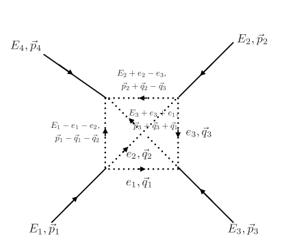
Figure 2: Diagrammatic representation of 4-point function. Note that the particle number is conserved at every vertex.

Note that at every vertex, the particle number is conserved. Assuming that the integral (69) is convergent, the general expression for the 4-point function in the momentum space can be given by

$$<<O_{1}(E_{1},\vec{p}_{1})O_{1}(E_{2},\vec{p}_{2})O_{1}(E_{3},\vec{p}_{3})O_{1}(E_{4},\vec{p}_{4})>>=\int_{\gamma_{1}-i\infty}^{\gamma_{1}+i\infty}\int_{\gamma_{2}-i\infty}^{\gamma_{2}+i\infty}\int_{\gamma_{3}-i\infty}^{\gamma_{3}+i\infty}\prod_{i=1}^{3}\frac{d\alpha_{i}}{2\pi i}\int_{\gamma_{4}-i\infty}^{\gamma_{4}+i\infty}\frac{d\delta}{2\pi i}\rho(\{\alpha_{i}\},\delta)H(\{\alpha_{i}\},\delta)\,.$$ (72)

Here $\gamma_{i}$ and $\rho(\{\alpha_{i}\},\delta)$ are suitable constants and spectral function, respectively.

The integrals (65) and (69) may diverge for certain scaling dimensions. Similar to the 2-point function discussed previously, it needs regularization and renormalization.

References

• [1] C.ย R. Hagen, Scale and conformal transformations in galilean-covariant field theory, Phys. Rev. D 5 (1972) 377โ€“388.
• [2] M.ย Henkel, Schrodinger invariance in strongly anisotropic critical systems, J. Statist. Phys. 75 (1994) 1023โ€“1061, [hep-th/9310081].
• [3] T.ย Mehen, I.ย W. Stewart, and M.ย B. Wise, Conformal invariance for nonrelativistic field theory, Phys. Lett. B 474 (2000) 145โ€“152, [hep-th/9910025].
• [4] Y.ย Nishida and D.ย T. Son, Nonrelativistic conformal field theories, Phys. Rev. D 76 (2007) 086004, [arXiv:0706.3746].
• [5] Y.ย Nishida and D.ย T. Son, An Epsilon expansion for Fermi gas at infinite scattering length, Phys. Rev. Lett. 97 (2006) 050403, [cond-mat/0604500].
• [6] Y.ย Nishida and D.ย T. Son, Fermi gas near unitarity around four and two spatial dimensions, Phys. Rev. A 75 (2007) 063617, [cond-mat/0607835].
• [7] E.ย Braaten and L.ย Platter, Exact Relations for a Strongly Interacting Fermi Gas from the Operator Product Expansion, Phys. Rev. Lett. 100 (2008) 205301, [arXiv:0803.1125].
• [8] S.ย Golkar and D.ย T. Son, Operator Product Expansion and Conservation Laws in Non-Relativistic Conformal Field Theories, JHEP 12 (2014) 063, [arXiv:1408.3629].
• [9] W.ย D. Goldberger, Z.ย U. Khandker, and S.ย Prabhu, OPE convergence in non-relativistic conformal field theories, JHEP 12 (2015) 048, [arXiv:1412.8507].
• [10] R.ย K. Gupta and R.ย Singh, Non-relativistic conformal field theory in the presence of boundary, JHEP 03 (2022) 171, [arXiv:2201.01964].
• [11] R.ย K.ย Gupta and Meenu, Spatially random disorder in unitary fermion system in (4 $-$ $\epsilon$)-dimensions and effective action at finite temperature, JHEP 07 (2023) 003, [arXiv:2210.15998].
• [12] A.ย Bzowski, P.ย McFadden and K.ย Skenderis, Implications of conformal invariance in momentum space, JHEP 03 (2014), 111, [arXiv:1304.7760].
• [13] A.ย Bzowski, P.ย McFadden and K.ย Skenderis, Scalar 3-point functions in CFT: renormalisation, beta functions and anomalies, JHEP 03 (2016), 066, [arXiv:1510.08442].
• [14] A.ย Bzowski, P.ย McFadden and K.ย Skenderis, Conformal $n$-point functions in momentum space, Phys. Rev. Lett. 124 (2020) no.13, 131602, [arXiv:1910.10162].
• [15] D.ย K.ย S, D.ย Mazumdar and S.ย Yadav, $n$-point functions in Conformal Quantum Mechanics: A Momentum Space Odyssey, [arXiv:2402.16947].
• [16] Rajesh Kumar Gupta and Meenu, Work in progress.
• [17] J.ย Ellis, TikZ-Feynman: Feynman diagrams with TikZ, Comput. Phys. Commun. 210 (2017) 103โ€“123, [arXiv:1601.05437].
• [18] B.ย Ananthanarayan, S.ย Bera, S.ย Friot, O.ย Marichev and T.ย Pathak, On the evaluation of the Appell F2 double hypergeometric function, Comput. Phys. Commun. 284 (2023), 108589, [arXiv:2111.05798].