Matrix Completion with Convex Optimization
and Column Subset Selection

Abstract

We introduce a two-step method for the matrix recovery problem. Our approach combines the theoretical foundations of the Column Subset Selection and Low-rank Matrix Completion problems. The proposed method, in each step, solves a convex optimization task. We present two algorithms that implement our Columns Selected Matrix Completion (CSMC) method, each dedicated to a different size problem. We performed a formal analysis of the presented method, in which we formulated the necessary assumptions and the probability of finding a correct solution. In the second part of the paper, we present the results of the experimental work. Numerical experiments verified the correctness and performance of the algorithms. To study the influence of the matrix size, rank, and the proportion of missing elements on the quality of the solution and the computation time, we performed experiments on synthetic data. The presented method was applied to two real-life problems problems: prediction of movie rates in a recommendation system and image inpainting. Our thorough analysis shows that CSMC provides solutions of comparable quality to matrix completion algorithms, which are based on convex optimization. However, CSMC offers notable savings in terms of runtime.

Keywords Matrix completion  $\cdot$ Column Subset Selection  $\cdot$ Low-rank models  $\cdot$ Image inpainting  $\cdot$ Recommendation system  $\cdot$ Nuclear Norm  $\cdot$ Convex Optimization

1 Introduction

Images, time series, graphs, and recommendation systems are just a few examples of data types with natural representation as real-valued matrices. In practice, these matrices often miss entries due to data collection costs, sensor errors, or privacy considerations. To fully exploit the potential of matrix-based datasets, we need to address the missing data problem.

Matrix completion (MC) has found applications in diverse fields such as signal processing, sensor localization, medicine and genomics [1, 2, 3, 4]. Its significance was highlighted in 2006 with the Netflix Prize challenge [5], aimed at improving recommendation systems by predicting unknown ratings. This task involves completing the sparse user-movie rating matrix $\mathbf{M}\in\mathbb{R}^{n_{1}\times n_{2}}$.

Singular Value Decomposition (SVD) is commonly employed to exploit the high correlation in the data,

$$\mathbf{M}=\mathbf{U}\mathbf{\Sigma}\mathbf{V}^{T},$$ (1)

where $\mathbf{U}\in\mathbb{R}^{n_{1}\times n_{1}}$, $\mathbf{V}\in\mathbb{R}^{n_{2}\times n_{2}}$ are orthogonal, and $\mathbf{\Sigma}\in\mathbb{R}^{n_{1}\times n_{2}}$ is non-negative diagonal matrix of singular values, ordered according to their magnitude. Singular values capture the variance in the data. The rank of a matrix is determined by the count of its non-zero singular values. A common approach is to find the matrix with the lowest rank that matches the observed entries. However, directly minimizing the rank is NP-hard [6, 5]. Instead, minimizing the nuclear norm, which is the sum of the singular values of the matrix, is often pursued [7, 8, 9]. Let $\Omega\subseteq\{1,\cdots,n_{1}\}\times\{1,\cdots n_{2}\}$ be the set of indices of the known entries, the convex optimization problem for the exact matrix completion has the form,

$$\left|\begin{aligned} &\mathrm{minimize}&&\|\mathbf{X}\|_{*}\\ &\mathrm{s.t.}&&\mathcal{R}_{\Omega}(\mathbf{X}-\mathbf{M})&=0,\\ \end{aligned}\right.$$ (2)

where $\|\mathbf{X}\|_{*}$ denotes nuclear norm of the decision variable $\mathbf{X}$, $\mathcal{R}_{\Omega}:\mathbb{R}^{n_{1}\times n_{2}}\rightarrow\mathbb{R}^{n_{1}\times n_{2}}$ sets all matrix elements to $0$, except those in the $\Omega$ set, e.g.

$$\mathcal{R}_{\Omega}(\mathbf{X})=\sum_{(i,j)\in\Omega}x_{ij}\mathbf{e}_{i}\mathbf{e}_{j}^{T},$$ (3)

where $\mathbf{e}_{i}$ denotes standard basis vector with $1$ on the $i$-th coordinate and $0$ elsewhere. Nuclear norm minimization is a widely adopted technique for low-rank matrix completion, known for its theoretical guarantees and empirical solid performance [7, 10, 5]. It can be solved in time polynomial time in the matrix dimension, using off-the-shelf Semidefinite Programming (SDP) solvers or tailored first-order methods [6, 10, 5]. However, in large-scale problems, solving these SDP programs, even with first-order methods, can be computationally challenging due to memory requirements [10].

This paper introduces a novel method for the low-rank matrix completion problem, which we call Columns Selected Matrix Completion (CSMC). The CSMC benefits from integrating two fields of modern linear algebra. In particular, it employs the Column Subset Selection (CSS) algorithm to reduce the size of the matrix completion problem. Recovering the most essential columns limits the computational costs of the matrix completion task. In the second stage, the recovered and previously known entries are used to recover $\mathbf{M}$ by solving the standard least squares problem [11, 12, 13]. CSMC is particularly useful when one dimension of $\mathbf{M}$ is much larger than the other, such as in the Netflix Prize scenario. The integration of the two approaches allows CSMC to decrease the computational cost of the convex matrix completion algorithms while maintaining their theoretical guarantees.

1.1 Notation and abbreviations

For a matrix $\mathbf{X}\in\mathbb{R}^{n_{1}\times n_{2}}$ we denote by $\mathbf{x}_{i}$ its $i$-th column, and by $x_{ij}$ its $(i,j)$-th entry. Given the set of column indices $\mathcal{I}\in[n_{2}]$ we use $\mathbf{X}_{:,\mathcal{I}}$ to denote the column submatrix. We consider three types of matrix norms. The spectral norm of $\mathbf{X}$ is denoted by $\|\mathbf{X}\|_{2}$. The Frobenius and the nuclear norm are denoted by $\|\mathbf{X}\|_{F}$ and $\|\mathbf{X}\|_{*}$ respectively. Table 1 contains essential symbols and acronyms.

Notation	Description
$\Omega$	set of indices of the observed entries
$\mathcal{R}_{\Omega}$	sampling operator (3)
$\mathcal{I}$	column indices for the column submatrix $\mathbf{C}$
$\mathbf{X}_{:,\mathcal{I}}$	column submatrix of $\mathbf{X}$ indicated by $\mathcal{I}$
$\mathbf{X}^{\dagger}$	Moore-Penrose inverse of $\mathbf{X}$
$\rho$	percentage of sampled entries
$\alpha$	percentage of sampled columns in the first stage
$r$	rank of $\mathbf{M}$
$\mu_{0}(\mathbf{M})$	the coherence parameter of $\mathbf{M}$
CSS	Column Subset Selection
CSMC	Columns Selected Matrix Completion
CSNN	Columns Selected Nuclear Norm minimization
CSPGD	Columns Selected Proximal Gradient Descent
NN	Nuclear Norm minimization
PGD	Proximal Gradient Descent
MF	Matrix Factorization

Table 1: Notation and abbreviations

1.2 Outline of the paper

The rest of the paper is organized as follows: Section 2 covers related methods, our contribution, and the notations used. In Section 3, we present our method and provide formal analysis, particularly Theorem 3.2, which offers a lower bound on the probability of perfect reconstruction of the matrix, along with conditions on the minimum number of randomly selected columns and the minimum size of the sample of known elements of the reconstructed matrix that ensure achieving this estimate. Section 4 contains experimental results on synthetic and real datasets, confirming the effectiveness of the proposed method.

2 Related work and contribution

2.1 Low-rank matrix completion

The low-rank assumption is grounded in the observation that the real-world datasets inherently possess, or can be effectively approximated by, a low-rank matrix structure [10]. It plays a pivotal role in enhancing the efficiency of algorithms. The algorithms for the low-rank matrix completion typically leverage convex or non-convex optimization in Euclidean spaces [14, 7, 15, 16, 17, 9, 18], or employ Riemannian optimization [19, 20, 21]. The convex methods are the most mature and have strong and well-understood theoretical guarantees. The nuclear norm relaxation draws inspiration from the success of compressed sensing [10, 5, 22, 6] in which $\ell_{1}$ norm minimization is used to recover sparse signal instead of $\ell_{0}$ norm. The matrix rank may be expressed as the $\ell_{0}$ norm of the singular values vector $\mathbf{\sigma}$, while the nuclear norm is defined as its $\ell_{1}$ norm.

Another notable solution, alongside exact matrix completion (2), is presented by Mazumder et al. [15]. To address noisy data and prevent model overfitting, they consider a regularized optimization problem,

$$\underset{\mathbf{X}}{\mathrm{minimize\ }}\frac{1}{2}\|\mathcal{R}_{\Omega}(\mathbf{X})-\mathcal{R}_{\Omega}(\mathbf{M})\|_{F}^{2}+\lambda\|\mathbf{X}\|_{*},$$ (4)

where $\lambda$ is a regularization paramater. The problem (4) benefits from the closed form of the proximal operator for the objective function given by Singular Value Thresholding (SVT) and can be solved with Proximal Gradient descent (PGD) and its modifications [15].

Another class of convex optimization techniques focuses on minimizing the Frobenius norm error for the observed entries while applying constraints on the nuclear norm. It can be solved using the Frank-Wolfe (conditional-gradient descent) algorithm [23]. Despite its low computational cost per iteration, the Frank-Wolfe algorithm exhibits slow convergence rates. Consequently, numerous efforts have been undertaken to develop optimized variants of the algorithm [24, 25].

The non-convex optimization methods aim to minimize least squares error on the observed entries while constraining the rank of the solution with Matrix Factorization (MF) [26, 10],

$$\min_{\mathbf{L}\in\mathbb{R}^{n_{1}\times k},\mathbf{R}\in\mathbb{R}^{n_{2}\times k}}\frac{1}{2}\|\mathcal{R}_{\Omega}(\mathbf{M})-\mathcal{R}_{\Omega}(\mathbf{L}\mathbf{R}^{T})\|^{2}_{F}.$$ (5)

Chen and Chi [10] distinguish three classes of methods solving (5), Alternating Minimization, Gradient Descent and Singular Value Projection. For Alternating Minimization, Jain et al. [14] and Hardt [18] gave provable guarantees. However, these guarantees are worse in terms of coherence, rank and condition number of $\mathbf{M}$.

2.2 Column Subset Selection

Many commonly employed low-rank models, such as Principal Component Analysis (PCA), Singular Value Decomposition (SVD), and Nonnegative Matrix Factorization (NNMF) lack clear interpretability, leading to research on alternatives like CSS and CUR decomposition [27, 28, 29, 30, 31, 32]. CSS provides low-rank representation using the column submatrix of the data matrix $\mathbf{M}\in\mathbb{R}^{n_{1}\times n_{2}}$. Formally, given a matrix $\mathbf{M}\in\mathbb{R}^{n_{1}\times n_{2}}$ and a positive integer $d$, CSS seeks for the column submatrix $\mathbf{C}\in\mathbb{R}^{n_{1}\times d}$ such that

$$\|\mathbf{M}-P_{C}(\mathbf{M})\|_{\xi}$$ (6)

is minimized over all possible $\binom{n_{2}}{d}$ choices for the matrix $\mathbf{C}$. Parameter $\xi\in\{2,F\}$, where $\xi=2$ denotes the spectral and $\xi=F$ the Frobenius norm. Here,

$$P_{C}=\mathbf{C}\mathbf{C}^{\dagger},$$ (7)

is the projection onto the $d$-dimensional space spanned by the columns $\mathbf{C}$ and $\mathbf{C}^{\dagger}$ denotes the Moore-Penrose pseudoinverse [33]. On the other hand, CUR decomposition explicitly selects a subset of columns and rows from the original matrix to construct the factorization [30, 29].

Extensive research focuses on fully-observed matrices, which may not be practical for real-world applications [27, 28, 29, 30, 31, 32]. Bridging the research gap between CSS, CUR and matrix completion is a recently recognized challenge [34, 35, 36, 37]. In this context, two important questions emerge. The first one is about selecting meaningful columns (or rows) from partially observed data and applying CSS and CUR in matrix completion algorithms. Our method benefits from the fact that under standard assumptions about matrix incoherence, a high-quality column subset can be obtained by randomly sampling each column [38]. However, in the case of the coherent matrices, Wang and Singh [34] propose active sampling to dynamically adjust column selection during the sampling process, albeit with increased computational complexity.

The application of CUR and CSS in MC tasks typically involves altering the sampling scheme to relax assumptions about the matrix or reduce sample complexity [36, 37, 35]. However, estimating leverage scores, a key requirement in these methods, poses a significant challenge [34].

Cai et al. [3] showcase the potential of CUR in low-rank matrix completion, introducing a novel sampling strategy called Cross-Concentrating Sampling (CCS) and a fast non-convex Iterative CUR Completion (ICURC) algorithm. However, CCS requires $\mathcal{O}(r^{2}n\ln^{2}(n))$ observed entries, where $n=\max\{n_{1},n_{2}\}$, which is a factor of $r$ worse than the nuclear norm minimization-based approach. The optimization problem solved by ICURC imposes constraints on the rank of the matrix, thus introducing an additional parameter that requires tuning.

Our approach is closely related to the work of Xu et al., who presented CUR++, an algorithm for partially observed matrices [38]. It computes a low-rank approximation of the matrix based on randomly selected columns and rows, along with a subset of observed entries. The authors formulate a least squares optimization problem for matrix recovery based on fully observed columns and rows, and provide a theoretical analysis of the problem. However, the reconstruction procedure requires finding eigenvectors of the observed submatrices, which adds a computational burden.

2.3 Our contributions

This paper addresses the challenge of completing rectangular matrices by integrating principles from Column Subset Selection and Low-rank Matrix Completion. Our approach involves solving convex optimization problems. Our main contributions are as follows:

1. We introduce a two-staged matrix completion method, CSMC, dedicated to recovering rectangular matrices with one direction significantly larger than the other ($n_{1}<<n_{2}$).

2. We offer a formal analysis, including Theorem 3.2, which establishes a lower bound on the probability of achieving perfect matrix reconstruction in the second stage of CSMC. This theorem contains necessary conditions regarding the minimum number of randomly selected columns ($d=\mathcal{O}(r\ln{r})$) and the minimum sample size of known elements ($|\Omega|=\mathcal{O}(n_{2}r\ln{(n_{2}r)})$) required for accurate reconstruction of an incoherent matrix of rank $r$.

3. We develop two algorithms dedicated to problems of different sizes: Columns Selected Nuclear Norm (CSNN) and Columns Selected Proximal Gradient Descent (CSPGD).

4. We present results of several numerical experiments on synthetic and real-world datasets to verify theoretical results. The performance of the presented algorithms is compared with commonly used matrix completion algorithms described in the literature. Additionally, we apply the CSMC method to two real-life scenarios: movie recommendation and image inpainting.

3 Columns Selected Matrix Completion (CSMC) method overview

In the CSMC, the completion of the matrix $\mathbf{M}\in\mathbb{R}^{n_{1}\times n_{2}}$ is divided into two stages. In the first stage, CSMC selects the subset of $d$ columns and fills it with an established matrix completion algorithm. In the second stage, the least squares problem is solved. Each of the presented variants of the CSMC methods adopts the following procedure (Fig. 1).

Stage I: Sample and fill

CSMC selects $d$ columns of $\mathbf{M}\in\mathbb{R}^{n_{1}\times n_{2}}$ according to the uniform distribution over the set of all indices. Let $I\subseteq\{1,\cdots,n_{2}\}$ denote the set of the indices of the selected columns. The submatrix formed by selected columns, $\mathbf{C}:=\mathbf{M}_{:I}$, $\mathbf{C}\in\mathbb{R}^{n_{1}\times d}$ is recovered using the chosen matrix completion algorithm.

Stage II: Solve least squares

Let $\mathbf{\hat{C}}\in\mathbb{R}^{n_{1}\times d}$ be the output of the Stage I. The CSMC solves the following convex optimization problem,

$$\min\limits_{\mathbf{Z}\in\mathbb{R}^{d\times n_{2}}}\frac{1}{2}\|\mathcal{R}_{\Omega}(\mathbf{M})-\mathcal{R}_{\Omega}(\mathbf{\hat{C}}\mathbf{Z})\|_{F}^{2},$$ (8)

where $\mathcal{R}_{\Omega}:\mathbb{R}^{n_{1}\times n_{2}}\rightarrow\mathbb{R}^{n_{1}\times n_{2}}$ is the sampling operator (eq. 3). Let $\mathbf{\hat{Z}}\in\mathbb{R}^{d\times n_{2}}$ be a solution to the problem (8). The CSMC output with the matrix $\mathbf{\hat{M}}=\mathbf{\hat{C}}\mathbf{\hat{Z}}$.

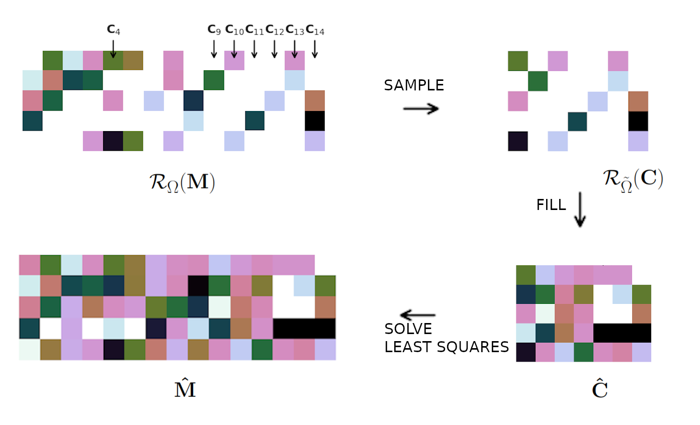
Figure 1: The CSMC method overview.

Algorithm 1 CSMC-$\alpha$

Require: $\mathcal{R}_{\Omega}(\mathbf{M})$: $n_{1}\times n_{2}$-matrix

Require: $\alpha$: Ratio of the selected columns

$I\leftarrow\text{Uniformly sample }\alpha\cdot n_{2}$ indices

$\mathbf{C}_{\text{missing}}\leftarrow\mathcal{R}_{\Omega}(\mathbf{M})_{:I}$

$\mathbf{\hat{C}}\leftarrow\text{MC}(\mathbf{C}_{\text{missing}})$ $\triangleright$ Complete submatrix $\mathbf{C}\in\mathbb{R}^{n_{1}\times d}$.

$\mathbf{\hat{Z}}\leftarrow\text{arg}\min\limits_{\mathbf{Z}\in\mathbb{R}^{n_{2}}}\frac{1}{2}\|\mathcal{R}_{\Omega}(\mathbf{M})-\mathcal{R}_{\Omega}(\mathbf{\hat{C}}\mathbf{Z})\|_{F}^{2}$

$\mathbf{\hat{M}}\leftarrow\mathbf{\hat{C}}\mathbf{\hat{Z}}$

return $\mathbf{\hat{M}}$

3.1 Theoretical results

In their seminal work, Candes and Recht proved that, under certain assumptions, solving nuclear norm minimization leads to successful matrix recovery [17]. There has been a significant amount of research extending these results to noisy settings, improved bounds on the sample complexity and analyzing the robustness of the nuclear norm minimization algorithms to noise and outliers [8, 7, 9, 5]. Recht [7] greatly simplified the analysis and provided a foundation for understanding the potential and limitations of the method in practical matrix completion scenarios. The theoretical guarantees rely on properties such as matrix rank, number and distribution of observed entries and the fact that the singular vectors of the matrix are uncorrelated with the standard basis. The last property is formalized with the matrix coherence and defined as follows [17].

Definition 3.1.

Let $U$ be a subspace of $\mathbb{R}^{n}$ of dimension $r_{U}$ and $P_{U}$ be the orthogonal projection onto $U$. The coherence parameter of $U$ is defined as

$$\mu(U)=\frac{n}{r_{U}}\max_{1\leq i\leq n}||P_{U}\mathbf{e}_{i}||_{2}^{2},$$ (9)

where $\mathbf{e}_{i}$ for $i=1,\ldots n$ are the standard basis vectors of $\mathbb{R}^{n}$.

The coherence parameter of the rank-$\tilde{r}$ matrix $\mathbf{X}$ is given by $\mu_{0}(\mathbf{X})=\max\{\mu(U),\mu(V)\}$ where $U$ and $V$ are the linear spaces spanned by its $\tilde{r}$ left and right singular vectors respectively.

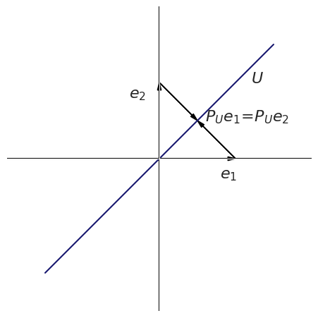
(a) $\mu(U)=1$.

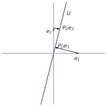
(b) $1<\mu(U)<2$

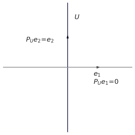
(c) $\mu(U)=2$

Figure 2: Coherence of the one-dimensional subspace $U\subset\mathbb{R}^{2}$. 2(a) depicts $U$ spanned by $(\frac{1}{\sqrt{2}},\frac{1}{\sqrt{2}})$ with the smallest coherence $\mu(U)=1$, while 2(c) presents $U$ spanned by one of the standard basis vectors $\mathbf{e}_{2}$ which achieves maximal coherence $\mu(U)=2$

We assume that observed entries are sampled uniformly at random. We begin with a discussion on how the crucial characteristics of the matrix $\mathbf{M}$ completion problem are transferred to the task of filling in the submatrix $\mathbf{C}$. Since $\mathbf{C}$ consists of randomly selected $d$ columns of $\mathbf{M}$, the rank of $\mathbf{C}$ is bounded by a minimum of $r$ and $d$, and the entries of $\mathbf{C}$ also follow a uniform distribution. The following theorem demonstrates that for an incoherent, well-conditioned matrix $\mathbf{M}$, if the submatrix $\mathbf{C}$ is composed of $\mathcal{O}(r\ln(rn_{2}))$ sampled columns, it will exhibit low coherence.

Theorem 3.1 (Corollary 3.6 in Cai et al. [39]).

Suppose that $\mathbf{M}\in\mathbb{R}^{n_{1}\times n_{2}}$ has rank $r$ and coherence bounded by $\mu_{0}(\mathbf{M})$. Suppose that $I\ \subseteq\{1,\ldots n_{2}\}$ is chosen by sampling uniformly without replacement to yield $\mathbf{C}=\mathbf{M}_{:I}$. Let $d$ be the number of sampled columns such that $d\geq 1.06\mu_{0}(\mathbf{M})r\ln(rn_{2})$. Then

$$\mu_{0}(\mathbf{C})\leq 100\kappa^{2}({\mathbf{M}})\mu_{0}({\mathbf{M}}),$$ (10)

with a probability at least $1-\frac{1}{n_{2}}$, where $\kappa(\mathbf{M})$ denotes the spectral condition number of $\mathbf{M}$, given by $\kappa(\mathbf{M}):=\|\mathbf{M}\|_{2}\|\mathbf{M}^{\dagger}\|_{2}$.

In this section, the primary focus lies on assessing the recovery capabilities of the least-squares problem during the second stage of the CSMC. In particular, we assume that submatrix $\mathbf{C}$ is fully observed or perfectly recovered and provide assumptions that solving

$$\min_{\mathbf{Z}\in\mathbb{R}^{d\times n_{2}}}\frac{1}{2}\|\mathcal{R}_{\Omega}(\mathbf{M})-\mathcal{R}_{\Omega}(\mathbf{C}\mathbf{Z})\|_{F}^{2}$$ (11)

will output $\mathbf{\hat{Z}}\in\mathbb{R}^{d\times n_{2}}$, such that $\mathbf{M}=\mathbf{C}\mathbf{\hat{Z}}$ holds with high probability. The following analysis is guided by the analysis of the CUR+ in the work of Xu et al. [38]. However, in contrast to CUR+, solving (11) does not require computing singular vectors of $\mathbf{C}$. The main result of this section is given by the Theorem 3.2. We believe that the following main result broadens the result of Xu et al. formulated as Theorem 2 in [38]. The proof of Theorem 3.2 is provided in the appendix.

Theorem 3.2.

Let $r$ be the rank of $\mathbf{M}\in\mathbb{R}^{n_{1}\times n_{2}}$ and let $\mathbf{C}\in\mathbb{R}^{n_{1}\times d}$ be a column submatrix of $\mathbf{M}$ formed by uniformly sampled without replacement $d$ columns. Let $\tilde{r}$ denote the rank of $\mathbf{C}$. Assume that for the parameter $\gamma>0$,

1. $d\geq 7\mu_{0}(\mathbf{M})r(\gamma+\ln r)$,

2. $|\Omega|\geq\tilde{r}n_{2}\mu_{0}(\mathbf{C})\left(\gamma+\ln{(\frac{n_{2}\tilde{r}}{2})}\right)$.

Let $\mathbf{\hat{Z}}\in\mathbb{R}^{d\times n_{2}}$ be the minimizer of the problem 11. Then, with a probability at least $1-3e^{-\gamma}$, we have $\mathbf{M}=\mathbf{C}\mathbf{\hat{Z}}$.

3.2 Implementation

The CSMC is a versatile method for solving matrix completion problems. It allows the incorporation of various matrix completion algorithms in the first step and least squares algorithms in the second step. This paper discusses two algorithms that implement the CSMC method, each tailored to address matrix completion problems of different sizes.

1. Columns Selected Nuclear Norm (CSNN) in which submatrix is filled with the exact nuclear norm minimization using SDP solver. The CSNN is dedicated to recovering the small and medium size $\mathbf{M}$. We found the first-order Splitting Conic Solver (SCS) as an efficient way to solve the SDP [40] in the Stage I. To find the optimum of the regression problem (8), we directly solve the least squares for the observed entries in each column. This approach is simple and allows to create fairly efficient distributed implementations.

2. Columns Selected Proximal Gradient Descent (CSPGD) in which inexact nuclear norm minimization (4) is solved by Proximal Gradient Descent (PGD). PGD is an efficient first-order method for convex optimization. It leverages the closed formula for the proximal operator for the objective function (4) and allows completing large matrices [15]. To find the optimum of the regression problem (8), we directly solve the least squares for the observed entries in each column.

We have developed and released open-source code implementing both the CSNN minimization algorithm and CSPGD methods. These algorithms support both Numpy arrays [41] and PyTorch tensors [42], with the latter offering the advantage of GPU acceleration for faster computation. The semidefinite programming is solved using the Splitting Conic Solver (SCS) [43]. The code is written in Python 3.10 and is available at https://github.com/ZAL-NASK/CSMC.

4 Numerical experiments

All testing examples were implemented in Python 3.10. For benchmarking purposes, the Matrix Factorization (MF) and Iterative SVD algorithms were utilized from the fancyimpute library [44].

4.1 Synthetic data set

To evaluate the proposed CSMC method, we compared the performance of the Columns Selected Nuclear Norm algorithm with the exact Nuclear Norm (NN) minimization in a controlled setting. The goal of each experiment was to recover a random $300\times 1000$ matrix $\mathbf{M}$ with the ratio of missing entries $\rho$. To control the rank of $\mathbf{M}$ equal to $r$, the test matrix was generated as a product of the $n_{1}\times r$ matrix $\mathbf{A}$ and $r\times n_{2}$ matrix $\mathbf{B}$. Matrices $\mathbf{A}$ and $\mathbf{B}$ were generated in two steps. In the first one, matrix entries were sampled from the normal distribution $\mathcal{N}(0,1)$. In the second step, noise matrices with the ratio $0.3$ of non-zero entries were added to each matrix.

Experiment S I

To assess the sample complexity of the presented methods, we varied the ratio of known entries $\rho$ and the number of sampled columns $d$. Every setup was executed over $N_{\text{trial}}=20$ independent trial runs. The performance of the algorithms NN and CSNN-${\alpha}$, $\alpha=\{0.1,\cdots,0.9\}$ was evaluated over all trials. To inquire how many columns should be sampled to achieve a satisfying algorithm relative error,

$$\epsilon:=\frac{\|\mathbf{M}-\mathbf{\mathbf{\hat{M}}}\|_{F}}{\|\mathbf{M}\|_{F}},$$ (12)

we calculated an empirical cumulative distribution function (ECDF) to display the proportion of trials achieved given approximation error [45, 46]. ECDF is defined as $\hat{F}_{S}:\mathbb{R}_{+}\rightarrow[0,1]$,

$$\hat{F}_{S}(a)=\frac{|\{s|\epsilon_{s}\leq a\}|}{|S|},$$ (13)

where each trial is represented as $s$, $\epsilon_{s}$ denotes the relative error reached by the solution of $s$, and $S$ denotes the set of all trials for the given parameters setup. We also compared the analyzed algorithms’ runtime (in seconds). Since CSMC methods consist of two stages, while other algorithms are one staged, we did not compare iteration numbers of algorithms to achieve solutions of prescribed quality.

Experiment S II

With the same experiment settings we benchmarked CSNN-$\alpha$ for $\alpha\in\{0.1,\cdots,0.5\}$ algorithm, Matrix Factorization (MF) [47, 26], Iterative SVD [48], and Nuclear Norm minimization (NN).

Results

Experiments were executed on the Linux workstation equipped with 11th Gen Intel(R) Core(TM) i7-1165G7 @ 2.80GHz (8 cores) and 32GB RAM.

Fig. 3 shows that sampling CSNN-$0.2$ offered a tenfold (10x) increase in time savings compared to the NN algorithm and maintains a solution quality. Although MF was faster than CSNN-$\alpha$ algorithms (Fig. 5), the magnitude of the relative error for CSNN-$0.3$ and CSNN-$0.5$ was significantly smaller for rank-5 and rank-10 cases, respectively. In that case, both algorithms returned a solution of superior quality (Fig. 4).

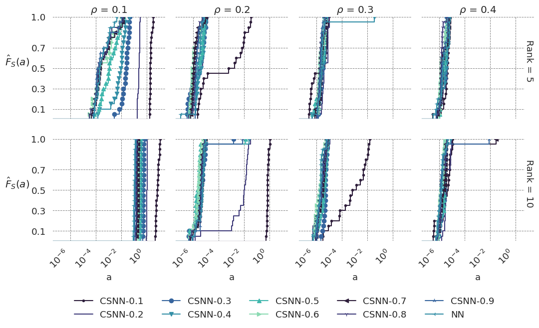
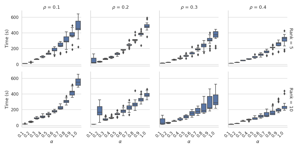
Figure 3: Results S I: ECDF (13) and runtimes depending on the matrix rank and rate of the known entries for NN and CSNN-$\alpha$, $\alpha\in\{0.1,\cdots,0.9\}$, $\mathbf{M}\in\mathbb{R}^{300\times 1000}$. Sampling with CSNN-$0.2$ resulted in a tenfold (10x) improvement in time efficiency over the NN algorithm while preserving solution quality.

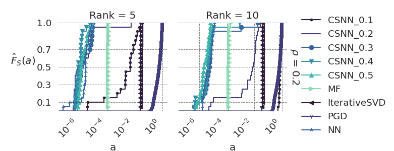
Figure 4: Results S II: ECDF (13) curves depending on the matrix rank and rate of the known entries for NN and CSNN-$\alpha$, $\alpha\in\{0.1,\cdots,0.9\}$, $\mathbf{M}\in\mathbb{R}^{300\times 1000}$. The relative error magnitude for CSNN-$0.3$ and CSNN-$0.5$ was notably lower in rank-5 and rank-10 scenarios, respectively, compared to MF.

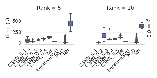
Figure 5: Results S II: ECDF (13) curves depending on the matrix rank and rate of the known entries for NN and CSNN-$\alpha$, $\alpha\in\{0.1,\cdots,0.9\}$, $\mathbf{M}\in\mathbb{R}^{300\times 1000}$.

4.2 Recommendation system

Here, we assessed the performance of CSNN and CSPGD algorithms within the context of the Netflix Prize scenario, where matrix completion was employed as a rating prediction technique. Data sets used for the benchmarking are publicly available data sets from the Movielens research project [49].

Settings

To benchmark CSNN and CSPGD algorithms, we constructed two data sets: Movie Lens Small and Movie Lens Big. The Movie Lens Small was represented by $\mathbf{M}\in\mathbb{R}^{140\times 668}$ matrix obtained from the Movie Lens Small dataset, which contained 100 000 5-star ratings applied to 9742 movies by 610 users. Since the original matrix was too large for SDP solvers, we followed the procedure described in [3] to obtain a submatrix of the desired size. Specifically, we sorted the data by user frequency rate and took data containing rates made by the top 60% users. Then, we sorted the obtained data by movie frequency rate and selected the top 50% movies. The obtained matrix had $\rho=0.25$ known entries. We evaluate CSPGD algorithms on the Movielens 25M data set, containing 25 million ratings applied to 62,000 movies by 162,000 users. Again, due to the large size and low observation rate, we extracted a $654\times 27813$ matrix $\mathbf{M}$. The known entries rate $\rho$ was equal to 0.09.

We assessed the performance of the NN and CSNN-$\alpha$ for $\alpha\in\{0.3,0.4,0.5,0.7\}$ and CSPGD-$\alpha$ for $\alpha\in\{0.3,0.5\}$. We followed previous work [3] and employed the Cross-Validation method. In each trial of the experiment, $\Omega$ set was randomly split into training and testing sets denoted by $\Omega_{\text{train}}$ and $\Omega_{\text{test}}$ [50]. Specifically, we randomly selected $\rho$ rate of the observed set, and by assigning the null values to the rest of the entries, we constructed $\mathcal{R}_{\Omega_{\text{train}}}(\mathbf{M})$ matrix. We evaluated each algorithm on the $\Omega_{\text{test}}$ set. We conducted 20 independent experimental trials under each scenario.

We compared Normalized Mean Absolute Error (NMAE) calculated as

$$\text{NMAE}=\frac{1}{|\Omega_{\text{test}}|(m_{\text{max}}-m_{\text{min}})}\sum_{(i,j)\in\Omega_{\text{test}}}|\mathbf{\hat{M}}-\mathbf{M}|,$$ (14)

where $m_{\text{max}}$ and $m_{\text{min}}$ denote the maximum and minimum rating, respectively, and $\Omega_{\text{test}}$ denotes the set of indices in test set. This metric is widely used to assess collaborative filtering tasks [3]. The quality of the recommendation was also measured as hit-rate, defined as

$$\text{HR}=\frac{\#hits}{|\Omega_{\text{test}}|},$$ (15)

where a predicted rating was considered a hit if its rounded value equals the actual rating in the test set [3].

Results

Fig. 6 shows that the predictions of CSNN-$0.7$ maintained the quality of the NN algorithm in terms of NMAE: (0.16 vs 0.13) and HR (0.23 vs 0.25), and results in runtime savings from 57 seconds to 40 seconds (Table 2). CSPGD algorithms were much faster than PGD (Fig. 7). The HR values for PGD and CSPGD-$0.3$ were equal to 0.28 and 0.24, respectively (Table 3).

	NMAE		HR		Time [s]
	mean	std	mean	std	mean	std
Algorithm
CSNN-0.3	0.271	0.028	0.172	0.005	10.137	1.118
CSNN-0.4	0.240	0.060	0.191	0.005	17.677	2.005
CSNN-0.5	0.248	0.176	0.208	0.006	28.673	2.419
CSNN-0.7	0.156	0.011	0.232	0.004	39.893	8.595
NN	0.127	0.001	0.255	0.006	56.924	2.435

Table 2: Results on Movie Lens Small dataset; NN and CSNN-$\alpha$ algorithms, $\alpha\in\{0.3,0.4,0.5,0.7\}$.

Figure 6: Results on Movie Lens Small dataset; NN and CSNN-$\alpha$ algorithms, $\alpha\in\{0.3,0.4,0.5,0.7\}$.

	NMAE		HR		Time [s]
	mean	std	mean	std	mean	std
Algorithm
CSPGD-0.3	0.138	0.001	0.245	0.002	23.032	0.321
CSPGD-0.5	0.135	0.001	0.252	0.001	27.774	0.299
PGD	0.119	0.001	0.281	0.001	449.026	9.502

Table 3: Results on Movie Lens Big dataset; PGD and CSPGD-$\alpha$ algorithms for $\alpha\in\{0.3,0.5\}$.

Figure 7: Results on Movie Lens Big dataset; PGD and CSPGD-$\alpha$ algorithms for $\alpha\in\{0.3,0.5\}$.

4.3 Image recovery

Image inpainting, a technique in image processing and computer vision, fills in missing or corrupted parts. Additionally, estimating random missing pixels can be treated as a denoising method or utilized to accelerate rendering processes. Low-rank models are highly effective for this task, leveraging the assumption that images typically exhibit low-rank structures. The primary information of the image matrix is dominated by its largest singular values while setting the smallest singular values to zero can be done without losing essential details.

Settings

The data set contained ten grey-scaled pictures of bridges downloaded from the public repository . Images were represented as $240\times 360$ matrices. We assessed the performance of the algorithms among 100 independent trials (ten trials per picture). The quality of the reconstructed image was assessed with the signal-to-noise ratio (SNR)

$$\text{SNR}(\mathbf{\hat{M}})=20\log_{10}\left(\frac{\|\mathbf{M}\|_{F}}{\|\mathbf{\hat{M}}-\mathbf{M}\|_{F}}\right)$$ (16)

and the relative error (12).

Results

The CSNN-$0.7$ solutions maintained the quality of the NN in terms of SNR (Table 4). As shown in Fig. 9, CSNN-$0.5$ offered considerable time savings and good relative error. Fig. 8 presents one of the completed pictures.

Bridge with $\rho=20\%$ known entries

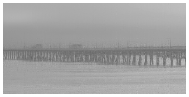
Bridge restored with CSNN-0.5

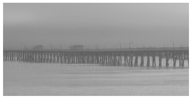
Bridge restored with CSNN-0.7

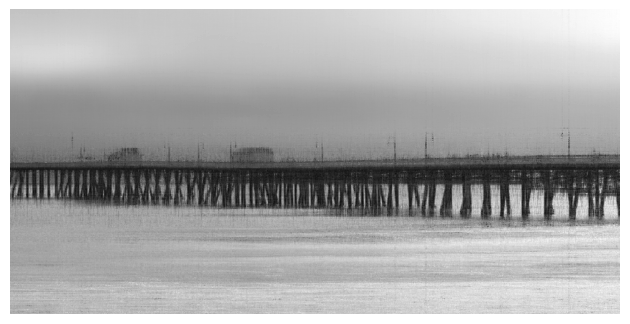
Bridge restored with NN

Figure 8: Image inpainting; NN and CSNN algorithms, $\rho=20\%$ known entries.

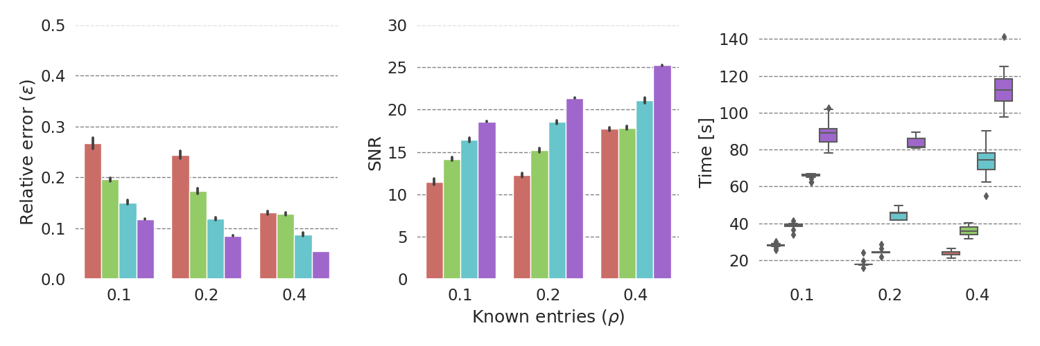
Figure 9: Results for image inpainting; NN and CSNN-$\alpha$ algorithms for $\alpha\in\{0.3,0.4,0.5,0.7\}$.

	SNR			Relative error ($\epsilon$)			Time [s]
Known entries ratio $\rho$	0.4	0.2	0.1	0.4	0.2	0.1	0.4	0.2	0.1
Algorithm
CSNN_0.3	18.844	10.829	7.366	0.114	0.289	0.438	16.306	12.026	19.365
CSNN_0.4	17.708	12.245	11.491	0.130	0.245	0.268	24.151	17.997	28.123
CSNN_0.5	17.851	15.245	14.172	0.128	0.173	0.196	35.719	24.424	38.647
CSNN_0.7	21.134	18.526	16.458	0.088	0.119	0.151	73.670	44.948	65.639
NN	25.221	21.377	18.582	0.055	0.085	0.118	113.215	83.196	88.966

Table 4: Results for image inpainting; NN and CSNN-$\alpha$, $\alpha\in\{0.3,0.4,0.5,0.7\}$.

5 Conclusion

This paper introduces the Columns Selected Matrix Completion (CSMC) method, devised to enhance the time efficiency of nuclear norm minimization algorithms for low-rank matrix completion tasks. Through a two-staged approach, CSMC strategically applies a low-rank matrix completion algorithm to a reduced problem size in the first stage, followed by the minimization of least squares error in the second stage. Theoretical analysis provides provable guarantees for CSMC, demonstrating its efficacy in perfectly recovering the matrix under standard assumptions.

Numerical simulations confirm the theoretical findings, showcasing CSMC’s ability to achieve significant time savings while preserving solution quality compared to nuclear norm minimization algorithms. Moreover, comparisons with alternative methods underscore CSMC’s competitive performance in terms of relative approximation error.

The presented CSMC methods sample columns following a uniform distribution and employ nuclear norm-based matrix completion algorithms. Nevertheless, the framework presented exhibits versatility, accommodating alternative sampling methods and matrix completion techniques. Recent studies have introduced adaptive sampling strategies [36, 34]. The application of such methodologies could effectively address matrices with higher coherence or reduce sample complexity, which we intend to explore in forthcoming research.

Appendix A Proof of Theorem 3.2 and supporting theorems

We present a comprehensive proof of Theorem 3.2, accompanied by the development of two additional theorems, namely A.2 and A.4, which are our original contributions. The proofs for these supplementary theorems are provided within this work. Additionally, the cited theorems from the literature have their proofs outlined therein.

We assume that $\mathbf{C}\in\mathbb{R}^{n_{1}\times d}$ is a column submatrix of $\mathbf{M}\in\mathbb{R}^{n_{1}\times n_{2}}$. $\mathbf{C}$ is obtained by sampling uniformly without replacement $d$ columns of $\mathbf{M}$. Let $r$ be the rank of $\mathbf{M}$ and let $\tilde{r}$ be the rank of $\mathbf{C}$. We assume that the compact SVD of $\mathbf{C}$ is given by,

$$\mathbf{C}=\mathbf{\tilde{U}}\mathbf{\tilde{\Sigma}}\mathbf{\tilde{V}^{T}},$$ (17)

where $\mathbf{\tilde{U}}\in\mathbb{R}^{n_{1}\times\tilde{r}}$, $\mathbf{\tilde{V}}\in\mathbb{R}^{n_{2}\times\tilde{r}}$, and $\mathbf{\tilde{\Sigma}}\in\mathbb{R}^{\tilde{r}\times\tilde{r}}$.

We denote as $\mu_{0}(\mathbf{M})$ and $\mu_{0}(\mathbf{C})$ the coherence parameters of $\mathbf{M}$ and $\mathbf{C}$.

We denote as $\tilde{U}$ the subspace spanned by the first $\tilde{r}$ left singular vectors of $\mathbf{C}$. The orthogonal projection onto $\tilde{U}$ is given by

$$P_{\tilde{U}}=\mathbf{\tilde{U}}\mathbf{\tilde{U}}^{T}.$$ (18)

The following lemma can be found in [38] and shows that under the incoherence assumption, uniform sampling outputs a high-quality solution to the CSS problem, with high quality.

Theorem A.1 (Theorem 9 in Xu et al. [38]).

Let $\tilde{U}_{\psi}$ denote subspace spanned by the $\psi$ first left singular vectors of $\mathbf{C}$ and let $P_{\tilde{U}_{\psi}}$ denote orthogonal projection on $\tilde{U}_{\psi}$. Then for parameter $\gamma>0$, with probability $1-2e^{-\gamma}$ we have

$$\|\mathbf{M}-P_{\tilde{U}_{\psi}}\mathbf{M}\|_{2}^{2}\leq\sigma_{\psi+1}^{2}\left(1+\frac{2n_{2}}{d}\right),$$ (19)

if $d\geq 7\mu(U_{\psi})\psi(\gamma+\ln{\psi})$, where $d$ denotes number of sampled columns in $\mathbf{C}$, $\sigma_{\psi+1}$ is the $(\psi+1)$-th largest singular value of $\mathbf{M}$ and $\mu(U_{\psi})$ is the coherence of the subspace spanned by $\psi$ first left singular vectors of $\mathbf{M}$,

The following remark is the immediate consequence of the Theorem A.1.

Remark A.1.

Let $\psi\geq r$, where $r$ is the rank of $\mathbf{M}$. Then $\sigma_{\psi+1}=\sigma_{r+1}=0$ and with probability $1-2e^{-\gamma}$,

$$\|\mathbf{M}-P_{\tilde{U}}\mathbf{M}\|^{2}_{2}=0,$$ (20)

provided that $d\geq 7\mu_{0}(\mathbf{M})r(\gamma+\ln{r})$.

We now bound the distance measured in the spectral norm between $\mathbf{M}$ and $\mathbf{\hat{M}}=\mathbf{C}\mathbf{\hat{Z}}$. To do that, we assume that the objective function $g:\mathbb{R}^{\tilde{r}\times n_{2}}\rightarrow\mathbb{R}$,

$$g(\mathbf{Y})=\frac{1}{2}\|\mathcal{R}_{\Omega}(\mathbf{M})-\mathcal{R}_{\Omega}(\mathbf{\tilde{U}}\mathbf{Y})\|_{F}^{2}$$ (21)

is strongly convex [51], where the strong convexity is defined as follows.

Definition A.1 (Boyd and Vandenberghe [51]).

A function $g:\mathbb{R}^{\tilde{r}\times n_{2}}\rightarrow\mathbb{R}$ is strongly convex with parameter $\beta>0$ if $h(\mathbf{X})=g(\mathbf{X})-\frac{\beta}{2}\|\mathbf{X}\|_{F}^{2}$ is convex.

The following remarks provide a helpful characterization of strongly convex functions.

Remark A.2 (Boyd and Vandenberghe [51]).

A function $g:\mathbb{R}^{\tilde{r}\times n_{2}}\rightarrow\mathbb{R}$ is strongly convex with parameter $\beta>0$ if $g$ is everywhere differentiable and

$$g(\mathbf{Y})\geq g(\mathbf{X})+\langle\nabla g(\mathbf{X}),\mathbf{Y}-\mathbf{X}\rangle+\frac{\beta}{2}\|\mathbf{Y}-\mathbf{X}\|_{F}^{2},$$ (22)

for any $\mathbf{X},\mathbf{Y}\in\mathbb{R}^{\tilde{r}\times n_{2}}$, where inner product is defined as

$$\langle\mathbf{X},\mathbf{Y}\rangle=\text{tr}(\mathbf{X}^{T}\mathbf{Y}).$$ (23)

Remark A.3 (Boyd and Vandenberghe [51]).

If $g$ is twice differentiable, then $g(\mathbf{X})$ is strongly convex with parameter $\beta>0$ if $\nabla^{2}g(\mathbf{X})\succeq\beta\mathbf{I}$ for any $\mathbf{X}\in\mathbb{R}^{\tilde{r}\times n_{2}}$.

We now provide the formula for the first-order and the second-order partial derivatives of $g$. Let $y_{sw}$ denote the $(s,w)$ entry of the matrix $\mathbf{Y}$, and $m_{lw}$ denote $(l,w)$ entry of $\mathbf{M}$ then the partial derivative of $g$ with respect to $y_{sw}$ is given by following formula,

$$\frac{\partial g}{\partial y_{sw}}=-\sum\limits_{l:(l,w)\in\Omega}(m_{lw}-\sum_{i=1}^{\tilde{r}}{\tilde{u}_{li}}y_{iw})\tilde{u}_{ls}=\sum\limits_{l:(l,w)\in\Omega}(\sum_{i=1}^{\tilde{r}}{\tilde{u}_{li}}y_{iw}-m_{lw})\tilde{u}_{ls}.$$ (24)

The second-order partial derivative with respect to $y_{pq}$ and $y_{sw}$ is equal to

$$\frac{\partial^{2}g}{\partial y_{sw}\partial y_{pq}}=\begin{cases}\sum\limits_{l:(l,w)\in\Omega}\tilde{u}_{ls}\tilde{u}_{lp}&w=q,\\ 0&w\neq q.\end{cases}$$ (25)

The following theorem shows that under certain assumptions, $\mathbf{\hat{M}}=\mathbf{C}\mathbf{\hat{Z}}$ is close to the matrix $\mathbf{M}$ in the spectral norm. Those assumptions include that i) $P_{\tilde{U}}\mathbf{M}$ is close to $\mathbf{M}$, ii) $g$ is strongly convex with parameter $\beta$. The following proofs take inspiration from the work of Xu et al. [38].

Theorem A.2.

Suppose that $\|\mathbf{M}-P_{\tilde{U}}\mathbf{M}\|_{2}^{2}\leq\Delta$ for the parameter $\Delta>0$, and let $\tilde{U}$ be the subspace of $\mathbb{R}^{n_{1}}$ spanned by the first $\tilde{r}$ left singular vectors of $\mathbf{C}$, $P_{\tilde{U}}=\mathbf{\tilde{U}}\mathbf{\tilde{U}^{T}}$. Assume that $g$ is strongly convex with a parameter $\beta$, then

$$\|\mathbf{M}-\mathbf{\hat{M}}\|_{2}^{2}\leq\Delta+\frac{2n_{1}\tilde{r}\Delta}{\beta}.$$ (26)

Proof.

Set $\mathbf{Y}_{1}=\mathbf{\mathbf{\tilde{U}}^{T}}\mathbf{M}$ , then from the assumptions

$$\|\mathbf{M}-\mathbf{\tilde{U}}\mathbf{Y}_{1}\|_{2}^{2}\leq\Delta.$$ (27)

Thus

$$\frac{1}{r^{\prime}}\|\mathbf{M}-\mathbf{\tilde{U}}\mathbf{Y}_{1}\|_{F}^{2}\leq\|\mathbf{M}-\mathbf{\tilde{U}}\mathbf{Y}_{1}\|_{2}^{2}\leq\Delta,$$ (28)

where $r^{\prime}$ denotes the rank of the matrix $(\mathbf{M}-\mathbf{\tilde{U}}\mathbf{Y}_{1})\in\mathbb{R}^{n_{1}\times n_{2}}$ and

$$\|\mathcal{R}_{\Omega}(\mathbf{M})-\mathcal{R}_{\Omega}(\mathbf{\tilde{U}}\mathbf{Y}_{1})\|_{F}^{2}\leq\|\mathbf{M}-\mathbf{\tilde{U}}\mathbf{Y}_{1}\|_{2}^{2}\leq r^{\prime}\Delta.$$ (29)

Since any of the matrix dimensions bounds rank, $r^{\prime}\leq n_{1}$ (for thick matrices $n_{1}<n_{2}$)

$$\|\mathcal{R}_{\Omega}(\mathbf{M})-\mathcal{R}_{\Omega}(\mathbf{\tilde{U}}\mathbf{Y}_{1})\|_{F}^{2}\leq n_{1}\Delta.$$ (30)

Let $\mathbf{\hat{Z}}$ be a solution to the problem 11, then

$$f(\mathbf{\hat{Z}})=\|\mathcal{R}_{\Omega}(\mathbf{M})-\mathcal{R}_{\Omega}(\mathbf{C}\mathbf{\hat{Z}})\|_{F}^{2}=\|\mathcal{R}_{\Omega}(\mathbf{M})-\mathcal{R}_{\Omega}(\mathbf{\tilde{U}}\mathbf{\tilde{\Sigma}}\mathbf{\tilde{V}}^{T}\mathbf{\hat{Z}})\|_{F}^{2}$$ (31)

and $\mathbf{\hat{Y}}:=\mathbf{\tilde{\Sigma}}\mathbf{\tilde{V}}^{T}\mathbf{\hat{Z}}$ must be a minimum of $g$. Indeed, assume that $g(\mathbf{Y}_{2})<g(\mathbf{\hat{Y}})$ for some $\mathbf{Y}_{2}\neq\mathbf{\hat{Y}}$, i.e.

$$\|\mathcal{R}_{\Omega}(\mathbf{M})-\mathcal{R}_{\Omega}(\mathbf{C}\mathbf{\hat{Z}})\|_{F}^{2} =\|\mathcal{R}_{\Omega}(\mathbf{M})-\mathcal{R}_{\Omega}(\mathbf{\tilde{U}}\mathbf{\hat{Y}})\|_{F}^{2}$$ (32)

$$>\|\mathcal{R}_{\Omega}(\mathbf{M})-\mathcal{R}_{\Omega}(\mathbf{\tilde{U}}\mathbf{Y_{2}})\|_{F}^{2}$$

$$=\|\mathcal{R}_{\Omega}(\mathbf{M})-\mathcal{R}_{\Omega}(\mathbf{C}\underbrace{\mathbf{\tilde{V}}\mathbf{\tilde{\Sigma}^{-1}}\mathbf{Y_{2}}}_{\mathbf{X}_{2}})\|_{F}^{2}$$

and $f(\mathbf{X}_{2})<f(\mathbf{\hat{Z}})$ where $f$ is the objective function in problem 11.

We bound distance between $\mathbf{Y}_{1}$ and $\mathbf{\hat{Y}}$ using strong convexity of $g$. Since $\mathbf{\hat{Y}}$ is minimum of $g(\mathbf{Y})$ (21), then $\nabla g(\mathbf{\hat{Y}})=\mathbf{0}$, and

$$\langle\nabla g(\mathbf{\hat{Y}}),\mathbf{Y}_{1}-\mathbf{\hat{Y}}\rangle=0.$$ (33)

Thus, by the Remark A.2,

$$g(\mathbf{Y}_{1})\geq g(\mathbf{\hat{Y}})+\frac{\beta}{2}\|\mathbf{Y}_{1}-\mathbf{\hat{Y}}\|_{F}^{2}.$$ (34)

Using the definition of $g$ given in (21),

$$\frac{\beta}{2}\|\mathbf{Y}_{1}-\mathbf{\hat{Y}})\|_{F}^{2} \leq\|\mathcal{R}_{\Omega}(\mathbf{M})-\mathcal{R}_{\Omega}(\mathbf{\tilde{U}}\mathbf{Y}_{1})\|_{F}^{2}-\|\mathcal{R}_{\Omega}(\mathbf{M})-\mathcal{R}_{\Omega}(\mathbf{\tilde{U}}\mathbf{\hat{Y}})|_{F}^{2}$$ (35)

$$\leq\|\mathcal{R}_{\Omega}(\mathbf{M})-\mathcal{R}_{\Omega}(\mathbf{\tilde{U}}\mathbf{Y}_{1})\|_{F}^{2}.$$

Combining (35) and (30),

$$\|\mathbf{Y}_{1}-\mathbf{\hat{Y}}\|_{F}^{2}\leq\frac{2}{\beta}\|\mathcal{R}_{\Omega}(\mathbf{M})-\mathcal{R}_{\Omega}(\mathbf{\tilde{U}}\mathbf{Y}_{1})\|_{F}^{2}\leq\frac{2n_{1}}{\beta}\Delta.$$ (36)

Using the triangle inequality and the fact that Frobenius norm of a matrix is always greater than or equal to its spectral norm,

$$\|\mathbf{M}-\mathbf{\hat{M}}\|_{2}^{2} =\|\mathbf{M}-\mathbf{C}\mathbf{\hat{Z}}\|_{2}^{2}$$ (37)

$$\leq\|\mathbf{M}-\mathbf{\tilde{U}}\mathbf{\tilde{U}^{T}}\mathbf{M}\|_{2}^{2}+\|\mathbf{\tilde{U}}\mathbf{\tilde{U}^{T}}\mathbf{M}-\mathbf{C}\mathbf{\hat{Z}}\|_{2}^{2}$$

$$\leq\|\mathbf{M}-P_{\tilde{U}}\mathbf{M}\|_{2}^{2}+\|\mathbf{\tilde{U}}\mathbf{\tilde{U}^{T}}\mathbf{M}-\mathbf{C}\mathbf{\hat{Z}}\|_{F}^{2}.$$

The first component on the right side is bounded by the assumptions,

$$\|\mathbf{M}-P_{\tilde{U}}\mathbf{M}\|_{2}^{2}\leq\Delta.$$ (38)

To bound the second component, we use the definition of the $\mathbf{Y}_{1}$ and $\mathbf{\hat{Y}}$, and the fact that the product of the Frobenius norms bounds Frobenius norm of the product of the two matrices.

$$\|\mathbf{\tilde{U}}\mathbf{\tilde{U}}^{T}\mathbf{M}-\mathbf{\tilde{U}}\mathbf{\tilde{\Sigma}}\mathbf{\tilde{V}}^{T}\mathbf{\hat{Z}}\|_{F}^{2} =\|\mathbf{\tilde{U}}\mathbf{Y}_{1}-\mathbf{\tilde{U}}\mathbf{\hat{Y}}\|_{F}^{2}$$ (39)

$$\leq\|\mathbf{\tilde{U}}\|_{F}^{2}\|\mathbf{Y}_{1}-\mathbf{\hat{Y}}\|_{F}^{2}$$

Using (36) and the fact that $\|\mathbf{\tilde{U}}\|_{F}=\sqrt{\hat{r}}$, since columns of $\mathbf{\tilde{U}}\in\mathbb{R}^{n_{1}\times\tilde{r}}$ are orthonormal.

$$\|\mathbf{\tilde{U}}\|_{F}^{2}\|\mathbf{Y}_{1}-\mathbf{\hat{Y}}\|_{F}^{2}\leq\frac{2n_{1}\tilde{r}\Delta}{\beta},$$ (40)

implying

$$\|\mathbf{M}-\mathbf{\hat{M}}\|_{F}^{2}\leq\Delta+\frac{2n_{1}\tilde{r}\Delta}{\beta}.$$ (41)

∎

To bound the parameter $\beta$ of the strong convexity, we use Remark A.3 and bound the smallest eigenvalue of the Hessian of $g$. Following [38], to do that, we use the following result of Tropp [52].

Theorem A.3 (Theorem 5 in Xu et al. [38] derived from Theorem 2.2 in Tropp [52] ).

Let $\mathcal{X}$ be a finite set of the positive-semidefinite (PSD) matrices with dimension $k\times k$, and suppose that

$$\max_{\mathbf{X}\in\mathcal{X}}\lambda_{\max}(\mathbf{X})\leq B$$ (42)

for some parameter $B>0$, where $\lambda_{\max}(\mathbf{X})$ is the maximum eigenvalue of $\mathbf{X}$. Sample $\{\mathbf{X}_{1},\ldots,\mathbf{X}_{\Psi}\}$ uniformly at randommo from $\mathcal{X}$ without replacement. Compute:

$$\mu_{\min}:=\Psi\lambda_{\min}(\mathbb{E}\mathbf{X}_{1}),$$ (43)

and

$$\mu_{\max}:=\Psi\lambda_{\max}(\mathbb{E}\mathbf{X}_{1}),$$ (44)

where $\mathbb{E}\mathbf{X}_{1}$ is the expected value of a random variable $\mathbf{X}_{1}$, $\lambda_{\max}(\mathbb{E}\mathbf{X}_{1})$ and $\lambda_{\min}(\mathbb{E}\mathbf{X}_{1})$ denote its maximum and minimum eigenvalue.

$$P\big{(}\lambda_{\max}(\sum_{j=1}^{\Psi}\mathbf{X}_{j})\geq(1+\rho)\mu_{\max}\big{)}\leq k\exp{\frac{-\mu_{\max}}{B}}[(1+\rho)\ln{(1+\rho)}-\rho],$$ (45)

for parameter $\rho\in[0,1)$.

$$P\big{(}\lambda_{\min}(\sum_{j=1}^{\Psi}\mathbf{X}_{j})\leq(1-\rho)\mu_{\min}\big{)}\leq k\exp{\frac{-\mu_{\min}}{B}}[(1-\rho)\ln{(1-\rho)}+\rho],$$ (46)

for parameter $\rho\geq 0$.

Theorem A.4.

Let $\gamma>0$ be a parameter. With probability $1-e^{-\gamma}$ we have that the objective function $g:\mathbb{R}^{\tilde{r}\times n_{2}}\rightarrow\mathbb{R}$ defined in (21) is strongly convex with parameter $\beta>0$, provided that

$$|\Omega|\geq\tilde{r}n_{2}\mu(\tilde{U})\left(\gamma+\ln{(\frac{n_{2}\tilde{r}}{2})}\right).$$ (47)

Proof.

By remark A.3 to bound strong convexity, we can instead bound the smallest eigenvalue of the Hessian matrix $\mathbf{H}=\nabla^{2}g$.

The Hessian matrix of a function $g$ is a $\tilde{r}n_{2}\times\tilde{r}n_{2}$ matrix. Let us assume that second-order derivative with respect to the $y_{sw}$ and $y_{pq}$ entries of matrix $\mathbf{Y}$ is the $(\tilde{r}(s-1)+w$, $\tilde{r}(p-1)+q)$ entry of the Hessian matrix. Then using eq. 25 the Hessian matrix $\mathbf{H}$ can be written as

$$\begin{pmatrix}\mathbf{H}^{1,1}&\mathbf{H}^{1,2}&\ldots&\mathbf{H}^{1,{\tilde{r}}}\\ \mathbf{H}^{2,1}&\ddots&\ldots&\mathbf{H}^{2,{\tilde{r}}}\\ \vdots&\vdots&\ddots&\vdots\\ \mathbf{H}^{{\tilde{r}},1}&\mathbf{H}^{{\tilde{r}},2}&\ldots&\mathbf{H}^{{\tilde{r}},\tilde{r}}\\ \end{pmatrix}$$ (48)

where $\mathbf{H}^{s,q}$ is a diagonal $n_{2}\times n_{2}$ matrix containing partial derivatives $\frac{\partial^{2}g}{\partial y_{sw}\partial y_{pq}}$ for $w,q\in\{1,\ldots,n_{2}\}$.

$$\mathbf{H}^{s,q}=\begin{pmatrix}\sum\limits_{l:(l,1)\in\Omega}\tilde{u}_{ls}\tilde{u}_{lp}&0&\ldots&0\\ 0&\ddots&\ldots&0\\ \vdots&\vdots&\ddots&\vdots\\ 0&0&\ldots&\sum\limits_{l:(l,n_{2})\in\Omega}\tilde{u}_{ls}\tilde{u}_{lp}\\ \end{pmatrix}$$ (49)

Then the Hessian of $g$ is a sum of the random matrices,

$$\mathbf{H}=\sum\limits_{(i,j)\in\Omega}\mathbf{\tilde{u}}_{i:}\mathbf{\tilde{u}}_{i:}^{T}\otimes\mathbf{e}_{j}\mathbf{e}_{j}^{T},$$ (50)

where $\mathbf{e}_{j}\in\mathbb{R}^{n_{2}}$ is a standard basis vector and $\mathbf{\tilde{u}}_{i:}\in\mathbb{R}^{r}$ is a vector defined by the $i$-th row of matrix $\mathbf{\tilde{U}}$, and $\otimes$ denote the Kronecker product.

Thus the Hessian of $g$ is a sum of the $|\Omega|$ random matrices of the form

$$\mathbf{H}^{i,j}:=\mathbf{\tilde{u}}_{i:}\mathbf{\tilde{u}}_{i:}^{T}\otimes\mathbf{e}_{j}\mathbf{e}_{j}^{T},$$ (51)

where $\mathbf{\tilde{u}}_{i:}\mathbf{\tilde{u}}_{i:}^{T}\in\mathbb{R}^{\tilde{r}\times\tilde{r}}$ is PSD and $\mathbf{e}_{j}\mathbf{e}_{j}^{T}\in\mathbb{R}^{n_{2}\times n_{2}}$ is also PSD. Thus,

$$\mathbf{H}=\sum\limits_{(i,j)\in\Omega}\mathbf{H}^{i,j}.$$ (52)

Each $\mathbf{H}^{i,j}$ is PSD as the Kronecker product of the two PSD matrices. Moreover,

$$\lambda_{\max}(\mathbf{H}^{i,j}) =\lambda_{\max}(\mathbf{\tilde{u}}_{i:}\mathbf{\tilde{u}}_{i:}^{T})$$ (53)

$$\leq\max_{1\leq j\leq r}|u_{ij}|^{2}$$

$$\leq\frac{\tilde{r}\mu(\tilde{U})}{n_{1}},$$

for each $i=1,\cdots n_{1}$, $j=1,\cdots n_{2}$. Thus,

$$\max_{ij}\lambda_{\max}(\mathbf{H}^{i,j})\leq\frac{\tilde{r}\mu(\tilde{U})}{n_{1}}.$$ (54)

Let $(i_{1},j_{1})$ be the first pair of indices in $\Omega$, i.e., the indices of the first observed entry in $\mathbf{M}$. The expected value of the random matrix $\mathbf{H}^{i_{1},j_{1}}$ is given by

$$\mathbb{E}(\mathbf{H}^{i_{1},j_{1}}) =\frac{1}{n_{1}n_{2}}\sum\limits_{l=1}^{n_{1}}\sum\limits_{q=1}^{n_{2}}\mathbf{H}^{l,q}$$ (55)

$$=\frac{1}{n_{1}n_{2}}\mathbf{\tilde{U}}^{T}\mathbf{\tilde{U}}\otimes\mathbf{I}_{n_{1}\times n_{1}}$$

$$=\frac{1}{n_{1}n_{2}}\mathbf{I}_{\tilde{r}\times\tilde{r}}\otimes\mathbf{I}_{n_{1}\times n_{1}}$$

$$=\frac{1}{n_{1}n_{2}}\mathbf{I}_{\tilde{r}n_{1}\times\tilde{r}n_{1}}.$$

Following the notation of Theorem A.3,

$$\mu_{\min}=|\Omega|\lambda_{\min}(\mathbb{E}(\mathbf{H}^{i_{1},j_{1}}))=\frac{|\Omega|}{n_{1}n_{2}},$$ (56)

and

$$\max_{ij}\lambda_{\max}(\mathbf{H}^{i,j})\leq\frac{\tilde{r}\mu(\tilde{U})}{n_{1}}=B.$$ (57)

Combining Theorem A.3 with $\rho=\frac{1}{2}$ and eq. (52)

$$P(\lambda_{\min}(\mathbf{H})\leq\frac{1}{2}\mu_{\min})\leq\tilde{r}n_{2}\exp{\left(\frac{-\mu_{\min}}{B}\right)}\left(\frac{1-\ln{2}}{2}\right)\leq\frac{\tilde{r}n_{2}}{2}\exp{\left(\frac{-\mu_{\min}}{B}\right)},$$ (58)

implying,

$$P\left(\lambda_{\min}(\mathbf{H})\leq\frac{|\Omega|}{2n_{1}n_{2}}\right)\leq\frac{\tilde{r}n_{2}}{2}\exp{\left(-\frac{|\Omega|}{\tilde{r}n_{2}\mu(\tilde{U})}\right)},$$ (59)

Hence, with probability at least $1-e^{-\gamma}$,

$$\lambda_{\min}(\mathbf{H})\geq\frac{|\Omega|}{2n_{1}n_{2}},$$ (60)

provided that

$$|\Omega|\geq\tilde{r}n_{2}\mu(\tilde{U})\left(\gamma+\ln{(\frac{n_{2}\tilde{r}}{2})}\right).$$ (61)

∎

Theorem 3.2 can be proved by combining the results of Theorems A.2 and A.4.

Proof of Theorem 3.2.

Since $d\geq 7\mu_{0}(\mathbf{M})r(\gamma+\ln r)$, from the Remark A.1, we have

$$\|\mathbf{M}-P_{\tilde{U}}\mathbf{M}\|_{2}^{2}=0,$$ (62)

with the probability at least $1-2e^{-\gamma}$.

From Theorem A.4, the fact that $\mu_{0}(\mathbf{C})>\mu(\tilde{U})$ and the fact $|\Omega|\geq\tilde{r}n_{2}\mu_{0}(\mathbf{C})\left(\gamma+\ln{(\frac{n_{2}\tilde{r}}{2})}\right)$, function $g$ is $\beta$-strongly convex with probability at least $1-e^{-\gamma}$.

The probability the fact, that eq. (62) holds and $g$ is $\beta$-strongly convex is grater or equal than $(1-3e^{-\gamma})+(1-e^{-\gamma})-1$.

Thus we can apply Theorem A.2 with $\Delta=0$ and show that

$$\|\mathbf{M}-\mathbf{\hat{M}}\|_{2}^{2}\leq 0,$$ (63)

implying $\mathbf{M}=\mathbf{\hat{M}}$ with probability at least $1-3e^{-\gamma}$.

∎

References

- [1] Tianxi Cai, T. Cai, and Anru Zhang. Structured matrix completion with applications to genomic data integration. Journal of the American Statistical Association, 111, 04 2015.
- [2] Jin-Hwan Kim, Jae-Young Sim, and Chang-Su Kim. Video deraining and desnowing using temporal correlation and low-rank matrix completion. IEEE Transactions on Image Processing, 24(9):2658–2670, 2015.
- [3] HanQin Cai, Longxiu Huang, Pengyu Li, and Deanna Needell. Matrix completion with cross-concentrated sampling: Bridging uniform sampling and cur sampling. IEEE Transactions on Pattern Analysis and Machine Intelligence, 2023.
- [4] Mikael Le Pendu, Xiaoran Jiang, and Christine Guillemot. Light field inpainting propagation via low rank matrix completion. IEEE Transactions on Image Processing, 27(4):1981–1993, 2018.
- [5] Ankur Moitra. Algorithmic Aspects of Machine Learning. Cambridge University Press, USA, 1st edition, 2018.
- [6] Benjamin Recht, Maryam Fazel, and Pablo A. Parrilo. Guaranteed minimum-rank solutions of linear matrix equations via nuclear norm minimization. SIAM Review, 52(3):471–501, 2010.
- [7] Benjamin Recht. A simpler approach to matrix completion. J. Mach. Learn. Res., 12(null):3413–3430, dec 2011.
- [8] David Gross. Recovering low-rank matrices from few coefficients in any basis. IEEE Transactions on Information Theory, 57(3):1548–1566, Mar 2011.
- [9] Emmanuel J. Candes and Terence Tao. The power of convex relaxation: Near-optimal matrix completion. IEEE Transactions on Information Theory, 56(5):2053–2080, 2010.
- [10] Yudong Chen and Yuejie Chi. Harnessing structures in big data via guaranteed low-rank matrix estimation: Recent theory and fast algorithms via convex and nonconvex optimization. IEEE Signal Processing Magazine, 35(4):14–31, 2018.
- [11] David P. Woodruff. Sketching as a tool for numerical linear algebra. Found. Trends Theor. Comput. Sci., 10(1–2):1–157, oct 2014.
- [12] Joel A Tropp and Stephen J Wright. Computational methods for sparse solution of linear inverse problems. Proceedings of the IEEE, 98(6):948–958, 2010.
- [13] Petros Drineas, Michael Mahoney, Senthilmurugan Muthukrishnan, and Tamas Sarlos. Faster least squares approximation. Numerische Mathematik, 117, 10 2007.
- [14] Prateek Jain, Praneeth Netrapalli, and Sujay Sanghavi. Low-rank matrix completion using alternating minimization. In Proceedings of the Forty-Fifth Annual ACM Symposium on Theory of Computing, STOC ’13, page 665–674, New York, NY, USA, 2013. Association for Computing Machinery.
- [15] Rahul Mazumder, Trevor Hastie, and Robert Tibshirani. Spectral regularization algorithms for learning large incomplete matrices. Journal of Machine Learning Research, 11(80):2287–2322, 2010.
- [16] Jian-Feng Cai, Emmanuel J Candès, and Zuowei Shen. A singular value thresholding algorithm for matrix completion. SIAM Journal on optimization, 20(4):1956–1982, 2010.
- [17] Emmanuel Candès and Benjamin Recht. Exact matrix completion via convex optimization. Commun. ACM, 55(6):111–119, jun 2012.
- [18] Moritz Hardt. Understanding alternating minimization for matrix completion. 2014 IEEE 55th Annual Symposium on Foundations of Computer Science, pages 651–660, 2014.
- [19] Bart Vandereycken. Low-rank matrix completion by riemannian optimization. SIAM Journal on Optimization, 23(2):1214–1236, 2013.
- [20] Thanh Ngo and Yousef Saad. Scaled gradients on grassmann manifolds for matrix completion. In F. Pereira, C.J. Burges, L. Bottou, and K.Q. Weinberger, editors, Advances in Neural Information Processing Systems, volume 25. Curran Associates, Inc., 2012.
- [21] Léopold Cambier and P-A Absil. Robust low-rank matrix completion by riemannian optimization. SIAM Journal on Scientific Computing, 38(5):S440–S460, 2016.
- [22] Jian-Feng Cai, Emmanuel Candès, and Zuowei Shen. A singular value thresholding algorithm for matrix completion. SIAM Journal on Optimization, 20:1956–1982, 03 2010.
- [23] Martin Jaggi. Revisiting Frank-Wolfe: Projection-free sparse convex optimization. In Sanjoy Dasgupta and David McAllester, editors, Proceedings of the 30th International Conference on Machine Learning, volume 28 of Proceedings of Machine Learning Research, pages 427–435, Atlanta, Georgia, USA, 17–19 Jun 2013. PMLR.
- [24] Robert Freund, Paul Grigas, and Rahul Mazumder. An extended frank–wolfe method with “in-face” directions, and its application to low-rank matrix completion. SIAM Journal on Optimization, 27, 11 2015.
- [25] Alp Yurtsever, Madeleine Udell, Joel Tropp, and Volkan Cevher. Sketchy decisions: Convex low-rank matrix optimization with optimal storage. In Artificial intelligence and statistics, pages 1188–1196. PMLR, 2017.
- [26] Samuel Burer and Renato Monteiro. Local minima and convergence in low-rank semidefinite programming. Mathematical Programming, 103:427–444, 07 2005.
- [27] Amit Deshpande, Luis Rademacher, Santosh Vempala, and Grant Wang. Matrix approximation and projective clustering via volume sampling. Theory of Computing, 2:225–247, 01 2006.
- [28] Petros Drineas, Michael Mahoney, and Senthilmurugan Muthukrishnan. Relative-error matrix decompositions. SIAM Journal on Matrix Analysis and Applications, 30:844–881, 05 2008.
- [29] Danny C Sorensen and Mark Embree. A deim induced cur factorization. SIAM Journal on Scientific Computing, 38(3):A1454–A1482, 2016.
- [30] Keaton Hamm and Longxiu Huang. Perspectives on cur decompositions. Applied and Computational Harmonic Analysis, 48(3):1088–1099, 2020.
- [31] Sergey Voronin and Per-Gunnar Martinsson. Efficient algorithms for cur and interpolative matrix decompositions. Advances in Computational Mathematics, 43:495–516, 2017.
- [32] Christos Boutsidis and David P Woodruff. Optimal cur matrix decompositions. In Proceedings of the forty-sixth annual ACM symposium on Theory of computing, pages 353–362, 2014.
- [33] Michal P Karpowicz and Gilbert Strang. The pseudoinverse of is (?). arXiv preprint arXiv:2305.01716, 2023.
- [34] Yining Wang and Aarti Singh. Provably correct algorithms for matrix column subset selection with selectively sampled data. J. Mach. Learn. Res., 18(1):5699–5740, jan 2017.
- [35] Armin Eftekhari, Michael B Wakin, and Rachel A Ward. MC2: a two-phase algorithm for leveraged matrix completion. Information and Inference: A Journal of the IMA, 7(3):581–604, 02 2018.
- [36] Akshay Krishnamurthy and Aarti Singh. On the power of adaptivity in matrix completion and approximation. CoRR, abs/1407.3619, 2014.
- [37] Akshay Krishnamurthy and Aarti Singh. Low-rank matrix and tensor completion via adaptive sampling. In C.J. Burges, L. Bottou, M. Welling, Z. Ghahramani, and K.Q. Weinberger, editors, Advances in Neural Information Processing Systems, volume 26. Curran Associates, Inc., 2013.
- [38] Miao Xu, Rong Jin, and Zhi-Hua Zhou. Cur algorithm for partially observed matrices. In Proceedings of the 32nd International Conference on International Conference on Machine Learning - Volume 37, ICML’15, page 1412–1421. JMLR.org, 2015.
- [39] HanQin Cai, Keaton Hamm, Longxiu Huang, and Deanna Needell. Robust cur decomposition: Theory and imaging applications. SIAM J. Imaging Sci., 14:1472–1503, 2021.
- [40] Brendan O’Donoghue. Operator splitting for a homogeneous embedding of the linear complementarity problem. SIAM Journal on Optimization, 31:1999–2023, August 2021.
- [41] Charles R. Harris, K. Jarrod Millman, Stéfan J. van der Walt, Ralf Gommers, Pauli Virtanen, David Cournapeau, Eric Wieser, Julian Taylor, Sebastian Berg, Nathaniel J. Smith, Robert Kern, Matti Picus, Stephan Hoyer, Marten H. van Kerkwijk, Matthew Brett, Allan Haldane, Jaime Fernández del Río, Mark Wiebe, Pearu Peterson, Pierre Gérard-Marchant, Kevin Sheppard, Tyler Reddy, Warren Weckesser, Hameer Abbasi, Christoph Gohlke, and Travis E. Oliphant. Array programming with NumPy. Nature, 585(7825):357–362, September 2020.
- [42] Adam Paszke, Sam Gross, Francisco Massa, Adam Lerer, James Bradbury, Gregory Chanan, Trevor Killeen, Zeming Lin, Natalia Gimelshein, Luca Antiga, Alban Desmaison, Andreas Kopf, Edward Yang, Zachary DeVito, Martin Raison, Alykhan Tejani, Sasank Chilamkurthy, Benoit Steiner, Lu Fang, Junjie Bai, and Soumith Chintala. Pytorch: An imperative style, high-performance deep learning library. In Advances in Neural Information Processing Systems 32, pages 8024–8035. Curran Associates, Inc., 2019.
- [43] Junzi Zhang, Brendan O’Donoghue, and Stephen Boyd. Globally convergent type–I Anderson acceleration for non-smooth fixed-point iterations. SIAM Journal on Optimization, 30(4):3170–3197, 2020.
- [44] Alex Rubinsteyn and Sergey Feldman. fancyimpute: An imputation library for python.
- [45] A. W. van der Vaart. Asymptotic Statistics. Cambridge Series in Statistical and Probabilistic Mathematics. Cambridge University Press, 1998.
- [46] Paweł Szynkiewicz. A comparative study of pso and cma-es algorithms on black-box optimization benchmarks. Journal of Telecommunications and Information Technology, 8, 01 2019.
- [47] Cong Ma, Kaizheng Wang, Yuejie Chi, and Yuxin Chen. Implicit regularization in nonconvex statistical estimation: Gradient descent converges linearly for phase retrieval, matrix completion and blind deconvolution. Foundations of Computational Mathematics, 20, 11 2017.
- [48] O. Troyanskaya, M. Cantor, G. Sherlock, P. Brown, T. Hastie, R. Tibshirani, D. Botstein, and R. Altman. Missing value estimation methods for dna microarrays. Bioinformatics, 17 6:520–5, 2001.
- [49] F. Maxwell Harper and Joseph A. Konstan. The movielens datasets: History and context. 5(4), dec 2015.
- [50] Hilmi Yildirim and Mukkai S. Krishnamoorthy. A random walk method for alleviating the sparsity problem in collaborative filtering. In Proceedings of the 2008 ACM Conference on Recommender Systems, RecSys ’08, page 131–138, New York, NY, USA, 2008. Association for Computing Machinery.
- [51] Stephen P Boyd and Lieven Vandenberghe. Convex optimization. Cambridge university press, 2004.
- [52] Joel Tropp. Improved analysis of the subsamples randomized hadamard transform. Advances in Adaptive Data Analysis, 03, 11 2010.