xT: Nested Tokenization for Larger Context in Large Images

Abstract

Modern computer vision pipelines handle large images in one of two sub-optimal ways: down-sampling or cropping. These two methods incur significant losses in the amount of information and context present in an image. There are many downstream applications in which global context matters as much as high frequency details, such as in real-world satellite imagery; in such cases researchers have to make the uncomfortable choice of which information to discard. We introduce xT, a simple framework for vision transformers which effectively aggregates global context with local details and can model large images end-to-end on contemporary GPUs. We select a set of benchmark datasets across classic vision tasks which accurately reflect a vision model’s ability to understand truly large images and incorporate fine details over large scales and assess our method’s improvement on them. By introducing a nested tokenization scheme for large images in conjunction with long-sequence length models normally used for natural language processing, we are able to increase accuracy by up to 8.6% on challenging classification tasks and $F_{1}$ score by 11.6 on context-dependent segmentation in large images.

Code and pre-trained weights are available at https://github.com/bair-climate-initiative/xT.

1 Introduction

Images have been getting increasingly larger over the past decade. Images captured by consumer cameras on smartphones now capture images at 4K resolution (roughly 8.3M pixels) while professional DSLR cameras capture images at 8K resolution. Elsewhere, sensors on satellites and microscopes capture images with over a billion pixels.

Modern computer vision pipelines are limited by the memory in the systems they are trained upon, resulting in the creation of models that only operate on small images. Computer vision practitioners limit the size of images in two less-than-ideal ways: down-sampling or cropping. While these simple operations produce powerful models when measured against typical computer vision benchmarks, the loss of high frequency information or global context is limited for many real-world tasks.

Consider a video feed of a football game. Captured natively in 8K resolution, a model attempting to answer the question of where a player on the left side of the screen will pass the ball to on the right side of screen will not be able to reason over the entire image in one pass. The image, the downstream model, and all intermediate tensors cannot fit in the memory of modern, large VRAM GPUs. A common approach is to process the image by treating it as individual “windows”, each fed through the model without sharing context, resulting in sub-optimal performance.

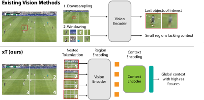
Figure 1: xT allows large images to be modeled end-to-end on contemporary GPUs without compromising on high frequency features or global context.

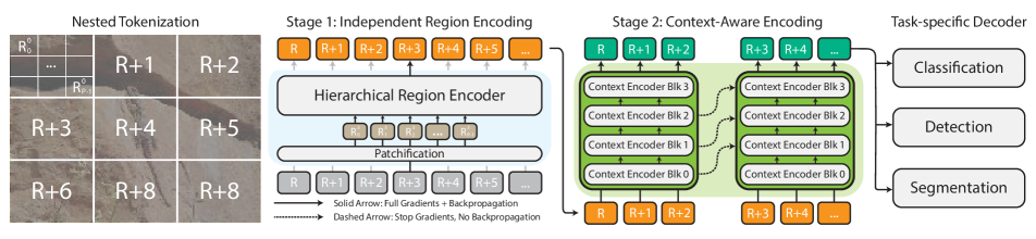
Figure 2: Overview of our methodology. xT provides a way for existing vision backbones trained on small images to work effectively with large images. The key is our nested tokenization of large images at multiple levels: at the region level as input $R^{0},\dots,R^{8}$ ($R$, …, $R+8$ for readability) for the region encoders, and then at the patch level $R^{i}_{0},\dots,R^{i}_{P-1}$ inside the encoders to understand local details. The image regions then undergo independent, hierarchical encoding, by passing through a vision backbone that serves as a region encoder. Hierarchical region encoders result in down-sampled features which, when combined with context encoders, allows us to process more regions at once than typically possible. One such context encoder, Transformer-XL, is illustrated in Stage 2. It recurrently processes previous prior sequence tokens using cross attention, extending its context range significantly with depth. The resulting sequence has assimilated both local and global context and is finally fed to a task-specific decoder.

We introduce xT, a framework by which myopic vision backbones can effectively integrate local and global context over large images. In particular,we tackle both issues of quadratically-increasing GPU memory utilization and the integration of context across very large images. We achieve this by improving the strengths of hierarchical vision backbones [21, 30] through nested tokenization of images and processing resulting features with long-sequence models, such as Transformer-XL and Mamba [3, 9], from the field of natural language processing. xT matches and beats the performance of competitive large image architectures on multiple downstream tasks that require large visual contexts such as segmentation, detection, and classification. We demonstrate results on a variety of downstream tasks and achieve up to an 8.6% gain in accuracy on classification tasks and an 11.6 increase in $F_{1}$ score on context-dependent segmentation.

2 Related Works

Modeling large images

Many prior works have attempted to model large images. These approaches fall into one of two buckets: 1) multi-pass hierarchical or cascading approaches and 2) sliding windows combined with some suppression mechanism. Dalal and Triggs famously utilized a sliding window approach for robust object recognition in their work on histograms of oriented gradients [4]. R-CNN [7] classified proposals generated by selective search in a cascade, resulting in a slow, albeit effective detector that worked for large images. Gadermayr, et. al. [6] proposed a cascading convolutional neural network (CNN) where regions of interest (RoI) are first segmented using low resolution imagery. These RoI are used to refine the segmentation mask using high resolution imagery.  [42] implement a multi-scale vision transformer architecture which outputs a feature pyramid combined with a linear attention mechanism.

As demonstrated by prior work, there are inherent benefits to using hierarchical backbones when attempting to represent multi-scale features, so all of our experiments are done with them. The xT framework is agnostic to the style of vision backbone used for feature extraction.

Assessing global understanding

Methods that aim to improve the handling of high-resolution or large images rarely benchmark their methods on real-world, large image datasets. For example, both [42] and [39] are ViT architectures with non-global attention to better model large images. However, both works experiment on datasets such as ImageNet which is comprised of images of $224\times 224$ pixels large.

Other evaluation methods rely on naïve data processing techniques such as cropping medium-sized images from Cityscapes into smaller chunks and independently stitching the outputs together [11], or center-cropping a $224\times 224$ patch from a larger (yet objectively small) ImageNet image [36]. Ultimately, these approaches are sensitive to changes in test-time resolution, though representation learning methods exist to rectify this issue [26].

Real-world classification and segmentation datasets that are heavily dependent on their surroundings, or in cases where the object that needs to be modeled is a small fraction of the overall image, would benefit from better integration of global context. Myopic vision encoders which utilize a windowing approach may fail at large objects in detection tasks as objects will span multiple windows.

We evaluate on real-world datasets such as xView3-SAR [25], a dataset where the average image is $29,400\times 24,400$ pixels large, and iNaturalist 2018 [34], where the entire $800\times 800$ image is utilized at once for evaluation. We also evaluate on the standard MS-COCO dataset for direct comparison to vision backbones built for smaller images.

Learning global context

Convolutional neural networks operate over images in sliding windows defined by the size of the kernels used for convolution. However, convolutions do not inherently aggregate information from surrounding windows. Following seminal work by Hubel and Wiesel [17] and Koenderink and Van Doorn [18] on feature pooling in the visual cortex, LeCun, et. al. [19] introduced “average pooling” into CNNs as a context aggregation mechanism. Dilated convolutions as implemented by Yu and Kolun [40] further increased the receptive field of CNNs.

Some models treat memory as an explicit, external component of the model. Neural Turing machines and memory networks  [8, 37] learn an access mechanism to read/write from a fixed-size memory matrix that is external to the backbone itself. More recently, MeMViT [38] extends this concept to sequences of images by caching and compressing activations from prior sequences with attention as a learned access mechanism.

Transformers and vision transformers [35, 5], consisting of stacked attention layers [1], are able to maintain context over a fixed number of tokens. Prior works attempt to address limitations in attention via approaches such as factorization and adaptive masking [2, 32]. Notably, the Transformer-XL [3] efficiently passes context over a large number of tokens by recycling state over recurring input segments.

Recurrent neural networks (RNNs) [16, 28] addressed context over long sequences by recurrently passing hidden states over a fixed set of time steps but suffered from catastrophic foregetting [14]. Subsequent work on long short-term memory [15] tackled this issue via gating. Structured state space models (SSMs) [10] have re-emerged recently as a viable successor to RNNs. Of the SSM family of models, the Mamba [9] architecture presents a selection mechanisms for state spaces allowing it to generalize to large sequence lengths.

xT extracts features from windows across a large image iteratively using a vision backbone. These features are fed into a shallow context encoder which integrates local context globally, effectively increasing the receptive field of the vision backbone across the entire image while staying within memory and parameter limits.

3 Background

In this section, we briefly summarize the needed background for methods used in our work.

3.1 Long-Context Models as Context Encoders

xT utilizes long-context models originally designed for text in order to mix information across large images. These methods extend the context length beyond the typical limit of transformers. Below we briefly review two techniques which we build upon as our context encoders: Transformer-XL [3] and Mamba [9].

Transformer-XL

uses recurrence to pass prior information to future windows via prior hidden states. This effect propagates through depth, so an $N$-layer transformer capable of taking a length $L$ sequence can be easily extended to handle a sequence of length $NL$.

Each hidden state $\mathbf{h}_{\tau}^{n}$ of layer $n$ for sequence $\tau$ is computed from the previous layer hidden states $\mathbf{h}_{\tau-1}^{n-1}$ and $\mathbf{h}_{\tau}^{n-1}$ as

$$\tilde{\mathbf{h}}_{\tau}^{n} =[\text{SG}(\mathbf{h}_{\tau-1}^{n-1})\circ\mathbf{h}_{\tau}^{n-1}]$$

$$\mathbf{q}_{\tau}^{n},\mathbf{k}_{\tau}^{n},\mathbf{v}_{\tau}^{n} =\mathbf{h}_{\tau}^{n-1}W_{q}^{\top},\tilde{\mathbf{h}}_{\tau}^{n}W_{k}^{\top},\tilde{\mathbf{h}}_{\tau}^{n}W_{v}^{\top}$$

$$\mathbf{h}_{\tau}^{n} =\text{Transformer}(\mathbf{q}_{\tau}^{n},\mathbf{k}_{\tau}^{n},\mathbf{v}_{\tau}^{n})$$ (1)

where SG stands for a stop gradient. This is the same as the original Transformer, except that the keys and values $\mathbf{k}_{\tau}^{n},\mathbf{v}_{\tau}^{n}$ are computed using the previous sequence’s hidden state $\mathbf{h}_{\tau-1}^{n-1}$ in addition to the current sequence’s hidden state $\mathbf{h}_{\tau}^{n-1}$ using cross attention. This mechanism allows for the recurrence of the hidden states $\mathbf{h}_{\tau}^{n}$ across layers. The application of a stop gradient between sequences lets information be propagated without suffering the memory costs incurred with full sequence backpropagation.

State Space Models

State space models [10, 24] have been re-discovered recently as a potential replacement for transformers in long-sequence modeling. These models can be formulated as ordinary differential equations of the form

$$\frac{dh(t)}{dt} =Ah(t)+Bx(t)$$

$$y(t) =Ch(t)+Dx(t)$$ (2)

where $x(t)\in\mathbb{R}$ is the input signal and $y(t)\in\mathbb{R}$ is the output signal. Practically, this is computed through a discretization of the ODE via the zero-order hold (ZOH) rule:

$$\bar{A} =\exp(\Delta A)$$

$$\bar{B} =(\Delta A)^{-1}(\exp(\Delta A)-I)\cdot\Delta B$$

$$h(t) =\bar{A}h_{t-1}+\bar{B}x_{t}$$ (3)

$$y_{t} =Ch_{t}$$ (4)

Mamba [9] is a new state space model that introduces a selective scan mechanism that allows time-varying parameterizations. Mamba theoretically carries context across very long sequences without any loss in accuracy and is implemented efficiently using custom CUDA kernels.

3.2 Linear attention mechanism

A standard transformer block with multi-headed self attention requires quadratic memory with respect to sequence length $L$ for fully global context. This is not ideal in the face of limited GPU memory. HyperAttention [12] is an attention mechanism with near-linear complexity with respect to sequence length. It reduces the complexity of naive attention by first finding large entries of the attention matrix using Locality Sensitive Hashing (LSH). These dominant entries, combined with another randomly sampled subset from the matrix, are then used to approximate output of naive attention. This approach is particular helpful when the long range context correspondences are sparse.

4 Methodology

Our goal for xT is to demonstrate a simple framework for allowing existing methods to process large images in a memory efficient and contextual manner. We achieve this through an iterative, two-stage design. First, images are tokenized hierarchically (Section 4.1) before being independently featurized by a region encoder with a limited context window (Section 4.2). Then, a lightweight context encoder incorporates context globally across this sequence of features (Section 4.3), which then gets passed to the task-specific decoders. Our overall pipeline is illustrated in Figure 2.

4.1 Nested Tokenization

Given a large input image of shape $\alpha H\times\beta W$, we first subdivide the image into $H\times W$ regions so that our region encoder can adequately process them. Each region $R^{i}$ is further patchified into $P$ patches, $R^{i}_{0},\dots,R^{i}_{P-1}$, by the region encoder backbone in order to extract features for each region. The regions are non-overlapping and zero-padded in instances when the region size, $H\times W$, does not evenly divide the image size.

Typically our images and regions are square, so we use a simplified notation to denote our pipeline parameters. We refer to a pipeline which receives images of size $\alpha R\times\alpha R$ and subdivides them into $R\times R$ regions as an $\alpha R/R$ setup. Standard setups are $512/256$, or $4096/512$, in which we split our image into $2\times 2$ and $8\times 8$ tiles respectively.

4.2 Region Encoder

We start with an image model which is trained for a typical size of small images $H\times W$, usually $224\times 224$ or $256\times 256$. The region encoder independently generates feature maps for each region $R^{i}_{1...P}$. Our region encoders are hierarchical vision transformers in which the sequence length decreases from the beginning of the process, and is also less than the equivalent length produced by isotropic ViTs [5]. We are therefore able to combine more region features together than we would with other architectures, as our sequence length is reduced by $4\times$ or greater.

When GPU memory allows, we compute features for all regions simultaneously. However, when the image is too large such that all of its constituent regions cannot fit into GPU memory, we process each region sequentially.

4.3 Context Encoder

The output region features are concatenated in row major order to form a sequence. In the xT framework, the context encoder is a lightweight sequence-to-sequence model that attends across long sequence lengths. Critically, we constrain the context encoder to have a near-linear memory and time cost. This design allows xT to see many other regions of the large image which otherwise would not be feasible in memory. This significantly extends the receptive field of existing vision models with a marginal increase in memory cost and the number of parameters.

Our method acts primarily in two settings: when our sequence of region features fits entirely within the context encoder’s context length, and when it does not. In the first, we simply process everything at once. We use standard 2D positional embeddings which are added to the nested region features.

We experiment with three context encoders with linear “attention” mechanisms: a LLaMA-style [33] architecture using HyperAttention (referred to as Hyper), and Mamba. These two settings are called ⟨xT⟩ Hyper and ⟨xT⟩ Mamba, where ⟨xT⟩ is an operator joining the choice of region encoder with context encoder.

When our input sequence does not fit in the entire context length, we need to additionally compress our regions to maintain contextual information for future regions. We experiment with a derivative of Transformer-XL that utilizes HyperAttention, a form of linear attention, and absolute positional embeddings instead. We denote this setting as ⟨xT⟩ XL. At the time of writing, Mamba does not have an efficient kernel for implementing an XL-style recurrence, so we cannot apply Mamba to this setting.

Effective Receptive Field Calculations

We provide calculations of the effective receptive field for the Swin ⟨xT⟩ XL setup. This is further ablated in Section 7.1.

In the context encoder, we concatenate the features of $C$ regions into one “chunk” as our features are both smaller than the inputs from the hierarchical regional encoder. The Transformer-XL context encoder additionally has reduced attention memory requirements from using HyperAttention, further improving the number of regions that fit into one “chunk”. Each region attends to all other regions in this chunk, and they also have access to the previous chunk’s hidden states for more context flow through the model. Context scales as a function of depth in Transformer-XL.

Consequently, we can calculate the context enhancement we achieve beyond just a standard model query on a small image. If we use a region encoder with input size $R$ (typically 256) and receive a large image of size $\alpha R\times\beta R$, then we will have a total of $\alpha\beta$ regions available for our context encoder. Then we increase our context from increased chunk sizes by a factor of $C$, and also increase it from our recurrent memory by a factor of $N$, the depth of the context model. These values are calculated in Table 1 and further visualized in Figure 4.

In total, our context is multiplied by $\alpha\beta NC$. However, note that there is a trade-off between $\alpha\beta$ and $C$, as increasing the size of our input image limits the chunk sizes that we can create from the region features.

Model	Input (px)	Region (px)	XL Layers	Context
Swin-B	256	256	-	65,536
Swin-B	512	512	-	65,536
Swin-B ⟨xT⟩ XL	512	256	1	131,072
Swin-B ⟨xT⟩ XL	512	256	2	196,608
Swin-B ⟨xT⟩ XL	4096	256	2	786,432

Table 1: The effective context length (in pixels) is calculated for Swin-B versus Swin-B ⟨xT⟩ XL. Context is fixed for Swin while it grows as a function of region size and the number of Transformer-XL layers for Swin ⟨xT⟩ XL.

5 Experiments

Settings

We aim to demonstrate the efficacy of xT across the most common vision tasks: classification, detection, and segmentation. To do so, we pick a representative and challenging benchmark dataset in each domain for experimentation.

We focus on iNaturalist 2018 [34] for classification, xView3-SAR [25] for segmentation, and MS-COCO [20] for detection. Since iNaturalist 2018 is a massive dataset, we focus on the Reptilia super-class, the most challenging subset available in the benchmark [34]. xView3-SAR is a difficult segmentation dataset for two reasons: it is comprised of extremely large images that are 29,400$\times$24,400 pixels large on average, and the objects in the dataset are heavily influenced by their non-local surroundings. Lastly, MS-COCO is used for evaluation of detection and to serve as a common baseline across prior work.

Metrics

We measure top-1 accuracy for classification. For detection, we measure mean average precision (mAP) along with mAP_Large. mAP_Large is of specific interest since large objects in large images cross multiple region boundaries, resulting in a challenging training and evaluation problem. Segmentation is measured in two ways: aggregate $F_{1}$ score for segmentation of any object in the image, and close-to-shore $F_{1}$ score for objects that are “close to the shoreline”. xView3-SAR is comprised of synthetic aperture radar images which demonstrate unique artifacts around busy areas not found in typical vision benchmarks. Particularly, objects within 2km of the shoreline are impacted heavily by a shoreline that may not be visible in crops around the object.

5.1 Classification

Model	Top-1 Acc	Size(s)	Param	Mem (GB)
Swin-T	53.76	256	31M	0.30
Swin-T ⟨xT⟩ Hyper	52.93	256/256	47M	0.31
Swin-T ⟨xT⟩ Hyper	60.56	512/256	47M	0.29
Swin-T ⟨xT⟩ XL	58.92	512/256	47M	0.17
Swin-T ⟨xT⟩ Mamba	61.97	512/256	44M	0.29
Swin-S	58.45	256	52M	0.46
Swin-S ⟨xT⟩ Hyper	57.04	256/256	69M	0.46
Swin-S ⟨xT⟩ Hyper	63.62	512/256	69M	0.46
Swin-S ⟨xT⟩ XL	62.68	512/256	69M	0.23
Swin-S ⟨xT⟩ Mamba*	-	-	-	-
Hiera-B	48.60	224	54M	0.26
Hiera-B+	50.47	224	73M	0.33
Hiera-B ⟨xT⟩ Hyper	57.20	448/224	70M	0.21
Swin-B	58.57	256	92M	0.50
Swin-B ⟨xT⟩ Hyper	55.52	256/256	107M	0.61
Swin-B ⟨xT⟩ Hyper	64.08	512/256	107M	0.74
Swin-B ⟨xT⟩ XL	62.09	512/256	107M	0.39
Swin-B ⟨xT⟩ Mamba	63.73	512/256	103M	0.58
Swin-L	68.78	256	206M	0.84
Swin-L ⟨xT⟩ Hyper	67.84	256/256	215M	1.06
Swin-L ⟨xT⟩ Hyper	72.42	512/256	215M	1.03
Swin-L ⟨xT⟩ XL	73.47	512/256	215M	0.53
Swin-L ⟨xT⟩ Mamba	73.36	512/256	212M	1.03

Table 2: Comparison to prior methods on iNaturalist Reptilia Classification. Our methods improve on prior works significantly, showing that previous methods still fail to integrate global context. Memory is per base region size, which is fixed for each comparison. *Custom Mamba CUDA kernels are incompatible with Swin-S at this time.

We utilize the SwinV2 [22] and Hiera [30] families of hierarchical vision models as the region encoders for the classification experiments. All variants of Swin—tiny, small, base, and large—are pretrained on the ImageNet-1k [29] dataset. Both Hiera-B and Hiera-B+ are initialized with MAE [13] pre-trained/ImageNet-1k fine-tuned weights. Two layers of Hyper or four layers of Mamba are used as the context encoder, intialized randomly.

We train end-to-end on the Reptilia subset of iNaturalist 2018 for 100 epochs using the AdamW optimizer ($\beta_{1}=0.9$, $\beta_{2}=0.999$, $\epsilon=1\times 10^{-8}$) using cosine learning rate decay schedule. Swin-T, Swin-S, Hiera-B/+, and their xT variants use a base learning rate of $1\times 10^{-4}$ while Swin-B, Swin-L, and their xT variants use a base learning rate of $1\times 10^{-5}$. xT’s nested tokenization scheme is represented as two values, e.g. 512/256, where the first value is the size of the regions extracted from the input image and the second value is the input size expected by the region encoder.

Table 2 contains results for variants of Swin, Hiera, and their xT variants on iNaturalist-Reptilia. Particularly, we demonstrate xT’s results as a function of region/input size and type of context encoder. xT outperforms their comparable baselines by significant margins.

We show in Figure 3 that xT sets a new accuracy-parameter frontier when compared against existing methods.

5.2 Segmentation on xView3-SAR

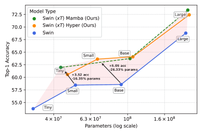
Figure 3: xT improves upon the accuracy-parameter frontier of existing methods for high-resolution classification on iNaturalist using nested tokenization on top of the origin architecture for larger context. See Table 2 for detailed comparisons.

We evaluate xT on the xView3-SAR [25] dataset, a large, real-world dataset of satellite imagery for the task of detecting dark vessels. The average image size is $29,400\times 24,400$ pixels large, so accurate detections require using long-range geospatial context to make decisions. We calculate two metrics on xView3-SAR: the aggregate and overall detection $F_{1}$ scores which reflect general task proficiency, and of most importance, the close-to-shore detection $F_{1}$, which requires detecting vessels close to the shore by using predominant shoreline information.

We adopt the same setup as prior methods [31], tackling the problem as a segmentation and regression problem using a standard encoder-decoder architecture for dense prediction. In our case, we adopt Swin Transformer v2 [22] pretrained on ImageNet-1k as our region encoder and use a UNet-style decoder [27]. We regress the centers of objects as Gaussians and vessels as binary masks.

We test Swin-Tiny, Swin-Small, and Swin-Base, and their xT-variants using Transformer-XL as a context encoder with $N=4$ layers. The models are trained over encoder input sizes of $512$ and $1024$, which xT effectively boosts to 4096. At inference time, we take overlapping crops of the same size across the image and combine our predictions with some post-processing. We sweep our models over learning rates of $\{3\times 10^{-5},10^{-4},3\times 10^{-4},10^{-3},3\times 10^{-3}\}$ using AdamW (with the same hyperparameters as in Section 5.1) and report the validation numbers in Table 3.

While prior works tackle xView3 using smaller, lighter models like CNNs, ours opts to adapt transformers for the task, which is a relatively unexplored space for the type of images and data distributions present. Therefore, larger models are not always better, as observed in Table 3. However, xT always outperforms the corresponding non-context model, especially on the overall $F_{1}$ detection score, signaling our models broad ability to improve models on large context tasks. We do this while only introducing $5-10\%$ extra parameters, and thanks to our nested tokenization, the memory we utilize per region is much lower as we see multiple regions at once per pass.

Model	Shore$\uparrow$	Agg$\uparrow$	$F_{1}$ Score$\uparrow$	Param	Mem$\downarrow$	Input Size(s)
Swin-T	50.0	47.6	67.8	32.4	1.24	512
Swin-T	51.6	53.2	76.8	32.4	5.30	1024
Swin-T ⟨xT⟩ XL	47.5	49.4	81.2	36.9	0.47	4096/512
Swin-T ⟨xT⟩ XL	56.0	54.8	78.2	36.9	1.65	4096/1024
Swin-S	46.1	44.9	67.7	53.7	1.84	512
Swin-S	41.2	43.8	71.0	53.7	7.24	1024
Swin-S ⟨xT⟩ XL	50.2	48.1	75.3	58.3	0.54	4096/512
Swin-S ⟨xT⟩ XL	52.8	55.1	78.8	58.3	2.24	4096/1024
Swin-B	50.2	51.6	72.1	92.7	2.36	512
Swin-B	54.4	54.7	75.8	92.7	9.65	1024
Swin-B ⟨xT⟩ XL	52.4	51.5	76.4	97.4	0.70	4096/512
Swin-B ⟨xT⟩ XL	51.0	50.8	77.2	97.4	2.82	4096/1024

Table 3: Comparison to prior methods on xView3-SAR detection. We evaluate our methods on xView3-SAR, a dataset for dark vessel detection from satellite imagery. Our method improves on prior state of the art hierarchical transformers significantly while introducing few extra parameters and using less memory per region due to our efficient context encoder. This shows that prior works, expectedly, are unable to model long range visual contexts.

Model	mAP	mAPL	Input Size(s)
Swin-B-DINO	30.0	36.1	256
Swin-B-DINO	32.5	39.6	512
Swin-B-DINO ⟨xT⟩ Hyper	49.8	68.5	1333/256
Swin-B-DINO ⟨xT⟩ Hyper	50.9	70.6	1333/512

Table 4: Comparison with Swin-B on the COCO 2017 object detection task. We report mAP and $\text{mAP}_{\text{Large}}$ on val2017.

context	acc	param	mem
ViT	63.26	107M	0.73
Hyper	64.08	107M	0.74
Mamba	63.73	103M	0.58

(a)

model	depth	acc
Swin-T	1	86.38
	2	85.09
Swin-S	1	88.26
	2	88.03
Swin-B	1	89.08
	2	90.73
Swin-L	1	91.67
	2	94.48

(b)

model	size	acc	params
Swin-T	256	53.76	31M
	256/256	52.93	47M
	512/256	60.56	47M
Swin-L	256	68.78	206M
	256/256	67.84	215M
	512/256	72.42	215M

(c)

Table 5: Ablating xT design choices. We highlight our defaults in blue and bold the best numbers.

5.3 Object Detection

We use SwinV2 [22] as the backbone and adopt DINO [41] for the detection head. We follow the standard COCO 1x training schedule and train on MS-COCO for 12 epochs with the AdamW optimizer ($\beta_{1}=0.9$, $\beta_{2}=0.999$) and a learning rate of $1\times 10^{-3}$. The learning rate for the SwinV2 backbone is scaled by a factor of 0.1. The input is first padded to the nearest multiple of chip size first, and then chipped in the same way as Sec. 5.1. Each region is then processed by the region encoder independently. The outputs from Swin encoder are concatenated to form a global feature map of the entire image, which is then processed by the context encoder. The resulting sequence is passed to the DINO detection head.

When utilizing the commonly adopted windowing approach, large objects that span multiple windows are split apart. This is a challenging task for state-of-the-art vision models to handle. Following, we report mAP and $\text{mAP}_{\text{Large}}$ for our detection experiments on val2017 subset. Comparing with plainly using Swin, xT  achieves strong performance when compared with baselines.

6 Ablations

In this section, we ablate our design choices based on iNaturalist classification, particularly around our context encoder. The settings that we keep constant are that xT is run on 512/256 inputs, where we chunk our four regions together to create one sequence into our context encoder. As this usually fits in memory, we have no need to perform cross-chunk contextualizing as we do in xView.

6.1 Context Encoder Architecture

We tested ViT, Hyper, and Mamba as context encoders in the course of our classification experiments. These results are detailed LABEL:tab:ablation_context_backbone. iNaturalist 2018 resizes their images to $800\times 800$ pixels for training. These images can be modeled comfortably by ViT and benefit from full self-attention. However, both Hyper and Mamba both perform better than ViT as context encoders with the added benefit of having a much larger capacity for scale.

While Mamba has less parameters than both ViT and Hyper—up to 8% fewer parameters for Swin-T ⟨xT⟩ Mamba than for Swin-T ⟨xT⟩ Hyper—this difference disappears as the region encoder increases in size as seen in Table 2. Furthermore, the decrease in parameters ultimately has an insignificant impact on the peak memory usage of the overall xT model.

6.2 Context Encoder Depth

Crucial to our design is how deep our context encoder should be, as our goal is to keep it as lightweight as possible so its overhead is minimal. We find that an acceptable increase in parameters keeps the number of layers to either 1 or 2. As shown in Table LABEL:tab:context_encoder_depth, larger region encoders generally benefit from having deeper context encoders. The accuracy is the greatest when the depth is 2 for the largest model, and the trade-off is acceptable for the smallest model, being within 1 accuracy point, so we choose depth 2 as our default.

6.3 Resolution Size Matters

We revisit the central assumption of our work, which is if high resolution is essential for understanding. In Table LABEL:tab:resolution, we emphasize our results on iNaturalist which prove precisely that models previously did not take advantage of such context, and now do with xT. Comparing the Swin-T/L 256 run with Swin-T/L 256/256, which is our method taking in no context, our model actually does worse with extra parameters, likely due to non-functional parameters interfering with the model’s learning. However, once we increase our input image size by $4\times$ to $512/256$, our model is immediately able to take advantage of the context with no increase in parameters, boosting accuracy up by 4.6%-7.6%.

7 Discussion

7.1 Effective Receptive Field

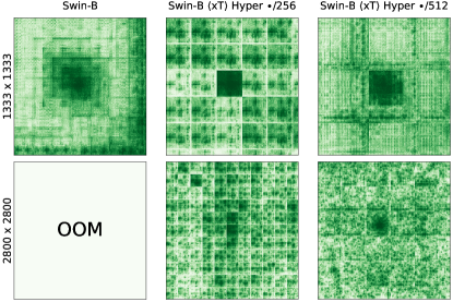
Figure 4: Effective receptive fields of Swin-B and Swin-B ⟨xT⟩ Hyper. The center feature from the last layer of region encoder is used to assess sensitivity to areas across the image. Darker green signifies greater sensitivity.

We empirically visualize the effective receptive field (ERF) [23] of xT  in Figure 4. The effective receptive field is computed by setting the gradient of one pixel in the final feature map to 1 while keeping the gradient of all other pixels as zero, and then computing the gradient with respect to the input image through a backward pass. The visualized image measures the magnitude of gradient with darker green areas demonstrating greater “sensitivity” and lighter areas demonstrating lower. We show that Swin Transformer has an ERF similar to a skewed Gaussian which vanishes quickly over distance. Comparatively, xT retains a more uniform distribution across the entire image. Since our nested tokenization approach is effectively a convolution, we see convolution-like artifacts in the ERF that are mitigated as region sizes get larger. This highlights the xT framework’s capacity at capturing and integrating long range context in large images.

7.2 Throughput

In lieu of FLOPS, which is difficult to standardize, hardware dependent, and an inconsistent measure of running time when using custom kernels, we instead report the throughput of our method and compare to prior works in Figure 5. For our comparisons, we use 40GB Nvidia A100 GPUs. As we work with multiple image resolutions at once, we calculate a throughput of regions/second, which is the number of encoder-sized regions we process per second.

On a per-model size comparison, our method drops in throughput slightly compared to prior methods (with the exception of the fastest size, Tiny). However, we are able to achieve large accuracy gains for this slight tradeoff which are much better than if we used a larger model from prior work instead. This demonstrates the benefit of our method in improving the frontier in modeling larger images efficiently.

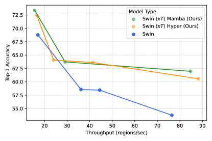
Figure 5: xT offers greatly increased accuracy per throughput. On iNaturalist classification, we find that our models only slightly diminished throughput (with the exception of Swin-T ⟨xT⟩ XL/Mamba) but achieved greater accuracies at each throughput threshold.

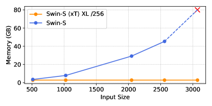
Figure 6: Swin rapidly goes out of memory (indicated by the red X) as images grow in size whereas xT retains near-constant memory cost. xT can scale to much larger images than the naïve usage of a vision backbone.

7.3 Memory Growth

Modern vision backbone, such as Swin, rapidly run out-of-memory near-quadratically as the image size increases. In Figure 6, we show how the xT framework effectively removes this quadratic memory growth, allowing the model to reason over large images end-to-end. Thanks to our chunking design, our method incurs minimal extra memory when we increase our input size as we recurrently store previous regions as context for future context-aware encoding.

8 Conclusion

Large images have been the norm for the past decade in consumer and professional domains. Yet, state-of-the-art methods in computer vision still limit themselves to modeling small images by throwing away valuable information via down-sampling and cropping. Large images from the real world contain a wealth of information that often require context across long distances to properly make sense of.

In this work, we introduce xT, a framework through which vision models trained to handle small images can cheaply integrate larger context over large images. xT achieves significant gains in downstream tasks such as classification, detection, and segmentation on real-world datasets. By offering a simple framework by which vision researchers can effectively model large images, we aim to widen the types of data and tasks vision researchers aim to solve.

References

- Bahdanau et al. [2016] Dzmitry Bahdanau, Kyunghyun Cho, and Yoshua Bengio. Neural Machine Translation by Jointly Learning to Align and Translate, 2016.
- Child et al. [2019] Rewon Child, Scott Gray, Alec Radford, and Ilya Sutskever. Generating Long Sequences with Sparse Transformers, 2019.
- Dai et al. [2019] Zihang Dai, Zhilin Yang, Yiming Yang, Jaime Carbonell, Quoc Le, and Ruslan Salakhutdinov. Transformer-XL: Attentive Language Models beyond a Fixed-Length Context. In Proceedings of the 57th Annual Meeting of the Association for Computational Linguistics, pages 2978–2988, Florence, Italy, 2019. Association for Computational Linguistics.
- Dalal and Triggs [2005] Navneet Dalal and Bill Triggs. Histograms of Oriented Gradients for Human Detection. IEEE Computer Society Conference on Computer Vision and Pattern Recognition, 2005.
- Dosovitskiy et al. [2020] Alexey Dosovitskiy, Lucas Beyer, Alexander Kolesnikov, Dirk Weissenborn, Xiaohua Zhai, Thomas Unterthiner, Mostafa Dehghani, Matthias Minderer, Georg Heigold, Sylvain Gelly, Jakob Uszkoreit, and Neil Houlsby. An Image is Worth 16x16 Words: Transformers for Image Recognition at Scale. In International Conference on Learning Representations, 2020.
- Gadermayr et al. [2019] Michael Gadermayr, Ann-Kathrin Dombrowski, Barbara Mara Klinkhammer, Peter Boor, and Dorit Merhof. CNN cascades for segmenting sparse objects in gigapixel whole slide images. Computerized Medical Imaging and Graphics, 71:40–48, 2019.
- Girshick et al. [2014] Ross Girshick, Jeff Donahue, Trevor Darrell, and Jitendra Malik. Rich Feature Hierarchies for Accurate Object Detection and Semantic Segmentation. In Proceedings of the IEEE Conference on Computer Vision and Pattern Recognition, pages 580–587, 2014.
- Graves et al. [2014] Alex Graves, Greg Wayne, and Ivo Danihelka. Neural Turing Machines, 2014.
- Gu and Dao [2023] Albert Gu and Tri Dao. Mamba: Linear-time sequence modeling with selective state spaces. arXiv preprint arXiv:2312.00752, 2023.
- Gu et al. [2022] Albert Gu, Karan Goel, and Christopher Ré. Efficiently modeling long sequences with structured state spaces. In The International Conference on Learning Representations (ICLR), 2022.
- Gu et al. [2021] Jiaqi Gu, Hyoukjun Kwon, Dilin Wang, Wei Ye, Meng Li, Yu-Hsin Chen, Liangzhen Lai, Vikas Chandra, and David Z. Pan. Multi-Scale High-Resolution Vision Transformer for Semantic Segmentation, 2021.
- Han et al. [2023] Insu Han, Rajesh Jayaram, Amin Karbasi, Vahab Mirrokni, David P Woodruff, and Amir Zandieh. Hyperattention: Long-context attention in near-linear time. arXiv preprint arXiv:2310.05869, 2023.
- He et al. [2022] Kaiming He, Xinlei Chen, Saining Xie, Yanghao Li, Piotr Dollar, and Ross Girshick. Masked Autoencoders Are Scalable Vision Learners. In 2022 IEEE/CVF Conference on Computer Vision and Pattern Recognition (CVPR), pages 15979–15988, New Orleans, LA, USA, 2022. IEEE.
- Hochreiter [1991] Sepp Hochreiter. Untersuchungen zu dynamischen neuronalen Netzen. 1991.
- Hochreiter and Schmidhuber [1997] Sepp Hochreiter and Jürgen Schmidhuber. Long Short-Term Memory. Neural Computation, 9(8):1735–1780, 1997.
- Hopfield [1982] J J Hopfield. Neural networks and physical systems with emergent collective computational abilities. Proceedings of the National Academy of Sciences, 79(8):2554–2558, 1982.
- Hubel and Wiesel [1962] D. H. Hubel and T. N. Wiesel. Receptive fields, binocular interaction and functional architecture in the cat’s visual cortex. The Journal of Physiology, 160(1):106–154, 1962.
- Koenderink and Van Doorn [1999] Jan J. Koenderink and Andrea J. Van Doorn. The Structure of Locally Orderless Images. International Journal of Computer Vision, 31(2):159–168, 1999.
- LeCun et al. [1989] Yann LeCun, Bernhard Boser, John Denker, Donnie Henderson, R. Howard, Wayne Hubbard, and Lawrence Jackel. Handwritten Digit Recognition with a Back-Propagation Network. In Advances in Neural Information Processing Systems. Morgan-Kaufmann, 1989.
- Lin et al. [2015] Tsung-Yi Lin, Michael Maire, Serge Belongie, Lubomir Bourdev, Ross Girshick, James Hays, Pietro Perona, Deva Ramanan, C. Lawrence Zitnick, and Piotr Dollár. Microsoft COCO: Common Objects in Context, 2015.
- Liu et al. [2021] Ze Liu, Yutong Lin, Yue Cao, Han Hu, Yixuan Wei, Zheng Zhang, Stephen Lin, and Baining Guo. Swin Transformer: Hierarchical Vision Transformer using Shifted Windows. In 2021 IEEE/CVF International Conference on Computer Vision (ICCV), pages 9992–10002, Montreal, QC, Canada, 2021. IEEE.
- Liu et al. [2022] Ze Liu, Han Hu, Yutong Lin, Zhuliang Yao, Zhenda Xie, Yixuan Wei, Jia Ning, Yue Cao, Zheng Zhang, Li Dong, Furu Wei, and Baining Guo. Swin transformer v2: Scaling up capacity and resolution. In International Conference on Computer Vision and Pattern Recognition (CVPR), 2022.
- Luo et al. [2016] Wenjie Luo, Yujia Li, Raquel Urtasun, and Richard Zemel. Understanding the effective receptive field in deep convolutional neural networks. Advances in neural information processing systems, 29, 2016.
- Nguyen et al. [2022] Eric Nguyen, Karan Goel, Albert Gu, Gordon W. Downs, Preey Shah, Tri Dao, Stephen A. Baccus, and Christopher Ré. S4nd: Modeling images and videos as multidimensional signals using state spaces. Advances in Neural Information Processing Systems, 35, 2022.
- Paolo et al. [2022] Fernando Paolo, Tsu-ting Tim Lin, Ritwik Gupta, Bryce Goodman, Nirav Patel, Daniel Kuster, David Kroodsma, and Jared Dunnmon. xView3-SAR: Detecting Dark Fishing Activity Using Synthetic Aperture Radar Imagery. Advances in Neural Information Processing Systems, 35:37604–37616, 2022.
- Reed et al. [2023] Colorado J Reed, Ritwik Gupta, Shufan Li, Sarah Brockman, Christopher Funk, Brian Clipp, Kurt Keutzer, Salvatore Candido, Matt Uyttendaele, and Trevor Darrell. Scale-MAE: A Scale-Aware Masked Autoencoder for Multiscale Geospatial Representation Learning. 2023 IEEE/CVF International Conference on Computer Vision (ICCV), pages 4065–4076, 2023.
- Ronneberger et al. [2015] Olaf Ronneberger, Philipp Fischer, and Thomas Brox. U-net: Convolutional networks for biomedical image segmentation. In Medical Image Computing and Computer-Assisted Intervention–MICCAI 2015: 18th International Conference, Munich, Germany, October 5-9, 2015, Proceedings, Part III 18, pages 234–241. Springer, 2015.
- Rumelhart and McClelland [1987] David E. Rumelhart and James L. McClelland. Learning Internal Representations by Error Propagation. In Parallel Distributed Processing: Explorations in the Microstructure of Cognition: Foundations, pages 318–362. MIT Press, 1987.
- Russakovsky et al. [2015] Olga Russakovsky, Jia Deng, Hao Su, Jonathan Krause, Sanjeev Satheesh, Sean Ma, Zhiheng Huang, Andrej Karpathy, Aditya Khosla, Michael Bernstein, et al. Imagenet large scale visual recognition challenge. International journal of computer vision, 115:211–252, 2015.
- Ryali et al. [2023] Chaitanya Ryali, Yuan-Ting Hu, Daniel Bolya, Chen Wei, Haoqi Fan, Po-Yao Huang, Vaibhav Aggarwal, Arkabandhu Chowdhury, Omid Poursaeed, Judy Hoffman, Jitendra Malik, Yanghao Li, and Christoph Feichtenhofer. Hiera: A hierarchical vision transformer without the bells-and-whistles. In Proceedings of the 40th International Conference on Machine Learning, pages 29441–29454, Honolulu, Hawaii, USA, 2023. JMLR.org.
- Seferbekov [2022] Selim Seferbekov. xView3 2nd place solution. https://github.com/DIUx-xView/xView3_second_place, 2022.
- Sukhbaatar et al. [2019] Sainbayar Sukhbaatar, Edouard Grave, Piotr Bojanowski, and Armand Joulin. Adaptive Attention Span in Transformers. In Proceedings of the 57th Annual Meeting of the Association for Computational Linguistics, pages 331–335, Florence, Italy, 2019. Association for Computational Linguistics.
- Touvron et al. [2023] Hugo Touvron, Thibaut Lavril, Gautier Izacard, Xavier Martinet, Marie-Anne Lachaux, Timothée Lacroix, Baptiste Rozière, Naman Goyal, Eric Hambro, Faisal Azhar, Aurelien Rodriguez, Armand Joulin, Edouard Grave, and Guillaume Lample. LLaMA: Open and Efficient Foundation Language Models, 2023.
- Van Horn et al. [2018] Grant Van Horn, Oisin Mac Aodha, Yang Song, Yin Cui, Chen Sun, Alex Shepard, Hartwig Adam, Pietro Perona, and Serge Belongie. The iNaturalist Species Classification and Detection Dataset. In 2018 IEEE/CVF Conference on Computer Vision and Pattern Recognition, pages 8769–8778, Salt Lake City, UT, 2018. IEEE.
- Vaswani et al. [2017] Ashish Vaswani, Noam Shazeer, Niki Parmar, Jakob Uszkoreit, Llion Jones, Aidan N Gomez, Łukasz Kaiser, and Illia Polosukhin. Attention is All you Need. In Advances in Neural Information Processing Systems. Curran Associates, Inc., 2017.
- Wang et al. [2021] Wenhai Wang, Enze Xie, Xiang Li, Deng-Ping Fan, Kaitao Song, Ding Liang, Tong Lu, Ping Luo, and Ling Shao. Pyramid Vision Transformer: A Versatile Backbone for Dense Prediction without Convolutions, 2021.
- Weston et al. [2015] Jason Weston, Sumit Chopra, and Antoine Bordes. Memory Networks, 2015.
- Wu et al. [2022] Chao-Yuan Wu, Yanghao Li, Karttikeya Mangalam, Haoqi Fan, Bo Xiong, Jitendra Malik, and Christoph Feichtenhofer. MeMViT: Memory-Augmented Multiscale Vision Transformer for Efficient Long-Term Video Recognition. In Proceedings of the IEEE/CVF Conference on Computer Vision and Pattern Recognition, pages 13587–13597, 2022.
- Yang et al. [2022] Chenhongyi Yang, Jiarui Xu, Shalini De Mello, Elliot J. Crowley, and Xiaolong Wang. GPViT: A High Resolution Non-Hierarchical Vision Transformer with Group Propagation. In The Eleventh International Conference on Learning Representations, 2022.
- Yu and Koltun [2016] Fisher Yu and Vladlen Koltun. Multi-Scale Context Aggregation by Dilated Convolutions, 2016.
- Zhang et al. [2022] Hao Zhang, Feng Li, Shilong Liu, Lei Zhang, Hang Su, Jun Zhu, Lionel M. Ni, and Heung-Yeung Shum. Dino: Detr with improved denoising anchor boxes for end-to-end object detection, 2022.
- Zhang et al. [2021] Pengchuan Zhang, Xiyang Dai, Jianwei Yang, Bin Xiao, Lu Yuan, Lei Zhang, and Jianfeng Gao. Multi-Scale Vision Longformer: A New Vision Transformer for High-Resolution Image Encoding, 2021.