Discrete time-crystals in linear potentials

Abstract

Discrete time crystalline (DTC) phases have attracted significant theoretical and experimental attention in the last few years. Such systems require a seemingly impossible combination of non-adiabatic driving and a finite-entropy long-time state, which is, however, possible in non-ergodic systems. Previous works have often relied on disorder for the required non-ergodicity; here, we describe the construction of a discrete time crystal (DTC) phase in non-disordered, non-integrable Ising-type systems. After discussing the conditions for interacting and periodically driven systems to display such phases in general, we propose a concrete model and then provide approximate analytical arguments and direct numerical evidence that it satisfies the conditions and displays a DTC phase robust to local periodic perturbations.

Introduction.—The study of dynamical phases of matter has been one of the most fruitful directions in many-body physics over the last few years. Time crystals, in which both spatial and temporal symmetries are spontaneously broken, constitute one of the most recognisable examples. Conceptually, these are attractive for two reasons: Firstly, they are genuine out of equilibrium phases of matter, impossible at equilibrium [1]. Secondly, they surf the very edge of the second law of thermodynamics: They simultaneously require a system that is non-adiabatically perturbed, which would usually result in entropic increase (heating) [2, 3, 4], but at the same time the system must not heat up to a featureless infinite temperature state, since then no spatiotemporal structures will emerge. These apparently contradictory requirements may be simultaneously satisfied in a way that we will explain in this work, and that was first used in a different, disordered system earlier [5].

So far, most DTCs have been found in systems that are temporally perturbed, usually periodically (“Floquet systems”). Such systems generically heat up towards a uniform, featureless state unfavourable to nontrivial effects [2, 3, 4]. Obtaining nontrivial effects therefore requires consideration of finite-time properties (prethermal physics [6, 7, 8, 9]) or non-ergodic systems which do not heat up when driven.

The first approach taken to break ergodicity was using disorder [10, 11]. It allowed for driving without heating, and is often called Floquet Many-Body Localization (Floquet-MBL) [2, 12, 13]. Not long afterwards Discrete Time Crystal (DTC) phases were proposed [5, 14, 15] and observed [16, 17, 18, 19, 20] in Floquet systems.

It was later realised that a tilted potential (uniform force) results in localisation and therefore ergodicity breaking in certain interacting systems [21, 22, 23]. This effect, which is closely related to Bloch oscillations, has been known for many years for noninteracting systems [24, 25]. For interacting systems the situation is somewhat more complicated than expected, since any finite system with a purely reflection-symmetric (such as linear) potential is not localised [26, 27]. It has already been established that such systems remain localised under periodic driving [28, 29], and show certain features of DTC phase [30, 31].

In this Letter we show how to construct a DTC using a a linear potential to prevent ergodicity and the system’s heat death. After discussing a set of features necessary for stable temporal order for a simple prototypical model we discuss its stability, and finally provide numerical support for our conclusions.

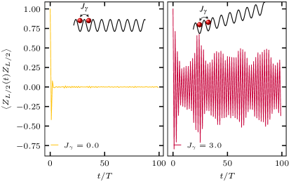
Figure 1: Short-time dynamics of a local correlation function $\left\langle\hat{Z}_{L/2}\left(t\right)\hat{Z}_{L/2}\right\rangle$ for constant interactions (left), and tilted interactions (right) between the nearby spins. The parameters used for this simulation are $L=10$, $h=0.5$, $J_{0}=1$, $V=0.5$, $\theta/\pi=-0.1$ and $T=1$.

Time-liquids.—We define time-liquids (TL) as systems with a static or periodic Hamiltonians whose local observables approach a constant or a periodic function, correspondingly, at the thermodynamic limit and after infinitely long time [32, 33, 34, 35, 36, 3] . As such, their long time dynamics is invariant with respect to the same time-translation generator as the Hamiltonian . The thermodynamic limit is essential since the observable in any finite closed system will fluctuate in time. Infinite time limit is needed, since the initial condition itself breaks time-translation symmetry and therefore for any finite time, the temporal dependence of an observable cannot be expected to be time-translationally invariant.

For static time-liquids, the stationary value of an observable corresponds to its infinite-time average, $\overline{O}=\lim_{\tau\to\infty}\lim_{L\to\infty}\frac{1}{\tau}\int_{0}^{\tau}\mathrm{d}\bar{t}\left\langle\hat{O}\left(\bar{t}\right)\right\rangle$, where $L$ is the size of the system. To discuss Floquet time-liquids on the same footing as static systems, it is convenient to consider the observable stroboscopically. Within the stroboscopic dynamics, the local observable of these systems will also approach a constant, $\overline{O}=\lim_{N\to\infty}\lim_{L\to\infty}\frac{1}{N}\sum_{n=1}^{N}\left\langle\hat{O}\left(nT\right)\right\rangle$, there $T$ is the period of the drive . Equivalently, if the temporal fluctuations around the stationary value vanish in the thermodynamic limit, the system is a time-liquid.

We now proceed by examining the physical conditions for a system to be a time-liquid. For this purpose we consider the temporal fluctuations of a two-point correlation function of local observables,

$$\Delta_{O_{i}O_{j}}^{2}\equiv\overline{\left|\left\langle\hat{O}_{i}\left(t\right)\hat{O}_{j}\right\rangle_{\rho}-\overline{\left\langle\hat{O}_{i}\left(t\right)\hat{O}_{j}\right\rangle_{\rho}}\right|^{2}},$$ (1)

where $\hat{O}_{i}$ is a local observable living in the vicinity of site $i$, $\left\langle\hat{O}\right\rangle_{\rho}\equiv\text{Tr }\hat{\rho}\hat{O}$ is the expectation with respect to the density matrix $\hat{\rho}$, and over-bar indicates an infinite-time average. We use the two-point correlation function and not $\left\langle\hat{O}_{i}\left(t\right)\right\rangle_{\rho}$, since the correlation function has a nontrivial time-dependence for all density matrices, $\hat{\rho}$. This includes density matrices which are invariant with respect to the dynamics, such as, thermal states for static systems. In what follows, we discuss under which conditions the temporal fluctuations, $\Delta_{O_{i}O_{j}}^{2}$, vanish in the thermodynamic limit.

For a finite system, temporal fluctuations, $\Delta_{O_{i}O_{j}}^{2}$, can be rigorously bounded, assuming that the generator of the unitary evolution has eigenvalues $E_{\alpha}$ with non-degenerate gaps [32, 41, 42]. This assumptions amounts to saying that $E_{\alpha}-E_{\beta}=E_{\alpha^{\prime}}-E_{\beta^{\prime}}$ if and only if $\alpha=\alpha^{\prime}$ and $\beta=\beta^{\prime}$ . While non-interacting systems do not satisfy this assumption, it typically holds for interacting systems. Writing the generator of the unitary evolution as $\hat{H}=\sum_{\alpha}E_{\alpha}\hat{P}_{\alpha},$ where $\hat{P}_{\alpha}$ are the projectors on the degenerate subspaces corresponding to the eigenvalue $E_{\alpha}$, the temporal fluctuations satisfy [42]

$$\Delta_{O_{i}O_{j}}^{2}\leq\left\|\hat{O}_{i}\right\|^{2}\left\|\hat{O}_{j}\right\|^{2}\sqrt{\text{Tr }\bar{\rho}_{s}^{2}},$$ (2)

where $\left\|\hat{O}_{i}\right\|^{2}$ is the operator norm of $\hat{O}_{i}$, which for local operators and bounded local Hilbert spaces, does not depend on the system size, and $\bar{\rho}_{s}\equiv\lim_{T\to\infty}\frac{1}{T}\int_{0}^{T}\mathrm{d}\bar{t}\,\hat{U}\left(t,0\right)\hat{\rho}\hat{U}\left(0,t\right)$ is a stationary state . It is straightforward to see that $\bar{\rho}_{s}=\sum_{\alpha}\hat{P}_{\alpha}\hat{\rho}\hat{P}_{\alpha}$ and due to the infinite time-average $\bar{\rho}_{s}$ will be typically a mixed state. Therefore, if the purity of the stationary state vanishes in the thermodynamic limit, the system is a time-liquid. For thermal initial states, $\hat{\rho}=e^{-\beta\hat{H}}/Z$, and since $\left[\hat{H},\hat{P}_{\alpha}\right]=0$ then $\text{ }\bar{\rho}_{s}=\hat{\rho}$. Using Jensen inequality the purity of $\hat{\rho}$ can be bounded from above by $\exp\left(-S_{\beta}\right)$, where $S_{\beta}$ is the thermal entropy. The thermal entropy is typically extensive, therefore, $\Delta_{O_{i}O_{j}}^{2}$ is vanishing in the thermodynamic limit, implying that all static systems at thermal equilibrium are time-liquids. This constitutes a simple proof of the no-go theorem of Ref. [1].

Practically speaking, with the exception of gaped ground states, the energy-time uncertainty principle prohibits preparing a macroscopically large system in a superposition or mixture of a finite number of eigenstates of $\hat{H}$ or $\hat{H}_{\text{eff}}$. This means that for all experimentally accessible initial states, any system with non-degenerate gaps (aka interacting) will be a time-liquid. Interestingly, this includes also non-ergodic systems. For example, the temporal fluctuation of local observables in a many-body localized system (MBL), which in non-ergodic, also vanish in the thermodynamic limit [45].

Time glasses and time crystals.—Are phases which are characterized by the breaking of time-translation invariance symmetry of the unitary dynamics generator. While time-glasses break the symmetry completely, time-crystals reduce the symmetry to a symmetry subgroup. A number of definitions of these phase have been proposed [1, 46]. In this Letter we define a system to be a time crystal (glass) if a local observable exists, whose fluctuations around the stationary value starting from any physically realizable initial state are periodic (aperiodic). Moreover, we require that the phase will be stable to local, possibly, time-periodic perturbations. In what follows we only focus on the TC phase and propose a simple protocol for its construction.

Time-crystal construction.—We consider a periodically driven system of interacting spins with a unitary one-period propagator $\hat{U}_{0}\left(T\right)$, where $T$ is the driving period. We assume that $\hat{U}_{0}\left(T\right)$ commutes with the spin-flip operator, $\hat{P}=\prod_{j}\hat{X}_{j}$, where $\hat{X}_{j}$ are the $\hat{\sigma}_{j}^{x}$ Pauli matrices. We consider a one period propagator of the form, $\hat{U}\left(T\right)=\hat{P}\hat{U}_{0}\left(T\right)$. Using $\left[\hat{U}_{0}\left(T\right),\hat{P}\right]=0$, the unitary evolution of the correlation function is

$$C_{ij}\left(nT\right) =\text{Tr }\left(\hat{\rho}\,\left(\hat{U}^{\dagger}\left(T\right)\right)^{n}\hat{Z}_{i}\left(\hat{U}\left(T\right)\right)^{n}\hat{Z}_{j}\right)$$

$$=\text{Tr }\left(\hat{\rho}\,\left(\hat{U}_{0}^{\dagger}\left(T\right)\hat{P}\right)^{n}\hat{Z}_{i}\left(\hat{P}\hat{U}_{0}\left(T\right)\right)^{n}\hat{Z}_{j}\right)$$

$$=\left(-1\right)^{n}C_{ij}^{0}\left(nT\right),$$ (3)

where $\hat{Z}_{i}$ are the $\hat{\sigma}_{j}^{z}$ Pauli matrices and $C_{ij}^{0}\left(nT\right)\equiv\text{Tr }\left(\hat{\rho}\,\left[\hat{U}_{0}^{\dagger}\left(T\right)\right]^{n}\hat{Z}_{i}\hat{U}_{0}^{n}\left(T\right)\hat{Z}_{j}\right)$. The dynamics of $C_{ij}\left(nT\right)$ has subharmonic oscillations characterizing a DTC as long as the dynamics of $C_{ij}^{0}\left(nT\right)$ is a time-liquid with $\lim_{n\to\infty}\lim_{L\to\infty}C_{ij}^{0}\left(nT\right)=c_{ij}\neq 0$. The dynamics of $\hat{U}_{0}\left(T\right)$, therefore must be non-ergodic, since for an ergodic dynamics, by definition, $\lim_{n\to\infty}\lim_{L\to\infty}C_{ij}^{0}\left(nT\right)=\left\langle\hat{Z}_{i}\right\rangle\left\langle\hat{Z}_{j}\right\rangle=0$.

We also require the phase to be stable to local periodic rotations or the spins of the form $\hat{R}\left(\left\{\theta\right\}_{i}\right)\equiv\exp\left[i\sum_{j=1}^{L}\frac{\theta_{i}}{2}\hat{X}_{j}\right]$, which commutes with $\hat{P}$. For simplicity, in this work we will consider only global rotations, namely $\theta_{i}=\theta$. We will denote the perturbed version of $\hat{U}_{0}\left(T\right)$ as $\hat{U}_{\theta}\left(T\right)=\hat{R}\left(\theta\right)\hat{U}_{0}\left(T\right)$.

The stability of the DTC phase therefore builds on the stability of the corresponding non-ergodic time-liquid phase supported by $\hat{U}_{\theta}\left(T\right)$.

It is important to note that, due to Eq. (2), $\lim_{L\to\infty}\lim_{n\to\infty}C_{ij}\left(nT\right)=C_{ij}^{\theta}\left(nT\right)=0$ in general . Since time-liquid and DTC phases require this limit to be finite, we conclude that the the limits $t\to\infty$ and $L\to\infty$ should not commute. The most natural way this can happen is that for a finite system, $C_{ij}^{\theta}$ develops a non-zero intermediate plateau up to some time, after which it decays to a terminal plateau at 0. The time of decay from the intermediate plateau increases with system size. See left panel of Fig. 2, for an example.

What mechanism can lead to this behaviour? Writing $C_{ij}^{\theta}\left(nT\right)$ in terms of of the eigenvectors of $\hat{U}_{\theta}\left(T\right)$ , $C_{ij}^{\theta}\left(nT\right)=2^{-L}\sum_{\alpha\neq\beta}\left\langle\alpha\left|\hat{Z}_{i}\right|\beta\right\rangle\left\langle\beta\left|\hat{Z}_{j}\right|\alpha\right\rangle e^{i\left(E_{\alpha}-E_{\beta}\right)nT}$ and taking a finite-time average up to time $t_{*}$ gives the following estimate for the height of the intermediate plateau,

$$C_{ij}^{\theta}\left(t\sim t_{*}\right)\sim 2^{-L}\sum_{\left|\alpha-\beta\right|\leq\Delta E}\left\langle\alpha\left|\hat{Z}_{i}\right|\beta\right\rangle\left\langle\beta\left|\hat{Z}_{j}\right|\alpha\right\rangle,$$ (4)

where $\Delta E\equiv 2\pi/t_{*}$ (see supplemental material for details). Since we want the plateau to extend to infinite times in the thermodynamic limit, we require $t_{*}$ to increase with $L$, and correspondingly for $\Delta E$ to decrease with $L$. It however cannot decrease faster than the typical spacing between the quasi-energies, $\delta E=2\pi\cdot 2^{-L}$, since if the sum in Eq. (4) includes only the term, $\left\langle\alpha\left|\hat{Z}_{i}\right|\alpha\right\rangle\left\langle\alpha\left|\hat{Z}_{j}\right|\alpha\right\rangle$, it vanishes. In this work we set $\Delta E$ to be of the order of a few quasi-energy spacings, $\Delta E=a\delta E$. There will be an intermediate plateau up to time $t\sim t_{*}=O\left(2^{L}\right)$, if the sum in Eq. (4) remains finite as $L$ increases. For $i=j$, the sum can be bounded by, $\max_{\left|\alpha-\beta\right|\leq\Delta E}\left|\left\langle\alpha\left|\hat{Z}_{i}\right|\beta\right\rangle\right|^{2}.$ Namely, we are looking for systems with off-diagonal matrix elements which do not decay with the system size, and as such violate the eigenstate thermalization hypothesis (ETH). We designate by $\left|\alpha\right\rangle$ and $\left|\bar{\alpha}\right\rangle$ the pair of eigenstates for which $\left|\left\langle\alpha\left|\hat{Z}_{i}\right|\beta\right\rangle\right|^{2}$ is maximal and $\left|\alpha-\bar{\alpha}\right|\leq\Delta E\sim 2^{-L}$. Having states $\left|\alpha\right\rangle$ and $\left|\bar{\alpha}\right\rangle$ localized, in the sense that they have exponentially decaying two-point correlators of local observables, is not sufficient, since states for which $\left|\left\langle\alpha\left|\hat{Z}_{i}\right|\bar{\alpha}\right\rangle\right|^{2}$ doesn’t decay with system size, will typically be far in energy. Therefore, Anderson insulators or MBL systems do not satisfy this criteria.

Natural candidates are localised systems where one can find a local operator $\hat{M}$ which anti-commutes with $\hat{P}$, but commutes with $\hat{U}_{\theta}\left(T\right)$ in the thermodynamic limit. We will call $\hat{M}$ the Majorana operator. Then $\left|\bar{\alpha}\right\rangle=\hat{M}\left|\alpha\right\rangle$ will generate a locally similar state, with opposite parity and the same energy up to an exponential correction,such that the entire spectrum is composed of pairs of quasi-degenerate states [50], separated by $\sim\exp\left(-L\right)$. For $\left|\left\langle\alpha\left|\hat{Z}_{i}\right|\bar{\alpha}\right\rangle\left\langle\bar{\alpha}\left|\hat{Z}_{j}\right|\alpha\right\rangle\right|$ to remain finite in the thermodynamic limit, the eigenstates $\left|\alpha\right\rangle$ should have a system-size independent matrix product (MPS) state representation, which is naturally the case if $\hat{U}_{\theta}\left(T\right)$ is Floquet-MBL. At the same time, the quasi-degeneracy also ensures that the extent of the intermediate plateau as given by Eq. (4) is up to exponentially long times, $t_{*}\sim\Delta E^{-1}=O\left(2^{L}\right)$.

To summarize, existence of a stable non-ergodic time-liquid and DTC requires a Floquet-MBL system, $\hat{U}_{\theta}\left(T\right)$ with the property $\left[\hat{U}_{\theta}\left(T\right),\hat{P}\right]=0$ and a quasi-degenerate paired spectrum. To be precise, the above conditions are not sufficient, since they do not guarantee that the fluctuations around the intermediate plateau of $C_{ii}^{\theta}$ should also vanish in the thermodynamic limit. In what follows we will check for all conditions numerically for a concrete model.

Model.—We use an interacting spin-chain described by the Hamiltonian

$$\hat{H}_{I} =\sum_{j=1}^{L-1}\left(J_{j}\hat{Z}_{j}\hat{Z}_{j+1}+V\hat{X}_{j}\hat{X}_{j+1}\right)+h\sum_{j=1}^{L}\hat{X}_{j}$$ (5)

where $\hat{X}_{j}$ and $\hat{Z}_{j}$ are the Pauli matrices $\hat{\sigma}_{j}^{x}$ and $\hat{\sigma}_{j}^{z}$, respectively, $h$ is a transverse field and $J_{i}$ and $V$ are spin-spin couplings. The system is perturbed periodically so that the one-period propagator is $\hat{U}_{\theta}\left(T\right)=\hat{R}\left(\theta\right)\exp\left(-i\hat{H}_{I}T\right)$. We will take $T=1$ throughout and a ferromagnetic coupling with a constant tilt, $J_{i}=J_{0}+J_{\gamma}\left(i-\frac{L}{2}\right)$, with $J_{0}=1$.

For $V=h=\theta=0$ the Hamiltonian $\hat{H}_{I}$ is diagonal in the basis of eigenstates of $\hat{Z}_{j}$ ($\left|n\right\rangle$, the computational basis), and it is easy to check that for an infinite temperature initial state, $C_{ij}^{\theta}\left(nT\right)=\delta_{ij}$, such that it is a trivial non-ergodic time-liquid. Flipping the spins periodically (that is, $\theta=0$) yields the corresponding DTC phase. Since for the infinite temperature initial state the correlation function is zero for $j\neq i$ so that there is no spatial order, in what follows we only consider the case $j=i$ when studying the regime away from $V=h=\theta=0$.

Quasi-degeneracy.—At the special point $V=h=\theta=0$ the spectrum of $\hat{H}_{I}$ is degenerate: $\left|n\right\rangle$ and $\hat{P}\left|n\right\rangle$ have the same eigenvalue. Any $\hat{Z}_{i}$ anti-commutes with $\hat{P}$ and commutes with $\hat{H}_{I}$ so that the states $\left|\pm\right\rangle=\left(\left|n\right\rangle\pm\hat{P}\left|n\right\rangle\right)/\sqrt{2}$ have the property $\left|\pm\right\rangle=\hat{Z_{i}}\left|\mp\right\rangle$ required from the Majorana operator, $\hat{M}$. Since $\left|n\right\rangle$ and $\hat{P}\left|n\right\rangle$ are globally different, any local perturbation $\lambda\hat{H}_{\text{V }}$(we take $\lambda>0$) will couple them only at order $O\left(L\right)$ of the perturbation theory, such that $\lambda^{L}\left\langle n\left|\hat{H}_{\text{loc}}^{L}\hat{P}\right|n\right\rangle\neq 0$. This will result in an exponential splitting between the $\left|\pm\right\rangle$ states $\left(\lambda/J\right)^{L}$, if $\left|J\right|>\lambda$, where for simplicity we assumed $J_{i}=J$.

To generalise the argument to a non-uniform $J_{i}$, consider a partitioning of the system into regions where $\left|J\right|/\lambda<1$ and $\left|J\right|/\lambda>1$. Labelling the regions by integers $r$, successive $r$ have $\left|J_{i}\right|/\lambda$ larger/smaller than 1. Since interactions are local, the total energy will be the sum of the energies in each region (up to exponentially small corrections that we neglect). The total energy then is $E\left[\left\{n_{r}\right\}\right]=\sum_{r}\epsilon_{n_{r}}^{(r)}$ where $n_{r}$ labels the state inside each region. For regions $r$ where $\left|J_{i}\right|<\lambda$, the $\epsilon_{n_{r}}^{(r)}$ the quasi-degeneracy is completely lifted. However, for regions where $\left|J_{i}\right|>\lambda,$ the lifting is only by $\sim\exp\left(-L_{r}\right)$ where $L_{r}$ is the spatial extend of the region. Given an eigenstate with energy $E\left[\left\{n_{r}\right\}\right]$, we can construct another eigenstate with energy $E\left[\left\{n_{r}^{\prime}\right\}\right]$, which is separated from it by $\sim\exp\left(-L_{r}\right)$, by replacing a state $n_{r}$ in region $r,$by its quasi-degenerate partner. The smallest possible separation will be achieved by taking the largest regions with where $\left|J_{i}\right|>\lambda$. Thus the system is quasi-degenerate, as long as there is a region with $\left|J_{i}\right|>\lambda$ that grows with system size, which is certainly the case for $J_{i}=J_{0}+J_{\gamma}\left(i-\frac{L}{2}\right)$.

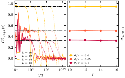
Figure 2: Left panel. Correlation function $C_{L/2+1}^{\theta}\left(t\right)$ as a function of time for a number of system sizes (varying line style) and perturbation strengths (varying color intensity, see legends). The dashed dotted black lines correspond to $\Delta_{L/2+1}$, the height of the intermediate plateau . Right panel. The height of the intermediate plateau, $\Delta_{L/2+1}=2^{-L}\sum_{\alpha}\max_{\beta}\left|\left\langle\alpha\left|\hat{Z}_{L/2+1}\right|\beta\right\rangle\right|^{2}$, as a function of the system size, for a number of perturbations strengths (see legend). The rest of the parameters used in the calculation are $h=0.5$, $J_{0}=1$, $J_{\gamma}=3$, $V=0.5$ and $T=1$.

Localization.—The model with $V=h=\theta=0$ has trivially localized domain-walls (DWs). In what follows we show that localization remains robust, as long as the interaction $J_{i}$ is unbounded. We will only consider the stability for $\theta=0$, the stability for $\theta\neq 0$ follows from general arguments of stability of Floquet-MBL. We write the total Hamiltonian $\hat{H}_{I}$ as $\hat{H}_{I}=\hat{H}_{0}+\hat{H}_{h}+\hat{H}_{V}$, where $\hat{H}_{h,V}$ are the two off-diagonal terms in Eq. (5). An eigenstate of $\hat{H}_{0}$ with $n$ DWs at positions $i_{1},\ldots i_{n}$ has energy $E_{\left\{i_{m}\right\}}=\sum_{j}J_{j}-2\sum_{i\in\left\{i_{m}\right\}}J_{i}$. Both of $\hat{H}_{h}$ and $\hat{H}_{V}$ only connect it to states with $n,n\pm 2$ DWs . Adding or removing a DW at $i$ changes $E_{\left\{i_{m}\right\}}$ by $\pm 2J_{i}$, while moving a DW from $i$ to $i+r$, changes the energy by $2\left(J_{i}-J_{i+r}\right)$. Restricting our discussion to $\hat{H}_{h}$ for simplicity (the discussion for $\hat{H}_{V}$ is almost identical), we note that given an eigenstate of $\hat{H}_{0}$ with $n$ DWs, the states closest in energy connected to it by leading-order perturbation theory also have $n$ DWs, with a single DW moved by one site. Restricting the Hamiltonian to single domain-wall states, valid for small $h$ (see Sup. Mat.  for more details), and writing $\left|i\right\rangle$ for a state with a single domain wall at $i$, gives the effective single-particle Hamiltonian

$$\left\langle i\right|\hat{H}\left|j\right\rangle=2J_{j}\delta_{i,j}+h\left(\delta_{i,j+1}+\delta_{i,j-1}\right),$$ (6)

so that a DW behaves like a single particle hopping around with a uniform hopping amplitude $h$ and potential $J_{j}$. For a linear $J_{i}=J_{0}+J_{\gamma}\left(i-\frac{L}{2}\right)$ the problem reduces to Stark localization [24, 25]. Localization persists for states with multiple DWs (see Supp. Mat. for more information).

Correlation function.—The combination of localization and quasi-degeneracy leads to each eigenstate $\left|\alpha\right\rangle$ having a partner eigenstate $\left|\bar{\alpha}\right\rangle$ lying within a quasi-energy window $\Delta E=O\left(e^{-L}\right)$ and having an off-diagonal matrix element $\left|\left\langle\alpha\left|\hat{Z}_{i}\right|\bar{\alpha}\right\rangle\right|^{2}$ remaining finite even in the TDL. In this case, the correlation function, $C_{i}^{\theta}$, will have an intermediate plateau of height $\Delta_{i}=2^{-L}\sum_{\alpha}\left|\left\langle\alpha\left|\hat{Z}_{i}\right|\bar{\alpha}\right\rangle\right|^{2}$ for times up to $t_{*}\sim\exp\left(L\right)$ as discussed earlier; after this time, the correlation function decays. This is shown in the left panel of Fig. 2 where we numerically compute $C_{L/2+1}^{\theta}$ for a number of $\theta$ and system sizes. The left panel shows that $C_{L/2+1}^{\theta}$ displays an intermediate plateau persisting for times exponentially large in system size before decaying and fluctuating around zero. In the right panel of Fig. 2, we calculate $\Delta_{L/2+1}$ as follows: for each eigenstate $\left|\alpha\right\rangle$ of $\hat{U}_{\theta}\left(T\right)$ we take the 10 closest (in quasi-energy) $\left|\beta\right\rangle$, and compute $\Delta_{L/2+1}=2^{-L}\sum_{\alpha}\max_{\beta}\left|\left\langle\alpha\left|\hat{Z}_{L/2+1}\right|\beta\right\rangle\right|^{2}$. The dash-dotted lines in the left panel show that the $\Delta_{L/2+1}$ obtained quantitatively reproduces the height of the intermediate plateau, while the right panel shows that this height doesn’t decay with system size for a range of perturbations $\theta$.

We now turn to the fluctuations of $C_{i}^{\theta}\left(t\right)$ around the intermediate plateau, showing that they vanish in the thermodynamic limit: $\lim_{t\to\infty}\lim_{L\to\infty}C_{i}^{\theta}\left(t\right)=c>0$.

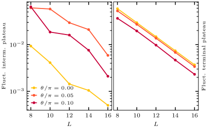
Figure 3: Temporal fluctuations of the correlation function $C_{L/2+1}^{\theta}\left(t\right)$ around the intermediate plateau (left) and the terminal plateau (right) as a function of the system size and perturbation strength $\theta$. The rest of the parameters used in the calculation are $h=0.5$, $J_{0}=1$, $J_{\gamma}=3$, $V=0.5$ and $T=1$.

Fluctuations.—The magnitude of the temporal fluctuations in the terminal plateau can be calculated by infinite-time average of $\left|C_{\theta}\left(t\right)\right|^{2}$ and is given by $2^{-L}\sum_{\alpha,\beta}\left|\left\langle\alpha\left|\hat{Z}_{i}\right|\beta\right\rangle\right|^{4}$. As discussed bellow Eq. (2) it decays exponentially with $L$, as we indeed see in the right panel of Fig. 3. To compute the temporal fluctuations around the intermediate plateau, we compute the time-average up-to time $t_{*}$ which we explicitly set as the departure time from the intermediate plateau. For all studied values of parameters the fluctuations decay with system size. Combined with the fact that $t_{*}\sim\exp\left(L\right)$, this suggests that $\lim_{t\to\infty}\lim_{L\to\infty}C_{i}^{\theta}\left(t\right)=c>0$, namely there exists a stable non-ergodic liquid phase. Adding a spin-flipping operator $\hat{P}$ every period, the non-ergodic time-liquid is readily modified into a DTC, and shows subharmonic oscillations for sufficiently large $J$ (see Fig. 1).

Conclusions.–In conclusion, we have presented a detailed study of DTCs in a class of non-disordered, non-integrable Ising-type systems. We discuss a general mechanism, which relies on localisation and quasi-degeneracy. We then present approximate analytical arguments that our models do have these properties, with localisation relying on Stark-type physics of domain walls and perturbatively stable degeneracy lifted by finite-size effects resulting in finite lifetime of the DTC for finite-sized systems. We finally numerically demonstrate these results. Thus overall there is DTC order in the thermodynamic limit, but the limits of long time and large size do not commute. This is again a telltale sign that the mechanism we discuss is at play, as the finite-size lifting of the degeneracy is the root cause of the finite lifetimes. While in this work we have focused only on linear potentials, our arguments readily generalize to other unbounded potentials.

Our class of models is disorder-free, unitary, many-body, and display DTC with exponentially-long lifetimes. Experimental demonstration of our results requires similar machinery as that of disordered DTCs [5, 19] and so should be within reach of current setups.

References

- Watanabe and Oshikawa [2015] H. Watanabe and M. Oshikawa, Absence of Quantum Time Crystals, Phys. Rev. Lett. 114, 251603 (2015).
- Lazarides et al. [2015] A. Lazarides, A. Das, and R. Moessner, Fate of many-body localization under periodic driving, Phys. Rev. Lett. 115, 30402 (2015).
- Ponte et al. [2015a] P. Ponte, A. Chandran, Z. Papić, and D. A. Abanin, Periodically driven ergodic and many-body localized quantum systems, Ann. Phys. (N. Y). 353, 196 (2015a).
- D’Alessio and Rigol [2014] L. D’Alessio and M. Rigol, Long-time behavior of isolated periodically driven interacting lattice systems, Phys. Rev. X 4, 41048 (2014).
- Khemani et al. [2016] V. Khemani, A. Lazarides, R. Moessner, and S. L. Sondhi, Phase structure of driven quantum systems, Phys. Rev. Lett. 116, 250401 (2016).
- Berges et al. [2004] J. Berges, S. Borsányi, and C. Wetterich, Prethermalization., Phys Rev Lett 93, 142002 (2004).
- Mori et al. [2017] T. Mori, T. N. Ikeda, E. Kaminishi, and M. Ueda, Thermalization and prethermalization in isolated quantum systems: a theoretical overview, arXivJ. Phys. B 51, 112001 (2018) , 1712.08790v2 (2017).
- Abanin et al. [2015] D. Abanin, W. D. Roeck, W. W. Ho, and F. Huveneers, A rigorous theory of many-body prethermalization for periodically driven and closed quantum systems, Commun. Math. Phys. 354, 809-827 (2017) , 1509.05386v3 (2015).
- Else et al. [2017] D. V. Else, B. Bauer, and C. Nayak, Prethermal phases of matter protected by time-translation symmetry, Physical Review X 7 (2017).
- Abanin et al. [2019] D. A. Abanin, E. Altman, I. Bloch, and M. Serbyn, Colloquium: Many-body localization, thermalization, and entanglement, Reviews of Modern Physics 91, 021001 (2019).
- Nandkishore and Huse [2014] R. Nandkishore and D. A. Huse, Many body localization and thermalization in quantum statistical mechanics, Annual Review of Condensed Matter Physics, Vol. 6: 15-38 (2015) , 1404.0686v2 (2014).
- Ponte et al. [2015b] P. Ponte, Z. Papić, F. Huveneers, and D. A. Abanin, Many-body localization in periodically driven systems, Phys. Rev. Lett. 114, 140401 (2015b).
- Rehn et al. [2016] J. Rehn, A. Lazarides, F. Pollmann, and R. Moessner, How periodic driving heats a disordered quantum spin chain, Phys. Rev. B 94, 020201 (2016).
- Else et al. [2016] D. V. Else, B. Bauer, and C. Nayak, Floquet time crystals, Phys. Rev. Lett. 117, 090402 (2016).
- Yao et al. [2017] N. Y. Yao, A. C. Potter, I. D. Potirniche, and A. Vishwanath, Discrete time crystals: Rigidity, criticality, and realizations, Phys. Rev. Lett. 118, 030401 (2017).
- Zhang et al. [2017] J. Zhang, P. W. Hess, A. Kyprianidis, P. Becker, A. Lee, J. Smith, G. Pagano, I. D. Potirniche, A. C. Potter, A. Vishwanath, N. Y. Yao, and C. Monroe, Observation of a discrete time crystal, Nature 543, 217 (2017).
- Choi et al. [2017] S. Choi, J. Choi, R. Landig, G. Kucsko, H. Zhou, J. Isoya, F. Jelezko, S. Onoda, H. Sumiya, V. Khemani, C. von Keyserlingk, N. Y. Yao, E. Demler, and M. D. Lukin, Observation of discrete time-crystalline order in a disordered dipolar many-body system, Nature 543, 221 (2017).
- Ho et al. [2017] W. W. Ho, S. Choi, M. D. Lukin, and D. A. Abanin, Critical time crystals in dipolar systems, Phys. Rev. Lett. 119, 010602 (2017).
- Mi et al. [2022] X. Mi et al., Time-crystalline eigenstate order on a quantum processor, Nature 601, 531 (2022).
- Pal et al. [2018] S. Pal, N. Nishad, T. S. Mahesh, and G. J. Sreejith, Temporal order in periodically driven spins in star-shaped clusters, Phys. Rev. Lett. 120, 180602 (2018).
- Schulz et al. [2019] M. Schulz, C. Hooley, R. Moessner, and F. Pollmann, Stark many-body localization, Physical review letters 122, 040606 (2019).
- van Nieuwenburg et al. [2019] E. van Nieuwenburg, Y. Baum, and G. Refael, From bloch oscillations to many-body localization in clean interacting systems, Proceedings of the National Academy of Sciences 116, 9269 (2019).
- Ribeiro et al. [2020] P. Ribeiro, A. Lazarides, and M. Haque, Many-body quantum dynamics of initially trapped systems due to a stark potential: Thermalization versus bloch oscillations., Phys Rev Lett 124, 110603 (2020).
- Zener [1934] C. Zener, A theory of the electrical breakdown of solid dielectrics, Proc. R. Soc. A 145, 523 (1934).
- Wannier [1960] G. H. Wannier, Wave Functions and Effective Hamiltonian for Bloch Electrons in an Electric Field, Phys. Rev. 117, 432 (1960).
- Zisling et al. [2022] G. Zisling, D. M. Kennes, and Y. Bar Lev, Transport in Stark many-body localized systems, Phys. Rev. B 105, L140201 (2022).
- [27] B. Kloss, J. C. Halimeh, A. Lazarides, and Y. Bar Lev, Absence of localization in interacting spin chains with a discrete symmetry, Nature Communications 14, 3778.
- Bhakuni et al. [2020] D. S. Bhakuni, R. Nehra, and A. Sharma, Drive-induced many-body localization and coherent destruction of stark many-body localization, Physical Review B 102 (2020).
- Deger et al. [2023] A. Deger, C. Duffin, and A. Lazarides, Driven interacting stark system, in preparation (2023).
- Kshetrimayum et al. [2020] A. Kshetrimayum, J. Eisert, and D. M. Kennes, Stark time crystals: Symmetry breaking in space and time, Phys. Rev. B 102, 195116 (2020) , 2007.13820v2 (2020).
- Liu et al. [2023] S. Liu, S. Zhang, C. Hsieh, S. Zhang, and H. Yao, Discrete time crystal enabled by stark many-body localization., Phys Rev Lett 130, 120403 (2023).
- Reimann [2008] P. Reimann, Foundation of statistical mechanics under experimentally realistic conditions, Phys. Rev. Lett. 101, 190403 (2008).
- Linden et al. [2009] N. Linden, S. Popescu, A. J. Short, and A. Winter, Quantum mechanical evolution towards thermal equilibrium, Phys. Rev. E 79, 61103 (2009).
- Russomanno et al. [2012] A. Russomanno, A. Silva, and G. E. Santoro, Periodic steady regime and interference in a periodically driven quantum system, Phys. Rev. Lett. 109, 257201 (2012).
- Lazarides et al. [2014a] A. Lazarides, A. Das, and R. Moessner, Periodic thermodynamics of isolated quantum systems, Phys. Rev. Lett. 112, 150401 (2014a).
- Lazarides et al. [2014b] A. Lazarides, A. Das, and R. Moessner, Equilibrium states of generic quantum systems subject to periodic driving, Phys. Rev. E 90, 12110 (2014b).
- Note [1] It is easy to construct non-local observables, with arbitrary long-time dependence.
- Note [2] Similarly to a liquid which is invariant to spatial translations.
- Note [3] Note that the observable will generically change within the period.
- Note [4] For static systems this is the Hamiltonian, , while for periodically driven systems it is the effective Hamiltonian, , where is the one period unitary propagator.
- Alhambra et al. [2020] Á. M. Alhambra, J. Riddell, and L. P. García-Pintos, Time Evolution of Correlation Functions in Quantum Many-Body Systems, Phys. Rev. Lett. 124, 110605 (2020).
- Lezama et al. [2023] T. L. M. Lezama, Y. Bar Lev, and L. F. Santos, Temporal fluctuations of correlators in integrable and chaotic quantum systems (2023), arXiv:2307.08440 [cond-mat.str-el] .
- Note [5] Since the condition is on energy gaps, the arbitrariness in the definition of is insignificant.
- Note [6] For Floquet systems the infinite time average should be correspondingly adjusted.
- Serbyn et al. [2014] M. Serbyn, Z. Papić, and D. A. Abanin, Quantum quenches in the many-body localized phase, Phys. Rev. B 90, 174302 (2014).
- Khemani et al. [2017] V. Khemani, C. W. von Keyserlingk, and S. L. Sondhi, Defining time crystals via representation theory, Phys. Rev. B 96, 115127 (2017).
- Note [7] This is true as long as the spectrum of and has non-degenerate gaps, which is true in general for a finite system. In addition the spectrum is non-degenerate as we require stability to local periodic perturbations.
- Note [8] The diagonal terms are excluded from the sum because when the eigenstates of are non-degenerate they are also eigenstates of , and such that .
- Note [9] For example, the eigenstates of the disordered Ising model, , are trivially localized, but eigenstates for which is finite are at least apart in energy.
- Huse et al. [2013] D. A. Huse, R. Nandkishore, V. Oganesyan, A. Pal, and S. L. Sondhi, Localization protected quantum order, Phys. Rev. B 88, 14206 (2013).
- Note [10] Except when acting at the edges of the system when they may also connect to states with .
- Note [11] For , there are two degenerate states with the domain wall at . One can label them with an internal pseudospin degree of freedom, and the Hamiltonian in Eq. 6 would then not mix the two. We omit this here for notational simplicity.