Random Generation of Git Graphs

Abstract

Version Control Systems, such as Git and Mercurial, manage the history of a project as a Directed Acyclic Graph encoding the various divergences and synchronizations happening in its life cycle. A popular workflow in the industry, called the feature branch workflow, constrains these graphs to be of a particular shape: a unique main branch, and non-interfering feature branches.

Here we focus on the uniform random generation of those graphs with $n$ vertices, including $k$ on the main branch, for which we provide three algorithms, for three different use-cases. The first, based on rejection, is efficient when aiming for small values of $k$ (more precisely whenever $k=O(\sqrt{n})$). The second takes as input any number $k$ of commits in the main branch, but requires costly precalculation. The last one is a Boltzmann generator and enables us to generate very large graphs while targeting a constant $k/n$ ratio. All these algorithms are linear in the size of their outputs.

1 Motivation

In software development, Version Control Systems (VCS in short) such as Git or Mercurial are crucial. They facilitate collaborative work by allowing multiple developers to concurrently contribute to a shared file system. VCS automatically save all project versions over time, along with the associated changes.

Most VCS offer branching support, allowing developers to diverge from the main line of development and continue their work independently without affecting the main project line. These branches can be subsequently merged, in order to integrate changes from one branch into another, like new features or bug fixes.

In the abstract, the history of a VCS repository can be seen as a Directed Acyclic Graph (DAG), where vertices are the different versions of the project (also named commits) and arcs symbolize the changes between two versions. There are no restrictions on the shape of the graphs you can generate with a VCS, but many projects follow a workflow, that is a process and a set of conventions that define how branches are created, and how changes are integrated into the main codebase.

The purpose of this paper is to develop an efficient random sampler for DAGs that respect a particular workflow.

One benefit of such a sampler would be to integrate property-based tests into VCS development. In these tests, instead of specifying explicit input values and expected outcomes, we define properties that should be satisfied for a wide range of repositories, which are generated randomly during the test. By generating diverse graph structures that adhere to the workflow’s specifications, we ensure a comprehensive examination of the VCS’s behavior according to plausible scenarios. To give a concrete example based on work by one of the authors [CDL23], a random DAG sampler could experimentally check the effectiveness of git bisect, an algorithm that finds the commit where a bug has been introduced.

In this paper, we will take a look at one of the simplest workflows, but one that is widely used in the corporate world: the feature branch workflow. In this workflow, the non-main branches do not interfere with each other, and are simply attached to the (unique) main branch. Here is a more formal definition of graphs induced by this workflow. (This definition originally comes from [Lec24].)

Definition 1 (Git graph).

A Git feature branch graph (or just Git graph) is a DAG that consists of:

• a main branch, that is a directed path of black vertices.

• potentially several feature branches, that are directed paths that start and end on vertices of the main branch. The set of intermediary vertices is not empty and consists of white vertices. A black vertex cannot be the end point of several feature branches, just one at most (but it can be the starting point of several branches).

Figure 1: All Git graphs with $5$ vertices including $3$ black vertices. Edges are oriented from left to right. Free vertices are outlined in orange.

The size of a Git graph $\gamma$ is its number of vertices. By convention, we assume that there exists a unique Git graph of size $0$. Another important parameter is its number of black vertices, and will be denoted by $k(\gamma)$. A black vertex is said to be free if there is no feature branch ending on it, i.e. its indegree is at most $1$. All Git graphs $\gamma$ of size $5$ with $k(\gamma)=3$ are listed in Figure 1.

The fact that we forbid merges of multiple feature branches into the main one is not a restriction of the VCS, but is advisable to maintain a clearer and more understandable project history, reduce the risk of conflicts, and enhance traceability and maintainability. This restriction is also discussed in [CDL23].

2 The uniform model

2.1 A recursive decomposition

We first describe a recursive decomposition of Git graphs, based on the number of black vertices. Consider the last black vertex $v_{k}$ of a Git graph of size $n$ and with $k>1$ black vertices. There are only two possibilities: either $v_{k}$ is free, or $v_{k}$ is a merge between the main branch and a feature branch (which is unique, by definition). In the latter case, the feature branch starts with a black vertex, which can be any vertex of the main branch, but $v_{k}$. Removing $v_{k}$ and the potential feature branch attached to it leads to a smaller Git graph.

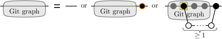
Figure 2: How to decompose a Git graph.

By this reasoning, illustrated by Figure 2, we obtain the induction formula

$$g_{n,k}=g_{n-1,k-1}+\sum_{\ell\geq 0}(k-1)g_{n-1-\ell,k-1},\quad\text{with }g_{0,k}=\begin{cases}1&\text{if }k=0\\ 0&\textrm{otherwise}\end{cases}$$ (1)

where $g_{n,k}$ is the number of Git graphs with $n$ vertices, $k$ of them being black.

This induction is sufficient to write a recursive generator (see [NW78] for the general theory of recursive samplers and [FZV94] for a more modern point of view in the context of the symbolic method). We do not extend on this generator as we will show in Section 2.2 that it always yields similar objects. Moreover, recursive samplers generally suffer from the high cost of precomputing the large numbers $g_{n,k}$ which makes then impractical for large values of $n$.

It is straightforward (especially if you are familiar with the symbolic method [FS09]) to translate Formula (1) into a differential equation whose solution is the generating function $G(z,u)$ of Git graphs:

$$G(z,u)=1+zuG(z,u)+\frac{z^{2}u^{2}}{1-z}\frac{\partial G}{\partial u}(z,u),\quad\text{where~{}}G(z,u)\coloneqq\sum_{n\geq 0}\sum_{k\geq 0}g_{n,k}z^{n}u^{k}.$$ (2)

Note that $G(z,u)$ is not analytic at $z=0$ since the number of Git graphs grows as a factorial (we have $g_{2k-1,k}\geq(k-1){!}$ by considering a Git graph with only merge commits and feature branches of length $1$). For this reason, the previous equation does not seem to be usable for Boltzmann sampling.

2.2 Most Git graphs look alike under the uniform distribution

A large random Git graph is with high probability of the same shape: about half of the commits are on the main branch, and most commits on the main branch are merges of size-$1$ branches.

Proposition 1.

Let $u$ be any real positive number. Consider $\gamma_{n}$ a random Git graph of size $n$ taken with probability $\dfrac{u^{k(\gamma_{n})}}{\sum_{\gamma\text{ Git graph\ of size }n}u^{k(\gamma)}}$. Then the random variable $\frac{k(\gamma_{n})}{n}$ converges in probability to $\frac{1}{2}$ when $n$ goes to $+\infty$. (Note that $u=1$ corresponds to the uniform distribution).

The intuition behind this result is a large number of branches greatly increases the number of ways of connecting them to the main branch, hence favoring graphs with many short branches over ones with fewer but longer branches.

In particular, for any value of $u$, the average number of commits in the main branch is asymptotically equivalent to $\frac{n}{2}$. This motivates the introduction of a variant of this model which we detail in the next half of this paper, and which allows more control over the number of commits on the main branch.

2.3 A rejection algorithm

Before delving into the next model, it is worth noting that there is an efficient rejection-based sampling algorithm for the case where $k$ is small based on the following inclusion. Consider a variation $\mathcal{H}$ of the model where every black vertex but the first one is the endpoint of a feature branch but it is allowed to have zero commit on a feature branch. Denote by $h_{n,k}$ the number of such graphs with $n$ vertices including $k$ on the main branch. Then Git graphs can be seen as a subset of these graphs by identifying empty feature branches pointing at the root commit in $\mathcal{H}$ with free commits in Git graphs. Moreover, whenever $k\leq t\sqrt{n}$, for some constant $t>0$, we have that

$$g_{n,k}=\Theta(h_{n,k})\quad\text{where the bounds depend only on~{}$t$}.$$

This yields Algorithm 1 for sampling uniform Git graphs with a small main branch. This algorithm can be implemented so as to perform $O(k)$ array accesses and $O(k)$ RNG calls in average.

Algorithm 1 Rejection algorithm for Git graphs with $n$ vertices, $k$ of them being black

1:start with a chain of $k$ black vertices

2:arrange uniformly at random $(n-k)$ white vertices into $(k-1)$ possibly empty chains

3:attach the ends of these chains to the $(k-1)$ last black vertices

4:attach the start of every chain to a previous black vertex, chosen uniformly at random

5:if any of the empty chains is not attached to the root, start over, otherwise return

3 The labeled-main distribution

3.1 Description of the model

Given the disadvantages of the uniform distribution, we propose a new model for random Git graphs that is easier to sample, gives with more varied shapes, and with fine control over the number of black vertices. The principle is that a Git graph $\gamma$ will have a probability to be generated proportional to $u^{k(\gamma)}/{k(\gamma)}{!}$ where $u$ is a real positive parameter.

More precisely, we set $\widetilde{G_{n}}(u):=\sum_{k=1}^{n}g_{n,k}\frac{u^{k}}{k!}$ and $\widetilde{G}(z,u):=\sum_{n\geq 0}\widetilde{G_{n}}(u)z^{n}$. Thus $\widetilde{G}$ resembles an exponential generating function, but with a scaling of $k{!}$ instead of a scaling of $n{!}$. Unlike $G$ defined in the previous section, the function $\widetilde{G}$ is analytic at $z=0$ (a direct consequence of Theorem 1 below).

Definition 2.

The probability under the labeled-main distribution of a Git graph of size $n$ and with $k$ black vertices is defined as $\frac{u^{k}z^{n}}{k!\widetilde{G}(z,u)}$, where $z$ and $u$ are positive parameters inside the domain of convergence of $\widetilde{G}$.

This is a multivariate Boltzmann model (exponential in $u$ and ordinary in $z$). A sampler based on this distribution falls into the category of Boltzmann generators, for which a large number of results have been established, facilitating the generation of large objects [DFLS04].

By using the Borel transform [Bor99] on Equation (2) with respect to the variable $u$, that is to say $\sum_{n,k\geq 0}a_{n,k}z^{n}u^{k}\mapsto\sum_{n,k\geq 0}\frac{a_{n,k}z^{n}u^{k}}{k!}$, we can obtain a differential equation for $\widetilde{G}(z,u)$:

$$\frac{\partial\widetilde{G}}{\partial u}(z,u)=z\widetilde{G}(z,u)+\frac{z^{2}u}{1-z}\frac{\partial\widetilde{G}}{\partial u}(z,u)\qquad\text{and}\qquad\widetilde{G}(z,0)=1.$$ (3)

Solving this differential equation gives a nice formula for $\widetilde{G}$.

Theorem 1.

The function $\widetilde{G}(z,u)=\sum_{n\geq 0}\sum_{k=1}^{n}g_{n,k}\frac{u^{k}}{k!}$ is equal to

$$\widetilde{G}(z,u)={\left(1-\frac{z^{2}u}{1-z}\right)}^{-\frac{1-z}{z}}.$$

By a tedious but straightforward application of the transfer theorem [FS09], we can compute the average number of black vertices under the labeled-main  distribution.

Proposition 2.

Let $k(\gamma_{n})$ be the number of commits in the main branch of a graph $\gamma_{n}$ taken at random with probability $\mathbb{P}(\gamma_{n})=\frac{u^{k(\gamma_{n})}}{k(\gamma_{n})!}\frac{1}{\widetilde{G_{n}}(u)}$. The mean and variance of $k(\gamma_{n})$ are asymptotically equivalent to

$$\mathbb{E}(k(\gamma_{n}))\sim\frac{1-\rho_{u}}{2-\rho_{u}}n\quad\text{ and }\quad\mathbb{V}(k(\gamma_{n}))\sim\frac{\rho_{u}(1-\rho_{u})}{{(2-\rho_{u})}^{3}}n,\quad\text{ where }\rho_{u}=\frac{\sqrt{1+4u}-1}{2u}.$$

Remark that the expected value of the $k(\gamma)/n$ ratio can be any number between $0$ and $1/2$, depending on the value of $u$. This is one of the main benefits of the labeled-main distribution: given any $\alpha\in(0,\frac{1}{2})$, we can tune $u$ in order to target Git graphs to have $\alpha n$ black vertices (and the variance is quite tight).

3.2 A bijection with cyclariums

The closed formula for $\widetilde{G}$ featured in Theorem 1 calls for a combinatorial interpretation. That is why we define a new family of combinatorial objects: the cyclariums.

A cyclarium is defined as a set of cycles of $k$ black vertices labeled by $\{1,\dots,k\}$ where each vertex that has not the largest label inside its own cycle carries a non-empty chain of white vertices. See Figure 3 top left to see an illustration of a cyclarium. The set $\mathcal{Y}$ of cyclariums has the natural combinatorial specification

$$\mathcal{Y}=\textsc{Set}\left(\mathcal{C}\right),\quad\textsc{Seq}_{\neq 0}\left(\mathcal{Z}\right)\times\mathcal{C}=\textsc{Cyc}\left(\mathcal{U}\mathcal{Z}\textsc{Seq}_{\neq 0}\left(\mathcal{Z}\right)\right)$$ (4)

where $\textsc{Set}\left(\cdot\right)$, $\textsc{Seq}_{\neq 0}\left(\cdot\right)$ and $\textsc{Cyc}\left(\cdot\right)$ are respectively the operators for sets, non-empty sequences and cycles. Consequently the generating function of cyclariums (scaled by $k{!}$) is also given by the formula of Theorem 1 (for more details on the symbolic method, see [FS09]).

Proposition 3.

The Git graphs with $n$ vertices, $k$ black vertices and $f$ free vertices are in bijection with the cyclariums with $n$ vertices, $k$ black vertices and $f$ cycles.

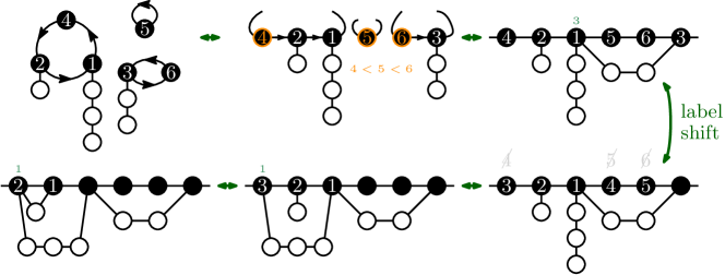
Figure 3: Outline of the bijection between Git graphs and cyclariums

The bijection is depicted in Figure 3. We give a quick overview of the transformation from cyclariums to Git graphs. First, we break each cycle just before the vertex with the largest label, so that they are directed paths. Then we sort these paths according to their largest label, and concatenate them. Now we process the black vertices from right to left. If a chain of white vertices is attached to the current black vertex $\boldsymbol{v}$, then we connect this chain to the black vertex whose position is given by the label of $\boldsymbol{v}$. If no chain is attached, we do nothing. Once the vertex has been processed, its label $\ell$ is deleted and we change all labels $x$ such that $x>\ell$ by $x-1$. We can check that we eventually obtain a Git graph.

Exploiting the fact that the permutations with $f$ cycles are counted by the Stirling numbers of the first kind, we obtain a closed formula for $g_{n,k}$.

Corollary 1.

The number of Git graphs $g_{n,k}$ of size $n$ and with $k$ black vertices is $1$ if $k=n$ and

$$g_{n,k}=\sum_{f=1}^{k-1}{k\brack f}{n-k-1\choose k-f-1}$$

for $k<n$, where ${\cdot\brack\cdot}$ denotes the (unsigned) Stirling number of the first kind.

The bijection also suggests a sampling algorithm for Git graphs of size $n$ if we fix the number $k$ of black vertices and optionally the number $f$ of free vertices: see Algorithm 2. It runs in $O(n)$ (with some optimization) but requires an expensive precomputation of the Stirling numbers of the first kind. This precomputation is in particular used to generate a uniform permutation of size $k$ with $f$ cycles. If $f$ must be sampled, we need to precompute $O(k^{2})$ numbers of size $O(k\log k)$. If $f$ is given, only $O(f(k-f))$ of them can be precalculated.

Algorithm 2 Exact sampler of Git graphs with $n$ vertices and $k$ black vertices

1:$f$, the number of free vertices

2:If $f$ is not given, sample it with probability ${k\brack f}{n-k-1\choose k-f-1}/g_{n,k}$

3:Generate a random permutation of size $k$ with $f$ cycles

4:Generate a composition of $n-k$ into $k-f$ positive terms

5:Form $k-f$ chains of white vertices whose lengths are given by the previous composition

6:Attach them to the permutation to form a cyclarium

7:Use the bijection from cyclariums to Git graphs

3.3 A Boltzmann generator

Specification (4) induces a natural Boltzmann generator [DFLS04] for cyclariums, and hence by Proposition 3 a Boltzmann generator for Git graphs under the labeled-main distribution. Rather than simply generating a cyclarium of size $n$ and applying the bijection, which would result in $O(n^{2})$ complexity, we can mix the two approaches and achieve $O(n+f^{2})$ complexity, where $f$ is the number of free vertices (which is logarithmic in $n$ in average). The details are given in Algorithm 3 and illustrated by Figure 4.

Algorithm 3 Boltzmann sampler under the labeled-main distribution of parameters $z$ and $u$

1:$f\leftarrow\text{{Poisson}($\ln\tilde{G}(z,u)$)}$$\triangleright$ Poisson distribution

2:cycle_lengths $\leftarrow$ array of $f$ independent Loga($\frac{uz^{2}}{1-z}$) $\triangleright$ Logarithmic series distribution

3:$k\leftarrow$ total sum of cycle_lengths

4:$g\leftarrow$ directed path of $k$ black vertices denoted $v[0],\dots,v[{k-1}]$ $\triangleright$ skeleton of our Git graph

5:while  $k>0$  do

6:      extract a number $x$ from cycle_lengths with probability $x/k$

7:      mark $v[{k-x}]$

8:      $k\leftarrow k-x$

9:for $j$ from $1$ to number of black vertices $-1$ do

10:     if $v[j]$ is not marked then

11:         $i\leftarrow$ random number between $0$ and $j-1$

12:         link $v[i]$ to a directed path of $(1+\text{{Geom}($z$)})$ white vertices$\triangleright$ Geometric distribution

13:         link the last vertex of this path to $v[j]$      

14:return $g$

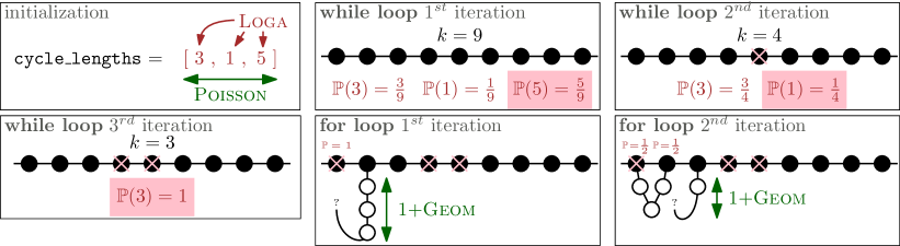
Figure 4: Illustration of the first steps of Algorithm 3.

Our implementation of this algorithm in Python easily generates graphs larger than 10 million. We also recall that we can carefully choose the parameters $z$ and $u$ to target a size $n$ and a ratio $\alpha\in(0,\frac{1}{2})$, where $\alpha n$ is the number of black vertices.

4 Conclusion

In this work, we have developed three random generators for Git graphs. The Python source code for these algorithms is enclosed with this submission.

A few questions remain unanswered. Firstly, our algorithms are unable to generate graphs for certain values of $k$ efficiently (more precisely when $k$ is in the window $\sqrt{n}\ll k\ll n$, and when $k\geq\frac{n}{2}$). In addition, it would be interesting to obtain an asymptotic estimate of the numbers $g_{n}$ of Git graphs. The formula in Corollary 1 seems to be a good start to do so. Moreover, we could study potential phase transitions as $k$ evolves as a function of $n$. In particular, we could investigate how the number of free vertices grows, as well as the gaps between each of them.

Finally, we could study more involved workflows, and enumerate DAGs that adhere to them.

References

- [Bor99] Émile Borel “Mémoire sur les séries divergentes” In Annales scientifiques de l’École Normale Supérieure 3e série, 16 Elsevier, 1899, pp. 9–131 DOI: 10.24033/asens.463
- [CDL23] Julien Courtiel, Paul Dorbec and Romain Lecoq “Theoretical Analysis of Git Bisect” In Algorithmica, 2023 DOI: 10.1007/s00453-023-01194-0
- [DFLS04] Philippe Duchon, Philippe Flajolet, Guy Louchard and Gilles Schaeffer “Boltzmann samplers for the random generation of combinatorial structures” In Combinatorics, Probability & Computing 13.4-5 Cambridge University Press, 2004, pp. 577–625 DOI: 10.1017/S0963548304006315
- [FS09] Philippe Flajolet and Robert Sedgewick “Analytic Combinatorics” Cambridge University Press, 2009, pp. I–XIII\bibrangessep1–810
- [FZV94] Philippe Flajolet, Paul Zimmermann and Bernard Van Cutsem “A calculus for the random generation of labelled combinatorial structures” In Theoretical Computer Science 132.1-2 Elsevier, 1994, pp. 1–35
- [Lec24] Romain Lecoq “Analyse de git bisect et problème de propagation (temporary title)” in French, work in progress, 2024
- [NW78] Albert Nijenhuis and Herbert Wilf “Combinatorial Algorithms: For Computers and Hard Calculators” USA: Academic Press, Inc., 1978
- [Pit06] J. Pitman “Combinatorial stochastic processes” Lectures from the 32nd Summer School on Probability Theory held in Saint-Flour, July 7–24, 2002, With a foreword by Jean Picard 1875, Lecture Notes in Mathematics Springer-Verlag, Berlin, 2006, pp. x+256
- [Wil99] Herbert S. Wilf “East Side, West Side . . . - an introduction to combinatorial families-with Maple programming”, 1999 URL: https://www2.math.upenn.edu/~wilf/eastwest.pdf