Robustness bounds on the successful adversarial examples: Theory and Practice

Abstract

Adversarial example (AE) is an attack method for machine learning, which is crafted by adding imperceptible perturbation to the data inducing misclassification. In the current paper, we investigated the upper bound of the probability of successful AEs based on the Gaussian Process (GP) classification. We proved a new upper bound that depends on AE’s perturbation norm, the kernel function used in GP, and the distance of the closest pair with different labels in the training dataset. Surprisingly, the upper bound is determined regardless of the distribution of the sample dataset. We showed that our theoretical result was confirmed through the experiment using ImageNet. In addition, we showed that changing the parameters of the kernel function induces a change of the upper bound of the probability of successful AEs.

Keywords Gaussian Processes, Adversarial Examples, Theoretical Bound

1 Introduction

1.1 Adversarial example

Nowadays, machine learning is widely used in various fields, and concern about its security has emerged. Among such attack methods, an adversarial example (AE) is widely known  [goodfellow_explaining_2015]. AE is the sample that is different slightly from the natural sample that is misclassified by a machine learning classifier [goodfellow_explaining_2015]. AE is often crafted against neural networks by adding a small perturbation (adversarial perturbation) to the original input, and various methods for crafting adversarial perturbation are proposed  [goodfellow_explaining_2015, carlini_towards_2017].

Since AE is regarded as an attack method against machine learning, various defense methods against AE have been investigated, including the detection method [feinman_detecting_2017], and adversarial training  [cai_curriculum_2018] However, Carlini & Wagner [carlini_adversarial_2017] reviewed ten detection methods, and stated that no defense method could survive a white-box AE attack, an attack using the knowledge of the victim’s architecture. Therefore, not only the separate defense methods but also the theoretical basis of AE should be required for the defense against AE.

In the current study, we investigated the theoretical basis of AE using the Gaussian Process (GP). GP is a stochastic process whose output is distributed according to the Gaussian distribution. GP can be used for classification and regression [rasmussen_gaussian_2006], and previous research shows that GP is equivalent to some types of classifier such as a linear regression and a relevance vector machine, and especially, GP is equivalent to a certain type of neural network (NN) [williams_computing_1996]. More specifically, the activation function in neural networks corresponds to the kernel function in the NN [williams_computing_1996].

1.2 Related researches

Until now, some studies aiming to establish the theoretical basis of AE have been conducted.  [shafahi_are_2019] has suggested AE is inevitable under a certain condition on the distribution of the training data, using the geometrical method.  [blaas_adversarial_2020] has shown the algorithmic method for calculating the upper and lower bound of the value of GP classification in an arbitrary set.  [cardelli_robustness_2019] has shown the upper bound of the probability of the robustness of the GP output in an arbitrary set.  [wang_analyzing_2018] has shown the method of creating a robust dataset when a k-nearest neighborhood classifier is used.

[fawzi_adversarial_2018] has shown the fundamental upper bound on the robustness of the classification, which some studies are based on. [mahloujifar_curse_2019] has applied its result to broader types of data distributions, and  [zhang_understanding_2020] has shown the intrinsic robustness bounds for classifiers with a conditional generative model.  [wang_theoretical_2017] has introduced the oracle (that is, human eyes) to the theory of AE, and has re-defined AE. It showed that one unnecessary feature in the input data space makes any classifier subject to adversarial attacks. More specifically,  [gilmer_relationship_2018] has shown a fundamental bound relating the classification error rate in the field of neural networks;  [bhagoji_lower_2019] has shown lower bounds of the adversarial classification loss using optimal transport theory. Randomized smoothing [cohen_certified_2019] is a method for composing "smoothed" classifiers which are derived from arbitrary classifiers. The prediction of an arbitrary input by smoothed classifiers has a safety radius, within which the classification results of the neighborhood inputs are the same as the central input.

Our approach is different from the related studies in the following viewpoints. First, our approach focuses on the training data for the classifier and is easier to use practically. For example, the other studies focus on the geometry of the classifier [shafahi_are_2019] or the upper bound for which some cumbersome calculation with all training data is necessary [blaas_adversarial_2020] [cardelli_robustness_2019]. Using our approach, we can analyze how the robustness will change when the distribution of training data of the classifier changes, for example, when some training data are removed from the dataset or moved within the input space. [cohen_certified_2019]’s randomized classifier needs the Monte-Carlo samplings in order to calculate the variance used in the calculation of the safety radius. However, our method can provide the predictive variance, using GP. Thus our method can be used in accordance with [cohen_certified_2019]’s randomized smoothing.

Second, our approach is applicable to wide range of classifiers thanks to Gaussian Processes. For example, [wang_analyzing_2018]’s approach also focuses on how the robustness changes when the distribution of training data of the classifier changes, but their approach is based on the nearest-neighbor method. Our approach is based on GP, which can be applied to broader inference models. [smith_adversarial_2023] has shown adversarial vulnerability bounds for binary GP classification. However,  [smith_adversarial_2023]’s proof is based on the characteristics of the Gaussian kernel, while the result of our research is based on the characteristics of the kernel functions, which includes the Gaussian kernel as a special case. Therefore, the current research can be regarded as a generalization of [smith_adversarial_2023].

1.3 Contributions

Our research has the contributions below.

• Our research shows that the success probability of an AE attack against a certain dataset in the GP classification with a certain kernel function is upper-bounded by the function of the distance of the nearest points which have different labels.

• We confirmed our theoretical result through the experiment using ImageNet with various kernel parameters in GP classification. The experimental result is well suited to the theoretical result.

• We showed that changing the parameters of the kernel function causes the change of the theoretical upper bound, and thus our result gives the theoretical basis for the enhancement method of robustness.

2 Theoretical Results

2.1 Problem formulation and assumption

Let $\mathcal{D}$ be a dataset with $N$ samples which has data points $x_{i}$ and labels of object classes $y_{i}$. Data point $x_{i}$ is $D$-dimensional vector, and label $y_{i}$ is binary. Namely,

$$\mathcal{D}=\{\{x_{1},y_{1}\},\{x_{2},y_{2}\},...,\{x_{N},y_{N}\}\},x_{i}\in\mathbb{R}^{D},y_{i}\in\{+1,-1\}.$$ (1)

Let

$$\mathcal{D_{+}}=\{\{x_{i},y_{i}\}\in\mathcal{D}\mid y_{i}=+1\},\mathcal{D_{-}}=\{\{x_{i},y_{i}\}\in\mathcal{D}\mid y_{i}=-1\}~{}\text{for}~{}0\leq i\leq N$$ (2)

for further simplicity.

We consider the binary classification of the dataset, using GP regression with a certain kernel function $k(x,x^{\prime})$  [rasmussen_gaussian_2006]. We define a GP regressor $\mathcal{R}(x):\mathbb{R}^{D}\rightarrow\mathcal{N}(y;\mu_{\mathcal{R}},\sigma^{2}_{\mathcal{R}})$. $\mathcal{R}(x)$ gives the output as Gaussian distribution $\mathcal{N}(y;\mu_{\mathcal{R}},\sigma^{2}_{\mathcal{R}})$. Then we define a probabilistic GP classifier $\mathcal{C}:\mathbb{R}^{D}\rightarrow\{+1,-1\}$, which is constructed as below:

$$\begin{split}\mathcal{C}(x):=\begin{cases}+1&\mathrm{if}~{}p\sim\mathcal{N}(x)\geq 0\\ -1&\mathrm{otherwise}.\end{cases}\end{split}$$ (3)

where $p$ is a value sampled from the distribution $\mathcal{N}(x)$. Intuitively, $\mathcal{C}(x)$ is a probabilistic binary classifier whose output is $+1$ when a sample from the output distribution of $\mathcal{R}(x)$ is non-negative.

Let the maximum value of the kernel function between two input points with different labels be $s$. We write the definition of $s$ as below, without loss of generality:

The value of the kernel function between 2 points $x_{1}\in\mathcal{D_{+}},x_{2}\in\mathcal{D_{-}}$ is described as s, where $x_{2}\in\mathcal{D}_{-}$ gives the maximum value of $k(x_{1},x_{2})$ when $x_{1}$ is fixed. $s$ can be written as the function of $x_{1}$, that is

$$s=\max_{x_{2}\in\mathcal{D}_{-}}k(x_{1},x_{2}).$$

Put $x_{*}\in\mathbb{R}^{D}$ such that $k(x_{1},x_{*})=r$, where $r$ is a constant.

In this paper, we introduce the following assumption.

Assumption 1 ($\epsilon$-proximity).

Let $\mu_{\mathcal{R}}$ be the predictive mean of $x_{*}$ by GP regression trained with $\mathcal{D}$, and $\mu_{\mathcal{R}2}$ be the correspondent value by GP regression trained with $\mathrm{\{\{}x_{1},y_{1}\mathrm{\},\{}x_{2},y_{2}\mathrm{\}\}}$. Then, for all $x_{*}\in\mathbb{R}^{D}$ such that $k(x_{1},x_{*})=r$,

$$|\mu_{\mathcal{R}}-\mu_{\mathcal{R}2}|\leq\epsilon~{}\mathrm{and}~{}\mu_{\mathcal{R}}>0$$ (4)

holds, where $\epsilon\geq 0$.

Intuitively, the former part of 1 suggests that the predictive mean by GP regressor with all training data is close to that with only two training data, implying that the effect of training data other than $x_{1}$, $x_{2}$ is small.

2.2 Maximum Success Probability of AE

Theorem 1.

Consider $\mathcal{R}(x)$ with kernel function $k(x,x^{\prime})$ trained with $\mathcal{D}$. Let $x_{1}$ be chosen from $\mathcal{D_{+}}$ arbitrarily and $x_{2}$ be the data point from $\mathcal{D_{-}}$, such that $k(x_{1},x_{2})$ is the largest value when $x_{1}$ is fixed and $x_{2}$ is taken from $\mathcal{D_{-}}$. Then, for any $x_{*}\in\mathbb{R}^{D}$ such that $k(x_{1},x_{*})=r$ and $k(x_{1},x_{*})>k(x_{2},x_{*})+\epsilon(k(x_{1},x_{1})-k(x_{1},x_{2}))$, the upper bound of the probability that $\mathcal{C}(x_{*})=-1$ is described with a function $\phi$ as

$$\Pr(\mathcal{C}(x_{*})=-1)\,<\,\Phi\left(-\frac{\mu}{\sigma}\right)\,<\,\frac{1}{2}\exp{\left(-\frac{\mu^{2}}{2\sigma^{2}}\right)}\,=\,\phi(r|\mathcal{D})$$ (5)

where the notations below are used.

$$\Phi(x)=\frac{1}{\sqrt{2\pi}}\int_{-\infty}^{x}\exp{\left(-\frac{u^{2}}{2}\right)}du,$$ (6)

$$\mu=\frac{k(x_{1},x_{*max})-k(x_{2},x_{*max})}{k(x_{1},x_{1})-k(x_{1},x_{2})}-\epsilon,$$ (7)

$$\begin{split}\sigma^{2}=&k(x_{1},x_{1})-\frac{k(x_{1},x_{1})({k(x_{1},x_{*max})}^{2}+{k(x_{2},x_{*max})}^{2})}{{k(x_{1},x_{1})}^{2}-{{k(x_{1},x_{2})}^{2}}}+\\ &\frac{2k(x_{1},x_{2})k(x_{1},x_{*max})k(x_{2},x_{*max})}{{k(x_{1},x_{1})}^{2}-{{k(x_{1},x_{2})}^{2}}},\\ \end{split}$$ (8)

$$x_{*max}=\mathop{\rm arg~{}max}\limits_{x_{*}}[k(x_{2},x_{*})].$$ (9)

The above bound holds for any kernel function $k(x,x^{\prime})$ that satisfies $k(x,x)=c$ (constant) $(\forall x\in\mathbb{R}^{D})$ .

The schematic diagram is shown in Fig. 1.

Figure 1: Illustration of the conditions in Theorem 1 assuming the input space as $\mathbb{R}^{2}$. $x_{1}$ and $x_{2}$ are input data points from $\mathcal{D}_{+}$ and $\mathcal{D}_{-}$ respectively. Note that $r=k(x_{1},x_{*})$ and $s=k(x_{1},x_{2})$.

Proof sketch. First, we prove the prediction variance increases if the training point increases in GP regression (Lemma 1). In the next, we prove that $\operatorname{Erf}(0;\mu,\sigma)=\int^{0}_{-\infty}\mathcal{N}(x;\mu,\sigma^{2})dx$ is monotonically increasing with respect to $\sigma^{2}$ if $\mu>0$ (Lemma 2). Then, we prove the probability that $x_{*}$ is classified as $-1$ is monotonically increasing with respect to $k(x_{*},x_{2})$ (Lemma 3), and the theorem is proved. ∎

The complete proof is in Section 2.3.

2.3 Proof of Theorem 1

In the proof, we set the notations below.

We construct a GP regressor $\mathcal{R}(x)$ with the kernel function $k(x,x^{\prime})$. In GP regressor, the mean $\mu_{\mathcal{R}}$ and the variance $\sigma_{\mathcal{R}}^{2}$ of the new data point $x_{*}$ can be calculated as

$$\mu_{\mathcal{R}}=k(x_{*})^{T}K^{-1}\textbf{y}$$ (10)

$$\sigma_{\mathcal{R}}^{2}=k(x_{*},x_{*})-k(x_{*})^{T}K^{-1}k(x_{*})$$ (11)

where

$$k(x_{*})=\left(k(x_{1},x_{*}),\cdots,k(x_{n},x_{*})\right)^{T},$$ (12)

$$K=\begin{pmatrix}k(x_{1},x_{1})&\cdots&k(x_{1},x_{n})\\ \cdots&\cdots&\cdots\\ k(x_{n},x_{1})&\cdots&k(x_{n},x_{n})\\ \end{pmatrix},\\$$ (13)

$$\textbf{y}=\left(y_{1},\cdots,y_{n}\right).$$ (14)

In the next we construct GP classifier $\mathcal{C}(x)$ whose prediction is $y_{*}=+1$ if a sample from $\mathcal{R}(x)$ is greater than 0, and the prediction is $y_{*}=-1$ otherwise.

For further calculation, set the below notations

$$\begin{split}&\theta_{1}=k(x_{*},x_{*}),~{}\theta_{r1}=k(x_{1},x_{*}),\\ &\theta_{r2}=k(x_{2},x_{*}),~{}\theta_{s}=k(x_{1},x_{2}).\\ \end{split}$$ (15)

The following lemma is a simpler version of the statement Exercise 4 of Chapter 2 from [rasmussen_gaussian_2006]. The proof is in the supplemental material.

Lemma 1.

Let $\mathrm{Var}_{n}(x_{*})$ be the predictive variance of a GP regression at $x_{*}$ given a training dataset of size $n$, and $\mathrm{Var}_{n-1}(x_{*})$ be the correspondent variance given only the first $n-1$ points of the training dataset. Then, $\mathrm{Var}_{n}(x_{*})<\mathrm{Var}_{n-1}(x_{*})$ holds.

Proof.

Let

$$K_{n}=\begin{pmatrix}k(x_{1},x_{1})&\cdots&k(x_{1},x_{n})\\ \vdots&\ddots&\vdots\\ k(x_{1},x_{n})&\cdots&k(x_{n},x_{n})\\ \end{pmatrix},$$ (16)

$$k_{*n}={(k(x_{1},x_{*}),\cdots,k(x_{n},x_{*}))}^{T}$$ (17)

$$\operatorname{Var}(x_{*n-1})=k(x_{*},x_{*})-{k_{*n-1}}^{T}K_{n-1}^{-1}k_{*n-1},$$ (18)

$$\operatorname{Var}(x_{*n})=k(x_{*},x_{*})-{k_{*n}}^{T}K_{n}^{-1}k_{*n}$$ (19)

$K_{n}$ can be written as

$$K_{n}=\begin{pmatrix}K_{n-1}&B\\ B^{T}&k(x_{n},x_{n})\end{pmatrix},$$ (20)

where $B={(k(x_{1},x_{n}),\cdots,k(x_{n-1},x_{n}))}^{T}$.

Therefore, $K_{n}^{-1}$ can be decomposed as

$$K_{n}^{-1}=\begin{pmatrix}\tilde{A}&\tilde{B}\\ \tilde{B}^{T}&\tilde{D}\end{pmatrix},$$ (21)

where

$$\left\{\begin{array}[]{l}\tilde{A}=K_{n-1}^{-1}+K_{n-1}^{-1}BMB^{T}K_{n-1}^{-1}\\ \tilde{B}=-K_{n-1}^{-1}BM\\ \tilde{D}=M\\ M=(k(x_{n},x_{n})-B^{T}K_{n-1}^{-1}B)^{-1}\end{array}\right.$$ (22)

Now

$$\begin{split}&{k_{*n}}^{T}K_{n}^{-1}k_{*n}={k_{*n-1}}^{T}\tilde{A}{k_{*n-1}}+2k(x_{n},x_{*})\tilde{B}^{T}{k_{*n-1}}+k(x_{n},x_{*})^{2}\tilde{D}.\end{split}$$ (23)

Decomposing A results in

$$\begin{split}\operatorname{Var}(x_{*n})=&k(x_{*},x_{*})-({k_{*n-1}}^{T}K_{n-1}^{-1}{k_{*n-1}}+\\ &{k_{*n-1}}^{T}K_{n-1}^{-1}BMB^{T}K_{n-1}^{-1}{k_{*n-1}}+\\ &2k(x_{n},x_{*})\tilde{B}^{T}{k_{*n-1}}+k(x_{n},x_{*})^{2}\tilde{D})\\ \operatorname{Var}(x_{*n})=&\operatorname{Var}(x_{*n-1})-({k_{*n-1}}^{T}K_{n-1}^{-1}BMB^{T}K_{n-1}^{-1}{k_{*n-1}}+\\ &2k(x_{n},x_{*})\tilde{B}^{T}{k_{*n-1}}+k(x_{n},x_{*})^{2}\tilde{D}).\\ \end{split}$$ (24)

Now, proving the Lemma is equivalent to prove

$$\begin{split}&{k_{*n-1}}^{T}K_{n-1}^{-1}BMB^{T}K_{n-1}^{-1}{k_{*n-1}}+2k(x_{n},x_{*})\tilde{B}^{T}{k_{*n-1}}+k(x_{n},x_{*})^{2}\tilde{D}>0.\end{split}$$ (25)

We now prove Equation 25. It can be decomposed as:

$$\begin{split}&M\left({k_{*n-1}}^{T}K_{n-1}^{-1}BB^{T}K_{n-1}^{-1}{k_{*n-1}}-2k(x_{n},x_{*})B^{T}K_{n-1}^{-1}{k_{*n-1}}+k(x_{n},x_{*})^{2}\right)\end{split}$$ (26)

($\because$ M is $1\times 1$ matrix, therefore M can be regarded as a scalar.)

Now $B^{T}K_{n-1}^{-1}{k_{*n-1}}$ is a scalar. Then, consider $(B^{T}K_{n-1}^{-1}{k_{*n-1}}-k(x_{n},x_{*}))^{2}$.

$$\begin{split}(B^{T}&K_{n-1}^{-1}{k_{*n-1}}-k(x_{n},x_{*}))^{2}=\\ &{k_{*n-1}}^{T}K_{n-1}^{-1}BB^{T}K_{n-1}^{-1}{k_{*n-1}}-2k(x_{n},x_{*})B^{T}K_{n-1}^{-1}{k_{*n-1}}+k(x_{n},x_{*})^{2}\end{split}$$ (27)

Now consider $M=(k(x_{n},x_{n})-B^{T}K_{n-1}^{-1}B)^{-1}$. This means the predictive variance by GP regression of $x_{n}$ with a dataset which includes $x_{1},x_{2},\cdots,x_{n-1}$. Therefore, $M>0$.

Plugging $M>0$ and $(B^{T}K_{n-1}^{-1}{k_{*n-1}}-k(x_{n},x_{*}))^{2}>0$ into Equation 26,

$$\begin{split}&({k_{*n-1}}^{T}K_{n-1}^{-1}BMB^{T}K_{n-1}^{-1}{k_{*n-1}}+2k(x_{n},x_{*})\tilde{B}^{T}{k_{*n-1}}+k(x_{n},x_{*})^{2}\tilde{D})>0\end{split}$$ (28)

holds. Hence the lemma was proven.

∎

Thus, if the two points ($x_{1},x_{2}$) in the training dataset of GP regression are fixed, the maximum predictive variance is the variance calculated with the two points as the training dataset only.

Next, we calculate the predicted mean under the condition that only $x_{1}$ and $x_{2}$ are used as the training dataset. We write the predictive mean as $\mu_{\mathcal{R}2}$.

Then $k(x_{*})$ and y are written as $k(x_{*})=(\theta_{r1},\theta_{r2})^{T}$, $\textbf{y}=(+1,-1)$. Using these, the predicted mean is calculated below, plugging them into Eq. 10.

$$\mu_{\mathcal{R}2}=k(x_{*})^{T}K^{-1}y=\frac{\theta_{r1}-\theta_{r2}}{\theta_{1}-\theta_{s}}$$ (29)

The category boundary is regarded as the point where the predicted mean is 0, therefore on the category boundary $\frac{\theta_{r1}-\theta_{r2}}{\theta_{1}-\theta_{s}}=0$ holds.

Therefore, category boundary is located where $\theta_{r1}=\theta_{r2}.$

This implies that the set of the points which satisfies $k(x_{1},x_{*})=k(x_{2},x_{*})$ is the category boundary, and Eq. 29 implies that where $k(x_{1},x_{*})>k(x_{2},x_{*})$ the mean is positive.

Similarly, the prediction variance with only $x_{1},x_{2}$ as the training dataset is described as follows, plugging the values into Eq. 11:

$$\sigma_{\mathcal{R}2}^{2}=\theta_{1}-\frac{1}{{\theta_{1}}^{2}-{{\theta_{s}}^{2}}}(\theta_{1}({\theta_{r1}}^{2}+{\theta_{r2}}^{2})-2\theta_{s}\theta_{r1}\theta_{r2})$$ (30)

Considering Lemma 1, Eq. 30 gives the maximum predictive variance of GP regression with the training dataset including $x_{1},x_{2}$.

The probability of $\mathcal{C}(x_{*})=-1$ is the probability that the value of a sample from the output distribution is lower than 0. Therefore, it can be calculated as follows, using the cumulative distribution function of Gaussian distribution

$$\operatorname{Erf}(0;\mu,\sigma)=\int^{0}_{-\infty}\mathcal{N}(x;\mu,\sigma^{2})dx$$ (31)

where

$$\mathcal{N}(x;\mu,\sigma^{2})=\frac{1}{\sqrt{2\pi\sigma^{2}}}\exp{\left(-\frac{(x-\mu)^{2}}{2\sigma^{2}}\right)}.$$ (32)

Lemma 2.

$\operatorname{Erf}(0;\mu,\sigma)$ is monotonically increasing with respect to $\sigma^{2}$, under the condition $\mu>0$.

Proof.

Let

$$\operatorname{Erf}(0;\mu,\sigma)=\int^{0}_{-\infty}\mathcal{N}(x;\mu,\sigma^{2})dx$$ (33)

and put

$$g(\sigma)=\frac{\partial}{\partial\sigma^{2}}\int^{0}_{-\infty}\mathcal{N}(x;\mu,\sigma^{2})dx.$$ (34)

Equation 34 can be rewritten as:

$$g(\sigma)=\int^{0}_{-\infty}\frac{\partial}{\partial\sigma^{2}}\frac{1}{\sqrt{2\pi\sigma^{2}}}\exp{\left(-\frac{(x-\mu)^{2}}{2\sigma^{2}}\right)}dx$$ (35)

and calculating partial differentiation,

$$\begin{split}&g(\sigma)=\\ &\frac{1}{2}(2\pi)^{-\frac{1}{2}}\sigma^{-3}\int^{0}_{-\infty}\exp{\left(-\frac{(x-\mu)^{2}}{2\sigma^{2}}\right)}\left(\frac{(x-\mu)^{2}}{\sigma^{2}}-1\right)dx.\end{split}$$ (36)

Then we show that $g(\sigma)>0$ under the condition $\mu>0$.

calculating integral when $\mu=0$

Let $\mu=0$.

Then $g(\sigma)$ can be written as

$$g(\sigma)=\frac{1}{2}(2\pi)^{-\frac{1}{2}}\sigma^{-3}\int^{0}_{-\infty}\exp{\left(-\frac{x^{2}}{2\sigma^{2}}\right)}\left(\frac{x^{2}}{\sigma^{2}}-1\right)dx$$ (37)

Calculating the integral above, using these integral(Gaussian Integral)

$$\begin{split}&\int_{-\infty}^{0}\exp\left({-ax^{2}}\right)=\frac{1}{2}\sqrt{\frac{\pi}{a}},\\ &\int_{-\infty}^{0}x^{2}\exp\left({-ax^{2}}\right)=\frac{1}{4a}\sqrt{\frac{\pi}{a}}.\end{split}$$ (38)

Now

$$\int^{0}_{-\infty}\exp{\left(-\frac{(x-\mu)^{2}}{2\sigma^{2}}\right)}\left(\frac{(x-\mu)^{2}}{\sigma^{2}}-1\right)dx$$ (39)

can be written as below, under condition $\mu=0$.

$$\frac{1}{\sigma^{2}}\int^{0}_{-\infty}x^{2}\exp{\left(-\frac{x^{2}}{2\sigma^{2}}\right)}-\int^{0}_{-\infty}\exp{\left(-\frac{x^{2}}{2\sigma^{2}}\right)}dx$$ (40)

Then the Gaussian integral is applied, and the integral is written as below:

$$\begin{split}&\frac{1}{\sigma^{2}}\int^{0}_{-\infty}x^{2}\exp{\left(-\frac{x^{2}}{2\sigma^{2}}\right)}-\int^{0}_{-\infty}\exp{\left(-\frac{x^{2}}{2\sigma^{2}}\right)}dx\\ &=\frac{1}{\sigma^{2}}\cdot\frac{1}{4}\cdot 2\sigma^{2}\sqrt{\pi}\sqrt{2\sigma^{2}}-\frac{1}{2}\sqrt{2\sigma^{2}}\sqrt{\pi}\\ &=0\end{split}$$ (41)

calculating integral when $\mu>0$

Let $\mu>0$ and $\sigma>0$.

Equation 36 can be written as below, using integration by substitution $y=x-\mu$.

$$\int^{-\mu}_{-\infty}\exp{\left(-\frac{y^{2}}{2\sigma^{2}}\right)}\left(\frac{y^{2}}{\sigma^{2}}-1\right)\frac{dx}{dy}dy$$ (42)

$\frac{dx}{dy}=1$, and this is calculated as

$$\begin{split}&\int^{-\mu}_{-\infty}\exp{\left(-\frac{y^{2}}{2\sigma^{2}}\right)}\left(\frac{y^{2}}{\sigma^{2}}-1\right)dy\\ &=\int^{-\mu}_{-\infty}\frac{y^{2}}{\sigma^{2}}\exp{\left(-\frac{y^{2}}{2\sigma^{2}}\right)}dy-\int^{-\mu}_{-\infty}\exp{\left(-\frac{y^{2}}{2\sigma^{2}}\right)}dy\\ &=\int^{0}_{-\infty}\frac{y^{2}}{\sigma^{2}}\exp{\left(-\frac{y^{2}}{2\sigma^{2}}\right)}dy-\int^{0}_{-\infty}\exp{\left(-\frac{y^{2}}{2\sigma^{2}}\right)}dy\\ &-\left(\int^{0}_{-\mu}\frac{y^{2}}{\sigma^{2}}\exp{\left(-\frac{y^{2}}{2\sigma^{2}}\right)}dy-\int^{0}_{-\mu}\exp{\left(-\frac{y^{2}}{2\sigma^{2}}\right)}dy\right)\\ &=\int^{0}_{-\mu}\exp{\left(-\frac{y^{2}}{2\sigma^{2}}\right)}dy-\int^{0}_{-\mu}\frac{y^{2}}{\sigma^{2}}\exp{\left(-\frac{y^{2}}{2\sigma^{2}}\right)}dy\end{split}$$ (43)

This is calculated by two conditions: a) $\mu<\sigma$ and b) $\mu>\sigma$.

a) $\mu<\sigma$

Equation 43 can be written as:

$$\int^{0}_{-\mu}\left(1-\frac{y^{2}}{\sigma^{2}}\right)\exp{\left(-\frac{y^{2}}{2\sigma^{2}}\right)}dy.$$ (44)

In the interval $-\mu<y<0$, $\left(1-\frac{y^{2}}{\sigma^{2}}\right)>0$ therefore the integrand $>0$ all over the integral interval. Therefore the value of Eq. 44 is bigger than 0 regardless of $\sigma$.

b) $\mu>\sigma$

From the Eq. 41

$$\int_{-\infty}^{0}\exp{\left(-\frac{y^{2}}{2\sigma^{2}}\right)}\left(1-\frac{y^{2}}{\sigma^{2}}\right)dy=0,$$ (45)

Therefore

$$\begin{split}\int_{-\infty}^{-\mu}&\exp{\left(-\frac{y^{2}}{2\sigma^{2}}\right)}\left(1-\frac{y^{2}}{\sigma^{2}}\right)dy+\int_{-\mu}^{0}\exp{\left(-\frac{y^{2}}{2\sigma^{2}}\right)}\left(1-\frac{y^{2}}{\sigma^{2}}\right)dy=0.\end{split}$$ (46)

in the interval $y<-\mu(<-\sigma)$, the integrand is negative, thus

$$\int_{-\infty}^{-\mu}\exp{\left(-\frac{y^{2}}{2\sigma^{2}}\right)}\left(1-\frac{y^{2}}{\sigma^{2}}\right)dy<0.$$ (47)

Equation 47 can be written as

$$\begin{split}&\int_{-\infty}^{-\mu}\exp{\left(-\frac{y^{2}}{2\sigma^{2}}\right)}\left(1-\frac{y^{2}}{\sigma^{2}}\right)dy=-\int_{-\mu}^{0}\exp{\left(-\frac{y^{2}}{2\sigma^{2}}\right)}\left(1-\frac{y^{2}}{\sigma^{2}}\right)dy,\end{split}$$ (48)

thus

$$\int_{-\mu}^{0}\exp{\left(-\frac{y^{2}}{2\sigma^{2}}\right)}\left(1-\frac{y^{2}}{\sigma^{2}}\right)dy>0$$ (49)

holds.

Therefore, $g(\sigma)>0$ regardless of $\sigma$ if $\mu>0$, then $\operatorname{Erf}(0;\mu,\sigma)$ is monotonically increasing with respect to $\sigma^{2}$. ∎ Lemma 2 suggests that, the maximum $\sigma^{2}$ gives the maximum value of $\operatorname{Erf}(0;\mu,\sigma)$. Lemma 1 suggests that the maximum value of the $\sigma^{2}$ is given by Eq. 30, thus the maximum value of the $\operatorname{Erf}(0;\mu,\sigma)$ can be calculated, when fixing $x_{*}$.

When $x_{*}$ satisfies the condition $\theta_{r1}=r$, then $\theta_{1},\theta_{s},\theta_{r1}$ are constants. Thus $\operatorname{Erf}(0;\mu,\sigma)$ can be regarded as the function of $\theta_{r2}$.

Lemma 3.

$\operatorname{Erf}(0;\mu,\sigma)$ is monotonically increasing with respect to $\theta_{r2}$.

Proof.

Set $\Phi(x)$ as the cumulative distribution function of $\mathcal{N}\left(x;0,1\right)$.

$$\Phi(x)=\frac{1}{\sqrt{2\pi}}\int_{-\infty}^{x}\exp{\left(-\frac{u^{2}}{2}\right)}du$$ (50)

Then $\operatorname{Erf}(0;\mu,\sigma)$ can be written as

$$\operatorname{Erf}(0;\mu,\sigma)=\Phi\left(-\frac{\mu}{\sigma}\right)$$ (51)

$\Phi(x)$ is the cumulative distribution function of the Gaussian distribution, thus it is monotonically increasing with respect to $x$. Now

$$\mu=\frac{\theta_{r1}-\theta_{r2}}{\theta_{1}-\theta_{s}}$$ (52)

From the condition, $\theta_{r1}>\theta_{r2}$, therefore $\mu$ is positive. $\sigma$ is positive by definition, thus $-\frac{\mu}{\sigma}$ is negative.

Set

$$g(\theta_{r2})=\frac{\mu^{2}}{\sigma^{2}}=\frac{(\theta_{r1}-\theta_{r2})^{2}}{(\theta_{1}-\theta_{s})^{2}}\cdot\frac{1}{\sigma^{2}}$$ (53)

When $g(\theta_{r2})$ is decreasing with respect to $\theta_{r2}$, then $\frac{\mu}{\sigma}$ is decreasing with respect to $\theta_{r2}$ thus $\Phi\left(-\frac{\mu}{\sigma}\right)$ is increasing with respect to $\theta_{r2}$.

Below we show that $g(\theta_{r2})$ is decreasing with respect to $\theta_{r2}$.

the differentiation of $g(\theta_{r2})$ can be decomposed as

$$\begin{split}&\frac{\partial}{\partial\theta_{r2}}g(\theta_{r2})=-\frac{2(\theta_{r1}-\theta_{r2})\left\{\theta_{1}(\theta_{1}+\theta_{s})-\theta_{r1}(\theta_{r1}+\theta_{r2})\right\}}{\left\{-\theta_{1}\theta_{r2}^{2}+2\theta_{s}\theta_{r1}\theta_{r2}+\theta_{1}(\theta_{1}^{2}-\theta_{s}^{2}-\theta_{r1}^{2})\right\}^{2}}.\end{split}$$ (54)

The inequality below holds for any kernel functions because the determinant of the gram matrix is positive:

$$k(x_{1},x_{1})k(x_{2},x_{2})>k(x_{1},x_{2})^{2}$$ (55)

Now $k(x_{1},x_{1})=k(x_{2},x_{2})$ by the condition, thus $k(x_{1},x_{1})>k(x_{1},x_{2})\iff\theta_{1}>\theta_{s}$ holds.

From the condition of the theorem, $\theta_{r1}-\theta_{r2}>0$ holds.

Thus,

$$\theta_{1}(\theta_{1}+\theta_{s})>\theta_{s}(\theta_{s}+\theta_{s})=2\theta_{s}^{2}$$ (56)

and

$$\theta_{r1}(\theta_{r1}+\theta_{r2})<\theta_{r1}(\theta_{r1}+\theta_{r1})=2\theta_{r1}^{2}$$ (57)

From the condition of the theorem,

$$\theta_{r1}=r<\theta_{s}$$ (58)

holds, therefore

$$\theta_{1}(\theta_{1}+\theta_{s})>2\theta_{s}^{2}>2\theta_{r1}^{2}>\theta_{r1}(\theta_{r1}+\theta_{r2})$$ (59)

and

$$\theta_{1}(\theta_{1}+\theta_{s})-\theta_{r1}(\theta_{r1}+\theta_{r2})>0$$ (60)

holds.

Plugging Eq. 58 and Eq. 60 into Eq. 54, the partial differentiation is negative, thus $\operatorname{Erf}(0;\mu,\sigma)$ is monotonically increasing with respect to $\theta_{r2}$. ∎

From the discussions above, $x_{*max}=\mathop{\rm arg~{}max}\limits_{x_{*}}[k(x_{2},x_{*})]$ gives the maximum value of $\operatorname{Erf}(0;\mu,\sigma)$.

Moreover, $\operatorname{Erf}(0;\mu,\sigma)=\Phi\left(-\frac{\mu}{\sigma}\right)$ is monotonically decreasing with respect to $\mu$, thus for any $\epsilon>0,\operatorname{Erf}(0;\mu,\sigma)<\operatorname{Erf}(0;\mu-\epsilon,\sigma)$ holds.

Now we prove Theorem 1. From the discussions above, the probability is upper-bounded as

$$\Pr(\mathcal{C}(x_{*})=-1)<\int^{0}_{-\infty}\mathcal{N}\left(x;\mu-\epsilon,\sigma^{2}\right)dx.$$ (61)

Plugging the inequality below  [shafahi_are_2019] into Eq. 61, that is, applying

$$\forall\alpha<0;~{}\Phi(\alpha)\leq\frac{1}{2}\exp{\left(-\alpha^{2}/2\right)}$$ (62)

to the RHS of Eq. 61, the below inequality

$$\Pr(\mathcal{C}(x_{*})=-1)<\phi(r|\mathcal{D})=\frac{1}{2}\exp{\left(-\frac{\mu^{2}}{2\sigma^{2}}\right)}$$ (63)

holds.

$\phi(x_{*}|\mathcal{D})$ is a maximum success probability (MSP) function where

$$\begin{split}&\mu=\frac{\theta_{r1}-\theta_{r2}}{\theta_{1}-\theta_{s}}-\epsilon,\\ &\sigma^{2}=\theta_{1}-\frac{(\theta_{1}({\theta_{r1}}^{2}+{\theta_{r2}}^{2})-2\theta_{s}\theta_{r1}\theta_{r2})}{{\theta_{1}}^{2}-{{\theta_{s}}^{2}}},\\ &\theta_{1}=k(x_{1},x_{1}),~{}\theta_{r1}=k(x_{1},x_{*max}),\\ &\theta_{r2}=k(x_{2},x_{*max}),~{}\theta_{s}=k(x_{1},x_{2}),\\ &x_{*max}=\mathop{\rm arg~{}max}\limits_{x_{*}}[k(x_{2},x_{*})].\end{split}$$ (64)

2.4 Remarks on 1

• $x_{1}$ and $x_{2}$ in the proof indicate the closest points of the two object classes in the classification task since the kernel function can be regarded as the function whose output is the similarity between the data points. Practically, $x_{*}$ can be regarded as an AE whose original data point is $x_{1}$ and the adversarial perturbation is $r$. AE is formalized as an example whose distance from the original data points is a small value (or more specifically, a small adversarial perturbation norm) $r$  [carlini_towards_2017].

• This theorem indicates that when an AE is crafted using an original input point in GP with the adversarial perturbation $r$, the probability that the AE is classified as a different class has a non-trivial upper bound, and that bound is determined as the function of the kernel function used in the GP regression, the distance between the original data point, and the nearest data point from the different class. The distance is measured using the kernel function.

• When the AE is classified as a different class, it can be regarded as a successful attack. Thus, the theorem indicates that the probability of a successful attack using AE is upper-bounded.

• We use the GP regression for the classification task. The method using a regressor for the classification instead of a classifier was used in [lee_deep_2018] and it produced a good result  [lee_deep_2018].

• Intuitively, the probability of successful adversarial examples should be the distance from the nearest sample to the decision boundary. However, the decision boundary cannot easily be calculated in general and instead of considering the decision boundary, we proved that finding the closest points from different classes is sufficient in order to investigate the robustness of GP.

2.5 Maximum Success Probability of AE within all data in the training set

In this section, we proved the Maximum Success probability of AE within all data in the training set.

The problem formulation is the same as 1. Let $S=\{s_{11},s_{12},\cdots\,s_{mn}\}$ where $s_{ij}=k(x_{i},x_{j}),x_{i}\in\mathcal{D}_{+}$ and $x_{j}\in\mathcal{D}_{-}$. Set $s$ as the maximum of the set $S$, and put $x_{1}\in\mathcal{D}_{+},x_{2}\in\mathcal{D}_{-}$ such that $k(x_{1},x_{2})=s$. Set $r$ such that for all $x_{1}\in\mathcal{D}_{+}$ and $x_{*}$ such that $k(x_{1},x_{*})=r$, the inequality $k(x_{1},x_{*})>k(x_{2},x_{*})$ holds.

Choose $x_{3}$ arbitrarily from $\mathcal{D}_{+}$, and let $x_{4}$ be the nearest point to $x_{3}$ from $\mathcal{D}_{-}$. Set $x_{1*},x_{3*}\in\mathbb{R}^{D}$ such as $k(x_{1},x_{1*})=r,k(x_{3},x_{3*})=r$.

Theorem 2.

Given $x_{1}$ and $x_{2}$ as above, for any $r$ such that for any $x_{1*}$, $r>k(x_{2},x_{1*})$ holds and for any sample $x_{3}\in\mathcal{D}_{+}$ and for any point $x_{3*}$, the upper bound of success probability $\Pr(\mathcal{C}(x_{3*})=-1)$ is smaller than the upper bound of $\Pr(\mathcal{C}(x_{1*})=-1)$, where MSP function $\phi(r|\mathcal{D})$ in 1 is monotonically increasing with respect to $k(x_{1},x_{2})$.

$$\Pr(\mathcal{C}(x_{3*})=-1)\leq\phi(r|\mathcal{D})$$ (65)

The schematic diagram is shown in Fig. 2.

Figure 2: Illustration of the conditions in Theorem 65 assuming the input space as $\mathbb{R}^{2}$. Blue and orange circles suggest the distributions of the input data points of $\mathcal{D}_{+}$ and $\mathcal{D}_{-}$ respectively. $x_{1}$ and $x_{2}$ are the nearest input data points from $\mathcal{D}_{+}$ and $\mathcal{D}_{-}$ respectively. Note that $s$ is the value of the kernel function whose inputs are the nearest points from the dataset, that is, $s=k(x_{1},x_{2})$.

The proof is in Section 2.6.

2.6 Proof of Theorem 2

Proof.

Where $r$ is fixed, $\phi(r|\mathcal{D})$ can be regarded as a function of $k(x_{1},x_{2})$ provided the kernel function is translation invariant. Therefore, when $\phi(r|\mathcal{D})$ in Theorem 1 is monotonically increasing with respect to $k(x_{1},x_{2})$, The greater value $\phi(r|\mathcal{D})$ is given by bigger $s$. From the condition, the value of kernel function whose inputs are $x_{1}$ and $x_{2}$ is the biggest among the distance of the pairwise chosen samples from $\mathcal{D}_{+}$ and $\mathcal{D}_{-}$. Thus The upper bound of $Pr(\mathcal{C}(x_{1*})=-1)$ is greater than any $s$ in the dataset. ∎

2.7 Remarks on Eq. 65

• Eq. 65 indicates that the AE crafted with original data point more successfully when the original data point is closer to the image from another class if the kernel function meets a certain condition $\phi(r|\mathcal{D})$ is monotonically increasing as a function of $k(x_{1},x_{2})$.

• If the kernel function has the condition $\phi(r|\mathcal{D})$ is monotonically increasing as a function of $k(x_{1},x_{2})$, it suggests that one of the points of the closest pair is the original data point from which AE is crafted most successfully in GP classification with that kernel function.

3 Experimental Results

For justification of 1 and whether the theorem holds for GP classification with a standard dataset, we conducted the following experiment.

3.1 Devices

The experiments were conducted on the Ubuntu 20.04.3 LSB machine, Intel(R) Xeon(R) Gold 6140 CPU @ 2.30GHz (72 cores, 144 threads). We used Python 3.8.10, numpy 1.23.5, and scipy 1.10.1 for the calculation.

3.2 Materials

We used ImageNet as a dataset. ImageNet is used under the license written in this page https://www.image-net.org/download.php. The ImageNet data used is downloaded from https://www.kaggle.com/datasets/liusha249/imagenet10.

3.3 Procedure

We used the classes from ImageNet10, labeled as $0,1,\dots,9$ respectively. We used samples from ImageNet, which label either $a$ or $b$ ($a$ and $b$ are taken from the labels $\{0,1,\dots,9\}$ pairwisely, resulting in that there are 90 combinations). We used 500 samples for each label. The data used in the experiment was those with 3 colors, and randomly cropped to $224\times 224$ pixels. Therefore the input dimension of the data was 150528. We trained GP regressor  [rasmussen_gaussian_2006] using those samples as training data with Gaussian kernel. The Gaussian kernel used in the experiment is as follows:

$$k(x,x^{\prime})=\theta_{1}\exp{\left(-\frac{||x-x^{\prime}||^{2}}{\theta_{2}}\right)}$$ (66)

In the experiment, the adversarial perturbation was fixed to 10, and the parameters of the kernel function changed. That is, the parameter $\theta_{1}=0.1,0.5,1$ and $\theta_{2}=10,50$ were used. The randomly cropped area of each image is the same in order to compare the result across the conditions.

We decided the adversarial perturbation size considering the distance between a point and the closest point from the other class (see Figure 4). Most points are not classified as the other class even when the adversarial perturbation of size 10 is added to the points.

We gave the objective variable -1 to the points with label $a$, and 1 to the points with label $b$.

We crafted AE as the point with such conditions:

• Each AE is crafted by adding perturbation to the original sample of label $b$, resulting in crafting 500 AEs.

• The perturbation is given by moving the original sample by a certain distance ($l_{2}$ norm) towards the nearest point whose label is $a$.

Next, we calculated the predicted mean $\mu_{\mathcal{R}}$ and variance $\sigma^{2}_{\mathcal{R}}$ using the GP regressor, and the probability that the regression result is negative (i.e. the classification result is labeled $b$) by the equation above;

$$\mathrm{Empirical}~{}=\int_{\infty}^{0}\mathcal{N}\left(x;\mu_{\mathcal{R}},\sigma^{2}_{\mathcal{R}}\right)dx.$$ (67)

This is the empirical probability of the classification of an AE as the other class than the original class in the GP classifier.

Finally, we calculated the theoretical probability of the classification of an AE as the other class than the original class, using $\Phi\left(-\mu/\sigma\right)$ in 1 with $\epsilon=0$.

These theoretical and empirical probabilities were calculated for all 500 points that had the label $b$ in each condition. In each condition, the mean and max of theoretical and empirical probabilities were calculated, and their mean across the conditions was calculated.

3.4 Result

Fig. 3 shows the sample of the value of the theoretical upper bound and the empirical value in the condition $a=0~{}\text{and}~{}b=7$. The horizontal axis indicates the distance between a point and the nearest point from the other class, and the vertical axis indicates the theoretical upper bound calculated with 1 and the empirical value calculated with Eq. 67. The result is shown in Table 1, which indicates the proportion of the points that follow the theorem, and the max theoretical value within the $a$ and $b$ combination (the values shown in Table 1 are the means across the 90 $a$ and $b$ combinations).

The analysis of the distance between the points and their nearest points which have different labels is shown in Table 2. The mean of the distance is $89.72$, and if the points are restricted to those that don’t follow the theorem (that is, their theoretical values are not larger than the empirical values), the distance is smaller. The overall histogram of the distance between a point and the nearest point with a different label is shown in Figure 4.

The result of the experiment suggests that the kernel parameters affect the theoretical upper bound: This implies that in the GP classification, the appropriate choice of the kernel parameter mitigates the adversarial example attack.

An extreme example is shown in (c) of Figure 3. In this condition of kernel parameters, the empirical probability is high, and in that condition the theoretical upper bound is tight.

The upper bound does not always hold because the upper bound is calculated with 1 with $\epsilon=0$ while in the real data, $\epsilon$ could be positive. However, the fact that the theorem holds with high probability even if $\epsilon$ is $0$ suggests that we can empirically say that 1 can be made in practice.

Theoretically, when the bandwidth of Gaussian distribution in the kernel function is small, the empirical decision boundary is not perturbed by the distant points and is determined mainly by the closest points. In that condition, the theoretical upper bound (calculated by two nearest points) is closer to the empirical probability.

(a)

(b)

(c)

(d)

(e)

(f)

Figure 3: The samples from the result of the experiment. The horizontal axis shows the distance between a certain point and the closest point whose label is different from that point. The vertical axis shows the empirical and theoretical probability that the point is classified as a different label from the closest point. Note that the theoretical upper bound changes according to the kernel parameter $\theta_{1}$ and $\theta_{2}$.

Table 1: The proportion of points where the theoretical value is larger than the empirical value and the mean ($\pm$ standard deviation) of the theoretical upper bound of the closest pair in each condition. The change of kernel parameters $\theta_{1},\theta_{2}$ cause the change of the theoretical upper bound.

$\theta_{1}$	0.1	0.1	0.5	0.5	1	1
$\theta_{2}$	10	50	10	50	10	50
The proportion of points that follow the theorem	0.9996	0.9999	0.9991	0.9998	0.9898	0.9997
The mean of the	0.2095	0.1216	0.3512	0.2616	0.3928	0.3216
max theoretical value	$\pm$ 0.1538	$\pm$ 0.1927	$\pm$ 0.0809	$\pm$0.1291	$\pm$0.0585	$\pm$0.0981

Table 2: The first row suggests the mean ($\pm$ standard deviation) of the distance between the points which don’t follow the theorem and their nearest points from the other class. The second row suggests the mean of the distance between the points and their nearest points and their nearest points from the other class.

$\theta_{1}$	0.1	0.1	0.5	0.5	1	1
$\theta_{2}$	10	50	10	50	10	50
The mean distance between the points	23.59	18.55	31.13	24.58	50.84	30.13
which don’t follow the theorem	$\pm$ 5.342	$\pm$4.031	$\pm$ 8.524	$\pm$13.25	$\pm$ 10.99	$\pm$14.98
The mean of the distance of all points	89.72

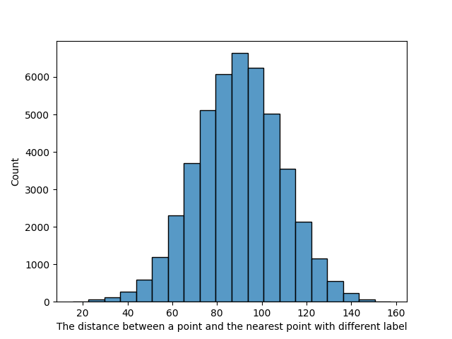
Figure 4: The histogram of the distance between a point and the nearest point with a different label. The data pool is merged across the pairwise condition, so the number of the data is $45000(=500*90)$.

4 Discussion

4.1 The interpretation of the theorems

Our theorems show the fundamental limitation of the AE in GP; the success probability of AE crafted by any method cannot exceed the value of MSP function $\phi$ in 1, and the vulnerability of a training dataset to the AE is determined by the closest pair of the data points whose labels are different.

The theorems can be applied to other inference models because GP includes some inference models. Especially, the theoretical bound can be computed for neural networks. Since neural networks with an infinite number of units in the hidden layer and Bayesian neural networks are regarded as GP [williams_computing_1996, gal_dropout_2016], our results are applicable to neural networks, resulting in giving the fundamental limitation of the AE in neural networks, like the previous research [shafahi_are_2019, blaas_adversarial_2020, fawzi_adversarial_2018]. Comparing the previous research, our result adds the viewpoint of the distance between the samples.

There are prior researches concerning the upper bound of adversarial robustness [blaas_adversarial_2020][cardelli_robustness_2019] [smith_adversarial_2023]. However, their upper bound is not easy to calculate against the real adversarial example (in terms of adversarial perturbation) and our theorems contribute to the adversarial robustness research in that we provide the upper bound easy to calculate and from the viewpoint of kernel function.

Though there are some studies that investigate human perception and adversarial perturbation, we excluded a notion of human perception from the definition of adversarial examples, and we simply proved the theorem for the samples with the $r$-perturbation from the training samples. We showed that the probability of misclassification of that sample varies by the kernel function and perturbation size and the closest points from both classes. This direction enables us to regard any samples in the input space as probabilistic adversarial examples and more rigorous investigation for them can be conducted.

4.2 The choice of kernel functions

Since the predictive mean can be written as the sum of the terms of the kernel functions whose inputs are each training point and test point (Representer Theorem in Gaussian Processes), changing the parameter of kernel functions changes the shape of the decision boundary.

The result of the experiments in Section 3 suggests that the upper bound of the probability changes according to the choice of the kernel functions. The increase of $\theta_{2}$ of the kernel function results in the smaller upper bound when the distance of two points is large. This suggests that changing the activation function of a neural network can improve the robustness of that neural network. The change according to the kernel parameter of the Gaussian kernel (Eq. 66) shown in the experiment in Section 3 can be interpreted as below:

• when $\theta_{1}$ changes, the value of the Gaussian kernel is multiplied by $\theta_{1}$. With regard to $\mu$ and $\sigma$ in 1, when $\theta_{1}$ becomes larger, $\mu$ will be unchanged and $\sigma$ will be larger. Considering that the MSP function (Eq. 5) is based on the CDF of Gaussian distribution and the CDF of Gaussian distribution is monotonically increasing with respect to $\sigma$ when $\mu>0$, the value of Eq. 5 is larger when $\theta_{1}$ is larger.

• When $\theta_{2}$ changes, the bandwidth of Gaussian distribution in the Gaussian kernel will be changed. Considering the form of the exponential function, if $\theta_{2}$ is larger, the absolute value of the derivative of the Gaussian kernel with respect to $\lVert x-x^{\prime}\rVert^{2}$ at the same point is smaller. This suggests that, if $\theta_{2}$ is larger, the decay of the value of the Gaussian kernel with respect to $\lVert x-x^{\prime}\rVert^{2}$ is slower, and the effect on the value of the Gaussian kernel by the distance of two points would be bigger in the interval focused in the experiment.

Since $\phi(r|\mathcal{D})$ is not easily differentiable with respect to $k(x_{1},x_{2})$, the discrete calculation is required to confirm whether the kernel function satisfied the constraint in Section 2.7 and to determine the kernel function for improving the robustness. However, it is reasonable that if $k(x_{1},x_{2})$ is small (that is, $x_{1}$ and $x_{2}$ is too far away), $x_{*}$, the point near $x_{1}$, cannot be classified as the same class as $x_{2}$.

The previous research showed that the activation functions in neural networks are equivalent to the kernel functions in GP[williams_computing_1996, lee_deep_2018]. Therefore, the theoretical result of this paper suggests the theoretical basis for the enhancement method that changes the activation function in neural networks. The previous studies suggest that changing the activation function in neural networks can enhance the robustness against AEs [goodfellow_explaining_2015, taghanaki_kernelized_2019, gowal_uncovering_2021]. Our result shows that the change of the kernel function induces the change of the theoretical upper bound of the successful AEs, and considering that the activation function in neural networks is the counterpart of the kernel function in GP, our result suggests that the robustness enhancement method by changing the activation functions in neural networks has the same basis as our result.

4.3 Open Problems

This paper has open problems below: these problems should be solved with further investigation.

• 1 is proven under the assumption that the effect of input points other than $x_{1},x_{2}$ to the predictive mean is less than $\epsilon$. When using the Gaussian kernel, this condition is reasonable because the value of the Gaussian kernel is decreased rapidly according to the distance of the input points, and it is confirmed in the experiment that even if $\epsilon$ is set to 0, over 98% of the points follow the theorem. The theorem under the condition of using another kernel function should be investigated further. In relation to this, Smith et al. [smith_adversarial_2023] suggest that other kernel functions can be written using Gaussian kernels.

• The experiment with neural networks should be conducted, in order to confirm that one can design a more robust activation function using 1.

4.4 Limitations

The research has the following limitations. The problem formulation of the research is binary classification, not multi-class classification. Finding the nearest point can be time-consuming if the number of input points increases. An efficient algorithm, such as a divide-and-conquer algorithm, should be investigated for the search for the nearest point. $\epsilon$ in 1 depends on the distribution of the training data, the evaluation of the size of $\epsilon$ is yet to be investigated (but as we wrote above, the fact that the theorem holds with high probability even if is 0 suggests that we can safely use the upper bound without 1 in practical use).

4.5 Conclusion

In this paper, through the proof of the theorems, we showed that in the GP classification, the probability of a successful attack of AE has an upper bound that is determined by the nearest point from the dataset, the perturbation size, and the kernel function. We proved it under the assumption that the value of the predictive mean of GP regression doesn’t differ greatly when only the nearest points from the two classes are used as the training data. The statement of theorems and the plausibility of assumptions are confirmed by the experiment using the images from ImageNet. The experiment showed that the parameter of kernel functions can change the theoretical upper bound of the probability of a successful attack of AE, suggesting that the kernel function’s choice affects the robustness against AE in the GP classification. Considering the equivalency of GPs and neural networks, the result will give an important insight into the robustness of neural networks against AEs.

The practical implication of the result is the following:

• The modification of kernel functions in GP affects the robustness of classifiers. Therefore, our findings suggest that one can adjust the model architecture for defensive purposes, fed back by the calculated robustness.

• The new upper bound of adversarial robustness is easy to calculate and hence easy to use in practice.

References

- [1] Ian J. Goodfellow, Jonathon Shlens, and Christian Szegedy. Explaining and Harnessing Adversarial Examples. International Conference on Learning Representations, March 2015.
- [2] Nicholas Carlini and David Wagner. Towards Evaluating the Robustness of Neural Networks. In 2017 IEEE Symposium on Security and Privacy (SP), pages 39–57, San Jose, CA, USA, May 2017. IEEE.
- [3] Reuben Feinman, Ryan R. Curtin, Saurabh Shintre, and Andrew B. Gardner. Detecting Adversarial Samples from Artifacts. arXiv:1703.00410 [cs, stat], November 2017.
- [4] Qi-Zhi Cai, Min Du, Chang Liu, and Dawn Song. Curriculum Adversarial Training. In International Joint Conference on Artificial Intelligence, May 2018.
- [5] Nicholas Carlini and David Wagner. Adversarial Examples Are Not Easily Detected: Bypassing Ten Detection Methods. Proceedings of the 10th ACM Workshop on Artificial Intelligence and Security, pages 3–14, November 2017.
- [6] Carl Edward Rasmussen and Christopher K. I. Williams. Gaussian processes for machine learning. Adaptive computation and machine learning. MIT Press, Cambridge, Mass, 2006. OCLC: ocm61285753.
- [7] Christopher K I Williams. Computing with Infinite Networks. Advances in Neural Information Processing Systems, page 7, 1996.
- [8] Ali Shafahi, W. Ronny Huang, Christoph Studer, Soheil Feizi, and Tom Goldstein. Are adversarial examples inevitable? 7th International Conference on Learning Representations, 2019.
- [9] Arno Blaas, Andrea Patane, Luca Laurenti, Luca Cardelli, Marta Kwiatkowska, and Stephen Roberts. Adversarial Robustness Guarantees for Classification with Gaussian Processes. Proceedings of the Twenty Third International Conference on Artificial Intelligence and Statistics,, 108:3372–3382, March 2020.
- [10] Luca Cardelli, Marta Kwiatkowska, Luca Laurenti, and Andrea Patane. Robustness Guarantees for Bayesian Inference with Gaussian Processes. The Thirty-Third AAAI Conference on Artificial Intelligence, 2019.
- [11] Yizhen Wang, Somesh Jha, and Kamalika Chaudhuri. Analyzing the Robustness of Nearest Neighbors to Adversarial Examples. Proceedings of the 35 th International Conference on Machine Learning, page 10, 2018.
- [12] Alhussein Fawzi, Hamza Fawzi, and Omar Fawzi. Adversarial vulnerability for any classifier. Proceedings of the 32nd International Conference on Neural Information Processing Systems., pages 1186–1195, November 2018.
- [13] Saeed Mahloujifar, Dimitrios I. Diochnos, and Mohammad Mahmoody. The Curse of Concentration in Robust Learning: Evasion and Poisoning Attacks from Concentration of Measure. Proceedings of the AAAI Conference on Artificial Intelligence, 33:4536–4543, July 2019.
- [14] Xiao Zhang, Jinghui Chen, Quanquan Gu, and David Evans. Understanding the intrinsic robustness of image distributions using conditional generative models. In Silvia Chiappa and Roberto Calandra, editors, Proceedings of the Twenty Third International Conference on Artificial Intelligence and Statistics, volume 108 of Proceedings of Machine Learning Research, pages 3883–3893. PMLR, 26–28 Aug 2020.
- [15] Beilun Wang, Ji Gao, and Yanjun Qi. A Theoretical Framework for Robustness of (Deep) Classifiers against Adversarial Examples. ICLR 2017 Workshop Section, September 2017.
- [16] Justin Gilmer, Luke Metz, Fartash Faghri, Samuel S. Schoenholz, Maithra Raghu, Martin Wattenberg, and Ian Goodfellow. The Relationship Between High-Dimensional Geometry and Adversarial Examples. arXiv:1801.02774 [cs], September 2018.
- [17] Arjun Nitin Bhagoji, Daniel Cullina, and Prateek Mittal. Lower Bounds on Adversarial Robustness from Optimal Transport. 33rd Conference on Neural Information Processing Systems, October 2019.
- [18] Jeremy M. Cohen, Elan Rosenfeld, and J. Zico Kolter. Certified Adversarial Robustness via Randomized Smoothing, June 2019. arXiv:1902.02918 [cs, stat].
- [19] Michael Thomas Smith, Kathrin Grosse, Michael Backes, and Mauricio A. Álvarez. Adversarial vulnerability bounds for Gaussian process classification. Machine Learning, 112(3):971–1009, March 2023.
- [20] Jaehoon Lee, Yasaman Bahri, Roman Novak, Samuel S. Schoenholz, Jeffrey Pennington, and Jascha Sohl-Dickstein. Deep Neural Networks as Gaussian Processes. International Conference on Learning Representations, March 2018.
- [21] Yarin Gal and Zoubin Ghahramani. Dropout as a Bayesian Approximation: Representing Model Uncertainty in Deep Learning. Proceedings of The 33rd International Conference on Machine Learning, 48:1050–1059, October 2016.
- [22] Saeid Asgari Taghanaki, Kumar Abhishek, Shekoofeh Azizi, and Ghassan Hamarneh. A Kernelized Manifold Mapping to Diminish the Effect of Adversarial Perturbations. In IEEE/CVF Conference on Computer Vision and Pattern Recognition. IEEE, 2019.
- [23] Sven Gowal, Chongli Qin, Jonathan Uesato, Timothy Mann, and Pushmeet Kohli. Uncovering the Limits of Adversarial Training against Norm-Bounded Adversarial Examples, March 2021. arXiv:2010.03593 [cs, stat].