High curvature means low-rank: On the sectional curvature of Grassmann and Stiefel manifolds and the underlying matrix trace inequalities

Abstract

Methods and algorithms that work with data on nonlinear manifolds are collectively summarised under the term ‘Riemannian computing’. In practice, curvature can be a key limiting factor for the performance of Riemannian computing methods. Yet, curvature can also be a powerful tool in the theoretical analysis of Riemannian algorithms. In this work, we investigate the sectional curvature of the Stiefel and Grassmann manifold from the quotient space view point. On the Grassmannian, tight curvature bounds are known since the late 1960ies. On the Stiefel manifold under the canonical metric, it was believed that the sectional curvature does not exceed 5/4. For both of these manifolds, the sectional curvature is given by the Frobenius norm of certain structured commutator brackets of skew-symmetric matrices. We provide refined inequalities for such terms and pay special attention to the maximizers of the curvature bounds. In this way, we prove that the global bound of 5/4 for Stiefel holds indeed. With this addition, a complete account of the curvature bounds in all admissible dimensions is obtained. We observe that ‘high curvature means low-rank’, more precisely, for the Stiefel and Grassmann manifolds, the global curvature maximum is attained at tangent plane sections that are spanned by rank-two matrices. Numerical examples are included for illustration purposes.

15B10, 15B57, 15B30, 65F99, 22E70, 53C30, 53C80,

1 Introduction

Methods and algorithms that work with data on nonlinear manifolds are collectively summarised under the term Riemannian computing. Riemannian computing methods have established themselves as important tools in a large variety of applications, including computer vision, machine learning, and optimization, see [1, 2, 5, 8, 10, 18, 24, 25] and the anthologies [19, 26]. They also gain increasing attention in statistics and data science [22] and in numerical methods for differential equations [6, 7, 13, 16, 31].
A standard technique in designing Riemannian computing methods is to translate Euclidean algorithms to manifolds. The discrepancy between a linear space and a non-linear manifold is quantified by the concept of curvature. Therefore, curvature can also be seen as a decisive factor that separates Riemannian algorithms from their Euclidean counterparts. On the other hand, curvature can be a powerful tool in the theoretical analysis of Riemannian methods; curvature estimates allow to compare Euclidean distances and Riemannian distances for embedded submanifolds [4], and they give bounds on the injectivity radius of the manifold in quesion, see [23, Section 6]. This has been exploited to obtain explicit bounds on the Stiefel manifold’s injectivity radius in [25] and very recently in [3].

In this work, we investigate the sectional curvature on the Stiefel and Grassmann manifolds from the quotient space view point. Both of these manifolds have been subject to extensive investigations before. On the Grassmannian, tight curvature bounds are known since the seminal papers of Wong [28, 29]. The sectional curvature on the Stiefel manifold under a parametric family of Riemannian metrics introduced in [15] was extensively studied in [20]. On the Stiefel manifold under the canonical metric, it was believed that the sectional curvature does not exceed $5/4$, [25, p. 94,95], [20, Section 6, Table 2]. Nguyen [20] shows that the bound is tight for the Stiefel manifold of orthogonal $p$-frames if $p=2$, but a valid proof for general $p\geq 2$ was missing.

For the orthogonal group and, in turn, for the Stiefel and Grassmann manifolds as its quotient spaces, the sectional curvature is given by the Frobenius norm of certain structured commutator brackets of skew-symmetric matrices. Sharp estimates are provided by the matrix inequality of [30] and the special bounds for skew-symmetric matrices of [11, Lemma 2.5]. We provide refined inequalities for such terms and pay special attention to the maximizers of the curvature bounds. In this way, we prove that the global bound of 5/4 for Stiefel holds indeed.

In doing so, we observe that ‘high curvature means low-rank’. To be precise, we prove that for the orthogonal group and the Stiefel and Grassmann manifolds, the global curvature maximum is attained at tangent plane sections that are spanned by the same low-rank tangent matrices. From the perspective of the orthogonal group, these are rank-four matrices, while they are rank-two matrices from the Stiefel or Grassmann view point. Numerical experiments confirm that the curvature drops with increasing rank.

Organisation of the paper

Section 2 provides the required curvature formulas for matrix Lie groups and their quotient spaces. (For the reader’s convenience, some essentials of Lie group theory is gathered in Section C.1.) Readers not interested in the matrix manifold applications but only in the matrix norm inequalities may directly skip to Section 3. In this section, we also give a full account of the sharp Stiefel curvature bounds in all possible dimensions. Numerical experiments are discussed in Section 4. Section 5 concludes the paper.

Notational specifics

For $n\in\mathbb{N}$, the $(n\times n)$-identity matrix is denoted by $I_{n}\in\mathbb{R}^{n\times n}$, or simply $I$, if the dimension is clear. The $(n\times n)$ special orthogonal group, i.e., the set of all square orthogonal matrices with determinant $1$ is denoted by

$$SO(n)=\{Q\in\mathbb{R}^{n\times n}|Q^{T}Q=QQ^{T}=I_{n}\}.$$

The orthogonal group $O(n)$ is $SO(n)$ joint with their ‘$\det=-1$’-siblings. The sets of symmetric and skew-symmetric $(n\times n)$-matrices are $\operatorname{sym}(n)=\{A\in\mathbb{R}^{n\times n}|A^{T}=A\}$ and $\operatorname{skew}(n)=\{A\in\mathbb{R}^{n\times n}|A^{T}=-A\}$, respectively. Overloading this notation, $\operatorname{sym}(A)=\frac{1}{2}(A+A^{T}),\operatorname{skew}(A)=\frac{1}{2}(A-A^{T})$ denote the symmetric and skew-symmetric parts of a matrix $A$. The Stiefel manifold is

$$St(n,p)=\{U\in\mathbb{R}^{n\times p}\mid U^{T}U=I_{p}\}.$$

The Grassmann manifold is

$$Gr(n,p)=\{[U]\mid U\in St(n,p)\},\text{where }[U]=\{UR\mid R\in SO(p)\}.$$

A word of caution: The standard Euclidean inner product on $\mathbb{R}^{n\times p}$ is

$$\langle X,Y\rangle_{F}=\operatorname{tr}(X^{T}Y).$$

The subscript is to emphazise the correspondence with the Frobenius norm $\|X\|_{F}=\sqrt{\langle X,X\rangle_{F}}$. To comply with standard conventions in the matrix manifolds and Riemannian computing literature, the Riemannian metric on $SO(n)$ will not be the Euclidean one, but the Euclidean one with a multiplicative factor of $\frac{1}{2}$, i.e.,

(1) $$\langle X,Y\rangle_{Q}=\frac{1}{2}\operatorname{tr}(X^{T}Y)=\frac{1}{2}\langle X,Y\rangle_{F},\quad X,Y\in T_{Q}SO(n).$$

This factor is inherited by the Riemannian metrics of the Grassmann and the Stiefel manifold, when considered as quotients of $SO(n)$. It also makes the curvature results in this work compatible with those stated, e.g., in the seminal papers [28, 29]. To distinguish the Riemannian and the Euclidean metric, for the former, the location is always given as a subscript $\langle\cdot,\cdot\rangle_{Q}$.

Let $\mathcal{M}$ be a quotient of $SO(n)$ under a Lie group action. (We will only consider $\mathcal{M}=St(n,p)$ or $\mathcal{M}=Gr(n,p)$.) For a tangent vector $X\in T_{I}SO(n)=\mathfrak{so}(n)=\operatorname{skew}(n)$, $X_{\mathfrak{m}}$ denotes the projection onto the horizontal space associated with $\mathcal{M}$. When a distinction is necessary, we will also write $X_{\mathfrak{m}^{\mathcal{M}}}$ to emphasize, which quotient manifold is considered. Likewise, $X_{\mathfrak{h}}$ and $X_{\mathfrak{h}^{\mathcal{M}}}$ denote the projection onto the vertical space associated with $\mathcal{M}$.

2 Curvature of Lie groups and quotients of Lie groups

This section recaps the basic curvature formulas for Lie groups and quotients of Lie groups. This is classic textbook material. Our main references are [9], [14] and [21], to which we refer for the details. Readers not familiar with Lie groups or quotients of Lie groups may want to read Appendix C first.

2.1 Lie group curvature formulae

Let $\mathcal{G}$ be a Lie group with Lie algebra $\mathfrak{g}=T_{I}\mathcal{G}$ (the tangent space at $I$) and a bi-invariant metric. Let $X,Y\in\mathfrak{g}$ be linearly independent tangent vectors. The sectional curvature associated with the two-dimensional subplane spanned by $\{X,Y\}\subset\mathfrak{g}$ is

$$K(X,Y)=\frac{1}{4}\frac{\|[X,Y]\|_{I}^{2}}{\|X\|_{I}^{2}\|Y\|_{I}^{2}-\langle X,Y\rangle_{I}},$$

where $[X,Y]=XY-YX$. It depends only on the subplane, in this context often referred to as ‘the section’, not on the spanning vectors $X,Y$. For convenience, we will only consider $X,Y\in\mathfrak{g}$ forming an orthonormal basis (ONB), i.e., $\|X\|_{I}=1=\|Y\|_{I}$, $\langle X,Y\rangle_{I}=0$, so that the sectional curvature is computed as

(2) $$K(X,Y)=\frac{1}{4}\|[X,Y]\|_{I}^{2},$$

see [9, Prop. 21.19, p. 636].

Remark.

For $\mathcal{G}=SO(n)$, we use the metric of (1). Hence, when translated to the Frobenius norm, one has

$$K^{SO}(X,Y)=\frac{1}{2}\|[X,Y]\|_{F}^{2},\quad\text{for }\|X\|_{F}=1=\|Y\|_{F},\quad\langle X,Y\rangle_{F}=0.$$

In order to obtain curvature expressions for Lie group quotients, we need to introduce a few more terms. The adjoint map ${\bf Ad}:\mathcal{G}\to GL(\mathcal{G})$ assigns to each group element $A\in\mathcal{G}$ the linear map ${\bf Ad}_{A}:B\mapsto ABA^{-1}$. Note that ${\bf Ad}_{A}(I)=I$. The differential of ${\bf Ad}_{A}$ at $I$ is the map $\operatorname{Ad}_{A}:=d({\bf Ad}_{A})_{I}:T_{I}\mathcal{G}=\mathfrak{g}\to\mathfrak{g}=T_{{\bf Ad}_{A}(I)}\mathcal{G}$. For a matrix Lie group, $\operatorname{Ad}_{A}(X)=AXA^{-1}$.

The homogeneous $\mathcal{G}$-space $\mathcal{G}/\mathcal{H}$ is reductive, if the Lie algebra $\mathfrak{g}$ (the tangent space at the identity) can be split into

$$\mathfrak{g}=\mathfrak{h}\oplus\mathfrak{m},$$

where $\mathfrak{h}$ is the Lie algebra of $\mathcal{H}$ (the tangent space at the identity) and $\mathfrak{m}\subset\mathfrak{g}$ is a complementary subspace such that $\operatorname{Ad}_{Q}(\mathfrak{m})\subseteq\mathfrak{m}$ for all $Q\in H$. Note that while the setting above is more general, in the cases that we eventually consider in this work, $\mathfrak{m}$ will always be the orthogonal complement of $\mathfrak{h}$ with respect to a suitable metric. For a tangent vector $X\in\mathfrak{g}$, the projections onto $\mathfrak{h}$ and $\mathfrak{m}$ are denoted by $X_{\mathfrak{h}}$ and $X_{\mathfrak{m}}$, respectively.

The quotient space $\mathcal{G}/\mathcal{H}$ is called naturally reductive, if

1. it is reductive with some decomposition $\mathfrak{g}=\mathfrak{h}\oplus\mathfrak{m}$,

2. it has a $\mathcal{G}$-invariant metric,

3. $\langle[X,Z]_{\mathfrak{m}},Y\rangle_{I}=\langle X,[Z,Y]_{\mathfrak{m}}\rangle_{I}$ for all $X,Y,Z\in\mathfrak{m}$.

Item (ii) means that the maps $\tau_{G}:\mathcal{G}/\mathcal{H}\to\mathcal{G}/\mathcal{H},[A]\mapsto G\cdot[A]$ associated with the action $\mathcal{G}\times\mathcal{G}/\mathcal{H}\to\mathcal{H},(G,[A])\mapsto G\cdot[A]$ are isometries. The precise condition is

$$\langle d(\tau_{G})_{[A]}(X),d(\tau_{G})_{[A]}(Y)\rangle_{\tau_{G}([A])}=\langle X,Y\rangle_{[A]}\quad\forall X,Y\in T_{[A]}\mathcal{G}/\mathcal{H},[A]\in\mathcal{G}/\mathcal{H},$$

[9, Def. 23.5]. On the level of matrix representatives (and after identifying $T_{[A]}\mathcal{G}/\mathcal{H}$ with the horizontal space $H_{A}$), this boils down to the condition

$$\langle G\bar{X},G\bar{Y}\rangle_{GA}=\langle\bar{X},\bar{Y}\rangle_{A}\text{ for all }\bar{X},\bar{Y}\in H_{A},A\in\mathcal{G},$$

where $\bar{X},\bar{Y}\in H_{A}$ are horizontal lifts of $X,Y\in T_{[A]}\mathcal{G}/\mathcal{H}$.

Theorem ([9], Prop. 23.29).

Let $\mathcal{G}$ be a connected Lie group such that the Lie algebra $\mathfrak{g}$ admits an $\operatorname{Ad}(\mathcal{G})$-invariant inner product $\langle\cdot,\cdot\rangle_{I}$. Let $\mathcal{G}/\mathcal{H}$ be a homogeneous space as above and let $\mathfrak{m}=\mathfrak{h}^{\bot}$ with respect to $\langle\cdot,\cdot\rangle_{I}$. Then

1. The space $\mathcal{G}/\mathcal{H}$ is reductive with respect to the decomposition $\mathfrak{g}=\mathfrak{h}\oplus\mathfrak{m}$.

2. Under the $\mathcal{G}$-invariant metric induced by the inner product, the homogeneous space $\mathcal{G}/\mathcal{H}$ is naturally reductive.

3. For an ONB spanned by $X,Y\in T_{[I]}\mathcal{G}/\mathcal{H}\cong\mathfrak{m}$, $X\bot Y$, $\|X\|_{I}=\|Y\|_{I}=1$, the sectional curvature associated with the tangent plane spanned by $X,Y$ is

   (3) $$K(X,Y)=\frac{1}{4}\|[X,Y]_{\mathfrak{m}}\|^{2}_{I}+\|[X,Y]_{\mathfrak{h}}\|_{I}^{2}.$$

Transport to arbitrary locations

Since the tangent space at an arbitrary location $A\in\mathcal{G}$ is given by the translates of the tangent space at the identity (see (29)), a tangent vector $\tilde{X}\in T_{A}\mathcal{G}$ at an arbitrary location $A\in\mathcal{G}$ is of the form $\tilde{X}=AX$ with $X\in\mathfrak{g}$. For an ONB $\{\tilde{X}=AX,\tilde{Y}=AY\}$ that spans a tangent plane in $T_{A}\mathcal{G}$, the sectional curvature is

$$K^{\mathcal{G}}(\tilde{X},\tilde{Y})=\frac{1}{4}\|[X,Y]\|_{I}^{2}.$$

For quotient spaces, because of the natural reductive homogeneous space structure, the horizontal spaces $H_{A}$ at arbitrary locations $A\in\mathcal{G}$ are translates of the horizontal space $\mathfrak{m}\cong T_{[I]}\mathcal{G}/\mathcal{H}$. Therefore, the tangent space of the quotient $\mathcal{G}/\mathcal{H}$ is identified with

$$T_{[A]}\mathcal{G}/\mathcal{H}\cong H_{A}=A\mathfrak{m}.$$

Let $\tilde{X},\tilde{Y}\in T_{[A]}\mathcal{G}/\mathcal{H}$ be an ONB of a tangent plane in the quotient space. Let $\bar{X},\bar{Y}\in H_{A}\subset T_{A}\mathcal{G}$ be horizontal lifts of $\tilde{X},\tilde{Y}\in T_{[A]}\mathcal{G}/\mathcal{H}\cong A\mathfrak{m}$ with $\bar{X}=AX,\bar{Y}=AY$, $X,Y\in\mathfrak{m}$. Then the sectional curvature at $[A]\in T_{[A]}\mathcal{G}/\mathcal{H}$ with respect to the tangent plane is given by

(4) $$K^{\mathcal{G}/\mathcal{H}}(\tilde{X},\tilde{Y})=\frac{1}{4}\|[X,Y]_{\mathfrak{m}}\|^{2}_{I}+\|[X,Y]_{\mathfrak{h}}\|^{2}_{I}.$$

For details, see [9, §19–23].

2.2 Curvature formulae on Grassmann and canonical Stiefel

In this section we recap the expressions for the sectional curvature on the Grassmann and the Stiefel manifold. Both the Stiefel manifold $St(n,p)$ and the Grassmann manifold $Gr(n,p)$ are considered as quotients of $SO(n)$. The Riemannian metric on the total space $SO(n)$ is

(5) $$\langle X,Y\rangle_{Q}=\frac{1}{2}\operatorname{tr}(X^{T}Y),\quad X,Y\in T_{Q}SO(n)=Q\operatorname{skew}(n).$$

All conditions of Theorem Theorem are fulfilled for $\mathcal{G}=SO(n)$ with this metric and its quotient spaces $St(n,p)$ and $Gr(n,p)$.

Grassmann sectional curvature

The Grassmann manifold of linear subspaces can be realized as the quotient space $Gr(n,p)=SO(n)/(SO(p)\times SO(n-p))$. The canonical projection and the left cosets are

$$\Pi^{Gr} : SO(n)\to Gr(n,p)$$

$$[Q]=:\Pi^{Gr}(Q) = \{Q\begin{pmatrix}S&0\\ 0&R\end{pmatrix}\mid\begin{pmatrix}S&0\\ 0&R\end{pmatrix}\in SO(p)\times SO(n-p)\}.$$

By splitting $Q=\begin{pmatrix}[c|c]U&U_{\bot}\end{pmatrix}$ with $U\in\mathbb{R}^{n\times p},U_{\bot}\in\mathbb{R}^{n\times(n-p)}$, $[Q]\in Gr(n,p)$ is uniquely represented by $\operatorname{ran}(U)\subset\mathbb{R}^{n}$.
When lifting $[Q]\in Gr(n,p)$ to $Q\in SO(n)$ (in practice, this is nothing but fixing a representative $Q$ for the equivalence class $[Q]$), the vertical space is represented by

$$V_{Q}^{Gr}=\bigl{\{}\bar{X}=Q\begin{pmatrix}A&0\\ 0&C\end{pmatrix}\mid A\in\operatorname{skew}(p),C\in\operatorname{skew}(n-p)\bigr{\}}=Q\mathfrak{h}^{Gr}.$$

The associated horizontal space is

$$T_{[Q]}Gr(n,p)\cong H_{Q}^{Gr}=\bigl{\{}\bar{X}=Q\begin{pmatrix}0&-B^{T}\\ B&0\end{pmatrix}\mid B\in\mathbb{R}^{(n-p)\times p}\bigr{\}}=Q\mathfrak{m}^{Gr}.$$

For Grassmann tangent vectors (already represented in matrix form by their lifts) $X=\begin{pmatrix}0&-B^{T}_{1}\\ B_{1}&0\end{pmatrix},Y=\begin{pmatrix}0&-B^{T}_{2}\\ B_{2}&0\end{pmatrix}\in\mathfrak{m}^{Gr}\cong T_{[I]}Gr(n,m)$, it holds that $X,Y$ are orthonormal w.r.t. (5) if and only if $B_{1},B_{2}\in\mathbb{R}^{(n-p)\times p}$ are orthonormal w.r.t. the standard Euclidean inner product $\langle\cdot,\cdot\rangle_{F}$. For such orthonormal $X,Y$, a straightforward evaluation of (3) yields

(6) $$K^{Gr}(X,Y) = \frac{1}{4}\|[X,Y]_{\mathfrak{m}^{Gr}}\|^{2}_{[I]}+\|[X,Y]_{\mathfrak{h}^{Gr}}\|^{2}_{[I]}$$

$$= \frac{1}{2}\|B_{1}^{T}B_{2}-B_{2}^{T}B_{1}\|_{F}^{2}+\frac{1}{2}\|B_{1}B_{2}^{T}-B_{2}B_{1}^{T}\|_{F}^{2}$$

(7) $$= \operatorname{tr}(B_{1}^{T}B_{2}B_{2}^{T}B_{1})+\operatorname{tr}(B_{1}B_{2}^{T}B_{2}B_{1}^{T})-2\operatorname{tr}(B_{1}^{T}B_{2}B_{1}^{T}B_{2}).$$

Stiefel sectional curvature

The Stiefel manifold of orthonormal $p$-frames can be realized as the quotient space $St(n,p)=SO(n)/SO(n-p)$. The canonical projection and the left cosets are

$$\Pi^{St} : SO(n)\to St(n,p)$$

$$[Q]=:\Pi^{St}(Q) = \{Q\begin{pmatrix}I&0\\ 0&R\end{pmatrix}\mid R\in SO(n-p)\}.$$

By splitting $Q=\begin{pmatrix}[c|c]U&U_{\bot}\end{pmatrix}$, $[Q]\in St(n,p)$ is uniquely determined by $U\in\mathbb{R}^{n\times p}$.
When lifting $[Q]\in St(n,p)$ to $Q\in SO(n)$, the vertical space is represented by

$$V_{Q}^{St}=\bigl{\{}\bar{X}\in\mathbb{R}^{n\times n}\mid\bar{X}=Q\begin{pmatrix}0&0\\ 0&C\end{pmatrix},\\ C\in\operatorname{skew}(n-p)\bigr{\}}=Q\mathfrak{h}^{St}.$$

The associated horizontal space is

$$T_{[Q]}St(n,p)\cong H_{Q}^{St}=\bigl{\{}\bar{X}=Q\begin{pmatrix}A&-B^{T}\\ B&0\end{pmatrix}\mid\\ A\in\operatorname{skew}(p),B\in\mathbb{R}^{(n-p)\times p}\bigr{\}}=Q\mathfrak{m}^{St}.$$

For tangent vectors $X=\begin{pmatrix}A_{1}&-B^{T}_{1}\\ B_{1}&0\end{pmatrix},Y=\begin{pmatrix}A_{2}&-B^{T}_{2}\\ B_{2}&0\end{pmatrix}\in\mathfrak{m}^{St}\cong T_{[I]}St(n,p)$ that are orthonormal w.r.t. (5), a straightforward evaluation of (3) yields

(8) $$K^{St}(X,Y) = \frac{1}{4}\|[X,Y]_{{\mathfrak{m}}^{St}}\|^{2}_{[I]}+\|[X,Y]_{\mathfrak{h}^{St}}\|^{2}_{[I]}$$

$$= \frac{1}{2}\|B_{2}B_{1}^{T}-B_{1}B_{2}^{T}\|_{F}^{2}+\frac{1}{4}\|B_{1}A_{2}-B_{2}A_{1}\|_{F}^{2}$$

$$+\frac{1}{8}\|[A_{1},A_{2}]-(B_{1}^{T}B_{2}-B_{2}^{T}B_{1})\|_{F}^{2}.$$

This is in line with the result of [20, Prop 4.2, eq. (34)].

3 Matrix norm inequalities and curvature estimates

In this section, we investigate the extremal behavior of the sectional curvature on the Grassmann and the Stiefel manifold. It is known since [29], that the sectional curvature on the Grassmann manifold ranges in the interval $[0,2]$ with both the lower and the upper bound attained. The upper bound can be established by using the matrix inequality

(9) $$\|B_{1}B_{2}^{T}-B_{2}B_{1}^{T}\|_{F}^{2}\leq 2\|B_{1}\|_{F}^{2}\|B_{2}\|^{2}_{F}$$

of Wu and Chen, [30].

Applying (9) to the terms (6) and keeping $\|B_{1}\|_{F}=1=\|B_{2}\|_{F}$ in mind immediately gives $0\leq K^{Gr}(X,Y)\leq 2$. A key idea in [30] is to exploit the skew-symmetry of the real Schur form of $B_{1}B_{2}^{T}-B_{2}B_{1}^{T}$. They also show by algebraic means that the inequality is sharp if and only if

$$B_{1}=\begin{pmatrix}[c|c]\begin{matrix}0&1\\ \lambda&\mu\end{matrix}&\mathbf{0}\\ \hline\cr\mathbf{0}&\mathbf{0}\\ \end{pmatrix},\quad B_{2}=\begin{pmatrix}[c|c]\begin{matrix}\lambda&\mu\\ 0&-1\end{matrix}&\mathbf{0}\\ \hline\cr\mathbf{0}&\mathbf{0}\\ \end{pmatrix},$$

up to an orthogonal transformation and scaling. Hence, under the normalization constraint $\|B_{1}\|_{F}=1=\|B_{2}\|_{F}$, both terms in (6) attain their upper bound of $2$ simultaneously for the rank-2 matrices

$$B_{1}=\frac{1}{\sqrt{2}}\begin{pmatrix}[c|c]\begin{matrix}0&1\\ 1&0\end{matrix}&\mathbf{0}\\ \hline\cr\mathbf{0}&\mathbf{0}\\ \end{pmatrix},\quad B_{2}=\frac{1}{\sqrt{2}}\begin{pmatrix}[c|c]\begin{matrix}1&0\\ 0&-1\end{matrix}&\mathbf{0}\\ \hline\cr\mathbf{0}&\mathbf{0}\\ \end{pmatrix}.$$

Observe that $\langle B_{1},B_{2}\rangle_{F}=0$. Hence, this matrix pair forms an ONB and so do the associated Grassmann tangent vectors.

To gain more insight on how the various trace terms contribute to the overall curvature value, we will re-establish this result via an optimization approach. To this end, we will consider the three trace terms

$$\operatorname{tr}(B_{1}^{T}B_{2}B_{2}^{T}B_{1}),\mbox{ }\operatorname{tr}(B_{1}B_{2}^{T}B_{2}B_{1}^{T}),\mbox{ and }-2\operatorname{tr}(B_{1}^{T}B_{2}B_{1}^{T}B_{2})\quad B_{1},B_{2}\in\mathbb{R}^{(n-p)\times p},$$

in the curvature expression (7) separately. Eventually, this will leads to an alternative proof and a refinement of the matrix inequality of Wu and Chen, [30]. We start with a preparatory lemma that improves on the classical submultiplicativity property $\|AB\|_{F}\leq\|A\|_{F}\|B\|_{F}$.

Lemma.

Let $A\in\mathbb{R}^{n\times m}$, $B\in\mathbb{R}^{m\times p}$. Then

(10) $$\|AB\|_{F}\leq\min\{\|A\|_{2}\|B\|_{F},\|A\|_{F}\|B\|_{2}\}.$$

If either $A$ or $B$ is skew-symmetric, then

(11) $$\|AB\|_{F}\leq\frac{1}{\sqrt{2}}\|A\|_{F}\|B\|_{F}.$$

Proof.

On (10): First, consider $D\in\mathbb{R}^{m\times m}$ diagonal. Write $B=(b_{1},\ldots,b_{p})$ column-wise. It holds

$$\|DB\|^{2}_{F} = \operatorname{tr}(B^{T}D^{2}B)=\sum_{j=1}^{p}b_{j}^{T}D^{2}b_{j}=\sum_{j=1}^{p}\|b_{j}\|_{2}^{2}\frac{b_{j}^{T}D^{2}b_{j}}{b_{j}^{T}b_{j}}$$

$$\leq \max_{j}\{d_{j}^{2}\}\sum_{j=1}^{p}\|b_{j}\|_{2}^{2}=\|D\|_{2}^{2}\|B\|_{F}^{2}.$$

The general case can be reduced to this case. Let $U\Sigma V^{T}=A$ be the full SVD of $A$.

$$\|AB\|_{F}^{2} = \|U\Sigma V^{T}B\|_{F}^{2}=\operatorname{tr}(B^{T}V\Sigma^{T}\Sigma V^{T}B)$$

$$= \|\sqrt{\Sigma^{T}\Sigma}V^{T}B\|_{F}^{2}\stackrel{{\scriptstyle D=\sqrt{\Sigma^{T}\Sigma}}}{{=}}\sigma_{1}^{2}\|V^{T}B\|_{F}^{2}=\|A\|_{2}^{2}\|B\|_{F}^{2}.$$

When working with the SVD of $B$, the same argument may be applied to $\|B^{T}A^{T}\|^{2}_{F}$ and yields $\|B^{T}A^{T}\|^{2}_{F}\leq\|B^{T}\|_{2}^{2}\|A^{T}\|_{F}^{2}=\|B\|_{2}^{2}\|A\|_{F}^{2}$.
The second inequality (11) comes as a corollary. W.l.o.g. assume that $A\in\operatorname{skew}(m)$. Then, all eigenvalues of $A$ are either zero or form purely imaginary, complex conjugate pairs. The singular values of $A$ are the absolute values of the eigenvalues of $A$. Therefore, the singular values also come in pairs. Let $\sigma_{1}=\sigma_{2}\geq\dots\geq\sigma_{r-1}=\sigma_{r}>0$ be the non-zero singular values of $A$. We obtain

$$\|A\|_{2}^{2}=\sigma_{1}^{2}=\frac{1}{2}\left(\sigma_{1}^{2}+\sigma_{2}^{2}\right)\leq\frac{1}{2}\left(\sigma_{1}^{2}+\sigma_{2}^{2}+\dots+\sigma_{r}^{2}\right)=\frac{1}{2}\|A\|_{F}^{2}.$$

Hence, (10) yields $\|AB\|_{F}\leq\|A\|_{2}\|B\|_{F}\leq\frac{1}{\sqrt{2}}\|A\|_{F}\|B\|_{F}$.

Alternatively, (10) can also be established as a consequence of [27, Lemma 1].

The following lemma is obvious.

Lemma.

Let $m\geq p$ and consider $B_{2}\in\mathbb{R}^{m\times p}$ as fixed. Let $U\Sigma V^{T}=B_{2}$ be the (full) SVD of $B_{2}$ with $\Sigma=\begin{pmatrix}\Sigma_{p}\\ \mathbf{0}\end{pmatrix}\in\mathbb{R}^{m\times p}$ and $\Sigma_{p}=\mbox{diag}(\sigma_{1},\ldots,\sigma_{p})$.

1. The global optimum of

   $$\max_{B_{1}\in\mathbb{R}^{m\times p}}\operatorname{tr}(B^{T}_{1}B_{2}B_{2}^{T}B_{1})\quad\mbox{s.t. }\|B_{1}\|_{F}=1$$

   is $\sigma_{1}^{2}$ and is attained for any normalized $B_{1}$ such that $\tilde{B}_{1}:=U^{T}B_{1}V$ only features scaled copies of the first unit vector $e_{1}=(\pm 1,0,\ldots,0)^{T}\in\mathbb{R}^{m}$ as columns.

2. The global optimum of

   $$\max_{B_{1}\in\mathbb{R}^{m\times p}}\operatorname{tr}(B_{1}B_{2}^{T}B_{2}B^{T}_{1})\quad\mbox{s.t. }\|B_{1}\|_{F}=1$$

   is $\sigma_{1}^{2}$ and is attained for any normalized $B_{1}$ such that $\tilde{B}_{1}:=U^{T}B_{1}V$ only features scaled copies of the first unit vector $e_{1}=(\pm 1,0,\ldots,0)^{T}\in\mathbb{R}^{p}$ as rows.

The next lemma concerns the third trace term in (7).

Lemma.

Let $m\geq p$ and let $B_{2}=U\Sigma V^{T}\in\mathbb{R}^{m\times p}$ (not necessarily normalized). Then

$$\max_{B_{1}\in\mathbb{R}^{m\times p},\|B_{1}\|_{F}=1}\operatorname{tr}(B^{T}_{1}B_{2}B^{T}_{1}B_{2}) = \sigma_{1}^{2},$$

$$\min_{B_{1}\in\mathbb{R}^{m\times p},\|B_{1}\|_{F}=1}\operatorname{tr}(B^{T}_{1}B_{2}B^{T}_{1}B_{2}) = -\sigma_{1}\sigma_{2}.$$

The global maximum and minimum are attained for $B_{1}^{+}=U\tilde{B}_{1}^{+}V^{T}$ and $B_{1}^{-}=U\tilde{B}_{1}^{-}V^{T}$, where

(12) $$\tilde{B}_{1}^{+}=\pm\begin{pmatrix}[c|c]\begin{matrix}1&0\\ 0&0\end{matrix}&\mathbf{0}\\ \hline\cr\mathbf{0}&\mathbf{0}\\ \end{pmatrix},\mbox{ and }\tilde{B}_{1}^{-}=\pm\frac{1}{\sqrt{2}}\begin{pmatrix}[c|c]\begin{matrix}0&1\\ -1&0\end{matrix}&\mathbf{0}\\ \hline\cr\mathbf{0}&\mathbf{0}\\ \end{pmatrix},\mbox{ respectively.}$$

For $B_{1},B_{2}$ both of unit Frobenius norm,

$$-\frac{1}{2}\leq\operatorname{tr}(B_{1}^{T}B_{2}B^{T}_{1}B_{2})\leq 1.$$

In this case, the global extrema are attained for $B_{1}^{+},B_{1}^{-}$ as above and $B_{2}^{+}$ of rank one ($\sigma_{1}=1$) and $B_{2}^{-}$ of rank 2 ($\sigma_{1}=\sigma_{2}=\frac{1}{\sqrt{2}}$).

Remark.

The extrema may not be isolated nor are they necessarily unique (up to the trace-preserving transformation). If $m=p$, $B_{2}=\sigma I$, then any normalized symmetric $B_{1}$ yields the maximum $\operatorname{tr}(B^{T}_{1}B_{2}B^{T}_{1}B_{2})=\sigma^{2}\|B_{1}\|^{2}_{F}=\sigma^{2}_{1}$. Likewise, any normalized skew-symmetric $B_{1}$ yields the minimum $\operatorname{tr}(B^{T}_{1}B_{2}B^{T}_{1}B_{2})=-\sigma^{2}\|B_{1}\|^{2}_{F}=-\sigma^{2}=(-\sigma_{1}\sigma_{2})$. However, for both $B_{1}$ and $B_{2}$ of unit Frobenius norm, the global extrema are attained only for the matrices in (12) (up to the trace preserving transformation).

Proof (Lemma Lemma).

Let $B_{2}=U\Sigma V^{T}\in\mathbb{R}^{m\times p}$ be the full SVD of $B_{2}$. Under the norm-preserving bijection $B\mapsto U^{T}BV=:\tilde{B}$, the trace optimization problem $\min_{B\in\mathbb{R}^{m\times p},\|B\|_{F}=1}\pm\operatorname{tr}(B^{T}B_{2}B^{T}B_{2})$ becomes $\min_{\tilde{B}\in\mathbb{R}^{m\times p},\|\tilde{B}\|_{F}=1}\pm\operatorname{tr}(\tilde{B}^{T}\Sigma\tilde{B}^{T}\Sigma)$.

Write $\Sigma=\begin{pmatrix}\Sigma_{p}\\ \mathbf{0}\end{pmatrix}$ and $\tilde{B}=\begin{pmatrix}\tilde{B}_{p}\\ \tilde{B}_{m-p}\end{pmatrix}$, with empty lower blocks if $m=p$. As a preliminary, observe that $\operatorname{tr}(\tilde{B}_{p}^{T}\tilde{B}_{p}^{T})=\langle\tilde{B}_{p},\tilde{B}^{T}_{p}\rangle_{F}=\sum_{j=1}^{p}\sum_{k=1}^{p}b_{jk}b_{kj}$. It holds

(13) $$\operatorname{tr}(\tilde{B}^{T}\Sigma\tilde{B}^{T}\Sigma) =\sum_{j=1}^{p}\sum_{k=1}^{p}\sigma_{j}\sigma_{k}b_{jk}b_{kj}$$

$$=\sigma_{1}^{2}b_{11}^{2}+\sum_{k=2}^{p}\sigma_{1}\sigma_{k}b_{1k}b_{k1}+\sum_{j=2}^{p}\left(\sigma_{j}\sigma_{1}b_{j1}b_{1j}+\sum_{k=2}^{p}\sigma_{j}\sigma_{k}b_{jk}b_{kj}\right)$$

$$\leq\sigma_{1}^{2}\langle\tilde{B}_{p},\tilde{B}_{p}^{T}\rangle_{F}\leq\sigma_{1}^{2}\|\tilde{B}\|_{F}^{2}=\sigma_{1}^{2}.$$

The maximum is attained, if all weight in $\tilde{B}$ is put on the upper diagonal entry, i.e., for $\tilde{B}^{+}$ as in the statement of the lemma. If $\sigma_{1}>\sigma_{2}$, then the maximum is isolated.

Now on the minimum. Reconsider (13) and extract the ‘diagonal terms’,

$$\operatorname{tr}(\tilde{B}^{T}\Sigma\tilde{B}^{T}\Sigma)=\sum_{j=1}^{p}\sum_{k=1,k\neq j}^{p}\sigma_{j}\sigma_{k}b_{jk}b_{kj}+\sum_{j=1}^{p}{\sigma_{j}^{2}b_{jj}^{2}}.$$

One sees that the diagonal terms in $\tilde{B}_{p}$ only make nonnegative contributions to the trace total. All remaining terms become non-positive, if $b_{jk}$ and $b_{kj}$ are of opposite sign for all $k\neq j$. In this case and with $b_{jj}=0$, it holds

$$\operatorname{tr}(\tilde{B}^{T}\Sigma\tilde{B}^{T}\Sigma)= -\sum_{j=1}^{p}\sum_{k=1,k\neq j}^{p}\sigma_{j}\sigma_{k}b_{jk}b_{kj} \geq-\sigma_{1}\sigma_{2}\sum_{j=1}^{p}\sum_{k=1,k\neq j}^{p}b_{jk}b_{kj}$$

$$\geq -\sigma_{1}\sigma_{2}\langle\tilde{B}_{p},\tilde{B}_{p}^{T}\rangle_{F} \geq-\sigma_{1}\sigma_{2}\|\tilde{B}\|_{F}^{2}=-\sigma_{1}\sigma_{2}.$$

The pairing $\sigma_{1}\sigma_{2}$ of the largest singular values features only as a factor in front of the product $b_{12}b_{21}$. Therefore, the estimate is sharp if all weight in $\tilde{B}$ is placed on these terms. Consider $\tilde{B}=\begin{pmatrix}[c|c]\begin{matrix}0&b_{12}\\ b_{21}&0\end{matrix}&\mathbf{0}\\ \hline\cr\mathbf{0}&\mathbf{0}\\ \end{pmatrix}$ with $b_{12}^{2}+b_{21}^{2}=1$. This yields

$$\operatorname{tr}(\tilde{B}^{T}\Sigma\tilde{B}^{T}\Sigma) = \operatorname{tr}(\begin{pmatrix}0&b_{12}\\ b_{21}&0\end{pmatrix}\begin{pmatrix}\sigma_{1}&0\\ 0&\sigma_{2}\end{pmatrix}\begin{pmatrix}0&b_{12}\\ b_{21}&0\end{pmatrix}\begin{pmatrix}\sigma_{1}&0\\ 0&\sigma_{2}\end{pmatrix})$$

$$= 2\sigma_{1}\sigma_{2}b_{12}b_{21}.$$

The product $b_{12}b_{21}$ gets extremal for $b_{12},b_{21}=\pm\frac{1}{\sqrt{2}}$, the associated trace minimum is $-\sigma_{1}\sigma_{2}$ and is attained when $b_{12}$ and $b_{21}$ feature opposite signs. The global minimum is isolated, if $\sigma_{2}>\sigma_{3}$.

Under the additional normalization of $\|B_{2}\|_{F}=1$, the global minimum of $-\frac{1}{2}$ is attained, if $\sigma_{1}=\sigma_{2}=\frac{1}{\sqrt{2}}$ (which enforces $\sigma_{3},\ldots,\sigma_{p}=0$). The global maximum of a value of $1$ is attained if $\sigma_{1}=1$ (which enforces $\sigma_{2},\ldots,\sigma_{p}=0$).

The next theorem includes (and refines) the inequality of Wu and Chen. The proof is different and is based on an optimization approach.

Theorem.

For $B_{1},B_{2}\in\mathbb{R}^{m\times p}$, with SVDs $B_{1}=U_{1}PV_{1}^{T}\in\mathbb{R}^{m\times p}$, $B_{2}=U_{2}\Sigma V_{2}^{T}\in\mathbb{R}^{m\times p}$, where the upper left diagonal blocks of the singualar values matrices $P,\Sigma$ are $P_{p}=\operatorname{diag}(\rho_{1},\ldots,\rho_{p})$, and $\Sigma_{p}=\operatorname{diag}(\sigma_{1},\ldots,\sigma_{p})$, respectively, it holds

(14) $$\operatorname{tr}(B_{1}^{T}B_{2}B_{2}^{T}B_{1})-\operatorname{tr}(B_{1}^{T}B_{2}B_{1}^{T}B_{2}) \leq\min\{\|B_{1}\|_{F}^{2}(\sigma_{1}^{2}+\sigma_{2}^{2}),\|B_{2}\|_{F}^{2}(\rho_{1}^{2}+\rho_{2}^{2})\},$$

(15) $$\operatorname{tr}(B_{1}B_{2}^{T}B_{2}B_{1}^{T})-\operatorname{tr}(B_{1}^{T}B_{2}B_{1}^{T}B_{2}) \leq\min\{\|B_{1}\|_{F}^{2}(\sigma_{1}^{2}+\sigma_{2}^{2}),\|B_{2}\|_{F}^{2}(\rho_{1}^{2}+\rho_{2}^{2})\}.$$

As a consequence,

(16) $$\frac{1}{2}\|B_{1}^{T}B_{2}-B_{2}^{T}B_{1}\|_{F}^{2}\leq\|B_{1}\|_{F}^{2}\|B_{2}\|_{F}^{2},\quad\frac{1}{2}\|B_{1}B_{2}^{T}-B_{2}B_{1}^{T}\|_{F}^{2}\leq\|B_{1}\|_{F}^{2}\|B_{2}\|_{F}^{2}.$$

Note that (16) is the Wu-Chen matrix inequality of [30]. While (14), (15) do not give tighter general bounds, they can be significantly tighter in special situations. For example, if $B_{2}\in St(m,p)$ is column-orthogonal, then all singular values of $B_{2}$ are $1$ and $\|B_{2}\|_{F}^{2}=\operatorname{tr}(I)=m$. The bound of (14) is $\|B_{1}^{T}B_{2}-B_{2}^{T}B_{1}\|_{F}\leq\sqrt{2}\sqrt{2}\|B_{1}\|_{F}$, while that of (16) gives $\|B_{1}^{T}B_{2}-B_{2}^{T}B_{1}\|_{F}\leq\sqrt{2}\sqrt{m}\|B_{1}\|_{F}$, which grows with the dimension $m$.

Proof.

It holds $\frac{1}{2}\|B_{1}^{T}B_{2}-B_{2}^{T}B_{1}\|_{F}^{2}=\operatorname{tr}(B_{1}^{T}B_{2}B_{2}^{T}B_{1})-\operatorname{tr}(B_{1}^{T}B_{2}B_{1}^{T}B_{2})$ and $\frac{1}{2}\|B_{1}B_{2}^{T}-B_{2}B_{1}^{T}\|_{F}^{2}=\operatorname{tr}(B_{1}B_{2}^{T}B_{2}B_{1}^{T})-\operatorname{tr}(B_{1}^{T}B_{2}B_{1}^{T}B_{2})$. We normalize and apply again the coordinate change based on the SVD data of $B_{2}$ to obtain

$$\operatorname{tr}(B_{1}^{T}B_{2}B_{2}^{T}B_{1})-\operatorname{tr}(B_{1}^{T}B_{2}B_{1}^{T}B_{2})$$

$$= \|B_{1}\|_{F}^{2}\operatorname{tr}\left(\frac{B_{1}^{T}}{\|B_{1}\|_{F}}B_{2}B_{2}^{T}\frac{B_{1}}{\|B_{1}\|_{F}}\right)-\|B_{1}\|_{F}^{2}\operatorname{tr}\left(\frac{B_{1}^{T}}{\|B_{1}\|_{F}}B_{2}\frac{B_{1}^{T}}{\|B_{1}\|_{F}}B_{2}\right)$$

$$= \|B_{1}\|_{F}^{2}\left(\operatorname{tr}(\tilde{B}^{T}\Sigma\Sigma^{T}\tilde{B})-\operatorname{tr}(\tilde{B}^{T}\Sigma\tilde{B}^{T}\Sigma)\right),\quad\tilde{B}=U^{T}(B_{1}/\|B_{1}\|_{F})V,\hskip 5.69046pt\|\tilde{B}\|_{F}=1.$$

By the preparatory lemmata, it is clear that all weight in the (normalised) matrix $\tilde{B}$ must be concentrated on the upper $(2\times 2)$-diagonal block. Therefore, we look for $\tilde{B}=\begin{pmatrix}a&b\\ c&d\end{pmatrix}$ with the optimal balance between the parameters $a,b,c,d$ that maximizes the combination of trace terms. Yet, a quick calculation shows that the diagonal entries $a,d$ do not contribute to the result. We have

$$\operatorname{tr}(\tilde{B}^{T}\Sigma\Sigma^{T}\tilde{B})-\operatorname{tr}(\tilde{B}^{T}\Sigma\tilde{B}^{T}\Sigma)=\sigma_{1}^{2}b^{2}+\sigma_{2}^{2}c^{2}-2\sigma_{1}\sigma_{2}bc=(\sigma_{1}b-\sigma_{2}c)^{2}.$$

To maximize this term, all weight in $\tilde{B}$ must be on the off-diagonal terms so that $a,d=0$ and $b^{2}+c^{2}=1$. Let $S^{1}=\{(b,c)\in\mathbb{R}^{2}\mid b^{2}+c^{2}=1\}$ be the unit circle, parameterized by $\gamma:t\mapsto(b(t),c(t)=(\cos(t),\sin(t))$. The function $f:[-\pi,\pi)\to\mathbb{R},t\mapsto(\sigma_{1}\cos(t)-\sigma_{2}\sin(t))^{2}$ attains its global maximum on $S^{1}$ at $t_{*}=\arctan\left(-\frac{\sigma_{2}}{\sigma_{1}}\right)$. This yields $b_{*}=\frac{\sigma_{1}}{\sqrt{\sigma_{1}^{2}+\sigma_{2}^{2}}},c_{*}=\frac{-\sigma_{2}}{\sqrt{\sigma_{1}^{2}+\sigma_{2}^{2}}}$ and a global maximum of

$$(\sigma_{1}b_{*}-\sigma_{2}c_{*})^{2}=(\sigma_{1}^{2}+\sigma_{2}^{2}).$$

Combined, it holds

$$\operatorname{tr}(B_{1}^{T}B_{2}B_{2}^{T}B_{1})-\operatorname{tr}(B_{1}^{T}B_{2}B_{1}^{T}B_{2})\leq\|B_{1}\|_{F}^{2}(\sigma_{1}^{2}+\sigma_{2}^{2})\leq\|B_{1}\|_{F}^{2}\|B_{2}\|_{F}^{2}.$$

The roles of $B_{1}$ and $B_{2}$ can be exchanged. The same reasoning applies to (15) but with the transpose of $B_{1},B_{2}$. This yields

$$\operatorname{tr}(\tilde{B}\Sigma^{T}\Sigma\tilde{B}^{T})-\operatorname{tr}(\tilde{B}^{T}\Sigma\tilde{B}^{T}\Sigma)=(\sigma_{2}b-\sigma_{1}c)^{2}.$$

The global optimum is the same value of $(\sigma_{1}^{2}+\sigma_{2}^{2})$, but is attained for $b_{*}=\frac{\sigma_{2}}{\sqrt{\sigma_{1}^{2}+\sigma_{2}^{2}}}$, $c_{*}=\frac{-\sigma_{1}}{\sqrt{\sigma_{1}^{2}+\sigma_{2}^{2}}}$, which corresponds to the transpose of the maximizer of (14). Both inequalities become simultaneously sharp for the same input pair $\tilde{B},\Sigma$, if $\sigma_{1}=\sigma_{2}$.

3.1 The classical Grassmann sectional curvature bounds

With Theorem Theorem, the global bound of $K^{Gr}\leq 2$ of the sectional curvature on $Gr(n,p)$ is an immediate consequence of (6), (7) (as was already clear from [30], and clear to Wong in 1968, [29]). The curvature formulas (6), (7) hold for $\{B_{1},B_{2}\}$ forming an ONB. With $B_{2}=U\Sigma V^{T}$, under the transformation $B_{1}\mapsto U^{T}B_{1}V=:\tilde{B}_{1}$, this is equivalent to $\{\tilde{B}_{1},\Sigma\}$ being an ONB. According to Theorem Theorem, the matrices, for which the matrix inequalities are sharp are

(17) $$\tilde{B}_{1}=\pm\begin{pmatrix}[c|c]\begin{matrix}0&\frac{1}{\sqrt{2}}\\ \frac{-1}{\sqrt{2}}&0\end{matrix}&\mathbf{0}\\ \hline\cr\mathbf{0}&\mathbf{0}\\ \end{pmatrix},\mbox{ and }\tilde{\Sigma}=\begin{pmatrix}[c|c]\begin{matrix}\sigma&0\\ 0&\sigma\end{matrix}&\mathbf{0}\\ \hline\cr\mathbf{0}&\mathbf{0}\\ \end{pmatrix}.$$

This pair of matrices is orthogonal; it is an ONB if $\sigma=\frac{1}{\sqrt{2}}$. Observe that $\tilde{B}_{1}^{T}\Sigma$ is skew-symmetric. The tangent plane spanned by the associated tangent vectors is the only tangent plane of maximum sectional curvature.

3.2 Bounds on the sectional curvature on Stiefel

In this section, we establish a global upper bound on the sectional curvature on $St(n,p)$ under the canonical metric for all Stiefel manifolds $n\geq p$ that are at least two-dimensional. (Otherwise, the concept of sectional curvature does not apply.) We start from (8) for an orthonormal pair of Stiefel tangents

$$X=\begin{pmatrix}A_{1}&-B_{1}^{T}\\ B_{1}&\mathbf{0}\end{pmatrix},\quad Y=\begin{pmatrix}A_{2}&-B_{2}^{T}\\ B_{2}&\mathbf{0}\end{pmatrix}\in T_{[I]}St(n,p).$$

Orthonormality in the canononical Stiefel metric means that

$$\frac{1}{2}\|A_{j}\|_{F}^{2}+\|B_{j}\|^{2}_{F}=1,\hskip 2.84544ptj=1,2,\quad\frac{1}{2}\operatorname{tr}(A_{1}^{T}A_{2})+\operatorname{tr}(B_{1}^{T}B_{2})=0.$$

From [11, Lemma 2.5], we have norm bounds for the commutator bracket of skew-symmetric matrices,

(18) $$\|[A_{1},A_{2}]\|_{F}^{2}\leq \|A_{1}\|_{F}^{2}\|A_{2}\|_{F}^{2},\quad \forall p\geq 4,$$

(19) $$\|[A_{1},A_{2}]\|_{F}^{2}\leq \frac{1}{2}\|A_{1}\|_{F}^{2}\|A_{2}\|_{F}^{2},\quad p=3,$$

(20) $$\|[A_{1},A_{2}]\|_{F}^{2}= 0,\quad p=2.$$

The last one is obvious, because $(2\times 2)$-skew symmetric matrices necessarily commute; (19) is a straightforward consequence of the interplay between skew-symmetric $(3\times 3)$-matrices and their representation with $3$-vectors, see Appendix B for a short recap.

Write $\alpha_{1}=\|A_{1}\|_{F},\alpha_{2}=\|A_{2}\|_{F},\beta_{1}=\|B_{1}\|_{F},\beta_{2}=\|B_{2}\|_{F}$ and note that for normalized tangent vectors $\beta_{j}^{2}=1-\frac{1}{2}\alpha_{j}^{2}$, $\beta_{j}\in[0,1],\alpha_{j}\in[0,\sqrt{2}]$.

Because $A_{1},A_{2}$ are skew-symmetric, eq. (11) of Lemma Lemma yields the following refined estimate for the ‘one-fourth’-term in (8)

$$\frac{1}{4}\|B_{1}A_{2}-B_{2}A_{1}\|_{F}^{2} \leq \frac{1}{4}\left(\frac{1}{\sqrt{2}}\|B_{1}\|_{F}\|A_{2}\|_{F}+\frac{1}{\sqrt{2}}\|B_{2}\|_{F}\|A_{1}\|_{F}\right)^{2}$$

$$= \frac{1}{8}\left(\beta_{1}^{2}\alpha_{2}^{2}+\beta_{2}^{2}\alpha_{1}^{2}+2\alpha_{1}\alpha_{2}\beta_{2}\beta_{2}\right).$$

With the above inequalities and Theorem Theorem, a global bound for the Stiefel curvature is

(21) $$K^{St}(X,Y) = \frac{1}{2}\|B_{2}B_{1}^{T}-B_{1}B_{2}^{T}\|_{F}^{2}+\frac{1}{4}\|B_{1}A_{2}-B_{2}A_{1}\|_{F}^{2}$$

$$+\frac{1}{8}\|[A_{1},A_{2}]-(B_{1}^{T}B_{2}-B_{2}^{T}B_{1})\|_{F}^{2}$$

$$\leq \frac{5}{4}+\frac{5}{16}\alpha_{1}^{2}\alpha_{2}^{2}-\frac{1}{2}(\alpha_{1}^{2}+\alpha_{2}^{2})+\frac{1+\sqrt{2}}{4}\alpha_{1}\alpha_{2}\sqrt{1-\frac{1}{2}\alpha_{1}^{2}}\sqrt{1-\frac{1}{2}\alpha_{2}^{2}}.$$

This function in $(\alpha_{1},\alpha_{2})$ has an isolated local maximum at $\alpha_{1}=0=\alpha_{2}$ with a corresponding function value of $\frac{5}{4}$, which is the global maximum in the admissible range of $(\alpha_{1},\alpha_{2})\in[0,\sqrt{2}]^{2}$. For a verification see Appendix A. For most Stiefel manifolds, more precisely, for all Stiefel manifolds with $p\geq 2$, $n\geq p+2$, this bound is tight. This main result is detailed in the next theorem. For the sake of completeness, the remaining cases are also included, even though they are not new. The cases $p=2,n=3$ and $p=2,n>3$ are explicitly treated in [20, Prop. 6.1] for a parametric family of metrics [15, 32] that include the canonical metric as a special case. Since $St(n,1)\cong S^{n-1}$, $St(n,n-1)\cong O(n)$ and $St(n,n)\cong SO(n)$, one may argue that $St(n,p)$, $p\geq 2$, $n\geq p+2$ are the only ‘true’ Stiefel manifolds.

Theorem.

The sectional curvature under the canonical metric on the Stiefel manifold $St(n,p)$, $n\geq p$, is globally bounded by

$$K^{St}(X,Y)\leq\frac{5}{4}.$$

1. For $p\geq 2,n\geq p+2$, the bound is sharp. Up to trace-preserving transformations, the maximum curvature is attained only for the tangent plane spanned by $\left\{X=\begin{pmatrix}0&-B_{1}^{T}\\ B_{1}&0\end{pmatrix},Y=\begin{pmatrix}0&-B_{2}^{T}\\ B_{2}&0\end{pmatrix}\right\}$, where

   (22) $$B_{1}=\pm\frac{1}{\sqrt{2}}\begin{pmatrix}[c|c]\begin{matrix}0&1\\ -1&0\end{matrix}&\mathbf{0}\\ \hline\cr\mathbf{0}&\mathbf{0}\\ \end{pmatrix},\mbox{ and }B_{2}=\pm\frac{1}{\sqrt{2}}\begin{pmatrix}[c|c]\begin{matrix}1&0\\ 0&1\end{matrix}&\mathbf{0}\\ \hline\cr\mathbf{0}&\mathbf{0}\\ \end{pmatrix}.$$

2. If $\operatorname{rank}(B_{1})=1$ or $\operatorname{rank}(B_{2})=1$ holds for the $B$-blocks in $X$ or $Y$, respectively, then

   $$K^{St}(X,Y)\leq 1.$$

   The bound is attained for the matrices stated in eq. (23) below.

3. For $p=1$ and $n\geq 3$,

   $$K^{St}(X,Y)\leq 1$$

   and the bound is sharp. It is attained for the matrices specified in eq. (23) if these are reduced to their first column.

4. For $(n,p)=(3,2)$ or $(n,p)=(3,3)$, the sectional curvature has a constant value of

   $$K^{St}(X,Y)\equiv\frac{1}{4}.$$

5. For $n\geq 4$ and $p=n-1$ or $p=n$,

   $$K^{St}(X,Y)\leq\frac{1}{2}$$

   and the bound is sharp.

For $n=2,p=2$ or $n=2,p=1$, $St(n,p)$ is one-dimensional so that the concept of sectional curvatures does not apply.

Proof.

On 1.: The global bound of $\frac{5}{4}$ is already established by the maximum of (21). A direct calculation shows that the bound is attained for the tangent plane associated with the matrices in (22). Hence, the bound is sharp for all Stiefel manifolds that fit these matrices dimension-wise. Moreover, the matrices in (22) are the only matrices (up to trace-preserving transformations) for which the bound is achieved. This can be established analogously to the Grassmann manifold case, since the maximum curvature is attained for zero skew-symmetric blocks $A_{j}=0$.
On 2.: If one of the matrices $B_{1}$ or $B_{2}$ is of rank one, then from the proof of Theorem Theorem one can deduce that

$$\frac{1}{2}\|B_{2}B_{1}^{T}-B_{1}B_{2}^{T}\|_{F}^{2}+\frac{1}{2}\|B_{1}^{T}B_{2}-B_{2}^{T}B_{1}\|_{F}^{2}\leq\|B_{1}\|_{F}^{2}\|B_{2}\|_{F}^{2}.$$

Compared to the general case, the bound is improved by a factor of $2$. As before, the maximum curvature is attained for zero skew-symmetric blocks $A_{j}=0$. Hence, the curvature is bounded by

$$K^{St}(X,Y) \leq \frac{1}{2}\|B_{2}B_{1}^{T}-B_{1}B_{2}^{T}\|_{F}^{2}+\frac{1}{8}\|(B_{1}^{T}B_{2}-B_{2}^{T}B_{1})\|_{F}^{2}$$

$$= \frac{3}{8}\|B_{2}B_{1}^{T}-B_{1}B_{2}^{T}\|_{F}^{2}$$

$$+\frac{1}{4}\left(\frac{1}{2}\|B_{2}B_{1}^{T}-B_{1}B_{2}^{T}\|_{F}^{2}+\frac{1}{2}\|(B_{1}^{T}B_{2}-B_{2}^{T}B_{1})\|_{F}^{2}\right)$$

$$\leq \frac{3}{4}\|B_{1}\|_{F}^{2}\|B_{2}\|_{F}^{2}+\frac{1}{4}\|B_{1}\|_{F}^{2}\|B_{2}\|_{F}^{2}\leq 1.$$

The rank-one bound is attained for

(23) $$B_{1}=\pm\begin{pmatrix}[c|c]\begin{matrix}0&0\\ 1&0\end{matrix}&\mathbf{0}\\ \hline\cr\mathbf{0}&\mathbf{0}\\ \end{pmatrix},\mbox{ and }B_{2}=\pm\begin{pmatrix}[c|c]\begin{matrix}1&0\\ 0&0\end{matrix}&\mathbf{0}\\ \hline\cr\mathbf{0}&\mathbf{0}\\ \end{pmatrix}.$$

The matrix $B_{1}$ may feature multiple copies of the canonical unit vector $e_{1}^{T}$ as rows.
On 3.: This is a direct consequence of item 2.
On 4.: See [20, Prop. 6.1] or see Appendix B for a direct proof.
On 5.: This is clear because $St(n,n-1)\cong O(n)$, $St(n,n)\cong SO(n)$. In both these cases, $[X,Y]_{\mathfrak{m}}=[X,Y],[X,Y]_{\mathfrak{h}}=0$ so that the curvature formula (3) reduces to (2). For $O(n)$ and $SO(n)$, the formula from Remark Remark applies. The global bound of $\frac{1}{2}$ stems from (18).

Remark.

The bound of Theorem Theorem was already correctly guessed in [25, p. 94, 95], but the derivation there is not correct. It was overlooked that tangent matrices $X$ of unit norm w.r.t. the Riemannian metric $1=\|X\|^{2}=\frac{1}{2}\|X\|_{F}^{2}$ have a Frobenius norm of $\|X\|_{F}=\sqrt{2}$. In [20, Prop. 6.2] it is shown that the sectional curvature range of the Stiefel manifold under the canonical metric includes the interval $[0,\frac{5}{4}]$. But to argue that this is the exact range, the author resorted to the result of [25, p. 94, 95], which was lacking a valid proof.

On a Riemannian manifold $\mathcal{M}$, the injectivity radius at $x\in\mathcal{M}$ is the largest radius $\epsilon_{x}=\mathrm{inj}(x)$, for which the Riemannian exponential $\operatorname{Exp}_{x}:B(0,\epsilon_{x})\to\operatorname{Exp}_{x}\left(B(0,\epsilon_{x})\right)$ is a diffeomorphism. The global injectivity radius is $\text{inj}(\mathcal{M})=\inf\{\text{inj}(x)\mid x\in\mathcal{M}\}$. Bounds on the sectional curvature give rise to bounds on the injectivity radius of a manifold $\mathcal{M}$. This is via a classical theorem from differential geometry.

Theorem (Klingenberg, stated as Lemma 6.4.7 in [23]).

Let $(\mathcal{M},\langle\cdot,\cdot\rangle)$ be a compact Riemannian manifold with sectional curvatures bounded by $K\leq c$, where $c>0$. Then the injectivity radius at any $x\in\mathcal{M}$ satisfies

$$\mathrm{inj}(x)\geq\min\left\{\frac{\pi}{\sqrt{c}},\frac{1}{2}L_{x}\right\},$$

where $L_{x}$ is the length of a shortest closed geodesic starting from $x$. For the global injectivity radius, it holds

$$\mathrm{inj}(\mathcal{M})\geq\frac{\pi}{\sqrt{c}}\quad\text{\bf or }\quad\mathrm{inj}(\mathcal{M})=\frac{1}{2}L,$$

where $L$ is the length of a shortest closed geodesic on $\mathcal{M}$.

Closed geodesics on $St(n,p)$ have at least length $2\pi$, [25, p. 94]. With the proven upper bound on the curvature, the following corollary is confirmed, that also appeared in [25, eq. (5.13)], but was based on the conjectured bound.

Corollary.

Let $p\geq 2$, $n\geq p+2$. On $St(n,p)$ under the canonical metric,

$$\mathrm{inj}(St(n,p))\geq\sqrt{\frac{4}{5}}\pi.$$

4 Numerical Experiments

In this section, we illustrate the behavior of the sectional curvature on $SO(n),St(n,p)$ and $Gr(n,p)$ at special parametric sections, where the rank of the spanning matrices increase with the parameter. We also investigate the behavior of the generic sectional curvature on these manifolds when increasing the dimension $p$.

4.1 Experiment 1

In the first experiment, we start with the rank-one matrices

$$B_{1}=\begin{pmatrix}[c|c]\begin{matrix}0&1\\ 0&0\end{matrix}&\mathbf{0}\\ \hline\cr\mathbf{0}&\mathbf{0}\\ \end{pmatrix}\mbox{ and }B_{2}=\begin{pmatrix}[c|c]\begin{matrix}1&0\\ 0&0\end{matrix}&\mathbf{0}\\ \hline\cr\mathbf{0}&\mathbf{0}\\ \end{pmatrix}\in\mathbb{R}^{10\times 10}.$$

Then we fill the remaining diagonal entries of $B_{2}$ and the super- and sub-diagonal entries of $B_{1}$ one after the other in the following way

$$B_{1}(u)=\begin{pmatrix}[c|c|c]\begin{matrix}0&1\\ -u_{2}&0\end{matrix}&&\\ \hline\cr&\ddots&\\ \hline\cr&&\begin{matrix}0&u_{9}\\ -u_{10}&0\end{matrix}\end{pmatrix}\mbox{ and }B_{2}(u)=\begin{pmatrix}[cccc]1&&&\\ &u_{2}&&\\ &&\ddots&\\ &&&u_{10}\end{pmatrix}\in\mathbb{R}^{10\times 10}.$$

In the beginning, $u_{2}=u_{3}=\ldots=u_{10}=0$. Then, we first increase $u_{2}\in[0,1]$ linearly until the upper bound $1$ is reached. Then, we keep $u_{2}=1$ and let $u_{3}$ run through $[0,1]$ and so on. For each matrix pair $B_{1}(u),B_{2}(u)$ under this procedure, we compute the tangent vectors

(24) $$X(u)=\begin{pmatrix}0&-B_{1}(u)^{T}\\ B_{1}(u)&0\end{pmatrix},\quad Y(u)=\begin{pmatrix}0&-B_{2}(u)^{T}\\ B_{2}(u)&0\end{pmatrix}$$

and the sectional curvatures associated with the tangent planes spanned by $X(u),Y(u)$ for the special orthogonal group, the Stiefel manifold and the Grassmann manifold,

$$K^{SO}(X(u),Y(u)),\quad K^{St}(X(u),Y(u)),\quad K^{Gr}(X(u),Y(u)).$$

It is understood that the matrices $X(u),Y(u)$ are normalized according to the metric of the respective manifold. The results are displayed in Figure 1.

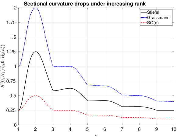
Figure 1: (Corresponding to Section 4.1.) Sectional curvature on $SO(20)$, $St(20,10)$, $Gr(20,10)$ for the tangent sections defined by (24). In all cases, the respective global sectional curvature maximum is attained for the matrices with subblocks $B_{1}$, $B_{2}$ as stated in Theorem Theorem.

The figure confirms that for the matrices under consideration, the global curvature maximum on all three manifolds is reached for tangent planes spanned by skew-symmetric $X,Y$ that feature zero diagonal blocks and the rank-two off-diagonal subblocks $B_{1},B_{2}$ from (22).

4.2 Experiment 2: Curvature associated with pseudo-random sections

Next, we run an experiment with random-matrices of increasing dimension. To this end, we create random skew-symmetric matrices

$$X(A_{1},B_{1},C_{1})=\begin{pmatrix}A_{1}&-B_{1}^{T}\\ B_{1}&C_{1}\end{pmatrix},\quad Y(A_{2},B_{2},C_{2})=\begin{pmatrix}A_{2}&-B_{2}^{T}\\ B_{2}&C_{2}\end{pmatrix}\in\operatorname{skew}(2p).$$

We start from $p=2$. For each $p=2,\ldots,1000$, a number of $100$ random pairs $X,Y\in\operatorname{skew}(2p)$ are computed and the sectional curvature of the tangent plane spanned by $X,Y\in T_{I}SO(2p)$, the tangent plane spanned by $X_{\mathfrak{m}^{St}}=X(A_{1},B_{1},\mathbf{0}),Y_{\mathfrak{m}^{St}}=Y(A_{2},B_{2},\mathbf{0})\in T_{[I]}St(2p,p)$ and the tangent plane spanned by $X_{\mathfrak{m}^{Gr}}=X(\mathbf{0},B_{1},\mathbf{0})$, $Y_{\mathfrak{m}^{Gr}}=Y(\mathbf{0},B_{2},\mathbf{0}),\in T_{[I]}Gr(2p,p)$, respectively, is computed. The result is then averaged over the number of random runs. Figure 2 displays the sectional curvature versus the block dimension $p$ on a logarithmic scale. It can be seen that the curvature of these ”random” planes is largest for $p=2$ and drops considerably, when $p$ is increased. To be precise, for the Stiefel data, the averaged random curvature at $p=2$ is $K=0.353$, while it is $K=8.81\cdot 10^{-3}$ for $p=100$ and $K=8.88\cdot 10^{-4}$ for $p=1000$.

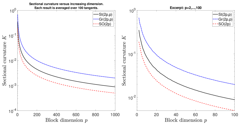
Figure 2: (Corresponding to Section 4.2.) Averaged sectional curvature for random tangent sections $X=X(A_{1},B_{1},C_{1}),Y=Y(A_{2},B_{2},C_{2})\in\operatorname{skew}(2p)$. The dimension of the subblocks is $p$. For Grassmann and Stiefel, $X,Y$ are projected onto the respective horizontal space.

4.3 Experiment 3: Impact of the blocks A and B

Consider the special matrices

$$A_{1} =\begin{pmatrix}[cccc]0&1&0&0\\ -1&0&0&0\\ 0&0&0&1\\ 0&0&-1&0\end{pmatrix},\quad A_{2}=\begin{pmatrix}[cccc]0&0&0&1\\ 0&0&1&0\\ 0&-1&0&0\\ -1&0&0&0\end{pmatrix}$$

$$B_{1}(u,v) =\begin{pmatrix}[cccc]0&1&0&0\\ -1&0&0&0\\ 0&0&0&u\\ 0&0&-v&0\end{pmatrix},\quad B_{2}(u,v)=\begin{pmatrix}[cccc]1&0&0&0\\ 0&1&0&0\\ 0&0&u&0\\ 0&0&0&v\end{pmatrix}$$

The matrix pair $A_{1},A_{2}$ maximizes the commutator norm $\|[A_{1},A_{2}]\|_{F}$, for $(u,v)=(0,0)$, the matrix pair $B_{1},B_{2}$ makes the Wu-Chen inequality sharp. Let

$$K^{St}(A_{1},B_{1},A_{2},B_{2}):=K^{St}(\begin{pmatrix}A_{1}&-B_{1}^{T}\\ B_{1}&\mathbf{0}\end{pmatrix},\begin{pmatrix}A_{2}&-B_{2}^{T}\\ B_{2}&\mathbf{0}\end{pmatrix}).$$

Figure 3 (left) displays the function

$$[0,1]^{2}\to\mathbb{R},(u,v)\mapsto K^{St}(\mathbf{0},B_{1}(u,v),\mathbf{0},B_{2}(u,v)).$$

Figure 3 (right) displays the function

$$[0,1]\to\mathbb{R},u\mapsto K^{St}(uA_{1},(1-u)B_{1}(0,0),uA_{2},(1-u)B_{2}(0,0)).$$

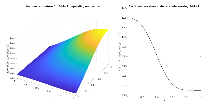
Figure 3: Sectional curvature on Stiefel.

5 Summary

This paper resumes the investigation of the sectional curvature on the Stiefel and Grassmann manifolds. In the Grassmann case, tight bounds have been known since the work if Wong [29] from 1968. We pay special attention to the maximizers of the curvature bounds and provide refined matrix trace inequalities for this purpose.

An extensive study of the sectional curvature on the Stiefel manifold equipped with a parametric family of Riemannian metrics has been conducted in [20]. However, since the formulae apply to all members of the family, it can be tedious to extract specific formulae for a particular metric. Moreover, tight bounds were only obtained for Stiefel manifolds $St(n,p)$ with $p=2$.

Under the canonical metric, which is a member of the parametric family, we confirm prior conjectures regarding the sectional curvature. Specifically, we establish that the curvature on the Stiefel manifold equipped with this metric globally does not exceed 5/4. With this addition, we now have a complete account of the curvature bounds in all admissible dimensions.

We also show that the sections that maximise the Grassmann curvature are exactly those for which the Stiefel curvature is maximised, and that these tangent space sections are necessarily spanned by special rank-two matrices. This supports the observation that ’high curvature means low-rank’, which is illustrated by numerical experiments that reveal a decrease in curvature with increasing the rank.

Appendix A The global maximum of the curvature bound of (21)

We formally verify that the function in (21) that bounds the sectional curvature of the Stiefel manifold

(25) $$\tilde{f}:(\alpha_{1},\alpha_{2})\mapsto\frac{5}{4}+\frac{5}{16}\alpha_{1}^{2}\alpha_{2}^{2}-\frac{1}{2}(\alpha_{1}^{2}+\alpha_{2}^{2})+\frac{1+\sqrt{2}}{4}\alpha_{1}\alpha_{2}\sqrt{1-\frac{1}{2}\alpha_{1}^{2}}\sqrt{1-\frac{1}{2}\alpha_{2}^{2}}$$

has its global maximum at $(0,0)$ for $(\alpha_{1},\alpha_{2})\in\left[0,\sqrt{2}\right]^{2}$.
Consider the transformation $\alpha:\left[0,\frac{\pi}{2}\right]\to\left[0,\sqrt{2}\right],r\mapsto\alpha(r)=\sqrt{2}\sin{(r)}$ so that $\sqrt{1-\frac{1}{2}\alpha^{2}}=\cos{(r)}$ and

$$\alpha\sqrt{1-\frac{1}{2}\alpha^{2}}=\sqrt{2}\sin{(r)}\cos{(r)}=\frac{\sqrt{2}}{2}\sin{(2r)}.$$

With parameterizing $\alpha_{1}=\alpha_{1}(r),\alpha_{2}=\alpha_{2}(s)$ in this form, the task is equivalent to showing that the global maximum of $f(r,s):=\tilde{f}(\alpha_{1}(r),\alpha_{2}(s))$,

$$f(r,s)=\frac{5}{4}+\frac{5}{4}\sin(r)^{2}\sin(s)^{2}-\sin(r)^{2}-\sin(s)^{2}+\frac{1+\sqrt{2}}{8}\sin(2r)\sin(2s),$$

in the admissible range $\left[0,\frac{\pi}{2}\right]^{2}$ is at $(0,0)$. The gradient of $f$ is

$$\nabla f(r,s)=\begin{bmatrix}f_{r}(r,s)\\ f_{s}(r,s)\end{bmatrix}=\begin{bmatrix}\frac{1}{2}\sin(r)\cos(r)\left(5\sin(s)^{2}-4\right)+\frac{1+\sqrt{2}}{4}\cos(2r)\sin(2s)\\ \frac{1}{2}\sin(s)\cos(s)\left(5\sin(r)^{2}-4\right)+\frac{1+\sqrt{2}}{4}\cos(2s)\sin(2r)\end{bmatrix}.$$

The condition $f_{r}(r,s)=0$ gives

(26) $$\frac{1}{2}\sin(r)\cos(r)\left(4-5\sin(s)^{2}\right)=\frac{1+\sqrt{2}}{4}\cos(2r)\sin(2s).$$

We assume $r,s\neq\frac{\pi}{4}$ and $\sin(s)^{2},\sin(r)^{2}\neq\frac{4}{5}$ and tackle those special cases afterwards. With excluding those cases we equivalently obtain

(27) $$\frac{1}{2}\frac{\sin(r)\cos(r)}{\cos(2r)}=\frac{1+\sqrt{2}}{4}\frac{\sin(2s)}{4-5\sin(s)^{2}}.$$

The left-hand side is greater than zero for $r<\frac{\pi}{4}$ and smaller than zero for $r>\frac{\pi}{4}$ and in each case monotonically increasing. The same holds for the right-hand side with $\sin(s)^{2}<\frac{4}{5}$ and $\sin(s)^{2}>\frac{4}{5}$. We only consider the case where both sides are greater than zero. The other cases can be tackled analogously. Due to the monotonicity of both sides, it immediately follows that there is at most one pair $(r,s)$ that fulfills the equation. Suppose $(r,s)$ is a pair satisfying the equation. We will show that in this case $r$ has to be equal to $s$. Assume $r\neq s$. Let $s<r<\frac{\pi}{4}$ and investigate $f_{s}(r,s)=0$ which is equivalent to

(28) $$\frac{1}{2}\frac{\sin(s)\cos(s)}{\cos(2s)}=\frac{1+\sqrt{2}}{4}\frac{\sin(2r)}{4-5\sin(r)^{2}}.$$

With $s<\frac{\pi}{4}$ we are also in the case where both sides have to be positive in order for the equation to hold. The equation (28) for $f_{s}$ is the same as the equation (27) for $f_{r}$, but with the roles for $r$ and $s$ reversed. Thus, for the pair $(r,s)$ fulfilling the equation (28), $r<s$ applies. This contradicts the above assumption. The case $r<s$ can be tackled in the same way. In summary, for the equation to hold, $r$ must be equal to $s$ so that candidates for extrema lie necessarily on the diagonal $r=s$. Along this diagonal, the function $\eqref{eq:globmax}$ bounding the sectional curvature becomes a parabola in $\alpha^{2}$

$$\tilde{f}:\alpha\mapsto\frac{5}{4}+\frac{3-2\sqrt{2}}{16}\alpha^{4}-\frac{3-\sqrt{2}}{4}\alpha^{2}.$$

It is easy to show that $\tilde{f}$ is monotonically strictly decreasing for $\alpha\in\left[0,\sqrt{2}\right]$ and therefore the maximum is at $\alpha=0$.
Now, we tackle the remaining cases $r,s=\frac{\pi}{4}$ and $\sin(s)^{2},\sin(r)^{2}=\frac{4}{5}$. At $r=\frac{\pi}{4}$, the condition $f_{r}(r,s)=0$ yields $\sin(s)^{2}=\frac{4}{5}$. But in this case $f_{s}(r,s)\neq 0$. The other combinations can be treated analogously (and are also not describing any extreme points). This completes the analysis and verifies that $\tilde{f}$ has its unique global maximum in the admissible range $\left[0,\sqrt{2}\right]^{2}$ at $(0,0)$. Figure 4 displays the function $\tilde{f}$.

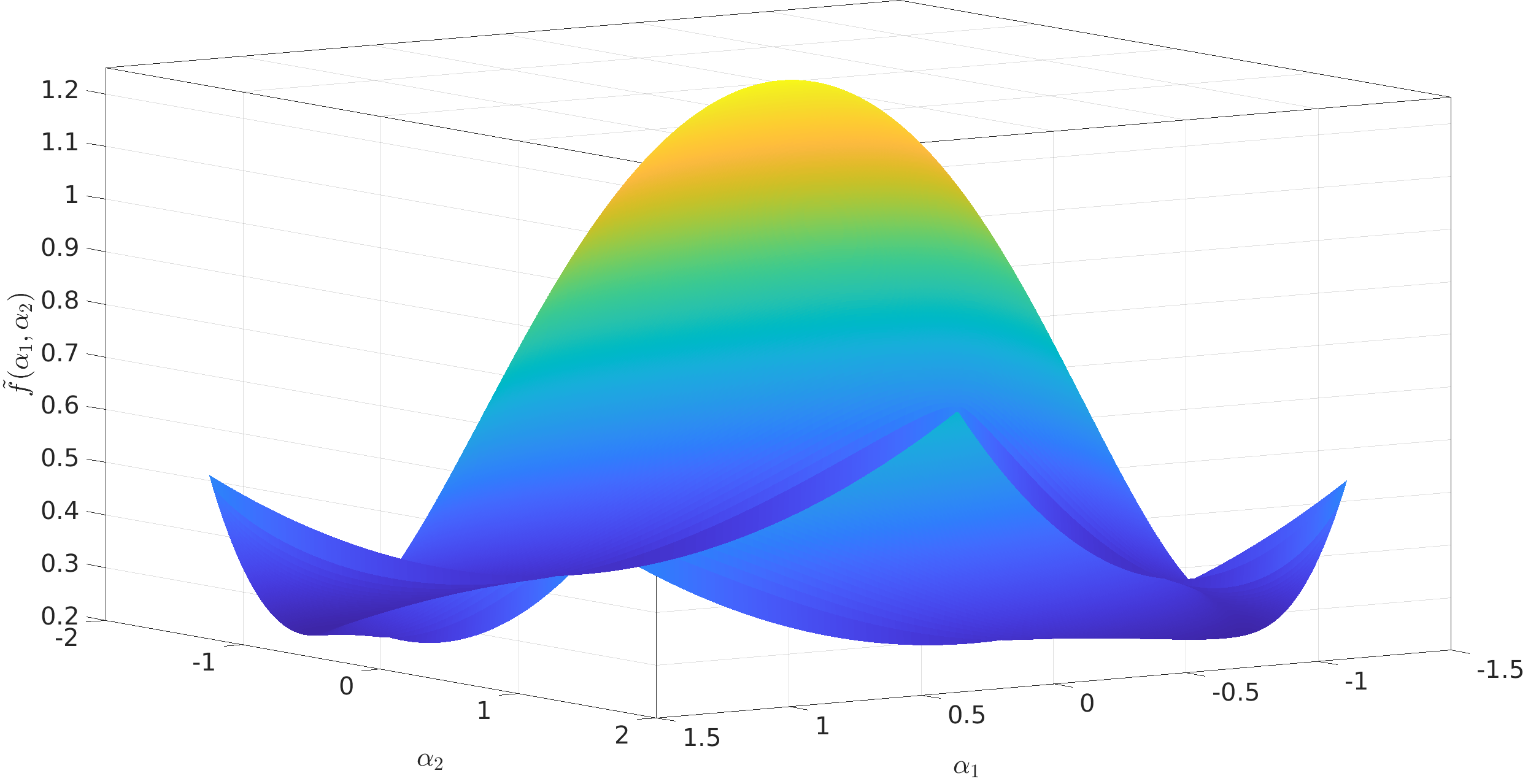
Figure 4: Plot of the function $\tilde{f}$ from (25) that bounds the Stiefel sectional curvature in the range $[-\sqrt{2},\sqrt{2}]^{2}$.

Appendix B The sectional curvature of special $St(n,p)$

For the sake of completeness, we give a direct proof of item 4 of Theorem Theorem:

On $St(3,2)$ and $St(3,3)$, the sectional curvature is $K^{St}(X,Y)\equiv\frac{1}{4}.$

The result is already contained in [20, Prop. 6.1]. It follows also immediately from Remark Remark combined with (19).

Proof.

On $St(3,2)$, tangent vectors are skew-symmetric $(3\times 3)$-matrices,

$$X=\begin{pmatrix}A&-B^{T}\\ B&\mathbf{0}\end{pmatrix}=\begin{pmatrix}[cc|c]0&-a&-b_{1}\\ a&0&-b_{2}\\ \hline\cr b_{1}&b_{2}&0\end{pmatrix}.$$

For $X\in\operatorname{skew}(3)$ as above, let $x:=\text{vec}_{3}(X)=(a,b_{1},b_{2})\in\mathbb{R}^{3}$ be the vector that features the independent entries of $X$ as components. Let $X,Y\in\operatorname{skew}(3)$ and $x=\text{vec}_{3}(X)$, $y=\text{vec}_{3}(Y)$. The following facts are well-known and may be verified by elementary means:

• $\text{vec}_{3}([X,Y])=x\times y$.

• $\langle X,Y\rangle_{F}=2\langle x,y\rangle_{2}$. In particular, $\|X\|_{F}^{2}=2\|x\|_{2}^{2}$ and $(X\bot_{F}Y)\Leftrightarrow(x\bot_{F}y)$.

Let $X,Y\in\operatorname{skew}(3)$ be an ONB w.r.t. the Frobenius inner product. In this case, $\|x\|_{2}=\frac{1}{\sqrt{2}}=\|y\|_{2}$ for the associated vector representations. The curvature formula of Remark Remark applies and gives

$$K(X,Y)=\frac{1}{2}\|[X,Y]\|_{F}^{2}=\frac{1}{2}2\|x\times y\|_{2}^{2}=\|x\|_{2}^{2}\|y\|_{2}^{2}\left\|\frac{x}{\|x\|_{2}}\times\frac{y}{\|y\|_{2}}\right\|_{2}^{2}=\frac{1}{4}.$$

The same reasoning applies to $St(3,3)$.

Note that with the tools at hand, (19) is a one-liner,

$$\|[X,Y]\|_{F}^{2}=2\|x\times y\|_{2}^{2}\leq 2\|x\|_{2}^{2}\|y\|_{2}^{2}=2\frac{1}{2}\|X\|_{F}^{2}\frac{1}{2}\|Y\|_{F}^{2}=\frac{1}{2}\|X\|_{F}^{2}\|Y\|_{F}^{2}.$$

Equality holds if and only if $X\bot_{F}Y$.

Appendix C Lie group essentials

This section recaps the basics of Lie groups and quotients of Lie groups. It is mainly collected from the textbooks [9], [14] and [21].

C.1 Matrix Lie groups

A Lie group is a differentiable manifold $\mathcal{G}$ which also has a group structure, such that the group operations ‘multiplication’ and ‘inversion’,

$$\mathcal{G}\times\mathcal{G}\ni(g,\tilde{g})\mapsto g\cdot\tilde{g}\in\mathcal{G}\mbox{\hskip 2.84544pt and }\hskip 2.84544pt\mathcal{G}\ni g\mapsto g^{-1}\in\mathcal{G}$$

are both smooth. By definition, a matrix Lie group $\mathcal{G}$ is a subgroup of $GL(n,\mathbb{C})$ that is closed relative to $GL(n,\mathbb{C})$. It is then also a Lie group in the above sense.

Let $\mathcal{G}$ be a real matrix Lie group. When endowed with the bracket operator or matrix commutator $[X,Y]=XY-YX$, the tangent space $T_{I}\mathcal{G}$ at the identity is the Lie algebra associated with the Lie group $\mathcal{G}$ and is denoted by $\mathfrak{g}=T_{I}\mathcal{G}$. The linear, skew-symmetric bracket operation is called Lie bracket and satisfies the Jacobi identity

$$[X,[Y,Z]]+[Z,[X,Y]]+[Y,[Z,X]]=0.$$

For any $A\in\mathcal{G}$, the function “left-multiplication with $A$” is a diffeomorphism $L_{A}:\mathcal{G}\to\mathcal{G},L_{A}(B)=AB$; its differential at a point $B\in\mathcal{G}$ is the isomporphism

$$d(L_{A})_{B}:T_{B}\mathcal{G}\to T_{L_{A}(B)}\mathcal{G},\quad d(L_{A})_{B}(X)=AX.$$

(Analogous for “right-multiplication with $A$”, $R_{A}(B)=BA$, $d(R_{A})_{B}(X)=XA$.) The tangent space at an arbitrary location $A\in\mathcal{G}$ is given by the translates (by left-multiplication) of the tangent space at the identity:

(29) $$T_{A}\mathcal{G}=T_{L_{A}(I)}\mathcal{G}=A\mathfrak{g}=\left\{\Delta=AX\in\mathbb{R}^{n\times n}|\hskip 5.69046ptX\in\mathfrak{g}\right\},$$

[12, §5.6, p. 160]. The Lie algebra $\mathfrak{g}=T_{I}\mathcal{G}$ of $\mathcal{G}$ can equivalently be characterized as the set of all matrices $\Delta$ such that $\exp_{m}(t\Delta)\in\mathcal{G}$ for all $t\in\mathbb{R}$, see [14, Def. 3.18 & Cor. 3.46] for the details. The exponential map for a matrix Lie group is the matrix exponential restricted to the corresponding Lie algebra [14, §3.7],

$$\exp_{m}|_{\mathfrak{g}}:\mathfrak{g}\rightarrow\mathcal{G}.$$

A Riemannian metric $\langle\cdot,\cdot\rangle_{g}^{\mathcal{G}}$ on $\mathcal{G}$ is called left-invariant if

$$\langle d(L_{A})_{B}X,d(L_{A})_{B}Y\rangle_{AB}^{\mathcal{G}}(=\langle AX,AY\rangle_{AB}^{\mathcal{G}})=\langle X,Y\rangle_{B}^{\mathcal{G}}$$

for all $X,Y\in T_{B}\mathcal{G}$. It is called right-invariant, if

$$\langle d(R_{A})_{B}X,d(R_{A})_{B}Y\rangle_{BA}^{\mathcal{G}}(=\langle XA,YA\rangle_{BA}^{\mathcal{G}})=\langle X,Y\rangle_{B}^{\mathcal{G}}$$

for all $X,Y\in T_{B}\mathcal{G}$. If a metric is left- and right-invariant, it is called bi-invariant.

C.2 Quotients of Lie groups by closed subgroups

Let $\mathcal{G}$ be a Lie group and $\mathcal{H}\leq\mathcal{G}$ be a Lie subgroup. For $A\in\mathcal{G}$, a subset of $\mathcal{G}$ of the form $[A]:=A\mathcal{H}=\{A\cdot Q|\hskip 2.84544ptQ\in\mathcal{H}\}$ is called a left coset of $\mathcal{H}$. The left coset $[I]$ is the subgroup itself. The left cosets form a partition of $\mathcal{G}$, and the quotient space $\mathcal{G}/\mathcal{H}$ determined by this partition is called the left coset space of $\mathcal{G}$ modulo $\mathcal{H}$, see [17, §21, p. 551]. The next is the central theorem for quotients of Lie groups.

Theorem.

(cf. [17, Thm 21.17, p. 551]) Let $\mathcal{G}$ be a Lie group and let $\mathcal{H}$ be a closed subgroup of $\mathcal{G}$. The left coset space $\mathcal{G}/\mathcal{H}$ is a manifold of dimension $\dim\mathcal{G}-\dim\mathcal{H}$ with a unique differentiable structure such that the quotient map $\pi:\mathcal{G}\to\mathcal{G}/\mathcal{H},A\mapsto[A]$ is a smooth surjective submersion. The left action of $\mathcal{G}$ on $\mathcal{G}/\mathcal{H}$ given by $A(B\mathcal{H})=(AB)\mathcal{H}$ turns $\mathcal{G}/\mathcal{H}$ into a homogeneous $\mathcal{G}$-space.

Each preimage $\mathcal{G}_{\pi(A)}:=\pi^{-1}([A])\subset\mathcal{G}$, called fiber, is a closed, embedded submanifold. Under the Riemannian metric $\langle\cdot,\cdot\rangle_{A}^{\mathcal{G}}$, at each point $A\in\mathcal{G}$, the tangent space $T_{A}\mathcal{G}$ decomposes into an orthogonal direct sum $T_{A}\mathcal{G}=T_{A}\mathcal{G}_{\pi(A)}\oplus(T_{A}\mathcal{G}_{\pi(A)})^{\bot}$ with respect to the metric. The tangent space of the fiber $T_{A}\mathcal{G}_{\pi(A)}=:V_{A}$ is the kernel of the differential $d\pi_{A}:T_{A}\mathcal{G}\to T_{\pi(A)}\mathcal{G}/\mathcal{H}$ and is called the vertical space. Its orthogonal complement $H_{A}:=V_{A}^{\bot}$ is the horizontal space. The key issue is that the tangent space of the quotient at $[A]=\pi(A)$ may be identified with the horizontal space at $A$.

$$H_{A}\cong T_{[A]}\mathcal{G}/\mathcal{H}.$$

• For every tangent vector $Y\in T_{[A]}(\mathcal{G}/\mathcal{H})$ there is $\bar{Z}=\bar{X}+\bar{Y}\in V_{A}\oplus H_{A}=T_{A}\mathcal{G}$ such that $d\pi_{A}(\bar{Z})=Y$. The horizontal component $\bar{Y}\in H_{A}$ is unique and is called the horizontal lift of $Y\in T_{\pi(A)}(\mathcal{G}/\mathcal{H})$. By going to the horizontal lifts, a Riemannian metric on the quotient can be defined by

  (30) $$\langle Y_{1},Y_{2}\rangle_{[A]}^{\mathcal{G}/\mathcal{H}}:=\langle\bar{Y}_{1},\bar{Y}_{2}\rangle_{A}^{\mathcal{G}}$$

  for $Y_{1},Y_{2}\in T_{[A])}(\mathcal{G}/\mathcal{H})$.

• W.r.t. this (and only this) metric, by construction, $d\pi_{A}$ preserves inner products: $d\pi_{A}$ is a linear isometry between $H_{A}$ and $T_{[A]}(\mathcal{G}/\mathcal{H})$.

• Horizontal geodesics in $\mathcal{G}$ are mapped to geodesics in $\mathcal{G}/\mathcal{H}$ under $\pi$. Horizontal geodesics are geodesics with velocity field staying in the horizontal space for all time $t$.

At the special point $A=I$, the vertical space is the Lie algebra of $\mathcal{H}$, $V_{I}=\ker{d\pi_{I}}=\mathfrak{h}$. This is because $\mathcal{H}=\pi^{-1}(I)$. For any curve $C(t)\subset\pi^{-1}(I)=\mathcal{H}$ starting from $C(0)=I$ with image in the fiber, it holds $\dot{C}(0)\in T_{I}\mathcal{H}=\mathfrak{h}$. On the other hand, $\pi$ is constant along the fiber so that $0=\frac{d}{dt}\big{|}_{t=0}\pi(C(t))=d\pi_{I}[\dot{C}(0)]$. Hence, any vector tangent to $\mathcal{H}$ at $I$ is in the kernel of $d\pi_{I}$. At the identity $I$, the splitting into vertical and horizontal space is

$$T_{I}\mathcal{G}=\mathfrak{h}\oplus\mathfrak{m}=V_{I}\oplus H_{I}=T_{I}\mathcal{H}\oplus(T_{I}\mathcal{H})^{\bot}.$$

Hence, the tangent space of the quotient at $\pi(I)$ is $\mathfrak{m}\cong T_{\pi(I)}\mathcal{G}/\mathcal{H}$. This choice of symbols is common in the literature, but the reader should be aware that $\mathfrak{h}$ is the vertical space, with the choice of letter referring to the subgroup name $\mathcal{H}$ and not to ”h for horizontal”. The choice of the symbol $\mathfrak{m}$ is motivated by the fact that if the quotient space is called $\mathcal{M}:=\mathcal{G}/\mathcal{H}$, then $\mathfrak{m}$ is the tangent space at $\pi(I)$. It is not the associated Lie algebra though, because in general $\mathcal{G}/\mathcal{H}$ is not a Lie group.

References

• [1] P.-A. Absil, R. Mahony, and R. Sepulchre. Riemannian geometry of Grassmann manifolds with a view on algorithmic computation. Acta Applicandae Mathematica, 80(2):199–220, 2004.
• [2] P.-A. Absil, R. Mahony, and R. Sepulchre. Optimization Algorithms on Matrix Manifolds. Princeton University Press, Princeton, New Jersey, 2008.
• [3] P. A. Absil and Simon Mataigne. The ultimate upper bound on the injectivity radius of the stiefel manifold, 2024.
• [4] D. Attali, H. Edelsbrunner, and Y. Mileyko. Weak witnesses for Delaunay triangulations of submanifolds. In B. Lévy and D. Manocha, editors, Proceedings of the 2007 ACM Symposium on Solid and Physical Modeling, Beijing, China, June 4-6, 2007, pages 143–150. ACM, 2007.
• [5] E. Begelfor and M. Werman. Affine invariance revisited. IEEE Conference on Computer Vision and Pattern Recognition, 2:2087–2094, 2006.
• [6] P. Benner, S. Gugercin, and K. Willcox. A survey of projection-based model reduction methods for parametric dynamical systems. SIAM Review, 57(4):483–531, 2015.
• [7] E. Celledoni, S. Eidnes, B. Owren, and T. Ringholm. Energy preserving methods on riemannian manifolds. Mathematics of Computation, 89:699–716, 2020.
• [8] A. Edelman, T. A. Arias, and S. T. Smith. The geometry of algorithms with orthogonality constraints. SIAM Journal on Matrix Analysis and Applications, 20(2):303–353, 1998.
• [9] J. Gallier and J. Quaintance. Differential Geometry and Lie Groups: A Computational Perspective. Geometry and Computing. Springer International Publishing, 2020.
• [10] K. A. Gallivan, A. Srivastava, X. Liu, and P. Van Dooren. Efficient algorithms for inferences on Grassmann manifolds. In IEEE Workshop on Statistical Signal Processing, pages 315–318, 2003.
• [11] J. Q. Ge. Ddvv-type inequality for skew-symmetric matrices and simons-type inequality for riemannian submersions. Advances in Mathematics, 251:62–86, 2014.
• [12] R. Godement and U. Ray. Introduction to the Theory of Lie Groups. Universitext. Springer International Publishing, 2017.
• [13] E. Hairer, C. Lubich, and G. Wanner. Geometric numerical integration: Structure-preserving algorithms for ordinary differential equations., volume 31 of Springer Series in Computational Mathematics. Springer-Verlag, Berlin, 2nd edition, 2006.
• [14] B. C. Hall. Lie Groups, Lie Algebras, and representations: An elementary introduction. Springer Graduate texts in Mathematics. Springer–Verlag, New York – Berlin – Heidelberg, 2nd edition, 2015.
• [15] K. Hüper, I. Markina, and F. Silva Leite. A Lagrangian approach to extremal curves on Stiefel manifolds. Journal of Geometrical Mechanics, 13(1):55–72, 2021.
• [16] A. Iserles, H. Z. Munthe-Kaas, S. P. Nørsett, and A. Zanna. Lie-group methods. Acta Numerica, 9:215–365, 2000.
• [17] J. M. Lee. Introduction to Smooth Manifolds. Graduate Texts in Mathematics. Springer New York, 2012.
• [18] Y. Man Lui. Advances in matrix manifolds for computer vision. Image and Vision Computing, 30(6–7):380–388, 2012.
• [19] H. Q. Minh and V. Murino. Algorithmic Advances in Riemannian Geometry and Applications: For Machine Learning, Computer Vision, Statistics, and Optimization. Advances in Computer Vision and Pattern Recognition. Springer International Publishing, Cham, 2016.
• [20] D. Nguyen. Curvatures of stiefel manifolds with deformation metrics. Journal of Lie Theory, 32(2):563–600, 2022.
• [21] B. O’Neill. Semi-Riemannian geometry - With applications to relativity, volume 103 of Pure and Applied Mathematics. Academic Press, New York, 1983.
• [22] V. Patrangenaru and L. Ellingson. Nonparametric Statistics on Manifolds and Their Applications to Object Data Analysis. Chapman & Hall/CRC Monographs on Statistics & Applied Probability. CRC Press, 2015.
• [23] P. Petersen. Riemannian Geometry. Graduate Texts in Mathematics. Springer International Publishing, 2016.
• [24] I. U. Rahman, I. Drori, V. C. Stodden, D. L. Donoho, and P. Schröder. Multiscale representations for manifold-valued data. SIAM Journal on Multiscale Modeling and Simulation, 4(4):1201–1232, 2005.
• [25] Q. Rentmeesters. Algorithms for data fitting on some common homogeneous spaces. PhD thesis, Université Catholique de Louvain, Louvain, Belgium, 2013.
• [26] A. Srivastava and P. K. Turaga. Riemannian computing in computer vision. Springer International Publishing, 2015.
• [27] S.-D. Wang, T.-S. Kuo, and C.-F. Hsu. Trace bounds on the solution of the algebraic matrix Riccati and Lyapunov equation. IEEE Transactions on Automatic Control, AC-31(7):654–656, 1986.
• [28] Y.-C. Wong. Differential geometry of Grassmann manifolds. Proceedings of the National Academy of Sciences of the United States of America, 57:589–594, 1967.
• [29] Y.-C. Wong. Sectional curvatures of Grassmann manifolds. Proceedings of the National Academy of Sciences of the United States of America, 60(1):75–79, 1968.
• [30] G. L. Wu and W. H. Chen. A matrix inequality and its geometric applications. Acta Math. Sinica, 31(3):348–355, 1988.
• [31] R. Zimmermann. Manifold interpolation. In P. Benner, S. Grivet-Talocia, A. Quarteroni, G. Rozza, W. Schilders, and L. M. Silveira, editors, System- and Data-Driven Methods and Algorithms, volume 1 of Model Order Reduction, pages 229–274. De Gruyter, Boston, 2021.
• [32] R. Zimmermann and K. Hüper. Computing the Riemannian logarithm on the Stiefel manifold: Metrics, methods, and performance. SIAM Journal on Matrix Analysis and Applications, 43(2):953–980, 2022.