ICLN: Input Convex Loss Network for Decision Focused Learning

Abstract

In decision-making problem under uncertainty, predicting unknown parameters is often considered independent of the optimization part. Decision-focused Learning (DFL) is a task-oriented framework to integrate prediction and optimization by adapting predictive model to give better decision for the corresponding task. Here, an inevitable challenge arises when computing gradients of the optimal decision with respect to the parameters. Existing researches cope this issue by smoothly reforming surrogate optimization or construct surrogate loss function that mimic task loss. However, they are applied to restricted optimization domain or build functions in a local manner leading a large computational time. In this paper, we propose Input Convex Loss Network (ICLN), a novel global surrogate loss which can be implemented in a general DFL paradigm. ICLN learns task loss via Input Convex Neural Networks which is guaranteed to be convex for some inputs, while keeping the global structure for the other inputs. This enables ICLN to admit general DFL through only a single surrogate loss without any sense for choosing appropriate parametric forms. We confirm effectiveness and flexibility of ICLN by evaluating our proposed model with three stochastic decision-making problems.

1 Introduction

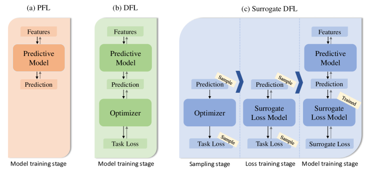
Figure 1: A model training pipeline for PFL, DFL and surrogate DFL. PFL trains predictive model by minimizing the prediction loss. DFL directly delivers gradients minimizing the task loss. Surrogate DFL first learns a surrogate loss model that follows the true task loss well by sampling predictions and its task losses. Then it trains the predictive model conveying useful gradients in an end-to-end manner.

Decision-making problem under uncertainty arise in various real-world applications such as production optimization, energy planning, or asset liability management (Shiina & Birge, 2003; Carino et al., 1994; Fleten & Kristoffersen, 2008; Delage & Ye, 2010; Garlappi et al., 2007). Such problems involve two main tasks: Prediction and Optimization. Prediction task aims to create model for uncertainty and estimate unknown parameters from some input features. This is often served by various machine learning (ML) techniques such as regression or deep learning. In Optimization task, corresponding optimization problem is solved with diverse off-the-shelf solver with estimated parameters from prediction task. For example in asset liability management, the asset returns are estimated in the prediction stage, and the optimal portfolio to repay the liability is obtained in the optimization stage based on the predictions.

The Prediction-Focused Learning (PFL) is the most commonly used framework to solve such problems, handling the two tasks in separate and independent steps. PFL first trains an ML model for the input features to yield predictions close to the observed parameters. Afterward, the decision-making problem is defined by the parameters predicted from trained ML model and solved to obtain an optimal decision. PFL is based on the underlying belief that accurate predictions will lead to good decisions. However, ML model frequently fails to achieve perfect accuracy, resulting a sub-optimal decision. Consequently, the prediction and optimization task are not distinct in many applications, but rather, they are intricately linked and should ideally be considered unitedly.

The Decision-focused Learning (DFL) achieves the above purpose by training ML model directly, seeking for predictions that result in good decisions. DFL combines prediction and optimization task by creating an end-to-end system that aims to decrease task loss. Task loss is defined as the quality of decisions obtained from a predictive model, and therefore depends on the optimal solution of the optimization problem. To learn a ML model, differentiating through the optimization problem is required to calculate the gradient of the task loss. This is a key challenge in the integration of prediction and optimization paradigm. However, the differentiation itself may be impossible because the decision variable is discrete or the objective function is discontinuous.

To address this challenge, various smooth surrogate optimization for DFL were proposed to obtain alternative gradient by forming relaxation of the original problem (Mandi et al., 2020; Wilder et al., 2019; Ferber et al., 2020) and adding regularization term to make the objective smooth (Amos et al., 2019; Wilder et al., 2019; Xie et al., 2020). While surrogate optimization still necessitates differentiation of the optimization problem, efforts have been made to develop solver-free surrogate loss functions that can effectively obtain gradients, referring as Surrogate DFL. Recent successful works of Surrogate DFL include SPO (Elmachtoub & Grigas, 2022), Contrasive Loss (Mulamba et al., 2020), LTR Loss (Mandi et al., 2022) and LODL (Shah et al., 2022). However, SPO, Contrasive loss and LTR loss are applied specifically to the linear objectives. While LODL can be implemented to general DFL problems, it creates and trains surrogate with specific parametric form for each data instance. Therefore, the time complexity is very large and the quality of the decision is greatly influenced by which parametric surrogate form is selected. The overall procedure of PFL, DFL and Surrogate DFL is illustrated in Figure 1.

In this paper, we propose Input Convex Loss Network (ICLN), which is a global and general surrogate loss for DFL. ICLN adopts Input Convex Neural Network (ICNN) (Amos et al., 2017) as a parametric surrogate form to approximate task loss. With ICNN, we can guarantee the surrogate loss function to be convex for some inputs, while maintaining general structure for the other inputs. Furthermore, users are not required to possess an artistic sense for selecting the suitable parametric function form for the task loss. Therefore, ICLN can handle the general DFL problems using only one surrogate loss, regardless of the number of observed data. We demonstrate the capability of ICLN on three stochastic decision-making problem, namely inventory stock problem, knapsack problem and portfolio optimization problem and show that ICLN learns task loss well with less time complexity.

2 Preliminaries

In this section, we motivate necessity of DFL approach from simple knapsack example. We also briefly summarize surrogate loss models and input convex neural networks.

Comparison on PFL and DFL       Prediction focused learning (PFL) and decision focused learning (DFL) are two big learning pipelines for the decision making problems under uncertainty as in Figure 1. Decision making problems can be considered in two big stages: model training stage and evaluation stage. We would like to focus on the model training stage. PFL learns the predictive model focusing on the prediction from the predictive model while DFL focuses on the objective (or task loss for minimization). Starting with PFL, the model training stage is again divided in two steps, prediction and optimization. In prediction step, PFL learns a predictive model by minimizing the prediction loss such as MSE. In optimization step, it solves a constrained optimization problem using the prediction of predictive model. By contrast, the predictive model in DFL is trained in an end-to-end manner. It focuses on learning the model to make good decisions (or actions), and therefore it uses task loss (or objective for maximization problem), rather than concentrating on minimizing the prediction loss.

To give a motivation in usage of DFL, we introduce a motivating example with a simple knapsack problem in Figure 2. Let’s consider two items: item 1 with value $40 and item 2 with $30 (true value, yellow star). Assume we can only select one item. Our objective is to predict the value of items by only observing the item features and choose one with a higher value. If we decide to choose item 1 (the optimal decision in this case), we would be happier, earning $40. Choosing item 2 is a sub-optimal decision, leading to a relative $10 loss. Suppose we predicted the values as blue dots and red crosses. In PFL point of view, the prediction loss of our prediction loss is equal to $20. Any prediction on the grey circle will give same prediction loss, which is not informative. In DFL standpoint, blue dots return zero task loss while red crosses gives task loss of $10. We show that minimizing the prediction loss may not lead to minimizing the task loss.

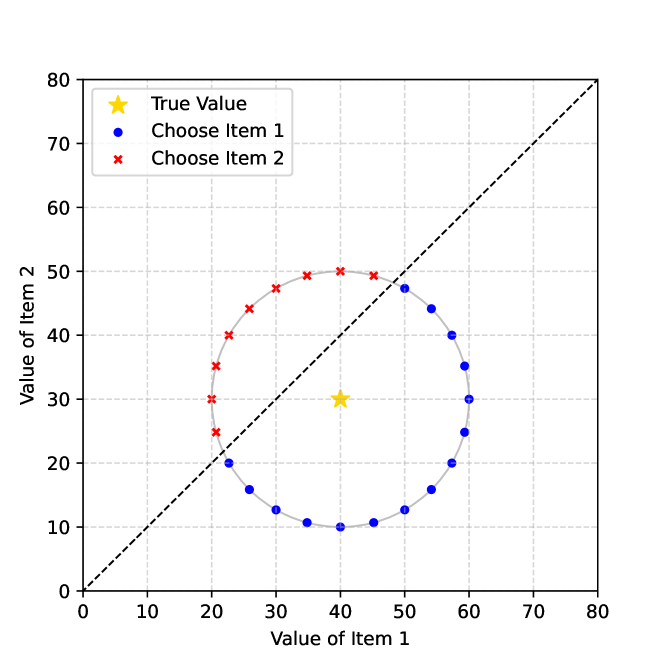
Figure 2: A simple example of knapsack problem. There are two items valued $40, $30 each. The true value of items is marked with yellow star. We predict the value of items and choose the higher one. Blue dots and red crosses are predicted values. PFL gives same prediction loss for every prediction while DFL gives $10 loss in red cross and 0 in blue.

Surrogate Loss Models       DFL compute task loss gradients with respect to the input parameters by for example, directly differentiating the optimization problem (or optimizer) (Donti et al., 2017). But in most of the general cases, the optimizer cannot be differentiated easily. To tackle this, methods using surrogate loss functions were proposed (Elmachtoub & Grigas, 2022). Surrogate loss models are differentiable and it approximates the mapping between the prediction and the task loss. As a consequence, it can be used to calculate the gradient to update the predictive model efficiently.

Input Convex Neural Networks       Amos et al. (2017) proposed Input Convex Neural Networks (ICNN) which is specific networks architecture to ensure convexity with respect to networks inputs. ICNN is constructed by introducing additional weights to connect input layer to each hidden layer. Given this structure, a non-decreasing convex activation functions such as ReLU and non-negativity of weights connecting between hidden layers are required to guarantee convexity of ICNN. The ICNN is categorized into Fully ICNN and Partial ICNN according to the size of the dimension for which convexity is maintained. ICLN uses both type of ICNN to show that it is possible to learn decision loss better than the existing local surrogate loss and expand it in a global manner.

3 Related Works

Various methodologies based on gradient based learning in DFL has been developed (Mandi et al., 2023). First, some approaches directly differentiated the constrained optimization problem to update the model parameters. (Donti et al., 2017) proposed an end-to-end pipeline tackling the stochastic optimization problems. They directly differentiated convex QPs with KKT optimality conditions and used Optnet (Amos & Kolter, 2017) for efficient differentiation. For general convex optimization problems, (Agrawal et al., 2019) proposed Cvxpylayers to differentiate the convex optimization problems. Alternatively, some works smoothened the optimization mapping by adding regularization terms. They added the Euclidean norm of the decision variables to use quadratic programming method (Wilder et al., 2019), or added the logarithmic barrier term to differentiate LP (Mandi & Guns, 2010). Furthermore, (Martins & Kreutzer, 2017) and (Amos et al., 2019) added the entropy term to solve for the multi-label problem. On the other hand, (Niepert et al., 2021) and (Berthet et al., 2020) tried to solve constrained optimization problem where the optimal solution is a random variable depending on the input parameters. Here, they used perturb-and-MAP (Papandreou & Yuille, 2011) framework to add regularization via perturbations.

Recent works on DFL showed tendencies on constructing a differentiable surrogate loss models. Smart ”Predict, Then Optimize” (SPO) (Elmachtoub & Grigas, 2022) proposed a convex SPO+ loss where the loss upper bounds the task loss. To update the predictive model, they obtained a subgradient of their proposed surrogate loss. NCE (Mulamba et al., 2020) used a noise contrastive approach (Gutmann & Hyvärinen, 2010) to build a family of surrogate loss for linear objectives. LTR (Mandi et al., 2022) applied this approach on ranking problems. SO-EBM (Kong et al., 2022) used an energy-based differentiable layer to model the conditional probability of the decision. The energy-based layer plays as a surrogate of the optimization problem. LODL (Shah et al., 2022) used supervised machine learning to locally construct surrogate loss models to represent task loss. They first sampled predictions near true instances for each instance and built a surrogate loss model respectively. They proposed three families for the model (e.g. WeightedMSE, Quadratic) to design a parametric surrogate loss models.

The key difference of our approach is (1) we do not need to handcraft for surrogate loss model, it is totally handcraft-free and (2) we additionally propose a global model to well represent true task loss, i.e. we suggest constructing a single model for task loss representation.

4 Input Convex Loss Network

Existing various optimization problems contain different task losses for each problem. For example, one could like to maximize the item value for the knapsack problem, while the other might want to minimize the risk in the portfolio optimization problem. However, designing a handcraft surrogate loss for each problem requires a lot of effort.

In this research, we would like to learn a task loss representation and construct a handcraft-free surrogate loss. First, we sample predictions and generate the prediction, task loss dataset. Here we obtain the decision on predictions using any optimization solver. With the generated dataset, we train a loss model to well represent the true task loss. Our goal is to learn a loss model that articulates a mapping from prediction to task loss. We propose two methods for the loss model; the local task loss representation ICLN-L, and global task loss representation ICLN-G, where we do not have to handcraft surrogate losses for each problem. Our models are a form of neural network, i.e. we can easily derive gradients to update the predictive model.

4.1 Learning Paradigm

First, we would like to define the objective regret that we would like to minimize. Given dataset $\mathcal{D}=\{(x_{i},y_{i})\}^{N}_{i=1}$ with $N$ instances, we can define regret as:

$$Regret\vcentcolon=\mathcal{L}_{task}(a^{*}(\hat{y}),y)-\mathcal{L}_{task}(a^{*}(y),y)$$

where $\mathcal{L}_{task}$ is a task loss defined for optimization problems, $y$ is the given true prediction, $\hat{y}$ is the prediction from the predictive model, and $a^{*}(\cdot)$ is an optimal action (or decision). Note that the task loss $\mathcal{L}_{task}$ is minimized for $\hat{y}=y$, inducing a zero regret. The optimal action is simply an output from the optimizer given the predictions, i.e.:

$$\hat{y} =\mathcal{M}_{\theta}(x)$$

$$a^{*}(\hat{y}) =\operatorname*{arg\,min}_{a\in\mathcal{A}}\mathcal{L}_{task}(a,\hat{y}).$$

where $\theta$ is the parameter of a predictive model $\mathcal{M}_{\theta}$, $x$ is the feature input for the predictive model and $\mathcal{A}$ is a set containing all possible outcomes from any optimization problem solver. Since the second term of the regret is nothing but a constant, minimizing the regret is equal to minimizing the task loss for a given dataset:

$$\operatorname*{min}_{\theta} \frac{1}{N}\sum_{i=1}^{N}\mathcal{L}_{task}(a^{*}(\hat{y_{i}}),y_{i})$$

s.t. $$a^{*}(\hat{y_{i}})=\operatorname*{arg\,min}_{a\in\mathcal{A}}\mathcal{L}_{task}(a,\mathcal{M}_{\theta}(x_{i})).$$

Next, the gradient minimizing the objective $\mathcal{L}_{task}$ for the update in model $\mathcal{M}_{\theta}$ can be obtained by differentiating with respect to the model parameter $\theta$ using a chain rule:

$$\frac{\partial\mathcal{L}_{task}}{\partial\theta} =\frac{\partial\mathcal{L}_{task}}{\partial a^{*}(\hat{y})}\cdot\frac{\partial a^{*}(\hat{y})}{\partial\hat{y}}\cdot\frac{\partial\hat{y}}{\partial\theta}$$ (1)

$$=\frac{\partial\mathcal{L}_{task}}{\partial\hat{y}}\cdot\frac{\partial\hat{y}}{\partial\theta}$$ (2)

$$\approx\frac{\partial\mathcal{L}_{surrogate}}{\partial\hat{y}}\cdot\frac{\partial\hat{y}}{\partial\theta}$$ (3)

where $\mathcal{L}_{surrogate}$ is a surrogate loss that we anticipate to learn.

Now, we desire to learn a mapping from prediction to loss by minimizing the difference between the task loss and the surrogate loss. To train the loss model via supervised machine learning, we first need to generate the prediction samples and its task loss using an optimizer. $K$ number of samples can be generated near the true prediction instance $y_{i}$ with adding a Gaussian noise for each component $j$ by:

$$\tilde{y}_{i,j}^{(k)}=y_{i,j}+c\cdot\mathcal{N}(0,1)$$ (4)

where $c$ is a factor controlling the sample variance. Then, our surrogate loss model can be trained as:

$$\psi^{*}=\operatorname*{arg\,min}_{\psi}\>\lVert\mathcal{L}_{\psi}(y)-\mathcal{L}_{task}(y,a^{*}(y))\rVert$$ (5)

where $\psi$ is a parameter of the surrogate loss model $\mathcal{L}_{\psi}$.

There are two perspectives for learning a loss model; a local, and a global perspective. Local perspective constructs the loss model for each prediction instance $y_{i}$, while global perspective builds a single model for task loss representation. We will show the details for each standpoint on Section 4.2 and 4.3.

What now remains is deriving a gradient $\frac{\partial\mathcal{L}_{\psi}}{\partial\hat{y}}$ to update the predictive model $\mathcal{M}_{\theta}$. Training $\mathcal{M}_{\theta}$ can be done easily with gradient descent, and therefore, it is crucial to build a loss model $\mathcal{L}_{\psi}$ to give informative gradients. For loss model to convey instructive gradients, we claim that $\mathcal{L}_{\psi}$ should be:

• Expressive: Good surrogate loss model should contain sufficient number of parameters to well approximate the true task loss. Lack in expressiveness may highly lead to under-performing loss models. With this approach, we take the idea of using a neural network.

• Easy to Differentiate: We need to differentiate our loss model with respect to $\hat{y}$ for gradients. Discontinuous or non-differentiable loss models will highly likely to suffer in such task. Therefore, we wish our model to be easily differentiable.

• Guaranteed in Convexity: Most importantly, we propose the loss model to be convex for every instance $y_{i}$. For the instance $y_{i}$ and its neighbor prediction samples $\tilde{y}_{i}^{(k)}$s, the task loss $\mathcal{L}_{task}(u,a^{*}(y_{i}))$ has a minimum when $u=y_{i}$. To extract informative gradient, we claim the surrogate loss model should also have a minimum at $y_{i}$, and therefore we want to guarantee convexity.

Gathering above approaches, we finally propose our input convex loss network (ICLN), a neural network that optimizes over the convex inputs to the network and outputs loss. ICLN uses input convex neural network (Amos et al., 2017) to learn surrogate loss convex to the inputs and contains sufficient number of parameters. Furthermore, ICLN is a convex in construction, and therefore is easy to differentiate; empirically, we can use a built-in backward functions to obtain gradients. During the following sections, we present ICLN-L and ICLN-G, the surrogate loss model in local and global perspective respectively.

Table 1: Results on three optimization problems with our methodologies ICLN-L, ICLN-G and benchmarks. Values represent mean and standard deviation of $\mathcal{L}_{relative}$ for test instances in a percentage(%) format. Lower the better. We bold-lettered the first and second lowest $\mathcal{L}_{relative}$ for each experiment. LODL was inapplicable on the inventory stock problem due to the absence of the true labels. For all three experiments, ICLN-L and ICLN-G showed the best performance compared to other benchmarks.

Problem	Methods
	PFL	DFL	LODL	NN	ICLN-L	ICLN-G
Inventory	12.76 (2.65)	10.03 (1.57)	- (-)	21.50 (2.55)	9.98 (1.17)	8.38 (4.28)
Knapsack	5.45 (8.25)	3.22 (8.10)	3.41 (8.71)	8.13 (8.35)	2.86 (7.73)	2.86 (6.89)
Portfolio	19.29 (12.46)	25.24 (9.23)	18.90 (8.59)	25.38 (13.03)	18.28 (2.38)	18.52 (1.46)

Table 2: Total number of samples required for training surrogate loss models on each experiment. ICLN-L used less samples compared to LODL and NN for learning loss. ICLN-G required the least samples for training, less than 0.01% size compared with LODL and NN in portfolio optimization problem.

Problem	Total Number of Samples
	LODL	NN	ICLN-L	ICLN-G
Inventory	-	20K	20K	4K
Knapsack	10M	10M	2M	100K
Portfolio	10M	10M	1M	0.6K

4.2 Local Task Loss Representation

We first introduce ICLN-L, the local input convex loss network that represents the task loss for each prediction instance $y_{i}$. Here, local means our ICLN-L is built for each prediction instance $y_{i}$. Each ICLN-L_i minimizes the task loss for the neighborhood of $y_{i}$. The trained loss model ICLN-L_i for instance $y_{i}$, $\mathcal{L}_{\psi_{i}}$, is later used to calculate the gradients for the prediction model $\mathcal{M}_{\theta}$ on an instance $(x_{i},y_{i})$.

To train the local surrogate loss $\mathcal{L}_{\psi_{i}}$ for instance $y_{i}$, we need a task loss dataset paired with predictions. First, we generate $K$ number of prediction samples near $y_{i}$. We use Equation (4) to sample predictions $\tilde{y}_{i}^{(k)}$. Next, we solve the optimization problem for each $\tilde{y}_{i}^{(k)}$ and obtain a dataset $\{(\tilde{y}_{i}^{(k)},\mathcal{L}_{task}(a(\tilde{y}_{i}^{(k)}),\tilde{y}_{i}^{(k)}))\}_{k=1}^{K_{L}}$. After that, we train our $\mathcal{L}_{\psi_{i}}$ by minimizing the mean squared error with the given task loss as in Equation (5).

Now that $\mathcal{L}_{\psi_{i}}$ has been trained for all $i\in N$, we train the predictive model $\mathcal{M}_{\theta}$ with the original instance dataset $\mathcal{D}=\{(x_{i},y_{i})\}^{N}_{i=1}$. We plug the training data $x_{i}$ to the untrained predictive model $\mathcal{M}_{\theta}$ and obtain prediction $\hat{y}_{i}=\mathcal{M}_{\theta}(x_{i}).$ Then, we derive the gradient for $\mathcal{M}_{\theta}$ by:

$$\frac{\partial\mathcal{L}_{task}(a^{*}(y_{i}),\hat{y}_{i})}{\partial\theta} \approx\frac{\partial\mathcal{L}_{\psi_{i}}(\hat{y}_{i})}{\partial\theta}$$ (6)

$$=\frac{\partial\mathcal{L}_{\psi_{i}}(\hat{y}_{i})}{\partial\hat{y}_{i}}\cdot\frac{\partial\hat{y}_{i}}{\partial\theta}$$ (7)

where $\mathcal{L}_{\psi_{i}}$ is our trained ICLN-L_i for instance $y_{i}$. Both $\frac{\partial\mathcal{L}_{\psi_{i}}(\hat{y}_{i})}{\partial\hat{y}_{i}}$ and $\frac{\partial\hat{y}_{i}}{\partial\theta}$ can be done easily by backpropagation. We have summarized our methodology for ICLN-L on Algorithm 1 in Appendix.

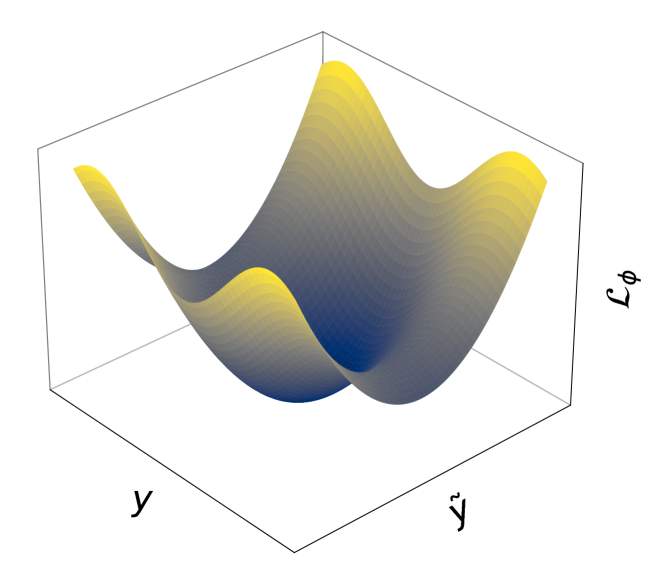
Figure 3: An intuitive illustration of ICLN-G mapping from $(y,\tilde{y})$ to $\mathcal{L}_{\phi}$. The loss function is convex in sampled neighbors $\tilde{y}$, but not in the instance $y$.

ICLN-L has its advantage since it represents local task loss by taking convex structure as a loss model for each instance and derives gradient easily. We once again emphasize that ICLN-L is a handcraft-free surrogate loss that automatically learns the mapping from prediction to task loss. We would also like to state that the sampling stage for constructing dataset $\{(\tilde{y}_{i}^{(k)},\mathcal{L}_{task}(a(\tilde{y}_{i}^{(k)}),\tilde{y}_{i}^{(k)}))\}_{k=1}^{K_{L}}$ is pre-processable, inferring that once we generate samples, we can use to build any number of predictive model $\mathcal{M}_{\theta}$ and other surrogate DFL models.

4.3 Global Task Loss Representation

While the local task loss representation well represents the true task loss, its inherent structure leads to increase in time complexity. As increase in number of instances, the time to train local loss models also proportionally increase. Therefore, here we propose a global task loss representation ICLN-G, that learns a mapping $(y_{i},\tilde{y}_{i}^{(k)})\rightarrow\mathcal{L}_{task}$.

Our key idea is to learn a loss model convex in instance neighborhood prediction samples $\tilde{y}_{i}^{(k)}$, but not necessarily convex in instance $y_{i}$. By leveraging our key idea, we retain the advantage to train our loss model to have a local minima at $y_{i}$ locally, while simultaneously learning a mapping from $y_{i}$s to task loss globally. We take the partial input convex neural network architecture (Amos et al., 2017) to guarantee convexity in $\tilde{y}_{i}^{(k)}$s, but not necessarily in $y_{i}$s. The architecture details of our loss model ICLN-G is available in Appendix.

To give an illustrative intuition of ICLN-G, $\mathcal{L}_{\phi}$, we prepared Figure 3. In a $\tilde{y}_{i}^{(k)}$ point of view, the loss $\mathcal{L}_{\phi}$ is convex. However, in a $y_{i}$ standpoint, the convexity is not guaranteed. Our goal is to learn such loss architecture maintaining the mentioned convexity characteristics.

The learning paradigm of ICLN-G, $\mathcal{L}_{\phi}$, is somewhat similar to learning $\mathcal{L}_{\psi_{i}}$s, but it has a crucial difference: we do not have to learn for each instance, we only learn a single loss model. First, we similarly generate prediction samples near true predictions for $\mathcal{L}_{\phi}$, but much less in size.

We generate $K_{G}$ number of samples in total to train the ICLN-G loss model. After training $\mathcal{L}_{\phi}$, we equivalently train $\mathcal{M}_{\theta}$ using the gradients calculated from $\mathcal{L}_{\phi}$, with slight changes in calculating gradient as:

$$\frac{\partial\mathcal{L}_{task}(a^{*}(y_{i}),\hat{y}_{i})}{\partial\theta} \approx\frac{\partial\mathcal{L}_{\phi}(y_{i},\hat{y}_{i})}{\partial\theta}$$ (8)

$$=\frac{\partial\mathcal{L}_{\phi}(y_{i},\hat{y}_{i})}{\partial(y_{i},\hat{y}_{i})}\cdot\frac{\partial(y_{i},\hat{y}_{i})}{\partial\theta}.$$ (9)

We have summarized our training paradigm with ICLN-G on Algorithm 2 in Appendix.

5 Experiments and Results

To show the performance of our proposed methodologies, we conduct three experiments with benchmarks. Codes for experiments are available at https://anonymous.4open.science/r/icln-7713/README.md

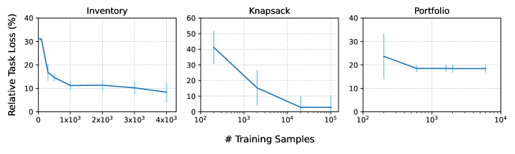
Figure 4: Relative Task Loss $\mathcal{L}_{relative}$ of ICLN-G for three experiments. Horizontal axis means the total number of training samples used for training ICLN-G. Knapsack and portfolio optimization problem is horizontally log-scaled. Connected dark-blue line represents mean $\mathcal{L}_{relative}$, light-blue line means standard deviation for each experiment. We claim ICLN-G converges to a sufficient performance relatively and remarkably smaller size in sample size compared to other benchmarks.

5.1 Problem Description

We selected three problems to tackle different situations. Inventory stock problem was chosen to show the methodologies may work even when the true instance is not available. The knapsack problem was selected to show the result of the motivation given on Section 2, where we anticipate PFL to not work well, but the DFL does. We picked the portfolio optimization problem as the last experiment to show performance in high dimension problems. We describe more details of the problem formulation and explanation below.

Inventory Stock Problem       In the inventory stock problem, we want to minimize the cost respect to the demand $y$ and order quantity $a$. The cost function is defined as:

$$f(y,a)=c_{0}a+\frac{1}{2}q_{0}a^{2}+c_{b}[y-a]_{+}+\frac{1}{2}q_{b}([y-a]_{+})^{2}\\ +c_{h}[a-y]_{+}+\frac{1}{2}q_{h}([a-y]_{+})^{2}.$$ (10)

To emphasize the model’s performance under uncertainty of the demand, we assumed that the demand is followed by the distribution conditioned on the observed features $x$. For the simplicity, we also assumed that the distribution of the demand is discrete. The input feature $x$ flows to the predictive model and outputs the probability vector for discrete demands. Then, the probability vector goes into an optimizer and outputs an optimal order quantity (which intuitively is similar to the expectation of the vector). Therefore, for the inventory stock problem, we predict the probability vector and optimize our ordering quantity. More details are provided in the appendix.

Knapsack Problem       To further extend the motivation between PFL and DFL, we test our methodologies on the Knapsack problem. The objective of the knapsack problem is to choose a set of items maximizing the value given a weight constraint where each item $i$ has a weight $w_{i}$ and value $y_{i}$. For our experiment, every item is assumed to have a same unit weight, i.e. the weight constraint implies the maximum number of items that one can choose. Thus, we predict the value $y_{i}$ for each item $i$ and optimize by choosing the set of largest valued items. The value $y_{i}$ of an item is induced from the underlying true distribution of $y$ where a feature vector $x$ is given as an input. We assume each element in the feature vector is distributed randomly in uniform: $x_{ik}\sim U(0,1)$ for every $k$. We let the number of features of a feature vector $k=2$ and the underlying true distribution $y_{i}=(x_{i1}-3x_{i1}^{2}x_{i2}-x_{i2})^{2}$ in our experiment.

Portfolio Optimization Problem       We test our methodologies on a higher domain. For $N$ =50 number of stocks, we would like to predict the future stock price $y$. Then, we optimize our action to ideally invest based upon the predicted prices to maximize profit with a risk regularization term. The optimization problem has a form of $\max_{a}\{\boldsymbol{y^{\top}a}-\gamma\cdot\boldsymbol{a^{\top}\Sigma a}:\sum_{i}\boldsymbol{a_{i}}=1\}$ where $\boldsymbol{a}\in\mathbb{R}^{N}$ is the weight vector we would like to invest (our action), $\Sigma\in\mathbb{R}^{N\times N}$ is the correlation matrix for $N$ stocks and $\gamma$ is the risk aversion factor.

5.2 Results

We first introduce our evaluation metric and benchmarks to compare among methodologies.

Evaluation Metric       We use relative task loss as the evaluation metric. Our relative task loss is better when lower. For minimization optimization problems as inventory stock problem, we denote model, optimal, worst task losses as $\mathcal{L}_{model}$, $\mathcal{L}_{opt}$, $\mathcal{L}_{worst}$ respectively. For maximization problems as knapsack and portfolio optimization problems, we use task objective to maximize and use the notation $\mathcal{V}$ as in value instead of $\mathcal{L}$. To normalize the metric to fall within the range of 0 to 1, we define the relative task loss slightly different for each problem: Since inventory stock problem is a minimization problem, we use the following metric:

$$\mathcal{L}_{relative}\vcentcolon=\frac{\mathcal{L}_{model}-\mathcal{L}_{opt}}{\mathcal{L}_{model}}.$$

Knapsack and portfolio optimization problem maximizes the total value of chosen items, and therefore we use:

$$\mathcal{L}_{relative}\vcentcolon=\frac{\mathcal{V}_{model}-\mathcal{V}_{worst}}{\mathcal{V}_{opt}-\mathcal{V}_{worst}}.$$

Note again that our $\mathcal{L}_{relative}$ is lower the better.

Benchmarks       We use 4 benchmarks to train the predictive model and compare with our ICLN-L and ICLN-G.

• PFL: For prediction focused learning (PFL), we use two-stage predict-then-optimize as a benchmark. It uses MSE or NLL loss to minimize prediction loss.

• DFL: Decision focused learning (DFL) provides gradient with back-propagating through differentiable optimizer.

• LODL: We used locally optimized decision loss (LODL) by (Shah et al., 2022), with the directed quadratic parametric loss model.

• NN: To show the importance of convexity, we use a simple dense neural network as a benchmark.

Table 1 presents the relative loss for each method on three experiments. The values are mean relative loss in percentage (%) with standard deviation inside the parenthesis. We tested 1000 instances for inventory stock problem and 400 instances for knapsack and portfolio optimization problem. We bold-lettered the first and second best results in mean. LODL was inapplicable in inventory stock problem since the true label did not exist due to the stochasticity. Both ICLN-L and ICLN-G show good performance both in mean and standard deviation perspective. From the poor performance of NN, we can imply that the convexity plays a critical role on learning the loss.

We presented the total sample size required for training each surrogate loss model on Table 2. $K,M$ stands for $10^{3},10^{6}$. The sample size required for training ICLN-L and ICLN-G was relatively smaller compared to LODL and NN. Surprisingly for portfolio optimization problem, ICLN-G required 600 samples, less than 0.01% of the sample size for training LODL, and out-performed (18.52 vs 18.90, lower the better).

To illustrate how $\mathcal{L}_{relative}$ changes as the number of training samples increases in ICLN-G, we tested for several sample sizes for each experiment in Figure 4. For each data point, we conducted experiments in an equivalent environment, only changing in a number of sample size. We discovered that ICLN-G approached to a decent performance with astonishingly small sample size.

Table 3: Time complexity for training loss models. We ignore the time for updating the predictive model, since it is identical everywhere. The total number of samples are $K\cdot N_{sol}$ for LODL, NN, ICLN-L and $K_{G}$ for ICLN-G. We emphasize that $K_{G}\ll K_{L}\cdot N_{sol}<K\cdot N_{sol}$ empirically.

Methods	Time Complexity
PFL	-
DFL	$\mathcal{O}(N_{sol}\cdot(T_{sol,F}+T_{sol,B}))$
LODL	$\mathcal{O}(K_{LODL}\cdot N_{sol}\cdot(T_{sol,F}+T_{LODL}))$
NN	$\mathcal{O}(K_{NN}\cdot N_{sol}\cdot(T_{sol,F}+T_{NN}))$
ICLN-L	$\mathcal{O}(K_{L}\cdot N_{sol}\cdot(T_{sol,F}+T_{L}))$
ICLN-G	$\mathcal{O}(K_{G}\cdot(T_{sol,F}+T_{G}))$

5.3 Time Complexities

Here we show the time complexity for deriving gradients for the model update.

• PFL: Since PFL directly minimizes with the loss metric (e.g. MSE) between $y$ and $\hat{y}$, the time spent on deriving a gradient on the model output is near zero.

• DFL: DFL also does not learn a loss function. Instead, it uses a differentiable solver for deriving a gradient. $N_{sol}$ represents the number of instances that an optimization problem needs to be solved. $T_{sol,F}$ and $T_{sol,B}$ means the forward, backward pass of the differentiable solver, respectively. To sum up, DFL method derives a gradient for the model by solving $N_{sol}$ number of optimization problems using the forward, backward pass of the solver model.

• LODL: LODL learns loss functions locally for every $N_{sol}$ instances and generates loss models for each instance. To learn a loss model, LODL generates $K$ number of samples for each instance and solves for the input of the model, i.e. solves $K_{LODL}\cdot N_{sol}$ optimization problems. After obtaining a dataset for the loss model, it forward and backward passes for training, consuming $T_{LODL}$.

• NN: For NN to learn, it requires $K_{NN}\cdot N_{sol}\cdot T_{sol,F}$ time for obtaining a dataset. Then, it forward and backward passes for training a dense neural network, taking $T_{NN}$ amount of time.

• ICLN-L: ICLN-L also learns local losses for every instances. It takes $K_{L}\cdot N_{sol}\cdot T_{sol,F}$ time for data generation and $T_{L}$ for training ICLN-L.

• ICLN-G: ICLN-G requires $K_{G}$ number of samples to train the single global model. For each sample, the time for solving the optimization problem $T_{sol,F}$ and training ICLN-G $T_{G}$ is required.

We state that the sampling stage in surrogate DFL methodologies are pre-processable and most importantly, parallelizable. Time consumption in sampling stage corresponds to the term containing $T_{sol,F}$. One can simply use 100 environments to solve 100 optimization problems in a single cycle. Considering that the sampling stage is totally parallelizable, we can even compare a small sample size requiring ICLN-G, consuming $K_{G}\cdot T_{G}$ (empirically fast), with PFL predict-then-optimize method.

6 Conclusion

In this paper, we proposed a methodology of learning a global surrogate loss model for decision focused learning. The model learns a mapping from prediction to the true task loss. To train the surrogate loss model, we first generate samples near true instances and train via supervised learning paradigm. The trained loss model is then used for deriving informative gradients for predictive model update. We constructed our surrogate loss ICLN using Input Convex Neural Network to guarantee convexity for specific inputs. We built the surrogate loss model in both local and global perspective: ICLN-L and ICLN-G. ICLN-L showed high performance on all three decision making problem, while ICLN-G also outperformed other benchmarks even though the model uses significantly less samples for training. With ICLN-G, we reduced the time complexity for training a ML model via DFL training pipeline. For future works, we look forward to develop a

Impact Statements

This paper presents work whose goal is to advance the field of Machine Learning. There are many potential societal consequences of our work, none which we feel must be specifically highlighted here.

Appendix A Input Convex Loss Network Details

A.1 Architecture Details

Here we show the architecture details of our Input Convex Loss Network (ICLN). The input is given as $(y_{i},\tilde{y}_{i})$ where $y_{i}$ is a given prediction instance and $\tilde{y}_{i}$ is a sampled prediction near $y_{i}$. We have colored bluish for convex vector flows and reddish for vectors flows that does not guarantee convexity. The dimension of hidden layers are written as a subscript inside parenthesis to easily recognize the dimension of each vectors. We drew linear layer in a trapezoid form if the dimension changes, and rectangle if it retains. The shaded linear layer has a constraint to have positive weights. Details for operators are available on Figure 5.

The left side of the figure shows the architecture from input to the first hidden layer. The right side presents how hidden layers are composed. The upstream of the right side is a flow for reddish vector representations, while the downside is for bluish vectors. For the output layer, one may may simply let $z_{i+1}$ as a output vector and ignore $u_{i+1}$.

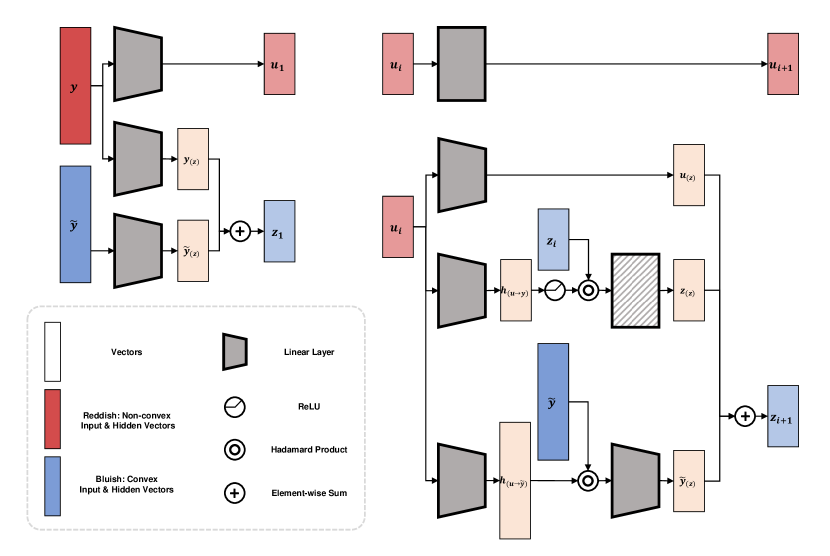
Figure 5: Architecture of Input Convex Loss Network. Left figure represents the input to the first hidden layer. The right figure shows the hidden to hidden layers for non-convex vectors (reddish, upstream) and convex vectors (bluish, downstream). Output layer can simply be considered as $z_{i+1}$ without $u_{i+1}$.

A.2 Algorithms

Here we show the algorithms for our model ICLN-L and ICLN-G. Note that ICLN-L loops for every instance $y_{i}$ while ICLN-G does not.

Algorithm 1 Train $\mathcal{M}_{\theta}$ with ICLN-L $\mathcal{L}_{\psi_{i}}$s (Local)

  Dataset: $\mathcal{D}=\{(x_{i},y_{i})\}^{N}_{i=1}$

  for $i=1$ to $N$ do

     1. Generate Dataset:

     for $k=1$ to $K_{L}$ do

        Sample $\tilde{y}_{i}^{(k)}\sim y_{i}+c\cdot\mathcal{N}(0,1)$

        Solve for $a^{*(k)}_{i}=\operatorname*{argmin}_{a}\mathcal{L}_{task}(a(y^{(k)}_{i}),\tilde{y}_{i}^{(k)})$ .

     end for

     Dataset $\{(\tilde{y}_{i}^{(k)},\mathcal{L}_{task}(a(\tilde{y}_{i}^{(k)}),\tilde{y}_{i}^{(k)}))\}_{k=1}^{K_{L}}$ built.

     2. Learn ICLN-L_is:

     Initialize $\mathcal{L}_{\psi_{i}}$.

     Learn $\mathcal{L}_{\psi_{i}}$ using Equation (5).

  end for

  3. Train Predictive Model $\mathcal{M}_{\theta}$:

  repeat

     Get predictive model prediction $\hat{y}_{i}=\mathcal{M}_{\theta}(x_{i})$.

     Train $\mathcal{M}_{\theta}$ using Equation (6) - (7).

  until Earlystopping

Algorithm 2 Train $\mathcal{M}_{\theta}$ with ICLN-G $\mathcal{L}_{\phi}$ (Global)

  Dataset: $\mathcal{D}=\{(x_{i},y_{i})\}^{N}_{i=1}$

  1. Generate Dataset:

  Sample $K_{G}$ samples near any instances $y_{i}$.

  for $k=1$ to $K_{G}$ do

     Solve for $a^{*(k)}_{i}=\operatorname*{argmin}_{a}\mathcal{L}_{task}(a(\tilde{y}_{i}^{(k)}),\tilde{y}_{i}^{(k)})$.

  end for

  Dataset $\{(\tilde{y}_{i}^{(k)},\mathcal{L}_{task}(a(\tilde{y}_{i}^{(k)}),\tilde{y}_{i}^{(k)}))\}_{k=1}^{K_{G}}$ built.

  2. Learn ICLN-G:

  Initialize $\mathcal{L}_{\phi}$.

  Learn $\mathcal{L}_{\phi}$ with Equation (5).

  3. Train Predictive Model $\mathcal{M}_{\theta}$:

  repeat

     Get predictive model prediction $\hat{y}_{i}=\mathcal{M}_{\theta}(x_{i})$.

     Train $\mathcal{M}_{\theta}$ using Equation (8) - (9).

  until Earlystopping

Appendix B Experiment Details

B.1 Details of Inventory Stock Problem

Expression       The cost function is defined as:

$$f(y,a)=c_{0}a+\frac{1}{2}q_{0}a^{2}+c_{b}[y-a]_{+}\frac{1}{2}q_{b}([y-a]_{+})^{2}+c_{h}[a-y]_{+}\frac{1}{2}q_{h}([a-y]_{+})^{2}$$ (11)

where our objective is to minimize the expectation of cost function:

$$\operatorname*{minimize}_{a}\quad\boldsymbol{E}_{y\sim p(y|x;\theta)}\left[f(y,a)\right].$$ (12)

By the discrete distribution assumption of demand $y$, we can rewrite the optimization problem as:

$$\operatorname*{minimize}_{a\in\mathbb{R}^{k},a_{b},a_{h}\in\mathbb{R}^{k}} c_{0}a+\frac{1}{2}q_{0}a^{2}+\sum_{i=1}^{k}\hat{y}_{i}\left(c_{b}(a_{b})_{i}+\frac{1}{2}q_{b}(a_{b})_{i}^{2}+c_{h}(a_{h})_{i}+\frac{1}{2}q_{h}(a_{h})_{i}^{2}\right)$$ (13)

subject to $$d-a\boldsymbol{1}\leq a_{b},\;\,a\boldsymbol{1}-d\leq a_{h},\;\,a,a_{h},a_{b}\geq 0.$$

where $\hat{y}_{i}\equiv p(y=d_{i}|x;\theta)$ for discrete demands $d_{1},\ldots,d_{k}$.

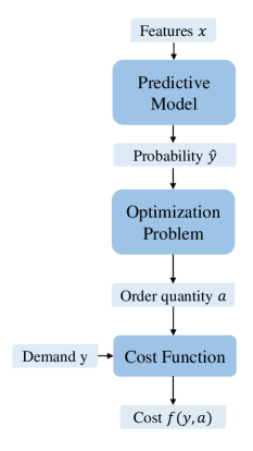
Figure 6: Process of Inventory Stock Problem. The objective is to minimize the cost

Experiment       We generate problem instances from randomly sampled $x\in\mathbb{R}^{n}$ with the distribution $p(y|x;\theta)\propto\text{exp}(\Theta^{\top}x)$ for the true parameter $\Theta\in\mathbb{R}^{n\times k}$
. We used 2000 pairs of $(x,y)$ for the train/validation set and 1000 pairs of $(x,y)$ for the test set.
The benchmark methods are 1) Two-stage learning using NLL Loss (PFL); 2) Task based learning model (Donti et al., 2017) (DFL); 3) Dense neural network (NN).

Sampling stage      Unlike normal LODL approach, Inventory stock problem does not have true probability label for each $(x,y)$ pair because of the stochasticity of demand. Therefore, we cannot construct loss models for each dataset. As an alternative, we created a loss model for each demand by grouping the datasets with demand. The main difficulty with this approach is that it is hard to generate samples for training each loss function. Hence, we sampled the total loss training dataset and the dataset was divided and labelled to each demand based on the expected value.

Loss Training stage       We trained surrogate loss with the sampled dataset.

• ICNN-L and NN : Each loss function for demand $i$ is trained with a dataset which label is $i$.
  # Loss training samples : 20000

• ICNN-G : The global loss function is trained with a labelled total dataset.
  # Loss training samples : 4000

Model training stage      We trained predictive model with the train dataset.

• ICNN-L and NN : Input of the surrogate loss function will be the output of predictive model.

• ICNN-G : Input of the surrogate loss function will be the data with output of predictive model and demand concatenated.

References

- Agrawal et al. (2019) Agrawal, A., Amos, B., Barratt, S., Boyd, S., Diamond, S., and Kolter, J. Z. Differentiable convex optimization layers. Advances in neural information processing systems, 32, 2019.
- Amos & Kolter (2017) Amos, B. and Kolter, J. Z. Optnet: Differentiable optimization as a layer in neural networks. In International Conference on Machine Learning, pp. 136–145. PMLR, 2017.
- Amos et al. (2017) Amos, B., Xu, L., and Kolter, J. Z. Input convex neural networks. In International Conference on Machine Learning, pp. 146–155. PMLR, 2017.
- Amos et al. (2019) Amos, B., Koltun, V., and Kolter, J. Z. The limited multi-label projection layer. arXiv preprint arXiv:1906.08707, 2019.
- Berthet et al. (2020) Berthet, Q., Blondel, M., Teboul, O., Cuturi, M., Vert, J.-P., and Bach, F. Learning with differentiable pertubed optimizers. Advances in neural information processing systems, 33:9508–9519, 2020.
- Carino et al. (1994) Carino, D. R., Kent, T., Myers, D. H., Stacy, C., Sylvanus, M., Turner, A. L., Watanabe, K., and Ziemba, W. T. The russell-yasuda kasai model: An asset/liability model for a japanese insurance company using multistage stochastic programming. Interfaces, 24(1):29–49, 1994.
- Delage & Ye (2010) Delage, E. and Ye, Y. Distributionally robust optimization under moment uncertainty with application to data-driven problems. Operations research, 58(3):595–612, 2010.
- Donti et al. (2017) Donti, P., Amos, B., and Kolter, J. Z. Task-based end-to-end model learning in stochastic optimization. Advances in neural information processing systems, 30, 2017.
- Elmachtoub & Grigas (2022) Elmachtoub, A. N. and Grigas, P. Smart “predict, then optimize”. Management Science, 68(1):9–26, 2022.
- Ferber et al. (2020) Ferber, A., Wilder, B., Dilkina, B., and Tambe, M. Mipaal: Mixed integer program as a layer. In Proceedings of the AAAI Conference on Artificial Intelligence, volume 34, pp. 1504–1511, 2020.
- Fleten & Kristoffersen (2008) Fleten, S.-E. and Kristoffersen, T. K. Short-term hydropower production planning by stochastic programming. Computers & Operations Research, 35(8):2656–2671, 2008.
- Garlappi et al. (2007) Garlappi, L., Uppal, R., and Wang, T. Portfolio selection with parameter and model uncertainty: A multi-prior approach. The Review of Financial Studies, 20(1):41–81, 2007.
- Gutmann & Hyvärinen (2010) Gutmann, M. and Hyvärinen, A. Noise-contrastive estimation: A new estimation principle for unnormalized statistical models. In Proceedings of the thirteenth international conference on artificial intelligence and statistics, pp. 297–304. JMLR Workshop and Conference Proceedings, 2010.
- Kong et al. (2022) Kong, L., Cui, J., Zhuang, Y., Feng, R., Prakash, B. A., and Zhang, C. End-to-end stochastic optimization with energy-based model. Advances in Neural Information Processing Systems, 35:11341–11354, 2022.
- Mandi & Guns (2010) Mandi, J. and Guns, T. Interior point solving for lp-based prediction+ optimisation, 2020. URL http://arxiv. org/abs, 2010.
- Mandi et al. (2020) Mandi, J., Stuckey, P. J., Guns, T., et al. Smart predict-and-optimize for hard combinatorial optimization problems. In Proceedings of the AAAI Conference on Artificial Intelligence, volume 34, pp. 1603–1610, 2020.
- Mandi et al. (2022) Mandi, J., Bucarey, V., Tchomba, M. M. K., and Guns, T. Decision-focused learning: through the lens of learning to rank. In International Conference on Machine Learning, pp. 14935–14947. PMLR, 2022.
- Mandi et al. (2023) Mandi, J., Kotary, J., Berden, S., Mulamba, M., Bucarey, V., Guns, T., and Fioretto, F. Decision-focused learning: Foundations, state of the art, benchmark and future opportunities. arXiv preprint arXiv:2307.13565, 2023.
- Martins & Kreutzer (2017) Martins, A. F. and Kreutzer, J. Learning what’s easy: Fully differentiable neural easy-first taggers. In Proceedings of the 2017 conference on empirical methods in natural language processing, pp. 349–362, 2017.
- Mulamba et al. (2020) Mulamba, M., Mandi, J., Diligenti, M., Lombardi, M., Bucarey, V., and Guns, T. Contrastive losses and solution caching for predict-and-optimize. arXiv preprint arXiv:2011.05354, 2020.
- Niepert et al. (2021) Niepert, M., Minervini, P., and Franceschi, L. Implicit mle: backpropagating through discrete exponential family distributions. Advances in Neural Information Processing Systems, 34:14567–14579, 2021.
- Papandreou & Yuille (2011) Papandreou, G. and Yuille, A. L. Perturb-and-map random fields: Using discrete optimization to learn and sample from energy models. In 2011 International Conference on Computer Vision, pp. 193–200. IEEE, 2011.
- Shah et al. (2022) Shah, S., Wang, K., Wilder, B., Perrault, A., and Tambe, M. Decision-focused learning without decision-making: Learning locally optimized decision losses. Advances in Neural Information Processing Systems, 35:1320–1332, 2022.
- Shiina & Birge (2003) Shiina, T. and Birge, J. R. Multistage stochastic programming model for electric power capacity expansion problem. Japan journal of industrial and applied mathematics, 20:379–397, 2003.
- Wilder et al. (2019) Wilder, B., Dilkina, B., and Tambe, M. Melding the data-decisions pipeline: Decision-focused learning for combinatorial optimization. In Proceedings of the AAAI Conference on Artificial Intelligence, volume 33, pp. 1658–1665, 2019.
- Xie et al. (2020) Xie, Y., Dai, H., Chen, M., Dai, B., Zhao, T., Zha, H., Wei, W., and Pfister, T. Differentiable top-k with optimal transport. Advances in Neural Information Processing Systems, 33:20520–20531, 2020.