Output feedback stabilisation of bilinear systems via control templates

Abstract

We establish a separation principle for the output feedback stabilisation of state-affine systems that are observable at the stabilization target. Relying on control templates (recently introduced in [4]), that allow to approximate a feedback control while maintaining observability, we design a closed loop hybrid state-observer system that we show to be semi-globally asymptotically stable. Under assumption of polynomiality of the system with respect to the control, we give an explicit construction of control templates. We illustrate the results of the paper with numerical simulations.

1 Introduction

The establishment of a separation principle, being able to achieve state estimation and state feedback stabilisation conjointly allows to achieve semi-global output feedback stabilization, was achieved in the 90s under strict observability constraints. Namely, for [18] and [11], the separation principle was obtained under a uniform observability assumption, according to which the system remains observable for any possible input. Although this approach is successful, it discards the fact that most nonlinear systems are not actually uniformly observable. For instance, in the bilinear case, an open and dense subset of systems may not be observable for some constant inputs (see, e.g., [6]). Lifting the uniform observability assumption requires to mitigate observability loss in control strategies. In that regard, hybrid strategies have been fairly successful. For instance, [16] proposes a periodic switching strategy between an observable input and a feedback law, allowing for practical stabilisation. Other examples include [14, 9], as well as [2, 13] in application of anti-lock braking systems, and recent work by the authors of the present paper [8, 7] and therein.

In the present paper, we discuss a technique to maintain observability for systems that are not uniformly observable. Introduced in the recent [4], control templates are inputs that can be scaled and rotated while guaranteeing observability. When a control template exists, it can be paired with a periodically sampled feedback law to design a stabilizing time varying control. In that way, this technique can be understood as a generalization of sample-and-hold control (see, e.g., [12] and references therein). This strategy has been successfully applied in [4] to prove a separation principle for analytic systems paired with a high-gain observer.

In [8], we discussed the particular problem of state-affine systems, among which are bilinear systems. Such systems are well-suited for (deterministic) Kalman-like observers that do not rely on embeddings, contrarily to the high gain design of [4]. Still, these observers are sensitive to unobservability. Designing a closed loop for state-affine systems remains a challenge that has yet to be fully addressed. In the present paper, we give an answer to the question of output feedback stabilisation of state-affine/bilinear systems under the assumption that the system is observable at the target. Thanks to the control template strategy, we achieve a separation principle thanks to a Kalman-like observer.

Finding control templates, or even checking that a control is a template, is not immediate. For instance, since most bilinear systems admit constant inputs for which they are not observable, a constant input is not, in general, a control template (again, some multiples of this input are not observable). Nevertheless, we have shown in [4] that being a control template, for an analytic system that is observable at the target, is a generic property of analytic inputs (following a universality proof by Sussmann [17]). Hence assuming that the state-affine systems are also analytic (control-wise) would be sufficient to assume the existence of control templates. In this paper, we supplement this observation with an alternative perspective. If we assume that the system is polynomial with respect to the input, in accordance with bilinear systems motivation, we can propose an explicit construction of control templates based on the identification of families of points in general position.

Notation. We denote by $|\cdot|$ the Euclidean norm on $\mathbb{R}^{n}$. If $E$ is a set, $|E|$ denotes its cardinal. The transposition operation is denoted by ^′. A function $\alpha:\mathbb{R}_{+}\to\mathbb{R}_{+}$ is said of class $\mathcal{K}$ if it is continuous, increasing, and $\alpha(0)=0$.

2 Problem statement and preliminaries

2.1 System stabilization

Let us consider a state-affine control system with measured output of the following form:

$$\left\{\begin{aligned} &\dot{x}=A(u)x+b(u)\\ &y=C(u)x\end{aligned}\right.$$ (1)

where $x\in\mathbb{R}^{n}$ is the state, $y\in\mathbb{R}^{m}$ is the measured output, $u\in\mathbb{R}^{p}$ is the control input, and where $A(u)\in\mathbb{R}^{n\times n}$, $b(u)\in\mathbb{R}^{n}$ and $C(u)\in\mathbb{R}^{m\times n}$. In this paper, we make the following assumption.

Assumption 2.1.

The mapping $u\mapsto(C(u),A(u))$ is polynomial and $u\mapsto b(u)$ is continuous.

This condition includes the case of bilinear systems, namely state-affine systems where $A$ and $b$ are affine in $u$, while $C$ is constant. According to the Cauchy-Lipschitz theorem, for each initial condition each locally bounded input $u\in L^{\infty}_{\mathrm{loc}}(\mathbb{R}_{+},\mathbb{R}^{p})$ and for each initial condition $x_{0}\in\mathbb{R}^{n}$, the corresponding Cauchy problem associated to (1) admits a unique maximal solution.

In this paper, we discuss output feedback stabilisation from the point of view that proper state feedback stabilisation is achievable and can be exploited to obtain a separation principle. For this reason, we make the assumption that a feedback law is already given.

Assumption 2.2.

There exists a locally Lipschitz continuous feedback law $\lambda:\mathbb{R}^{n}\to\mathbb{R}^{p}$ such that (1) in closed-loop with $u=\lambda(x)$ is locally exponentially stable (LES) at the origin. Without loss of generality, we assume that $\lambda(0)=0$ and $b(0)=0$.

2.2 Observability

Our goal is to address the problem of semi-global dynamic output feedback stabilization of (1), while avoiding any uniform observability assumption. In the context of state-affine systems, the usual notion of observability can be adequately replaced with the equivalent notion of positive-definiteness of the observability Gramian. For a given locally bounded input $u:\mathbb{R}_{+}\to\mathbb{R}$, the observability Gramian over $[s,t]$ is the positive semi-definite symmetric matrix given by

$$\operatorname{\mathcal{G}}_{u}(t,s)=\int_{s}^{t}\Phi_{u}(\tau,s)^{\prime}C(u(\tau))^{\prime}C(u(\tau))\Phi_{u}(\tau,s)\mathrm{d}\tau,$$ (2)

where $\Phi_{u}(t,s)$ is the transition matrix solution to

$$\frac{\partial\Phi_{u}}{\partial t}(t,s)=A(u(t))\Phi_{u}(t,s),\quad\Phi_{u}(s,s)=\operatorname{Id}.$$

The system is said to be observable for the input $u$ over $[s,t]$ when $\operatorname{\mathcal{G}}_{u}(t,s)$ is positive definite (that we denote $\operatorname{\mathcal{G}}_{u}(t,s)>0$), while inobservability corresponds to the kernel of $\operatorname{\mathcal{G}}_{u}(t,s)$ being non-trivial. This is completely natural since for any two trajectories $x,\tilde{x}$ of (1), with same input $u$ and of respective outputs $y,\tilde{y}$,

$$\int_{s}^{t}|y(\tau)-\tilde{y}(\tau)|^{2}\mathrm{d}\tau=(x(s)-\tilde{x}(s))^{\prime}\operatorname{\mathcal{G}}_{u}(t,s)(x(s)-\tilde{x}(s)).$$

Moreover, the observability Gramian satisfies, for $r\leqslant s\leqslant t$,

$$\operatorname{\mathcal{G}}_{u}(t,r)=\operatorname{\mathcal{G}}_{u}(s,r)+\Phi_{u}(s,r)^{\prime}\operatorname{\mathcal{G}}_{u}(t,s)\Phi_{u}(s,r).$$ (3)

As a consequence, we recover the usual implication that observability over a given interval implies observability over any encompassing interval.

Recall that in the case of linear time-invariant systems, observability is determined by Kalman’s test. Therefore, for a constant input $u\in\mathbb{R}^{p}$, observability is equivalent to the pair $(C(u),A(u))$ being observable, meaning full rank of the $mn\times n$ Kalman observability matrix defined as

$$\mathcal{O}(u)=\begin{pmatrix}C(u)\\ C(u)A(u)\\ \vdots\\ C(u)A(u)^{n-1}\end{pmatrix}.$$

As mentioned in the introduction, uniform observability, meaning $\operatorname{\mathcal{G}}_{u}(s,t)>0$ for all inputs $u$, is typically required for output feedback stabilization. In this paper, we relax this assumption to the following.

Assumption 2.3.

The pair $(C(0),A(0))$ is observable.

Problem statement. In the present paper, we wish to answer the following question. Under Assumptions 2.1, 2.2 and 2.3, design a hybrid closed loop output feedback stabilization scheme based on the coupling of the system with an observer. Since the observability assumptions are quite low, we rely on control templates to recover the observability required.

2.3 Kalman-like observer

State-affine systems have the major advantage of giving access to Kalman-like observers, where innovation is weighted according to a dynamic symmetric positive definite gain matrix adapted to time-varying linear systems. For a given locally bounded input $u$ and state trajectory $x$ of (1) with output $y=Cx$, the observer estimate $\hat{x}\in\mathbb{R}^{n}$ of $x$ follows the dynamical system with gain matrix $S>0$:

$$\dot{\hat{x}}=A(u)\hat{x}+b(u)-S^{-1}C(u)^{\prime}(C(u)\hat{x}-y).$$ (4)

In this paper, we focus on Kalman-like observers where the matrix $S$ follows a Lyapunov matrix differential equation (i.e., with a linear term in place of the usual quadratic one):

$$\dot{S}=-A(u)^{\prime}S-SA(u)-\theta S+C(u)^{\prime}C(u).$$ (5)

The constant $\theta>0$ is as a gain parameter that we can adjust to achieve tunable speed of convergence under observability. Although further details are discussed in [8], let us restate some key facts about this observer. Denoting by $\varepsilon=\hat{x}-x$ the observer error, of dynamics $\dot{\varepsilon}=\big{(}A(u)-S^{-1}C(u)^{\prime}C(u)\big{)}\varepsilon,$ the Kalman-like observer comes endowed with its own natural Lyapunov function: $\frac{\mathrm{d}}{\mathrm{d}t}\varepsilon^{\prime}S\varepsilon\leqslant-\theta\varepsilon^{\prime}S\varepsilon.$ For all $t\geqslant t_{0}$, $\varepsilon^{\prime}S\varepsilon(t)\leqslant\mathrm{e}^{-\theta(t-t_{0})}\varepsilon^{\prime}S\varepsilon(t_{0})$, which translates to the fundamental error bound

$$|\varepsilon(t)|\leqslant\mathrm{e}^{-\frac{\theta}{2}(t-t_{0})}\sqrt{\frac{S_{\max}(t_{0})}{S_{\min}(t)}}|\varepsilon(t_{0})|,$$ (6)

with $S_{\min}$ and $S_{\max}$ respectively denoting the smallest and largest eigenvalues of the positive-definite matrix $S$.

The Lyapunov differential equation with gain parameter $\theta>0$ defined by (5) with initial value condition $S(t_{0})>0$ admits the explicit variation of constants expression (see, e.g., [1, Theorem 1.1.5]).

$$S(t)=\mathrm{e}^{-\theta(t-t_{0})}\Phi_{u}(t,t_{0})^{\prime}S(t_{0})\Phi_{u}(t,t_{0})+\int_{t_{0}}^{t}\mathrm{e}^{-\theta(t-s)}\Phi_{u}(t,s)^{\prime}C(u(s))^{\prime}C(u(s))\Phi_{u}(t,s)\mathrm{d}s.$$ (7)

This implies $S(t)>0$ for all $t\geqslant t_{0}$, and for all $\Delta>0$,

$$S(t)\geqslant\mathrm{e}^{-\theta\Delta}\operatorname{\mathcal{G}}_{u}(t,t-\Delta).$$ (8)

Therefore, bounding $S_{\min}$ from below using equation (8) directly translates observability into convergence of the observer. On the other hand, inobservability becomes a critical difficulty when assessing the dynamics of $S$ that we mitigate through control templates.

3 Output feedback with control templates

3.1 Control templates

In [4], a new approach was developed to overcome observability singularities in output feedback stabilization. The main tool introduced was the notion of control template, that we recall below in the specific case of state-affine systems.

Definition 3.1.

An input $v\in L^{\infty}([0,\Delta],\mathbb{R}^{p})$ is called a control template if for any $(\mu,\mathsf{R})\in\mathbb{R}_{+}\times\mathrm{O}(p)$, $\operatorname{\mathcal{G}}_{\mu\mathsf{R}v}(0,\Delta)$ is positive definite.

Note that in [4], only analytic control templates were considered. This had significant implications. An analytic input $v$ that renders the system observable within a positive time $T$, makes it observable within any positive time $\Delta\leqslant T$. Furthermore, letting $\kappa$ be the Lipschitz constant of $v$ over the interval $[0,T]$, $|v(s)-v(0)|\leqslant\kappa\Delta$, for all $s\in[0,\Delta]$.

These advantageous properties, which were inherently granted for free in [4] due to analyticity, do not necessarily hold for less regular inputs (such as piecewise constant ones). To overcome these limitations, we introduce the concept of control template families, bearing in mind that if $v$ is an analytic control template as defined in [4], then $(v|_{[0,\Delta]})_{\Delta\in(0,T]}$ constitutes a family of control templates.

Definition 3.2.

Let $T>0$ and $\kappa$ be a class $\mathcal{K}$ function. A family $(v_{\Delta})_{\Delta\in(0,T]}$ is called a sampling family if for all $\Delta$:

• $v_{\Delta}\in L^{\infty}([0,\Delta],\mathbb{R}^{p})$,

• $v_{\Delta}$ is continuous at $0$ and $v_{\Delta}(0)=(1,0,\dots,0)$,

• $|v_{\Delta}(s)-v_{\Delta}(0)|\leqslant\kappa(\Delta)$, for all $s\in[0,\Delta]$.

If, in addition, $v_{\Delta}$ is a control template for each $\Delta>0$, we say that $(v_{\Delta})_{\Delta\in(0,T]}$ is a control template family.

Control template families always exist (and are generic in some sense) as a consequence of the universality theorem [4, Theorem 7]. However, this theorem is purely qualitative, and its proof does not furnish any explicit construction. In the present paper, we propose an explicit construction of such families (made of piecewise-constant inputs) in Section 4.3.

Remark 3.3.

In Definition 3.2, it would have been sufficient to choose $\kappa$ to be linear. However, we have opted to maintain the class $\mathcal{K}$ assumption, which is the appropriate one for our theorems.

3.2 Output feedback design

We propose a dynamic output feedback design based on the following hybrid dynamics structure. For any $v\in\mathbb{R}^{p}$, define the set $\mathcal{R}(v)=\left\{\mathsf{R}\in\mathrm{O}(p)\colon\mathsf{R}\left(|v|,0,\cdots,0\right)=v\right\}.$

$$\left\{\begin{aligned} &\left.\begin{aligned} &\dot{x}=A(u)x+b(u)\\ &\dot{\hat{x}}=A(u)\hat{x}+b(u)-S^{-1}C(u)^{\prime}C(u)(\hat{x}-x)\\ &\dot{S}=-A(u)^{\prime}S-SA(u)-\theta S+C(u)^{\prime}C(u)\\ &\dot{s}=1,\qquad\dot{\mu}=0,\qquad\dot{\mathsf{R}}=0\\ &\text{where }u=\mu\mathsf{R}v_{\Delta}(s)\end{aligned}\hskip 0.5pt\right]\!s\in[0,\Delta],\\[-10.0pt] \\ &\left.\begin{aligned} &x^{+}=x,\qquad s^{+}=0\\ &\hat{x}^{+}=\hat{x},\qquad\mu^{+}=|\lambda(\hat{x})|\\ &S^{+}=S,\qquad\mathsf{R}^{+}\in\mathcal{R}(\lambda(\hat{x}))\end{aligned}\hskip 66.01059pt\right]\!s=\Delta.\end{aligned}\right.$$ (9)

Let us briefly describe the above hybrid output feedback dynamics. For any variable $z$ of system $\eqref{eq:closed-loop}$, $z^{+}$ means the value after a jump. The jump times are periodically triggered whenever the timer $s$ reaches $\Delta$. During each interval of length $\Delta$, the control law applied to the system is $u=\mu\mathsf{R}v_{\Delta}$, ensuring observability per the definition of control templates.

At each jump, the scaling parameter $\mu$ and the isometry $\mathsf{R}$ are updated such that at the beginning of each time period, $\mu\mathsf{R}v_{\Delta}(0)=\lambda(\hat{x})$. Choosing $\Delta$ small enough ensures that the input remains close to $\lambda(\hat{x})$, while the scaling parameter $\mu$ guarantees that $u\to 0$ when $\hat{x}\to 0$.

Let $S_{\infty}$ be the unique solution of $A^{\prime}(0)S+SA(0)+\theta S=C^{\prime}(0)C(0)$. The set $\{0\}\times\{0\}\times\{S_{\infty}\}\times[0,\Delta]\times\{0\}\times\mathrm{O}(p)$ is said locally exponentially stable (LES for short) with basin of containing $\mathcal{B}$ if there exist $\gamma,\omega>0$ such that any solution of (9) initialized at $(x_{0},\hat{x}_{0},S_{0}-S_{\infty},\mu_{0})\in\mathcal{B}$ satisfies

$$\|(x,\hat{x},S-S_{\infty},\mu)(t)\|\leqslant\gamma\mathrm{e}^{-\omega t}\|(x_{0},\hat{x}_{0},S_{0}-S_{\infty},\mu_{0})\|.$$

Our main theorem (proved in Section 5) is the following.

Theorem 3.4.

Suppose Assumptions 2.2 and 2.3 hold and let $(v_{\Delta})_{\Delta\in(0,T]}$ be a control template family. Then, for any compact subset $\mathcal{L}\subset\mathcal{D}\times\mathbb{R}^{n}\times\mathrm{S}^{n}_{++}$, there exist $\Delta^{*},\bar{\lambda}>0$ such that for all $\Delta<\Delta^{*}$, there exists $\theta^{*}>0$, such that for all $\theta>\theta^{*}$ the set $\{0\}\times\{0\}\times\{S_{\infty}\}\times[0,\Delta]\times\{0\}\times\mathrm{O}(p)$ is LES for the system Moreover, its basin of attraction contains $\mathcal{L}\times[0,\Delta]\times[0,\bar{\lambda}]\times\mathrm{O}(p)$.

4 Construction of control template families

This section is dedicated to the explicit construction of control template families.

4.1 Single input single output case

Assume that $m=p=1$. For any $\Delta>0$, define

$$v_{\Delta}(s)=1+\frac{\Delta}{N}\Big{\lfloor}\frac{N}{\Delta}s\Big{\rfloor},\quad s\in[0,\Delta],$$ (10)

where $\lfloor\cdot\rfloor$ denotes the usual floor function.

Theorem 4.1.

Assume that Assumption 2.3 hold. If $N>\deg\big{(}\det\mathcal{O}(u)\big{)}$, then, for all positive $T$, $(v_{\Delta})_{\Delta\in(0,T]}$ defined by (10) is a control template family.

Proof.

Let $(\mu,\mathsf{R})\in\mathbb{R}_{+}\times\{-1,1\}$ and set $v=\mu\mathsf{R}v_{\Delta}$. For $0\leqslant k<N$, set $s_{k}=k\Delta/N$. By definition of $v_{\Delta}$, $v|_{[s_{k},s_{k+1})}$ is constant and $v_{\Delta}(s_{k})\neq v_{\Delta}(s_{\ell})$ if $k\neq\ell$. Using (3) recursively, yields, for any $k<N$,

$$\operatorname{\mathcal{G}}_{v}(\Delta,0)\geqslant\Phi_{v}\left(s_{k},0\right)^{\prime}\operatorname{\mathcal{G}}_{v}\left(s_{k+1},s_{k}\right)\Phi_{v}\left(s_{k},0\right).$$

Moreover, if $\det\mathcal{O}(u)$ were the zero polynomial, it would contradict Assumption 2.3. Hence, it admits at most $\deg(\det\mathcal{O}(u))$ real distinct roots. Therefore, there exists $k$ such that $\det\mathcal{O}(v(s_{k}))\neq 0$. Because $\Phi_{v}(s_{k},0)$ is invertible as a state-transition matrix, we obtain $\operatorname{\mathcal{G}}_{v}(\Delta,0)>0,$ which shows that $v_{\Delta}$ is a control template since $(\mu,\mathsf{R})$ was taken arbitrary. Finally, by construction, $v_{\Delta}$ is continuous at $0$, $v_{\Delta}(0)=1$ and $|v_{\Delta}(s)-v_{\Delta}(0)|\leqslant\Delta$ for any $s\in[0,\Delta]$, which ends the proof. ∎

When $m,p>1$, an analogue of Theorem 4.1 still holds but the whole construction is more involved. For $m>1$, $\det(O(u))$ will be replaced by the determinant of a full-rank $n\times n$ submatrix $M(u)$. Such a submatrix exists by Assumption 2.3, and an upper bound of its degree is

$$\deg\big{(}\det M(u)\big{)}\leqslant n\deg C+\frac{n(n-1)}{2}\deg A.$$

On the other hand, when $p>1$, a finite subset of $\mathbb{R}^{p}$ that does not lie in the zero locus of $\det(M(u))$ is required to build a control template family made of piecewise-constant inputs. This is the purpose of the next section.

4.2 Construction of points in general position

Let $d,p\in\mathbb{N}$ be fixed.

Definition 4.2.

A subset $E\subset\mathbb{R}^{p}$ is said in $(d,p)$-general position if for each polynomial $h\in\mathbb{R}[X_{1},\dots,X_{p}]$ of degree $d$ or less, there exists $v\in E$ such that $h(v)\neq 0$.

Only a finite collection of points in $\mathbb{R}^{p}$ is necessary to get the $(d,p)$-general position property. If $p=1$, then it is necessary and sufficient to consider $d+1$ distinct points. If not, the construction becomes more intricate (involving some algebraic considerations). The complete answer is provided in the following theorem, inspired by the idea from [5].

Theorem 4.3.

Let $I=\{1,\ldots,p+d\}$, and assume that $a_{1},\ldots,a_{p+d}$ are distinct real numbers. Let $\Sigma$ denote the collection of all subsets of $I$ of size $p$. For $\sigma\in\Sigma$, define a polynomial

$$f_{\sigma}(T)=\prod_{i\in\sigma}\,(T-a_{i})=T^{p}+v_{\sigma,1}T^{p-1}+\cdots+v_{\sigma,p}.$$

Let $v_{\sigma}=(v_{\sigma,1},\ldots,v_{\sigma,p})\in\mathbb{R}^{p}$ be the vector of coefficients.

Then $E=\{v_{\sigma}:\sigma\in\Sigma\}$ is in $(d,p)$-general position, and $E$ is minimal such.

Proof.

Let $X=(X_{1},\ldots,X_{p})$ denote an indeterminate point in $\mathbb{R}^{p}$. For $1\leqslant i\leqslant p+d$, define an affine function $\omega_{i}\colon\mathbb{R}^{p}\rightarrow\mathbb{R}$ by $\omega_{i}(X)=a_{i}^{p}+a_{i}^{p-1}X_{1}+\cdots+X_{p}.$ Then

$$\omega_{i}(v_{\sigma})=a_{i}^{p}+a_{i}^{p-1}v_{\sigma,1}+\cdots+v_{\sigma,p}=f_{\sigma}(a_{i}).$$

Let $\Xi=\{\xi\in\mathbb{N}^{p}:\xi_{1}+\cdots+\xi_{p}\leqslant d\}$. The monomials in $X$ of degree at most $d$ can be enumerated as $X^{\xi}=X_{1}^{\xi_{1}}\cdots X_{p}^{\xi_{p}}$, for $\xi\in\Xi$, and a polynomial function $h\colon\mathbb{R}^{p}\rightarrow\mathbb{R}$ of degree at most $d$ can be written as $\sum_{\xi\in\Xi}h_{\xi}X^{\xi}$. If $\sigma\in\Sigma$, then $|I\setminus\sigma|=d$, and we may define such a polynomial function

$$g_{\sigma}(X)=\prod_{i\in I\setminus\sigma}\omega_{i}(X)=\sum_{\xi\in\Xi}w_{\sigma,\xi}X^{\xi}.$$

Let us define two matrices $V=(v_{\sigma}^{\xi})$ and $W=(w_{\sigma,\xi})$, whose rows are indexed by $\xi\in\Xi$ and columns by $\sigma\in\Sigma$. Let $D=W^{\prime}V=(d_{\sigma,\tau})$, where $\sigma,\tau\in\Sigma$. Then

$$d_{\sigma,\tau}=\sum_{\xi\in\Xi}w_{\sigma,\xi}v_{\tau}^{\xi}=g_{\sigma}(v_{\tau})=\prod_{i\in I\setminus\sigma}\omega_{i}(v_{\tau})=\prod_{i\in I\setminus\sigma}f_{\tau}(a_{i})=\prod_{i\in I\setminus\sigma}\prod_{j\in\tau}\,(a_{j}-a_{i}).$$

Therefore, $d_{\sigma,\tau}\neq 0$ if and only if $\tau\cap(I\setminus\sigma)=\varnothing$, that is $\tau\subseteq\sigma$. Since $\tau$ and $\sigma$ have same cardinality $p$, $d_{\sigma,\tau}\neq 0$ if and only if $\sigma=\tau$. Thus, $D$ is diagonal and $\det D\neq 0$.

It is a standard combinatorial fact that $|\Xi|=\binom{p+d}{p}$, so $V$ and $W$ are square matrices, and since $\det D\neq 0$, they are invertible. Let $h=\sum_{\xi\in\Xi}h_{\xi}X^{\xi}$ be a non-zero polynomial of degree at most $d$, and let $H=(h_{\xi})_{\xi\in\Xi}$ be the row matrix of its coefficients. Since $V$ is invertible, $HV=\bigl{(}h(v_{\sigma})\bigr{)}_{\sigma\in\Sigma}$ is non-zero, so $h(v_{\sigma})\neq 0$ for some $v_{\sigma}\in E$.

Replacing $E$ with a proper sub-family $E_{1}$ would replace $V$ with a matrix $V_{1}$ of rank strictly less than $\binom{p+d}{p}$. Any non-zero polynomial whose coefficient vector is in the kernel of $V_{1}$ would vanish on all points of $E_{1}$, whence minimality. ∎

4.3 Control template family from points in general position

From now on we set $d=n\det C+\big{(}n(n-1)\det A\big{)}/2$. We produce a control sampling family $(v_{\Delta})_{\Delta\in(0,T]}$ in the following manner. Let $\{v_{0},\dots,v_{N-1}\}\subset\mathbb{R}^{p}$ be in $(d,p)$-general position (implying $N\geqslant\binom{p+d}{p}$). Because being in $(d,p)$-general position is invariant under affine transformations (as the reader may check), we assume without loss of generality that $v_{0}=(1,0,\dots,0)$. Put $\kappa=\max\{|v_{k}-v_{0}|\colon k<N\}$ and, for any $\Delta>0$, define $v_{\Delta}:[0,\Delta]\to\mathbb{R}^{p}$ by

$$v_{\Delta}(s)=v_{0}+\Delta(v_{k}-v_{0}),\quad s\in\bigg{[}\frac{k\Delta}{N},\frac{(k+1)\Delta}{N}\bigg{)}.$$ (11)

Because the $v_{i}$s are in general position, they do not lie in the zero locus of any minor determinant of the observation matrix. Therefore, we have the following theorem, the proof of which proceeds just like that of Theorem 4.1.

Theorem 4.4.

Under Assumption 2.3, if $N\geqslant\binom{p+d}{p}$, then $(v_{\Delta})_{\Delta\in(0,T]}$ defined by (11) is a control template family.

5 Separation principle

This section is dedicated to the proof of Theorem 3.4, following the guidelines of [4], where control templates were introduced. For this reason, we opt for brevity in computational details.

Since we aim to prove semi-global stabilization within $\mathcal{D}$, we select an arbitrary compact set (for state initial conditions), denoted by $\mathcal{K}\subset\mathcal{D}$ and design a hybrid dynamic output feedback with basin of attraction containing $\mathcal{K}$.

Before completing the proof of our main theorem, let us briefly recall the notion of hybrid solutions of (9) in the framework of [10]. Clearly, (9) satisfies the hybrid basic conditions [10, Assumption 6.5].

The jump times $(\tau_{i})_{i\in\mathbb{N}}$ of (9), determined by the autonomous hybrid subdynamics of the state $s$, are explicitely given by $\tau_{i}=\Delta-s(0)+i\Delta$ for $i\in\mathbb{N}$. Therefore, any solution to (9) is defined on a hybrid time domain $E\subset\mathbb{R}_{+}\times\mathbb{N}$ of the form $E=\cup_{i=-1}^{I-1}([0,T_{e})\cap[\tau_{i},\tau_{i+1}],i)$ (with $\tau_{-1}\vcentcolon=0$) where either $T_{e}=I=+\infty$ (complete trajectory) or $I\in\mathbb{N}$, and $\tau_{I-1}<T_{e}\leqslant\tau_{I}$ (non-complete trajectory). Because for any $(\tau_{i},i)\in E$, $z^{+}(\tau_{i},i)=\lim_{t\downarrow\tau_{i}}z(t,i)$, where $z$ denotes any variable of system $\eqref{eq:closed-loop}$, we can use $t$ as a shorthand notation for any $(t,i)$ without confusion.

Due to the Cauchy-Lipschitz theorem, the Cauchy problem associated to (9) admits a unique maximal solution, which is complete if it remains bounded.

For any $u\in\mathbb{R}^{p}$, put $f(x,u)=A(u)x+b(u)$. Let $\mathcal{D}$ be the basin of attraction of the origin for the vector field $f(\cdot,\lambda(\cdot))$. According to the converse Lyapunov function theorem [15, Théorème 2.348 and Remarque 2.350], there exists a proper function $V\in C^{\infty}(\mathcal{D},\mathbb{R}_{+})$ such that for any compact $L\subset\mathcal{D}$, three positive constants $(c_{i})_{1\leqslant i\leqslant 3}$ exist, satisfying

$$c_{1}|\xi|^{2}\leqslant V(\xi) \leqslant c_{2}|\xi|^{2},$$

$$\left|\frac{\partial V}{\partial x}(\xi)\right| \leqslant c_{3}|\xi|{\phantom{{}^{2}}},$$

$$\frac{\partial V}{\partial x}(\xi)f(\xi,\lambda(\xi)) \leqslant\hskip 1.03505pt-|\xi|^{2}.$$

for all $\xi\in L$. For any $R\geqslant 0$, $\mathcal{D}(R)\vcentcolon=\{x\in\mathbb{R}^{n}\colon V(x)\leqslant R\}$ is compact because $V$ is proper, and $\mathcal{D}(R)\subset\mathring{\mathcal{D}}(R^{\prime})$ as soon as $R^{\prime}>R$. Now, let $R>0$ be such that $\mathcal{K}\subset\mathcal{D}(R)$, and choose $L=\mathcal{D}(R^{\prime})$ with $R^{\prime}>R$, which fixes the $c_{i}$s. Let $\operatorname{sat}\in C^{\infty}(\mathbb{R}^{n},\mathbb{R}^{n})$ be of compact support and such that $\operatorname{sat}|_{\mathcal{D}(R^{\prime})}=\operatorname{Id}$. Let $(v_{\Delta})_{\Delta\in(0,T]}$ be a control template family (such a family exists according to Theorem 4.4). From now on, $\mathcal{K}$, $R$, $R^{\prime}$, $\operatorname{sat}$ and$(v_{\Delta})_{\Delta\in(0,T]}$ are fixed. Set $\bar{\lambda}=\sup_{\mathcal{D}(R^{\prime})}|\lambda|$, and let $c_{\lambda_{\operatorname{sat}}}$ and $c_{f}$, denote the Lipschitz constants over $\mathcal{D}(R^{\prime})$ of $\lambda\circ\operatorname{sat}$ and $f$, respectively.

We work with the system resulting from substituying the feedback $\lambda$ by the saturated feedback $\lambda\circ\operatorname{sat}$ to system (9). To lighten the presentation we do not explicitly write the $\operatorname{sat}$ function, but all our computations take it into account.

We now prove Theorem 3.4 in three steps. Let $\mathcal{L}\subset\mathcal{D}\times\mathbb{R}^{n}\times\mathrm{S}^{n}_{++}$ be a compact set whose projection onto $\mathcal{D}$ is contained in $\mathcal{K}$ (since $\mathcal{K}$ is arbitrarily, $\mathcal{L}$ is as well). Also, let $z_{0}\vcentcolon=(x_{0},\hat{x}_{0},S_{0},s_{0},\mu_{0},\mathsf{R}_{0})\in\mathcal{L}\times[0,\Delta]\times[0,\bar{\lambda}]\times\mathrm{O}(p).$ Let $z\vcentcolon=(x,\hat{x},S,s,\mu,\mathsf{R})$ be the corresponding maximal trajectory of (9) and denote by $T_{e}$ its time of existence. Finally, let $\varepsilon=\hat{x}-x$ denote the observation error.

Step 1: The trajectories of system (9) are complete. According to (6) $\varepsilon$ is bounded over $[0,T_{e})$. Let $\delta$ be a positive number to be fixed latter on, and let $\check{\mu}=|\lambda(x)|$. According to [4, Appendix A], there exists $\check{\mathsf{R}}\in\mathcal{R}(\lambda(x))$ such that $\|\mu\mathsf{R}-\check{\mu}\check{\mathsf{R}}\|\leqslant|\lambda(\hat{x})-\lambda(x)|$ (in operator norm). For almost all $t\in[0,T_{e})$, we have

$$\frac{\mathrm{d}}{\mathrm{d}t}V(x) \leqslant\frac{\partial{V}}{\partial{x}}(x)\Big{[}\Big{|}f\big{(}x,{\mu}{\mathsf{R}}v_{\Delta}(s)\big{)}-f\big{(}x,\check{\mu}\check{\mathsf{R}}v_{\Delta}(s)\big{)}\Big{|}+\Big{|}f\big{(}x,\check{\mu}\check{\mathsf{R}}v_{\Delta}(s)\big{)}-f\big{(}x,\lambda(x)\big{)}\Big{|}\Big{]}$$

$$\quad+\frac{\partial{V}}{\partial{x}}(x)f\big{(}x,\lambda(x)\big{)}$$

$$\leqslant c_{3}|x|\Big{[}\|v_{\Delta}\|_{\infty}c_{f}c_{\lambda_{\operatorname{sat}}}|\hat{x}-x|+c_{f}\big{|}\check{\mu}\check{\mathsf{R}}v_{\Delta}(s)-\lambda(x)\big{|}\Big{]}-|x|^{2}$$

$$=c_{4}\Big{[}|x||\varepsilon|+|x|\big{|}\check{\mu}\check{\mathsf{R}}v_{\Delta}(s)-\lambda(x)\big{|}\Big{]}-|x|^{2},$$

where $c_{4}$ is some constant independent of $\Delta$. According to [4, Lemma 13], there exists a class $\mathcal{K}$ function $\alpha$ such that $\big{|}\check{\mu}\check{\mathsf{R}}v_{\Delta}(s)-\lambda(x)\big{|}\leqslant\alpha(\Delta)\big{(}|x|+|\varepsilon|\big{)}.$ It follows, together with applying the inequality $|x||\varepsilon|\leqslant\delta|x|^{2}+|\varepsilon|^{2}/\delta$, that

$$\frac{\mathrm{d}}{\mathrm{d}t}V(x) \leqslant c_{4}\big{(}1+\alpha(\Delta)\big{)}|x||\varepsilon|-\big{(}1-\alpha(\Delta)\big{)}|x|^{2}$$

$$\leqslant-c_{1}\big{(}1-\alpha(\Delta)-\delta c_{4}(1+\alpha(\Delta))\big{)}V(x)+\frac{c_{4}\big{(}1+\alpha(\Delta)\big{)}}{\delta}|\varepsilon|^{2}.$$ (12)

Choose $\delta$ and $\Delta^{*}$ such that $\alpha(\Delta)-\delta c_{4}(1+\alpha(\Delta))<1$. Then, for any $\Delta<\Delta^{*}$, $x$ is bounded, and because $\varepsilon$ were, so is $\hat{x}$. Obviously, $s$, $\mu$ and $\mathsf{R}$ remain bounded, and since $S$ is defined as long as the other coordinates are (see formula (7)), the trajectory is complete (i.e., $T_{e}=+\infty$).

Step 2: Exponential stability of the observation error. Let $\lambda_{\min}\big{(}\operatorname{\mathcal{G}}_{u}(0,\Delta)\big{)}$ denote the smallest eigenvalue of $\operatorname{\mathcal{G}}_{u}(\Delta,0)$. Inequality (8) yields, for all $i\geqslant 1$, the lower bound

$$S_{\min}(\tau_{i})\geqslant\mathrm{e}^{-\theta\Delta}g(\Delta),$$ (13)

with $g(\Delta)\vcentcolon=\min_{\{\mu\in[0,\bar{\lambda}],\mathsf{R}\in\mathrm{O}(p)\}}\lambda_{\min}\left(\operatorname{\mathcal{G}}_{\mu\mathsf{R}v_{\Delta}}(0,\Delta)\right)$ being well-defined and positive since $[0,\bar{\lambda}]\times\mathrm{O}(p)$ is compact and $u\mapsto\operatorname{\mathcal{G}}_{u}(0,\Delta)$ is continuous in the weak-$*$ topology. Then, (6) and (13) imply, for all $t\geqslant\tau_{1}$,

$$|\varepsilon(\tau_{i})|\leqslant\mathrm{e}^{-\frac{\theta}{2}(\tau_{i}-\tau_{0}-\Delta)}\sqrt{S_{\max}(\tau_{0})/g(\Delta)}|\varepsilon(\tau_{0})|.$$

Exploiting the continuity of the flow over each bounded interval $[\tau_{i},\tau_{i+1}]$ and on $[0,\tau_{0}]$, we obtain the exponential convergence of $\varepsilon$ towards $0$ with a rate that can be tuned with $\theta$ from time $\tau_{0}$. Finally, exploiting the Lipschitz continuity of the flow over $[0,\tau_{0}]$, we obtain the desired tunable exponential stability of $\varepsilon$. To summarize, following inequality holds for some $\gamma(\Delta)>0$ independent of the initial conditions:

$$|\varepsilon(t)|\leqslant\sqrt{\gamma(\Delta)}\mathrm{e}^{-\frac{\theta}{2}(t-\Delta)}|\varepsilon_{0}|,\quad\forall t\geqslant 0.$$ (14)

Step 3: End of proof of Theorem 3.4. Assume, without loss of generality, that $\Delta^{*}$ was chosen small enough in Step 1 so that for all initial conditions, $V\big{(}x(t)\big{)}\leqslant{(R+R^{\prime})}/{2}$ for all $t\in[0,\tau_{1}]$. Looking at (12), define $\beta={c_{4}\big{(}1+\alpha(\Delta)\big{)}}/\delta$ and $\omega=c_{1}\big{(}1-\alpha(\Delta)-\delta c_{4}(1+\alpha(\Delta))\big{)},$ which, with (12) and (14), yields

$$\frac{\mathrm{d}}{\mathrm{d}t}V(x)\leqslant-\omega V(x(t))+\beta\gamma\mathrm{e}^{-\theta(t-\Delta)}|\varepsilon_{0}|^{2}.$$ (15)

Applying Grönwall inequality to (15) yields, for all $t\geqslant\tau_{1}$ and all $\theta>\omega$,

$$V\big{(}x(t)\big{)} \leqslant\mathrm{e}^{-\omega(t-\tau_{1})}V\big{(}x(\tau_{1})\big{)}+\beta\gamma\frac{\mathrm{e}^{-\omega(t-\tau_{1})}-\mathrm{e}^{-\theta(t-\Delta)}}{\theta-\omega}|\varepsilon_{0}|^{2}$$ (16)

$$\leqslant\frac{R+R^{\prime}}{2}+\frac{\eta}{\theta-\omega},$$

where $\eta=2\beta\gamma\sup_{(x_{0},\hat{x}_{0},S_{0})\in\mathcal{L}}|\hat{x}_{0}-x_{0}|^{2}$. Let $\theta^{*}$ be such that ${(R+R^{\prime})}/{2}+{\eta}/{(\theta^{*}-\omega)}\leqslant R^{\prime}.$ If $\theta>\theta^{*}$, then $V(x(t))\leqslant R^{\prime}$ for all $t\geqslant 0$. Therefore, the exponential stability of $x$ towards zero follows from (14) and (16), and the Lipschitz continuity of the flow over $[0,\tau_{1}]$. Then, the exponential stability of $S$ towards $S_{\infty}$ follows, as usual, by choosing $\theta^{*}>2\|A(0)\|$ (see e.g. [1]), and the exponential stability of $\mu$ is obtained by the exponential stability of $x$ and the Lipschitz continuity of $\lambda$.

6 Numerical simulations

We propose a numerical implementation of the control template strategy discussed in the paper. We focus on an academic example exhibited in [3]. The system is a 2-input, 1-output, 3-dimensional state system, with

$$A(u_{1},u_{2})=\begin{bmatrix}-0.5-u_{1}&1.5+u_{2}&4\\ 4.3&6&5\\ 3.2&6.8&7.2\\ \end{bmatrix},$$

$$b(u_{1},u_{2})=u_{1} \begin{bmatrix}-0.7\\ 0\\ 0.8\end{bmatrix}-u_{2}\begin{bmatrix}1.3\\ 4.3\\ 1.5\end{bmatrix},\qquad C(x_{1},x_{2},x_{3})=x_{1}-x_{2}/2+x_{3}/2,$$

and the feedback law

$$\lambda(x_{1},x_{2},x_{3})=\begin{bmatrix}0.038x_{1}+0.1751x_{2}-0.8551x_{3}\\ 3.8514x_{1}+3.84x_{2}+9.551x_{3}\end{bmatrix}.$$

Computing the Kalman test yields $\det(\mathcal{O}(u))=(-11.12-1.61u_{1}+u_{2})(8.84+0.16u_{1}+u_{2})$. As such, the singular set $\det(\mathcal{O}(u))=0$ is the union of two lines in $\mathbb{R}^{2}$. Rather than picking points in general position, we can pick a bespoke configuration that is adapted to the given system. Indeed, since the two lines are not perpendicular, no square can have its 4 vertices laying in the singular set. Any piecewise constant control taking its values at the four vertices of a square cannot be unobservable. For this reason, letting $w^{1}_{\Delta}=\chi_{[\Delta/2,\Delta]}$ and $w_{\Delta}^{2}=\chi_{[\Delta/4,3\Delta/4]}$ be the two indicator functions of $[\Delta/2,\Delta]$ and $[\Delta/4,3\Delta/4]$ respectively, the family of inputs $v_{\Delta}=(1,0)+\Delta(w^{1}_{\Delta},w^{2}_{\Delta})$ is a control template family.

A realisation of the strategy in this precise case is shown in Figure 1, with constants $\theta=50$ and $\Delta=0.02$; and initial conditions $x(0)=(2,-2,3)$, $\hat{x}(0)=(-3,2,-2)$ and $S(0)=\mathrm{Id}$.

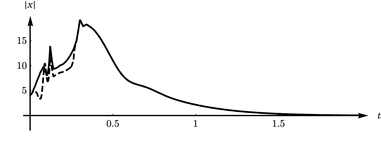
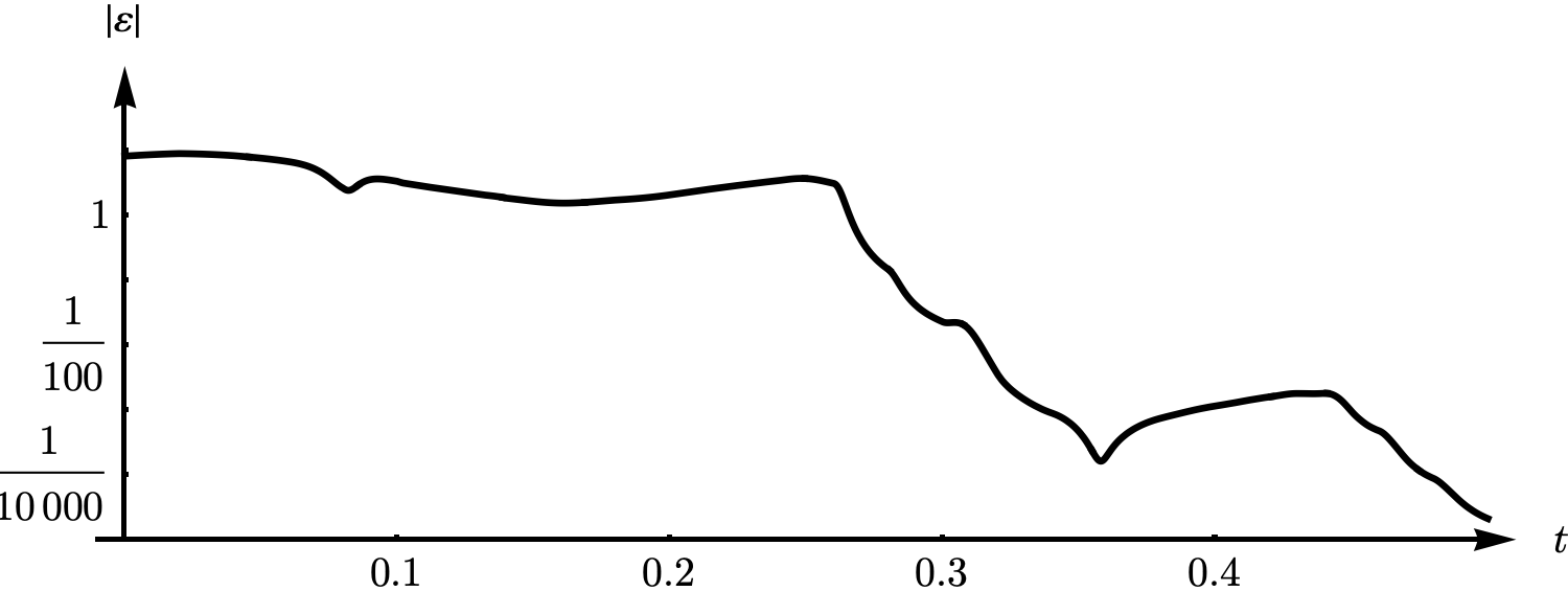
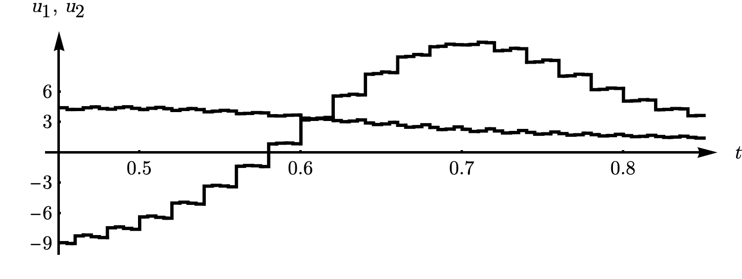
Figure 1: Results of the simulation. The top graph shows the evolution of $|x|$ (plain lines) and $|\hat{x}|$ (dashed lines). The middle one shows the evolution of log error ($\log|\varepsilon|$) of the observer (over the most relevant sub-interval). The bottom graph shows the value of the input $(u_{1},u_{2})$ over a sub-interval as an illustration of the template design.

References

- [1] H. Abou-Kandil, G. Freiling, V. Ionescu, and G. Jank. Matrix Riccati equations. Systems & Control: Foundations & Applications. Birkhäuser Verlag, Basel, 2003. In control and systems theory.
- [2] M. Aguado-Rojas, T. B. Hoàng, W. Pasillas-Lépine, A. Loría, and W. Respondek. A switching observer for a class of nonuniformly observable systems via singular time-rescaling. IEEE Transactions on Automatic Control, 66(12):6071–6076, 2021.
- [3] F. Amato, C. Cosentino, A. S. Fiorillo, and A. Merola. Stabilization of bilinear systems via linear state-feedback control. IEEE Transactions on Circuits and Systems II: Express Briefs, 56(1):76–80, 2009.
- [4] V. Andrieu, L. Brivadis, J.-P. Gauthier, L. Sacchelli, and U. Serres. Exponential stabilizability and observability at the target imply semiglobal exponential stabilizability by templated output feedback. working paper or preprint, Jan. 2024.
- [5] I. Ben Yaacov. The Vandermonde determinant identity in higher dimension. working paper or preprint, May 2017.
- [6] L. Brivadis, J.-P. Gauthier, and L. Sacchelli. Output feedback stabilization of non-uniformly observable systems. Proceedings of the Steklov Institute of Mathematics, 321(1):69–83, 2023.
- [7] L. Brivadis and L. Sacchelli. A switching technique for output feedback stabilization at an unobservable target. In CDC 2021 - 60th IEEE Conference on Decision and Control, pages 3942–3947, Austin, Texas, United States, Dec. 2021.
- [8] L. Brivadis and L. Sacchelli. Output feedback stabilization of non-uniformly observable systems by means of a switched Kalman-like observer. In 22nd World Congress of the International Federation of Automatic Control (IFAC 2023), Yokohama, Japan, July 2023.
- [9] J.-M. Coron. On the stabilization of controllable and observable systems by an output feedback law. Mathematics of Control, Signals and Systems, 7:187–216, 1994.
- [10] R. Goedel, R. G. Sanfelice, and A. R. Teel. Hybrid dynamical systems: modeling stability, and robustness. Princeton, NJ, USA, 2012.
- [11] P. Jouan and J.-P. Gauthier. Finite singularities of nonlinear systems. output stabilization, observability, and observers. Journal of Dynamical and Control systems, 2(2):255–288, 1996.
- [12] C. Kellett, H. Shim, and A. Teel. Robustness of discontinuous feedback via sample and hold control. In Proceedings of the 2002 American Control Conference (IEEE Cat. No.CH37301), volume 5, pages 3512–3517 vol.5, 2002.
- [13] M. Maghenem, W. Pasillas-Lépine, A. Loría, and M. Aguado-Rojas. On observer-based asymptotic stabilization of non-uniformly observable systems via hybrid and smooth control: a case study, 2022.
- [14] D. Nešić and E. Sontag. Input-to-state stabilization of linear systems with positive outputs. Systems & Control Letters, 35(4):245–255, 1998.
- [15] L. Praly and D. Bresch-Pietri. Fonctions de Lyapunov : stabilité. Spartacus-Idh, 2022.
- [16] H. Shim and A. R. Teel. Asymptotic controllability and observability imply semiglobal practical asymptotic stabilizability by sampled-data output feedback. Automatica, 39(3):441–454, 2003.
- [17] H. J. Sussmann. Single-input observability of continuous-time systems. Math. Systems Theory, 12(4):371–393, 1979.
- [18] A. Teel and L. Praly. Global stabilizability and observability imply semi-global stabilizability by output feedback. Systems & Control Letters, 22(5):313–325, 1994.