Improving generalisation via anchor multivariate analysis

Abstract

We introduce a causal regularisation extension to anchor regression (AR) for improved out-of-distribution (OOD) generalisation. We present anchor-compatible losses, aligning with the anchor framework to ensure robustness against distribution shifts. Various multivariate analysis (MVA) algorithms, such as (Orthonormalized) PLS, RRR, and MLR, fall within the anchor framework. We observe that simple regularisation enhances robustness in OOD settings. Estimators for selected algorithms are provided, showcasing consistency and efficacy in synthetic and real-world climate science problems. The empirical validation highlights the versatility of anchor regularisation, emphasizing its compatibility with MVA approaches and its role in enhancing replicability while guarding against distribution shifts. The extended AR framework advances causal inference methodologies, addressing the need for reliable OOD generalisation.

Keywords Distribution shift  $\cdot$ Robust estimation  $\cdot$ Domain generalisation  $\cdot$ Causality  $\cdot$ Multivariate analysis  $\cdot$ Detection and attribution  $\cdot$ Climate Change

1 Introduction

Data sources in contemporary machine learning applications are often heterogeneous, leading to potential distribution shifts Sugiyama and Kawanabe (2012); Shen et al. (2021). This is a particularly relevant problem in computer vision Csurka (2017), healthcare Zhang et al. (2021), finance, Earth and climate sciences (Tuia et al., 2016; Kellenberger et al., 2021) and social sciences, as variations in data patterns can significantly impact model performance and generalisation in the out-of-distribution (OOD) setting, also referred to as domain generalisation (Shen et al., 2021; Zhou et al., 2023). Various frameworks have been proposed to formally address the emergence of distribution shifts during the testing phase Peters et al. (2016); Arjovsky et al. (2020). In cases where the data distribution is entailed by a Structural Causal Model (SCM) Peters et al. (2017), one can consider distribution shifts arising from intervention on specific variables of the SCM. Notably, the Instrumental Variable (IV) regression exhibits robustness to arbitrarily strong interventions (Bowden and Turkington, 1990).

However, pursuing algorithms robust to strong interventions may be overly conservative, especially when prior knowledge is available regarding the intervention strength that generates the distribution shift. Anchor Regression (AR) addresses this challenge by explicitly considering interventions on exogenous variables up to a specified strength (Rothenhäusler et al., 2018). This approach results in a straightforward and manageable regularisation of the classical Ordinary Least Squares (OLS) method, offering a solution for achieving distributionally robust linear regression.

Several AR extensions have been proposed, demonstrating its versatility in handling different scenarios. Notable examples include (1) Kernel Anchor Regression (Shi and Xu, 2023), which extends AR to nonlinear SCMs by working on Reproducing Kernel Hilbert Spaces; (2) Targeted Anchor Regression Oberst et al. (2021), which exploits prior knowledge of the direction of intervention on the anchor variables; and (3) Proxy Anchor Regression Oberst et al. (2021), which addresses cases where the anchor is unobserved but proxy variables are available. Closer to our work, Kook et al. (2022) introduce a distributional extension of AR, expanding its application beyond the $\ell_{2}$ loss to accommodate censored or discrete targets.

All the literature above focuses on regression problems with a one-dimensional target variable and mainly employs least-squared error as the loss function. This paper extends the anchor framework introduced by Rothenhäusler et al. (2018) and contributes in two distinct ways. We first broaden its applicability to various loss functions, ensuring compatibility and robustness against distribution shifts caused by constrained interventions on the anchor variables. This extension redefines conventional MVA algoritms (Borchani et al., 2015; Arenas-Garcia et al., 2013), within the anchor framework, including algorithms such as Partial Least Squares (PLS), Orthonormalized PLS or Reduced Rank Regression (RRR) and Multilinear Regression (MLR). This signifies that their respective loss functions are anchor-compatible , and applying straightforward regularisation enhances their robustness in testing.

After reviewing the AR framework in §2, we study robustness through AR-based regularisation in §3 (anchor-compatible losses and their role in MVAs) and discuss the key links to causality and invariance (cf. §4). Then, we provide estimators for the selected algorithms and examine their consistency (cf. Section 5), supporting our theoretical findings through an extended set of simulation experiments. Finally, we showcase their efficacy in a challenging real-world climate science problem (cf. §6.2). We conclude in §7. The presented AR framework enhances causal inference methods by improving robust OOD generalisation. The code used in this work can be found at this GitHub repository.

2 Anchor framework

This section delineates the class of linear SCMs relevant to our work (§2.2) and offers insight into why anchor regularisation can be employed to obtain distributionally robust estimators (§2.3) for a more general class than the $\ell_{2}$ loss.

2.1 Notation

Bold capital letters $\mathbf{U}$ represent matrices, bold lowercase letters $\mathbf{u}$ denote vectors, regular lowercase letters $u$ signify scalars, and uppercase letters $U$ represent random variables (potentially multivariate) which for notation sakes we assume centred. Given two random vector $U$ and $V$ we define $UV$ as the row-wise stacking operation $UV=(U^{T},V^{T})^{T}$. The symbol $C_{UV}$ denotes Kronecker products involving random variables, i.e. $C_{UV}=UV\otimes UV$and to simplify the notation we write $C_{U}=U\otimes U$. Since we assume centred random variables $\Sigma_{UV}=\mathbb{E}[C_{UV}]$ and $\Sigma_{U}=\mathbb{E}[C_{U}]$. By a slight abuse of notation, we denote $C_{UV|A}=\mathbb{E}\left[UV|A\right]\otimes\mathbb{E}\left[UV|A\right]$ and $\Sigma_{UV|A}$ its expectation. Again for simplification, we write $\sigma_{U}=\mathbb{E}[C_{U}]$ and $\sigma_{UV}=\mathbb{E}[U\otimes V]$. We denote the identity matrix with $\mathbf{I}$, and its dimension is implied by the context when not explicitly stated. Finally, $\|.\|_{F}$ represents the Froebinius norm.

2.2 The Class of Anchor SCM

Figure 1: DAG studied in this work and induced by the SCM in (1).

In the following, we assume the Directed Acyclic Graph (DAG) in Fig. 1, where $X\in\mathbb{R}^{d}$ denotes the observed covariates, $Y\in\mathbb{R}^{p}$ represents the response (or target) variables, $H\in\mathbb{R}^{r}$ are unobserved variables potentially confounding the causal relation between $X$ and $Y$ and $A\in\mathbb{R}^{q}$ the exogenous (so-called anchor) variables. Following Rothenhäusler et al. (2018), we assume that the distribution of $(X,Y,H)$ is entailed by the following linear SCM $\mathcal{C}$:

$$\begin{pmatrix}X\\ Y\\ H\end{pmatrix}=\mathbf{B}\begin{pmatrix}X\\ Y\\ H\end{pmatrix}+\varepsilon+\mathbf{M}A,$$ (1)

where $\mathbf{B}\in\mathbb{R}^{(d+p+r)\times(d+p+r)}$ and $\mathbf{M}\in\mathbb{R}^{(d+p+r)\times q}$ are unknown constant matrices and $\varepsilon\in\mathbb{R}^{d+p+r}$ is a vector of random noise. We assume that $A$ and $\varepsilon$ are independent and have finite variances, $\varepsilon$ components are independent, and $X$ and $Y$ have zero mean. Now, assuming that $(\mathbf{I}-\mathbf{B})$ is invertible, Eq. (1) can be written as:

$$\begin{pmatrix}X\\ Y\\ H\end{pmatrix}=(\mathbf{I}-\mathbf{B})^{-1}(\varepsilon+\mathbf{M}A).$$ (2)

The existence of $(\mathbf{I}-\mathbf{B})^{-1}$ is satisfied if the linear SCM is acyclic. Since our main interest lies in defining the variance-covariance $\Sigma_{XY}$ of $X$ and $Y$, we use $\mathbf{D}\in\mathbb{R}^{(d+p)\times(d+p+r)}$ to express:

$$\begin{pmatrix}X\\ Y\end{pmatrix}=\mathbf{D}(\varepsilon+\mathbf{M}A),$$ (3)

whose existence is implied by the existence of $(\mathbf{I}-\mathbf{B})$ inverse.

2.3 Anchor-Optimal Space

Let us now build upon (3) to illustrate how distributional robustness can be formulated in a causal context and give some intuition of the extension we propose in this work. Later, we will delve into the crucial role of $\Sigma_{XY}$ and its decomposition with $\varepsilon$ and anchor variables $A$. We focus on creating algorithms utilising $\Sigma_{XY}$. Note that, from (3), we can easily express $\Sigma_{XY}$ as

$$\Sigma_{XY} =\mathbf{D}\Sigma_{\varepsilon}\mathbf{D}^{T}+\mathbf{D}\mathbf{M}\Sigma_{A}\mathbf{M}^{T}\mathbf{D}^{T},$$ (4)

which combines the variance from observed exogenous (anchors) and unobserved exogenous (noise) variables.

Let us consider the triplet $(X,Y,H)\sim\operatorname{\mathbb{P}_{\nu}}$, where $\operatorname{\mathbb{P}_{\nu}}=\mathbb{P}^{do(A:=\nu)}_{\mathcal{C}}$ represents the perturbed distribution resulting from intervention (Peters et al., 2017) on the anchor variable $A$, where the distribution of $\nu$ is assumed to be mean-centred. From (4), the interventional variance-covariance matrix $\Sigma_{XY}^{do(A:=\nu)}$ can be expressed as

$$\Sigma_{XY}^{do(A:=\nu)} =\mathbf{D}\Sigma_{\varepsilon}\mathbf{D}^{T}+\mathbf{D}\mathbf{M}\Sigma_{\nu}\mathbf{M}^{T}\mathbf{D}^{T}.$$ (5)

By imposing the constraint $\Sigma_{\nu}\preceq\gamma\Sigma_{A}$ (the rationale for which will be developed in section §3.1), we can bound the interventional variance-covariance matrix $\Sigma_{XY}^{do(A:=\nu)}$ using the training covariances $\Sigma_{\varepsilon}$ and $\Sigma_{A}$. The anchor regularizer parameter $\gamma\in\mathbb{R}^{+}$, controls the amount of causal regularisation by constraining interventions on $A$. This yields the specific distribution class:

$$C^{\gamma}=\{\operatorname{\mathbb{P}_{\nu}}:\Sigma_{\nu}\preceq\gamma\Sigma_{A}\}.$$ (6)

As demonstrated in Eq. (25) and Eq. (24), both $\Sigma_{\varepsilon}$ and $\Sigma_{A}$ can be expressed in terms of $\Sigma_{XY|A}$ and $\Sigma_{XY}$ of the training distribution, which leads to the following inequality:

$$\Sigma_{XY}^{do(A:=\nu)}\preceq\Sigma_{XY}+(\gamma-1)\Sigma_{XY|A}.$$ (7)

Consequently, the interventional covariance matrix $\Sigma_{XY}^{do(A:=\nu)}$

can be bounded using only training data according to Eq. (7). As we will develop in Section 3.1, all algorithms exploiting $\Sigma_{XY}$ can thus be anchor-regularised, leading to distributionally robust estimators.

An example is the $\ell_{2}$ loss, defined for a one-dimensional response variable as $\mathbb{E}[\mathcal{L}(X,Y;\mathbf{b})]=\mathbb{E}[(Y-\mathbf{b}^{T}X)^{2}]=\Sigma_{Y}-2\mathbf{b}^{T}\sigma_{XY}+\mathbf{b}^{T}\Sigma_{X}\mathbf{b}$, which is evidently linear on $\Sigma_{XY}$. Similarly, the PLS algorithm Abdi (2010) aims to find a pair of projection matrices $\mathbf{W}_{x}\in\mathbb{R}^{d\times u}$ and $\mathbf{W}_{y}\in\mathbb{R}^{p\times v}$ that maximise the covariance between the transformed data $X\mathbf{W}_{x}$ and $Y\mathbf{W}_{y}$, i.e. assuming centered $X$ and $Y$, we aim to maximise $\text{tr}(\mathbf{W}_{x}^{T}\Sigma_{XY}\mathbf{W}_{y})$ while constraining $\mathbf{W}_{x}$ and $\mathbf{W}_{y}$ to be orthogonal. Here $u$ and $v$ represent the dimension of the projected spaces. In this case, as the loss is also linear on matrix $\Sigma_{XY}$, i.e. PLS can be anchor-regularised, cf. §3.1.

An intuitive way of thinking about anchor regularisation is to consider that by perturbing the training data (see Eq. (15)), one obtains a dataset that is close to the worst-case scenario we could observe during testing. These observations leads us to consistently define a class of loss functions and demonstrate their distributional robustness properties over the class of perturbed distributions $C^{\gamma}$ defined in (6).

3 Robustness through anchor regularisation

Given $X\in\mathcal{X}$ and $Y\in\mathcal{Y}$, distributionally robust estimation can be formulated as finding a minimiser of the supremum of the population loss under a certain class of distributions:

$$\operatorname{\text{argmin}}_{\mathbf{\Theta}}\sup_{\mathcal{Q}\in\mathbb{Q}}\mathbb{E}_{(X,Y)\sim\mathcal{Q}}[\mathcal{L}(X,Y;\mathbf{\Theta})],$$ (8)

where $\mathbb{Q}$ is a class of distributions and $\mathcal{L}(X,Y;\mathbf{\Theta})$ is a loss function over $X$ and $Y$ with parameters $\mathbf{\Theta}$. In essence, we aim for our model to perform well even in the worst-case scenario when the distribution of $(X,Y)$ belongs to the class of $\mathbb{Q}$. The choice of the class $\mathbb{Q}$ is particularly important as different definitions lead to various types of robustness.

The class $\mathbb{Q}$, often referred to as the uncertainty set, can be constrained using methods such as $f$-divergence (see, e.g., Namkoong and Duchi, 2016) or the Wasserstein distance (see, e.g., Esfahani and Kuhn, 2015). The challenge of OOD generalisation is also closely related to the field of transfer learning (see, e.g., Zhuang et al., 2021). For an in-depth review of OOD generalisation, we recommend consulting (Shen et al., 2021; Zhou et al., 2023).

Of particular interest for this work, causal inference could be understood as a distributionally robust estimation where the class $\mathbb{Q}$ is the class of all distributions arising from arbitrarily large interventions on the variables of an SCM (see Shen et al., 2021, section 4.1.1).

Besides, Rothenhäusler et al. (2018) proposed to bound the intervention strength on the exogenous variable and relax the assumption that it only affects $Y$ through $X$, considering the linear SCM in Fig. 1. By considering the set of distributions $C^{\gamma}$ defined in (6), they demonstrate that their estimator is optimal in the sense of (8) for the $\ell_{2}$ loss.

3.1 anchor-compatible loss

The distributional robustness properties stemming from intervention on the anchor variables arise from the ability to bound the $\Sigma^{do(A:=\nu)}_{XY}$ using the observational covariance matrix $\Sigma_{XY}$ and $\Sigma_{XY|A}$. Consequently, any loss function expressed as a linear function of $\Sigma_{XY}$ can attain distributional robustness similar to AR using anchor regularisation.

Definition 3.1 (anchor-compatible loss).

We say that a loss function $\mathcal{L}(X,Y;\mathbf{\Theta})$ is anchor-compatible if it can be written as

$$\mathcal{L}(X,Y;\mathbf{\Theta})=f_{\mathbf{\Theta}}(C_{XY}),$$ (9)

where $f_{\mathbf{\Theta}}:\mathbb{R}^{d\times p}\to\mathbb{R}$ is a linear form and $\mathbf{\Theta}$ are the parameters to be learned.

This theorem extends Th. 1 in Rothenhäusler et al. (2018) to the previously defined class of loss functions.

Theorem 3.2.

Let the distribution of $(X,Y,H)$ be entailed by the SCM (1) and $\mathcal{L}(X,Y;\mathbf{\Theta})$ be an anchor-compatible loss function. Then for any set of parameters $\mathbf{\Theta}$, and any causal regulariser $\gamma\in\mathbb{R}^{+}$, we have

$$\begin{split}\sup_{\nu\in C^{\gamma}}&\operatorname{\mathbb{E}_{\nu}}[\mathcal{L}(X,Y;\mathbf{\Theta})]=f_{\mathbf{\Theta}}(\Sigma_{XY})\\ +&(\gamma-1)f_{\mathbf{\Theta}}(\Sigma_{XY|A}),\end{split}$$ (10)

where $C^{\gamma}=\{\operatorname{\mathbb{P}_{\nu}}:\Sigma_{\nu}\preceq\gamma\Sigma_{A}\}$.

Proof can be found in the appendix (3.2).

Let us note that the term $f_{\mathbf{\Theta}}(\Sigma_{XY|A})$ could be understood as a causal regulariser enforcing invariance of the loss w.r.t the anchor variable.

For $\gamma=1$, anchor regularisation aligns with unregularised estimation. The theorem suggests that in the case of distributional shifts observed during testing due to constrained intervention on $A$, the anchor-regularised estimator

$$\mathbf{\Theta}^{\gamma}=\operatorname{\text{argmin}}_{\mathbf{\Theta}}f_{\mathbf{\Theta}}(\Sigma_{XY})+(\gamma-1)f_{\mathbf{\Theta}}(\Sigma_{XY|A})$$ (11)

acts as optimal estimators, as per the definition provided in Eq. (8). We will proceed to demonstrate the practical application of this general result to standard Multivariate Analysis (MVA) algorithms.

3.2 Common Multivariate Analysis Algorithms

Table 1: Characterisation of common MVAs with anchor regularisation (loss, constraints, and anchor-compatibility).

	MLR	OPLS	RRR	PLS	CCA
Loss	$\|Y-\mathbf{W}^{T}X\|_{F}^{2}$	$\|Y-\mathbf{U}\mathbf{V}^{T}X\|_{F}^{2}$	$\|Y-\mathbf{W}X\|_{F}^{2}$	$\text{tr}\left(\mathbf{W}_{x}^{T}X^{T}Y\mathbf{W}_{y}\right)$	$\text{tr}\left(\mathbf{W}_{x}^{T}X^{T}Y\mathbf{W}_{y}\right)$
Const.	-	$\mathbf{U}^{T}\mathbf{U}=\mathbf{I}$	rank($\mathbf{W})=\rho$	$\mathbf{W}_{x}^{T}\mathbf{W}_{x}=\mathbf{W}_{y}^{T}\mathbf{W}_{y}=\mathbf{I}$	$\mathbf{W}_{x}^{T}C_{X}\mathbf{W}_{x}=\mathbf{W}_{y}^{T}C_{Y}\mathbf{W}_{y}=\mathbf{I}$
Comp.	✓	✓	✓	✓	✗

A common and straightforward approach to extend least squares (LS) regression to multivariate settings is treating responses independently in multioutput regression (Borchani et al., 2015). This approach aims to identify the regression coefficients $\mathbf{W}$ such that $\hat{Y}=\mathbf{W}^{T}X$, e.g. by solving the LS problem $\widehat{\mathbf{W}}=\operatorname{\text{argmin}}_{\mathbf{W}}\|Y-\mathbf{W}^{T}X\|^{2}_{F}$. When the columns of $Y$ exhibit correlation, RRR addresses a similar optimisation problem assuming that the rank of $\mathbf{W}$ is lower than $\min(d,p)$, see Izenman (1975). Alternatively, in OPLS Arenas-García and Gómez-Verdejo (2015), we do not assume that $\mathbf{W}$ is low rank. Instead, $\mathbf{W}$ is determined by imposing the constraints $\mathbf{W}=\mathbf{V}^{T}\mathbf{U}$, where both $\mathbf{U}$ and $\mathbf{V}$ have a rank $\rho\leq\min(d,p)$.

Additionally, OPLS is commonly solved through matrix deflation, eigenvalue, or generalised eigenvalue decomposition Arenas-García and Gómez-Verdejo (2015). An advantageous property of OPLS is that the columns of the solution $\mathbf{V}$ are ordered based on their predictive performance on $Y$. This is valuable when predicting $Y$ is not the sole objective, and there is interest in learning a relevant information-retaining subspace of $X$ (here $\mathbf{V}^{T}X$). These are natural extensions of LS regression and are anchor-compatible. Please refer to Appendix 8 for further details and proofs.

PLS and CCA are typically preferred when prioritizing learning a pertinent subspace of $X$ over predictive performance. These algoritms aim to maximise the similarity between the latent representations of predictor and target variables. Specifically, PLS assumes the following latent representation:

$$X =\mathbf{P}^{T}T+N_{x},$$

$$Y =\mathbf{Q}^{T}U+N_{y},$$

and seeks to maximise the covariance between $\mathbf{W}_{x}^{T}X$ and $\mathbf{W}_{y}^{T}Y$, while CCA aims to maximise the correlation between the estimated latent spaces. Correlation as a similarity measure ensures equal importance for each dimension in the learned latent space, independent of data variance.

PLS, being anchor (see Proposition 8.2), benefits from causal regularisation for distributional robustness. In contrast, CCA lacks anchor compatibility due to nonlinearity in its loss function concerning variance-covariance (see §8.3). As illustrated in Fig. 2, CCA shows reduced robustness under interventions on the anchor variable’s variance. Recognizing the established equivalence between CCA and OPLS (Sun et al., 2009), it may appear puzzling that one algorithm is anchor-compatible while the other is not. We delve deeper into this matter in the supplementary (§8).

4 Towards causality, invariance and stability

Given the well-established connection between causality and invariant predictions (see, for instance Bühlmann (2020) Prop. 3.1), exploring the relationship between anchor regularisation, causality, and invariance could offer valuable insights.

For instance, IV regression assumes that the noise term $\varepsilon_{y}$ is independent of the instrument (or anchor) variable $A$ (i.e., $\varepsilon_{y}\perp\!\!\!\perp A)$ thus IV estimations can be performed using the moment restriction Newey and Powell (2003) $\mathbb{E}[Y-b^{T}X|A]=0$, which can be related to the right term of Eq. (10) for anchor-regularised $\ell_{2}$ loss. Thus, as $\gamma\to\infty$, the anchor-regularised loss converges to the IV estimation, i.e.

$$\mathbf{\Theta}^{IV} =\operatorname{\text{argmin}}_{\mathbf{\Theta}}f_{\mathbf{\Theta}}(\Sigma_{XY|A})=\lim_{\gamma\to+\infty}\mathbf{\Theta}^{\gamma}.$$ (12)

Increasing $\gamma$ ensures stable predictive performance by promoting robustness to shifts in the distribution of $X$ resulting from interventions on the anchor.

Another notable scenario is the partialling-out (PA) setting, closely related to double machine learning (see e.g. Chernozhukov et al., 2017), where the anchor variables directly influence both $X$ and $Y$, and there is no hidden confounder $H$.

In this setup, the causal effect is estimated by deriving residuals of $X$ and $Y$ predicted by $A$, followed by estimating the regression coefficient of the residuals of $X$ on the residuals of $Y$. This process is equivalent to estimating the causal effect of $X$ on $Y$ within the orthogonal complement space of $A$. Thus, an anchor-regularised algorithm with $\gamma=0$ is akin to PA estimation.

$$\mathbf{\Theta}^{PA} =\operatorname{\text{argmin}}_{\mathbf{\Theta}}f_{\mathbf{\Theta}}(\Sigma_{XY|A^{\perp}})=\lim_{\gamma\to 0}\mathbf{\Theta}^{\gamma},$$ (13)

where $A^{\perp}=\mathbf{I}-A$ is the orthogonal complement of $A$. Hence, PA solves the minimax problem Eq. (10) for an empty set Eq. (6) and is thus optimal under distribution shift arising from null intervention on $A$. Note that, in some instances, the parameters $\mathbf{\Theta}^{\gamma}$ remain consistent across all $\gamma\in[0,\infty]$, resulting in what we term as anchor stability. Under these circumstances, and subject to relatively mild assumptions outlined in Rothenhäusler et al. (2018) section 3.2, the parameters $\mathbf{\Theta}$ can be causally interpreted, as demonstrated in (Rothenhäusler et al., 2018, Th. 4), indicating the absence of a confounder $H$ between $X$ and $Y$.

5 Estimators

In the previous sections, we derived properties of various MVA methods in the population case. We consider now the sample setting where we are given $n$ i.i.d observations of $(X,Y,A)$. As customary, observations are collectively organised row-wise, in the following matrices, $\mathbf{X}\in\mathbb{R}^{n\times d}$, $\mathbf{Y}\in\mathbb{R}^{n\times p}$ and $\mathbf{A}\in\mathbb{R}^{n\times q}$. For a given anchor-compatible loss $\mathcal{L}(X,Y;\mathbf{\Theta})=f_{\mathbf{\Theta}}(C_{XY})$, we propose to consider a simple estimator of the population parameter $\mathbf{\Theta}^{\gamma}$, obtained by the plug-in principle:

$$\widehat{\mathbf{\Theta}}^{\gamma}=\operatorname{\text{argmin}}_{\mathbf{\Theta}}f_{\mathbf{\Theta}}(\mathbf{S}_{XY})+(\gamma-1)f_{\mathbf{\Theta}}(\mathbf{S}_{XY|A}),$$ (14)

where $\mathbf{S}_{XY}$ and $\mathbf{S}_{XY|A}$ are respectively the empirical estimators of $\Sigma_{XY}$ and of $\Sigma_{XY|A}$.

As proved by Rothenhäusler et al. (2018), $\widehat{\mathbf{\Theta}}^{\gamma}$ can be computed by transforming the training data:

$$\begin{split}\tilde{\mathbf{X}}&=(\mathbf{I}+(\sqrt{\gamma}-1)\Pi_{\mathbf{A}})\mathbf{X},\\ \tilde{\mathbf{Y}}&=(\mathbf{I}+(\sqrt{\gamma}-1)\Pi_{\mathbf{A}})\mathbf{Y},\end{split}$$ (15)

where $\Pi_{\mathbf{A}}=\mathbf{A}(\mathbf{A}^{T}\mathbf{A})^{-1}\mathbf{A}^{T}\in\mathbb{R}^{n\times n}$ projects onto the column space of $\mathbf{A}$, assuming that $\mathbf{A}^{T}\mathbf{A}$ is invertible and $\mathbf{X}$ and $\mathbf{Y}$ are centered.

Finally, build the estimator $\widehat{\mathbf{\Theta}}^{\gamma}=\operatorname{\text{argmin}}_{\mathbf{\Theta}}f_{\mathbf{\Theta}}(\mathbf{S}_{\tilde{X}\tilde{Y}})$, where $\mathbf{S}_{\tilde{X}\tilde{Y}}$ is the empirical variance-covariance of the projected data defined in Eq.  (15).

Consistency

From the law of large numbers, the empirical covariance matrix of $(X,Y,A)$ converges to its empirical covariance matrix, i.e., $\mathbf{S}_{XY}\xrightarrow[n\to\infty]{}\Sigma_{XY}$. Thus, the consistency of the anchor-regularised estimator depends on the consistency of the original estimator. For continuous functions $f$, we have by continuity that $\mathbf{\widehat{\Theta}}^{\gamma}\xrightarrow[n\to\infty]{}\mathbf{\Theta}^{\gamma}$ (see Rothenhäusler et al., 2018, section 4.1).

Computational Complexity

The computational cost of projecting $X$ and $Y$ into the span of $A$ involves computing the covariance matrix of $A$ (of cost $O(nr^{2})$), inverting it (of cost $O(r^{3})$), and two matrix products (of cost $O(nrp)$ and $O(nr^{2})$), resulting in a total complexity of $O(nr^{2}+nrp+r^{3})$. Assuming the unregularised MVA algorithm’s computational cost is $c$, the complexity of its anchor-regularised version is $O(c+nr^{2}+nrp+r^{3})$.

Parameter selection

When knowledge about the graph and anchor variable distributional shift is available, one can estimate the optimal $\gamma$ for robustness against worst-case scenarios. For instance, if the expected anchor variable perturbation strength is up to $1.5$, Rothenhäusler et al. (2018) recommends $\gamma=1.5$. Refer to Section 8.2 of Rothenhäusler et al. (2018) for a detailed estimation approach. Without prior knowledge, various strategies can be considered: Rothenhäusler et al. (2018) propose $\gamma=2$ as a suitable default choice, while Sippel et al. (2021) and Székely et al. (2022) suggest selecting $\gamma$ as a trade-off between prediction error (MSE or $R^{2}$ score) and the correlation between residuals and the anchor variable, or the value of projected residuals in the anchor variable’s span. Similar strategies have been proposed in deemed related algorithms Cortés-Andrés et al. (2022); Li et al. (2022).

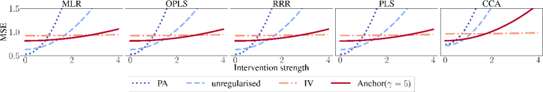
Figure 2: Robustness to increasing perturbation strength for PA, unregularised, IV, anchor-regularised ($\gamma=5$) algorithms ( MLR, OPLS, RRR, PLS and CCA). Anchor versions show robustness in terms of $R^{2}$ for bounded intervention strength.

High Dimensional Estimators

Dealing with high dimensional data challenges estimators and often requires introducing regularisation Bühlmann and Van De Geer (2011); Candes and Tao (2007). Regularisation has been generally introduced to control models’ capacity and avoid overfitting Girosi et al. (1995); Tibshirani (1996); Hastie et al. (2009), but also to introduce prior (domain) knowledge in the algorithms, as in AR. Adding a regularisation term $\Omega(\|\mathbf{\Theta}\|)$ to the empirical loss in Eq. (14) leads to estimate $\mathbf{\Theta}$ as

$$\begin{split}\widehat{\mathbf{\Theta}}^{\gamma}=\operatorname{\text{argmin}}_{\mathbf{\Theta}}f_{\mathbf{\Theta}}&(\mathbf{S}_{XY})\\ +(\gamma-1)&f_{\mathbf{\Theta}}(\mathbf{S}_{XY|A})+\Omega(\|\mathbf{\Theta}\|).\end{split}$$ (16)

In CCA, OPLS, and PLS regression (or the rank in RRR), the number of components can be viewed as regularisation hyperparameters. Consequently, the optimisation task for anchor-regularised MVA algorithms may involve many hyperparameters. For instance, in anchor-regularised Reduced Rank Ridge Regression (A-RRRR), three hyperparameters require tuning: $\ell_{2}$ regularisation $\alpha$, rank $\rho$, and anchor regularisation $\gamma$. Since each hyperparameter optimization addresses different objectives, it may be impractical to optimise all of them simultaneously. Sippel et al. (2021) advise selecting hyperparameters as a trade-off between prediction performance (e.g., MSE or $R^{2}$) and a proxy of robustness to anchor intervention (e.g. correlation between anchor and residuals).

6 Experiments

Our theoretical findings are substantiated through an extensive series of experiments that highlight the robustness of anchor-regularised MVA algorithms to increasing perturbation strength (cf. Section 6.1). Furthermore, we provide a concrete high-dimensional example to elucidate the process of hyperparameter selection (cf. Section 6.1), and demonstrate its practical relevance by showcasing how anchor regularisation enhances climate predictions in a real-world Climate Science application (cf. Section 6.2).

6.1 Simulation Experiments

Robustness to Perturbation Strength

To demonstrate how anchor regularisation can be applied with different multivariate analysis algorithms, we adapt the experiments from (Rothenhäusler et al., 2018, Sec. 2.2) to a multioutput setting.

We assume that the training data $(A,X,Y)$ follows a distribution based on the linear SCM:

$$\begin{split}\varepsilon_{A},\varepsilon_{H},&\varepsilon_{X},\varepsilon_{Y}\sim\mathcal{N}(0,1)\\ A&\leftarrow\varepsilon_{A}\\ H&\leftarrow\varepsilon_{H}\\ X&\leftarrow A+H+\varepsilon_{X}\\ Y&\leftarrow\mathbf{W}^{T}X+H+\varepsilon_{Y},\end{split}$$ (17)

where $X$ and $Y$ are multivariate, of respective dimension $d=p=10$ ($d=p=300$ with $n=200$ in the high dimensional setting), and $\mathbf{C}$ is low rank (see Supplementary  10.1 for more details on the experiments settings). We generate test data by intervening on the anchor variable’s distribution, setting $A\sim\mathcal{N}(0,t)$, where $t$ is the perturbation strength. Each MVA algorithm assumes oracle knowledge of the rank $\rho$ of $\mathbf{C}$, aligning RRR’s rank, PLS regression’s component count, and CCA accordingly. IV setting ($A$ only affects $Y$ through $X$) and we show that even in this scenario, anchor regularised algorithms (with $\gamma=5$) outperform the PA, IV, and unregularised algorithms.

Shown in Fig. 2, all anchor-compatible algorithms exhibit robustness to distribution shifts. Anchor-regularised models (with $\gamma=5$) excel with bounded-strength interventions; PA regularisation is optimal for weak interventions; and IV regularisation for unlimited perturbation strength. Overall, anchor-regularised algorithms maintain stable performance across various perturbation strengths.

We also conducted a set of high-dimensional experiments ($p\gg n$ and $d\gg n$) using RRR and MLR both regularised with $\ell_{2}$ norm (ridge regularisation). In both cases, the anchor-regularised algorithms exhibit robustness to increasing perturbation strength (see Fig. 6 in §10.1). This is also the case when $A$ is a confounder (affecting both $X$ and $Y$, potentially through $H$), in which case anchor-regularised algorithms present are equally optimal for a wide range of perturbation strength (see Fig. 8 in §10.1). Though not as pronounced as in anchor-compatible algorithms, anchor-regularised CCA also displays robustness to perturbations in $A$, prompting further investigation into its behaviour.

Hyperparameter Selection

We showcase how hyperparameter selection can be performed through a simulation experiment in a high-dimensional setting using an anchor-regularised version of Reduced Rank Ridge Regression (Mukherjee and Zhu, 2011).

In this setting, we are given three hyperparameters: $\gamma$ enforces robustness to intervention on the anchor, $\alpha$ and $\rho$ aim to maximise prediction performance. Following (Sippel et al., 2021) we select hyperparameters as a trade-off between predictive performance (measured via MSE) and correlation between anchor and residuals. We give equal weights to both objectives but this can be adapted regarding the knowledge available and the application. Thus hyperparameters are selected at testing such that they minimise the combination of the two objectives. Fig. 3 shows how augmenting regularisation for distributional robustness to anchor intervention often reduces predictive performance in the training sample (Fig. 3.A), yet the trade-off translates into improved predictive performance in testing samples. More details about this experiment setting are in  §10.2.

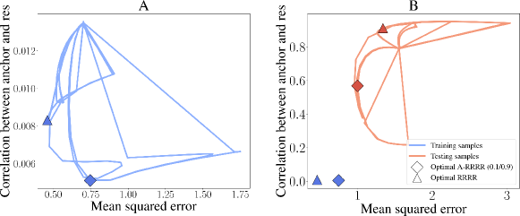
Figure 3: Pareto front for hyperparameters $(\gamma,\alpha,\rho)$ in RRRR and A-RRRR. For each pair $(\gamma,\alpha)$, $\rho$ is selected to minimise the weighted sum of objectives (equal weights given here).

6.2 Real Experiment: Robust Climate Prediction

We showcase the efficacy of our approach in a real-world application within the Detection and Attribution of Climate Change (D&A) domain. We extend the methodology of Sippel et al. (2021), who utilised AR for robust detection of forced warming against increased climate variability, by applying it to predict multidimensional local climate responses. Given the increased variability observed in recent climate models Parsons et al. (2020) and observations (DelSole, 2006; Kociuba and Power, 2015; Cheung et al., 2017), our approach aims to ensure robustness against potential underestimation of decadal and multidecadal internal climate variability (Parsons et al., 2020; Mcgregor et al., 2018).

Objective

Specifically, our objective is to use a $p$-dimensional temperature field $X_{\text{mod}}$ to predict a temperature response $Y_{\text{mod}}^{\text{forced}}\in\mathbb{R}^{p}$ to external forcings (such as greenhouse gas emissions, aerosols, solar radiation, or volcanic activity), a crucial step in detecting warming using the fingerprint method (see Hegerl et al., 1996), while ensuring robustness to climate’s Decadal Internal Variability (DIV). To achieve this, we follow Sippel et al. (2021), leveraging multiple climate models from the Climate Model Intercomparison Project (CMIP), both Phase 5 Taylor et al. (2011) and 6 Eyring et al. (2016) (CMIP5 and CMIP6). Specifically, we employ four models (CCSM4, NorCPM1, CESM2, HadCM3) characterised by lower-scale DIV to train our MVA algorithm and validate its robustness using anchor regularisation against models exhibiting higher-scale DIV (CNRM-CM6-1, CNRM-ESM2-1, IPSL-CM6A-LR).

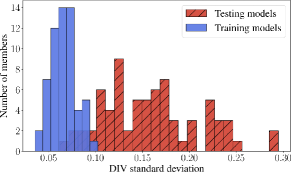
Figure 4: Standard deviation of DIV among training (red) and testing (blue) model members.

Estimators

As a multivariate algorithm, we employ RRRR since both the predictors (temperature fields) and the target (temperature response to external forcing) variables exhibit correlation structures due to spatial autocorrelation. Since both $\alpha$ and $\rho$ in RRRR serve to regularise the regression, we optimise them using cross-validation across the training models. We consider two levels of anchor regularisation: $\gamma=5$ (low regularisation) and $\gamma=100$ to induce high robustness to a potential increase in DIV. We evaluate our results regarding two metrics: $R^{2}$ score (a standard metric when predicting spatial fields) and mean correlation between the anchor (DIV) and the regression residuals (Sippel et al., 2021; Székely et al., 2022).

Data

We selected seven models from the CMIP5 and CMIP6 archives, each containing at least $8$ members from historical simulations, to ensure accurate estimation of the climate response (refer to Tab. 2 for detailed model information). The data preprocessing procedure for each model involves re-gridding surface air temperature data to a regular $5\mathrm{°}$$\times$$5\mathrm{°}$ grid and computing yearly anomalies by subtracting the mean surface air temperature for the reference period: years $1850-1900$. The forced response $Y^{\text{forced}}_{\text{mod}}$ is obtained using a standard approach (see Deser et al., 2020, and Supplementary details), averaging over all available members in each model. Furthermore, we use DIV as a proxy for multidecadal climate internal variability (see Parsons et al., 2020), achieved by removing the global forced response to global temperature and smoothing it using a $10$-year running mean. This procedure is commonly employed for estimating the multidecadal variability of the climate system (see Sippel et al., 2021; Deser et al., 2020, for further details). Finally, all data are standardised.

Evaluation procedure

We categorise the models into two groups (low and high variability) based on the distribution of the standard deviation of their DIV among the members of each model. As depicted in Fig. 4, a significant proportion of members used for training display a notably smaller magnitude of DIV. Hyperparameters $(\alpha,\rho)$ are selected through a leave-half-models-out cross-validation procedure. Given $k=4$ training models, we randomly select $k/2$ models for training and $k/2$ models for validation, and repeated $B=10$ times. We use $500$ samples from each model to ensure equal weights are given to each training model in the learning algorithm, despite variations in the number of members. For each of the $B$ train/validation splits, we train an RRRR model and select the hyperparameters that yield the highest averaged $R^{2}$ score across the $B$ sampling splits. $R^{2}$ provides a performance measure comparable across regions and is typically used when predicting spatial variables (see e.g. Sippel et al., 2019). Hyperparameter $\alpha$ is selected from $20$ candidates in a logarithmically-spaced sequence ($\lambda\in[1;10^{6}]$), and $\rho$ is selected from $21$ candidates in a linearly-spaced integer sequence ($\rho\in[300;600]$).

Results

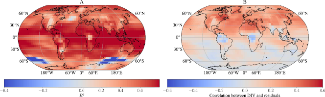
Figure 14: A-RRRR ($\gamma=100$) scores. (A) $R^{2}$ scores. (B) Correlation between DIV and residuals.

For both anchor-regularised RRRR (A-RRRR) with $\gamma=5$ and $\gamma=100$, we observe an improvement in both metrics in the testing set (respectively $0.537$ and $0.533$ of $R^{2}$ for A-RRRR and $0.506$ for unregularised RRRR), while experiencing a slight decrease of performance in the training samples ($0.510$ of $R^{2}$ for unregularised RRRR and respectively $0.500$ and $0.487$ for both A-RRRR). As the latter strongly protects against shifts in DIV, we notice that its mean correlation between residuals and DIV is lower, albeit with a slight decrease in the $R^{2}$ score (see Table 3 in §11). Spatially, we observe (Fig. 5) that anchor-regularised RRRR performs better in the northern hemisphere, particularly in regions where the residuals are highly correlated with DIV and in the northern hemisphere where unregularised RRRR performs poorly (see Figs. 14 and 15 in §11).

Conversely, we observe a decrease in the performance of A-RRRR in regions where unregularised RRRR already performs well or where residuals are anti-correlated with DIV. The latter challenge might be addressed by considering regional proxies of internal variability instead of a global one, which does not always accurately represent local internal variability.

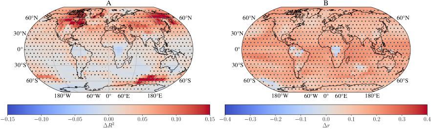
Figure 5: (A) $R^{2}$ score differences between A-RRRR (for $\gamma=5$) and RRRR for testing models. Red values imply that anchor regularisation gives better estimates (larger $R^{2}$ score). (B) Differences of correlation between residuals and DIV ($r$) between anchor-regularised RRRR (for $\gamma=5$) and RRRR for testing models. Red values imply that anchor regularisation gives a lower correlation between residuals and DIV. Regions where A-RRRR perform better are hatched with dots.

These results suggest the potential of using anchor-regularised multi-output algorithms in D&A studies to detect and attribute local responses to external forcings, a fundamental problem in climate science.

7 Conclusion

In this study, we extend the causal framework of anchor regression proposed by Rothenhäusler et al. (2018), demonstrating the versatility of their regularisation approach across a wide range of MVA algorithms. Given the significant challenge of generalising models to OOD data in machine learning, we advocate for integrating anchor regularisation into a broader class of MVA algorithms, including RRR, OPLS, or PLS regression, particularly when prior knowledge is available about the reasons for distribution shifts. Moreover, we highlight that anchor regularisation offers an interesting trade-off between prediction performance and invariance to distribution shifts, addressing concerns regarding over-conservativeness in some cases. Additionally, our application of anchor regularisation in real-world scenarios underscores its practical utility. Future theoretical advancements will entail extending the formulation nonlinear cases using kernel methods Po-Chedley et al. (2022). Furthermore, an intriguing avenue for exploration is understanding how statistical learning algorithms incompatible with anchor regularisation behave when this regularisation is applied. On the application front, we aim to investigate how anchor regularisation, in conjunction with various MVA algorithms, can be leveraged to detect forced responses to more complex climate variables (e.g., precipitation or temperature and their extremes) and attribute them to external forcing sources such as greenhouse gas or aerosol emissions (anthropogenic) or natural phenomena like solar radiation and volcanic activity. We anticipate a broad development and application of the presented and future anchor-regularised methods across various fields of science.

Impact statement

This paper contributes to Machine Learning by showcasing the application of anchor regularisation in both general tasks in multivariate data analysis and statistics and in the specific context of Detection and Attribution (D&A) studies in climate science. The broader impact of this work lies in its potential to enhance the robustness and reliability of algorithms across various domains, including those with societal, economic and environmental implications. Specifically, in climate science, where accurate detection and attribution of climate change impacts are crucial for informed decision-making, our findings demonstrate how anchor regularisation can improve the reliability of predictive models. By addressing distributional shifts and enhancing model robustness, our approach can potentially strengthen the scientific basis for policy-making and adaptation strategies while contributing to the broader understanding and mitigation of climate change impacts.

8 Robustness of common multivariate analysis algorithm

In this section, we aim to prove the compatibility and incompatibility of some standard multivariate analysis algorithms. We assume that the $(X,Y,H,A)$ distribution be entailed in Eq. (1).

A natural extension of Ordinary Least Squares ($\ell_{2}$) regression to the multioutput case is to solve an OLS problem for each output, which is equivalent to solving the optimisation problem:

$$\min_{\mathbf{W}\in\mathbb{R}^{d\times p}}\mathbb{E}\|Y-\mathbf{W}^{T}X\|_{F}^{2},$$ (18)

also known as multilinear (or multioutput) regression. Extra constraints on the regression coefficients can be added, leading, for example, to Reduced Rank Regression by constraining $\mathbf{W}$ to be of rank $\rho<\min(p,d)$. This constraint resembles constraining $\mathbf{W}$ to have the form $\mathbf{V}^{T}\mathbf{U}$, with $\mathbf{U}\in\mathbb{R}^{\rho\times d}$ and $\mathbf{V}\in\mathbb{R}^{\rho\times p}$.

This formulation is closely related to the formulation of Orthogonalised Partial Least Squares with an extra constraint on the ordering of the columns of $\mathbf{V}^{T}X$ based on their predictive performance on $Y$. Therefore, we derive the proof of anchor compatibility for the multilinear regression setting, which directly extends to anchor compatibility of OPLS and Reduced Rank Regression.

Since both OPLS and RRR aim to achieve the same objective as defined in Eq. (19) with different constraints on regression coefficients $\mathbf{W}$, we prove the general anchor compatibility of MLR, but this extends to OPLS and RRR.

Proposition 8.1 (Multilinear, Reduced Rank and Orthonormalised Partial Least Square Regression are anchor-compatible.).

The algorithm minimising the expectation of the following loss function:

$$\mathcal{L}(X,Y;\mathbf{\Theta})=\|Y-\mathbf{W}^{T}X\|^{2}_{F}$$ (19)

is anchor-compatible. Here $\|.\|_{F}$ defines the Froebinius norm.

Proof.

The proof of this proposition is straightforward, observing that the loss can be written as:

$$\mathcal{L}(X,Y;\mathbf{\Theta})=\sigma_{Y}-\mathbf{W}^{T}\sigma_{XY}+\mathbf{W}^{T}\sigma_{X}\mathbf{W},$$ (20)

which is linear over the variance-covariance $\Sigma_{XY}$.

∎

Another type of Multivariate Analysis algorithm is not aimed at minimising prediction error. Instead, it focuses on maximising the similarity between latent representations of the predictors $X\mathbf{W}_{x}$ and the target $Y\mathbf{W}_{y}$. A standard measure of this similarity is covariance, leading directly to the Partial Least Squares (PLS) algorithm, for which we now present anchor compatibility.

Proposition 8.2 (Partial Least Square regression is anchor-compatible.).

The PLS Regression algorithm maximising the expectation of the following loss function is anchor-compatible:

$$\mathcal{L}(X,Y;\mathbf{W})=\frac{\text{tr}(\mathbf{W_{x}}^{T}C_{XY}\mathbf{W}_{y})}{\sqrt{\text{tr}(\mathbf{W_{x}}^{T}\mathbf{W_{x}})}\sqrt{\text{tr}(\mathbf{W_{y}}^{T}\mathbf{W_{y}})}}.$$ (21)

Proof.

The loss function Eq. 21 is clearly linear with respect to the variance-covariance $\Sigma_{XY}$, which is sufficient to ensure the anchor compatibility of PLS regression. ∎

On the other hand, one could consider correlation as a measure of the similarity between the learned latent spaces, aiming to account for potential differences in the variance of each variable and thus assigning equal weight to each dimension of the latent space. This approach is generally known as Canonical Correlation Analysis (CCA) or PLS mode B. By considering the variance of the latent representation of the predictors and the target, we sacrifice linearity with respect to the variance-covariance of $X$ and $Y$ (as illustrated in Eq. 22), making CCA incompatible with anchor regularisation.

Example 8.3 (Canonical Correlation Analysis is not anchor-compatible.).

The Canonical Correlation Analysis solving the optimisation problem

$$\mathcal{L}(X;\mathbf{W})=\frac{\text{tr}(\mathbf{W_{x}}^{T}\Sigma_{XY}\mathbf{W_{y}})}{\sqrt{\text{tr}(\mathbf{W_{x}}^{T}\Sigma_{X}\mathbf{W_{x}})}\sqrt{\text{tr}(\mathbf{W_{y}}^{T}\Sigma_{Y}\mathbf{W_{y}})}}$$ (22)

is not anchor-compatible as it is not linear over the variance-covariance matrix. This explains the different behaviour taken by anchor regularisation in Fig. 2 by the anchor-regularised CCA.

This is illustrated in Fig. 2, where we can observe that anchor-regularised CCA exhibits a distinct behavior compared to anchor-compatible MVA algorithms. It would be of interest to investigate to which extent the incompatibility of CCA with anchor regularisation impacts its distributional robustness properties and if its anchor regularisation could still be of interest.

OPLS formulations and their relation to CCA

There are two versions of OPLS: the standard eigenvalue decomposition (EVD) and the generalized eigenvalue (GEV) formulations Arenas-García and Gómez-Verdejo [2015]. In our work, we implement EVD-OPLS whose optimization problem is

$$\min_{\mathbf{U},\mathbf{V}} \|Y-\mathbf{U}\mathbf{V}^{T}X\|_{F}^{2}$$

$$\text{s.t. }\ \mathbf{U}^{T}\mathbf{U}=\mathbf{I}.$$

EVD-OPLS is linear in $C_{XY}$ and is, therefore, an anchor-compatible loss. On the other hand, the GEV-OPLS loss is

$$\min_{\mathbf{U},\mathbf{V}} \|Y-\mathbf{U}\mathbf{V}^{T}X\|_{F}^{2}$$

$$\text{s.t. }\ \mathbf{V}^{T}C_{X}\mathbf{V}=\mathbf{I}$$

Viewing the optimization for $\mathbf{V}$ as a generalized eigenvalue decomposition problem by absorbing the constraint into the loss gives us the equivalent optimization

$$\min_{\mathbf{v}}\frac{\mathbf{v}^{T}X^{T}YY^{T}X\mathbf{v}}{\mathbf{v}^{T}C_{X}\mathbf{v}}.$$

This is clearly not linear in $C_{XY}$ because it is not linear in $C_{X}=X^{T}X$.

Furthermore, GEV-OPLS and CCA are shown to be equivalent up to an orthogonal rotation [see Sun et al., 2009, Theorem 2], and by similar reasoning, CCA is also not anchor-compatible.

9 Proofs

9.1 Proof of Theorem 3.2

Proof.

Let’s first note that from the SCM Eq.  1 we have the following decomposition:

$$f(C_{XY}) =f(\mathbf{D}C_{\varepsilon}\mathbf{D}^{T}+\mathbf{D}\mathbf{M}C_{A}\mathbf{M}^{T}\mathbf{D}^{T})$$

$$=f(\mathbf{D}C_{\varepsilon}\mathbf{D}^{T})+f(\mathbf{D}\mathbf{M}C_{A}\mathbf{M}^{T}\mathbf{D}^{T})$$

by linearity of $f$. Thus when taking the supremum of the expectation of $f(C_{XY})$ over $C^{\gamma}$, we get

$$\sup_{\nu\in C^{\gamma}}\operatorname{\mathbb{E}_{\nu}}[f(C_{XY})] =f(\mathbf{D}\Sigma_{\varepsilon}\mathbf{D}^{T})$$

$$+\sup_{\nu\in C^{\gamma}}f(\mathbf{D}\mathbf{M}\Sigma_{\nu}\mathbf{M}^{T}\mathbf{D}^{T}),$$

since $f(\mathbf{D}\Sigma_{\varepsilon}\mathbf{D}^{T})$ is not affected by the intervention. Using the definition of $C^{\gamma}$ leads to

$$\begin{split}\sup_{\nu\in C^{\gamma}}\operatorname{\mathbb{E}_{\nu}}[f(C_{XY})]&=f(\mathbf{D}\Sigma_{\varepsilon}\mathbf{D}^{T})\\ &+\gamma f(\mathbf{D}\mathbf{M}\Sigma_{A}\mathbf{M}^{T}\mathbf{D}^{T}).\end{split}$$ (23)

Let’s now note that for $(A,X,Y)\sim\mathbb{P}_{\text{train}}$ we have

$$\operatorname{\mathbb{E}_{\text{train}}}\left[\begin{pmatrix}X\\ Y\end{pmatrix}|A\right] =\mathbf{D}\operatorname{\mathbb{E}_{\text{train}}}[\varepsilon|A]+\mathbf{D}\mathbf{M}\operatorname{\mathbb{E}_{\text{train}}}[A|A]$$

$$=\mathbf{D}\mathbf{M}A,$$

where $\mathbb{P}_{\text{train}}$ is the training distribution.

As $\varepsilon$ is mean centred and independent of $A$. Thus, we can write

$$f(C_{XY|A})=f(\mathbf{D}\mathbf{M}C_{A}\mathbf{M}^{T}\mathbf{D}^{T})$$

by linearity of $f$. Taking its expectation over the training distribution, we get

$$\operatorname{\mathbb{E}_{\text{train}}}[f(C_{XY|A})]=f(\mathbf{D}\mathbf{M}\Sigma_{A}\mathbf{M}^{T}\mathbf{D}^{T}),$$ (24)

which is similar to the right term of Eq. (23) as $\operatorname{\mathbb{E}_{\text{train}}}[f(C_{XY|A})]=f(\Sigma_{XY|A})$. A similar reasoning leads to

$$\operatorname{\mathbb{E}_{\text{train}}}[f(C_{XY})]-\operatorname{\mathbb{E}_{\text{train}}}[f(C_{XY|A})] =f(\mathbf{D}\Sigma_{\varepsilon}\mathbf{D}^{T}).$$ (25)

Pluging-in Eq. (24) and Eq. (25) in Eq. (23) we get

$$\sup_{\nu\in C^{\gamma}} \operatorname{\mathbb{E}_{\nu}}[f(C_{XY})]=$$

$$\operatorname{\mathbb{E}_{\text{train}}}[f(C_{XY})]+(\gamma-1)\operatorname{\mathbb{E}_{\text{train}}}[f(C_{XY|A})]$$

$$= f(\Sigma_{XY})+(\gamma-1)f(\Sigma_{XY|A}),$$

which concludes the proof. ∎

9.2 Proof of Equivalence for Transformed Data

Proof.

From

$$\begin{split}\tilde{\mathbf{X}}&=(\mathbf{I}+(\sqrt{\gamma}-1)\Pi_{\mathbf{A}})\mathbf{X}\\ \tilde{\mathbf{Y}}&=(\mathbf{I}+(\sqrt{\gamma}-1)\Pi_{\mathbf{A}})\mathbf{Y},\end{split}$$ (26)

we can easily derive that

$$\mathbf{S}_{\tilde{X}\tilde{Y}}= \frac{1}{n-1}(\tilde{\mathbf{X}}\tilde{\mathbf{Y}})^{T}(\tilde{\mathbf{X}}\tilde{\mathbf{Y}})$$

$$= \frac{1}{n-1}((\mathbf{X}\mathbf{Y}+(\sqrt{\gamma}-1)\Pi_{\mathbf{A}}\mathbf{X}\mathbf{Y})^{T}$$

$$(\mathbf{X}\mathbf{Y}+(\sqrt{\gamma}-1)\Pi_{\mathbf{A}}\mathbf{X}\mathbf{Y}))$$

As $\Pi_{\mathbf{A}}$ is an orthogonal projection, we have that $(\mathbf{X}\mathbf{Y})^{T}(\Pi_{\mathbf{A}}\mathbf{X}\mathbf{Y})=\Pi_{\mathbf{A}}(\mathbf{X}\mathbf{Y})^{T}\mathbf{X}\mathbf{Y}=\mathbf{S}_{XY|A}$, leading to

$$= \mathbf{S}_{XY}+2(\sqrt{\gamma}-1)\mathbf{S}_{XY|A}$$

$$+ (\sqrt{\gamma}-1)^{2}\mathbf{S}_{XY|A}$$

$$= \mathbf{S}_{XY}+(\gamma-1)\mathbf{S}_{XY|A}.$$

Thus, we have that $\operatorname{\text{argmin}}_{\mathbf{\Theta}}f_{\mathbf{\Theta}}(\mathbf{S}_{\tilde{X}\tilde{Y}})$ is

$$\operatorname{\text{argmin}}_{\mathbf{\Theta}}f_{\mathbf{\Theta}}(\mathbf{S}_{XY})+(\gamma-1)f_{\mathbf{\Theta}}(\mathbf{S}_{XY|A})$$

by linearity of $f_{\mathbf{\Theta}}$ which concludes the proof. ∎

10 Details for the Simulation Experiments

10.1 Experiment setting

The results of the simulation experiments are obtained as follows. The training data are sampled following Eq. (17), and the testing data are generated by modifying $\varepsilon_{A}$ such that $\varepsilon_{A}\sim\mathcal{N}(0,t)$. The perturbation strength $t$ is varied over a linear sequence $t\in[0,4]$ with $20$ steps. We repeat each experiment $B=10$ times by sampling $n=300$ training and testing samples of $(A,X,Y)$. We plot the average Mean Squared Errors in Fig. 2 and Fig. 7. Both $A$ and $H$ are one-dimensional, while $X$ and $Y$ are $10$-dimensional. The matrix $\mathbf{W}$ is generated as a low-rank (of rank $\rho$) matrix such that $\mathbf{W}=\mathbf{U}\mathbf{V}$ with $\mathbf{A}\in\mathbb{R}^{d\times\rho}$ and $\mathbf{B}\in\mathbb{R}^{\rho\times p}$. The coefficients of $\mathbf{A}$ and $\mathbf{B}$ are sampled uniformly between $1$ and $2$ and are normalised such that their sum is $1$.

The algorithm CCA, PLS, and MLR come from the scikit-learn library (respectively CCA, PLSRegression and LinearRegression learners). We use the code provided with the paper Mukherjee and Zhu [2011] available at https://github.com/rockNroll87q/RRRR for the Reduce Rank Regression algorithm and our implementation of OPLS based on Arenas-García and Gómez-Verdejo [2015] using an eigenvalue decomposition as we use the constraint $A^{T}A=\mathbf{I}$.

High-dimensional setting

We also conduct a high-dimensional experiment to evaluate the performance of anchor-regularized algorithms when the dimensionality of $X$ and $Y$ exceeds the sample size. We generate data by sampling $n=200$ instances of $X$ and $Y$, each with a dimensionality of $d=p=300$. The rank of $\mathbf{W}$ is set to $\rho=100$. We compare the results between Ridge Regression and Reduced Rank Ridge Regression. As shown in Figure 6, both methods demonstrate robustness across a wide range of perturbation strengths.

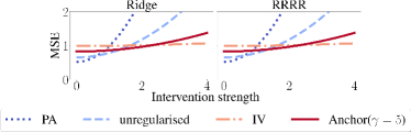
Figure 6: Experiments in high-dimensional setting with $d=p=300$ and $n=200$. We can see that both Multi-output Ridge Regression and Reduced rank Ridge Regression are optimal for a wide range of perturbation strength.

Non-gaussian noise experiments

To assess the robustness of our results presented in paragraph 6.1, we conducted the same toy model experiments with noise $\varepsilon_{A}$, $\varepsilon_{H}$, $\varepsilon_{X}$, and $\varepsilon_{Y}$ following an exponential distribution (Fig. 7.A) and a gamma distribution (Fig. 7.B) with scales $1$.

As observed in Fig. 7, anchor-regularised models remain optimal for a wide range of perturbation strengths, except for anchor-regularised CCA. The behavior of anchor-regularised CCA is explained by its incompatibility with anchor regularisation.

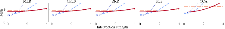
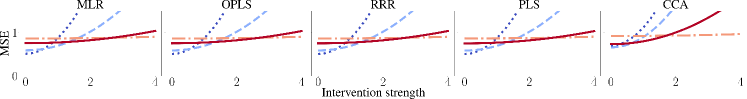
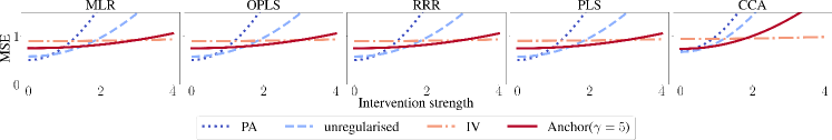
Figure 7: Similar experiments as in 6.1 with noise sampled from non-gaussian distributions. (Top) Exponential distribution of scale$1$, (Middle) Poisson distribution of parameter $1$, (Bottom) Uniform distribution between $-2$ and $2$. We see that all the anchor-compatible algorithms are robust to increasing perturbation strength.

Figure 8: Experiment for anchor confounding $X$ and $Y$. We can see that all algorithms present a very robust behavior to increasing perturbation strength (even CCA which is not anchor-compatible).

Confounding anchor experiment

We also reproduced experiments from equation 12 in Rothenhäusler et al. [2018] to demonstrate how anchor-regularised MVA algorithms exhibit interesting robustness properties when the anchor has a confounding effect. These results are illustrated in Fig. 8. Here, the training distribution is encapsulated in the following Structural Causal Model (SCM):

$$\begin{split}\varepsilon_{A},\,\varepsilon_{H},\,&\varepsilon_{X},\,\varepsilon_{Y}\sim\mathcal{N}(0,1),\\ A&\leftarrow\varepsilon_{A},\\ H&\leftarrow A+\varepsilon_{H},\\ X&\leftarrow A+H+\varepsilon_{X},\\ Y&\leftarrow\mathbf{W}^{T}X+H+\varepsilon_{Y},\end{split}$$ (27)

with again testing distribution sampled by setting $\varepsilon_{A}\sim\mathcal{N}(0,t)$ where $t$ is the perturbation strength and $\mathbf{W}$ being lower rank.

We can see that all algorithms exhibit robustness properties for a very large range of perturbation strength. It is interesting to note that CCA presents a similar behavior as the anchor-compatible algorithms. It would be interesting to investigate in which specific cases CCA gives robustness properties.

10.2 Hyperparameters selection experiment

The results of the toy model experiments in the high-dimensional setting are obtained as follows. The training data are sampled following the DAG

$$\begin{split}\varepsilon_{A},\,\varepsilon_{H},\,&\varepsilon_{X},\,\varepsilon_{Y}\sim\mathcal{N}(0,1),\\ A&\leftarrow\varepsilon_{A},\\ H&\leftarrow\varepsilon_{H},\\ X&\leftarrow\frac{1}{2}A+H+\varepsilon_{X},\\ Y&\leftarrow 2A+\mathbf{W}^{T}X+H+\varepsilon_{Y},\end{split}$$ (28)

and the testing data are generated by modifying $\varepsilon_{A}$ such that $\varepsilon_{A}\sim\mathcal{N}(0,t)$. The perturbation strength $t$ is set to $2$. We repeat each experiment $B=10$ times by resampling $n=100$ training and validation samples and $n=400$ testing samples of $(A,X,Y)$. Both $A$ and $H$ are one-dimensional, while $X$ and $Y$ are $300$-dimensional. The matrix $\mathbf{W}$ is generated as a low-rank (of rank $\rho$ which is randomly sampled uniformly on $[10,30]$) matrix such that $\mathbf{W}=\mathbf{U}\mathbf{V}$ with $\mathbf{U}\in\mathbb{R}^{d\times\rho}$ and $\mathbf{V}\in\mathbb{R}^{\rho\times p}$. The coefficients of $\mathbf{U}$ and $\mathbf{V}$ are sampled uniformly between $1$ and $3$ and are normalised such that their sum is $1$. Hyperparameters $\alpha$ ranging from $1$ to $10^{5}$ are chosen from a logarithmic scale with $20$ candidates, while $\rho$ ranges from $10$ to $30$ linearly with $10$ candidates, and $\gamma$ ranges from $1$ to $10^{4}$ logarithmically with $10$ candidates. Performance, measured in terms of Mean Squared Error and Mean correlation between anchor variable and residuals, is evaluated on a validation set (not seen during training) and a perturbed testing set. We illustrate the results by selecting the optimal rank for each pair $(\gamma,\alpha)$ (see Figure 3). Optimal parameters are chosen to minimize different objectives: for RRRR, parameters $(\alpha,\rho)$ that minimize training MSE are selected, while for A-RRRR, a convex combination of correlation between anchor and residuals ($g_{1}(\gamma,\alpha,\rho)$) and MSE ($g_{2}(\gamma,\alpha,\rho)$) at training is minimized, i.e., $(\gamma,\alpha,\rho)=\operatorname{\text{argmin}}\sum_{i=1}^{2}w_{i}\frac{g_{i}(\gamma,\alpha,\rho)}{\eta_{i}}$, where $\eta_{1}$ and $\eta_{2}$ rescale the two objectives. In Figure 3, we present the results for optimal RRRR and A-RRRR with weights $w_{1}=0.1$ and $w_{2}=0.9$, emphasizing independence of anchor and residuals.

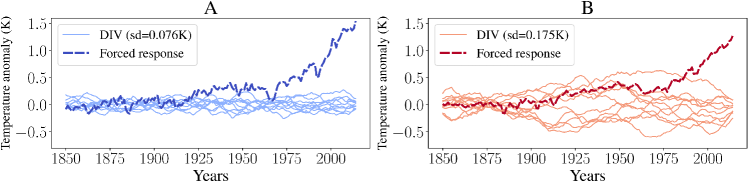
Figure 9: DIV and global forced response for a "low-variability" model (CESM2) (A) and for a "high-variability" model (CNRM-CM6-1) (B).

11 Details of real-world experiment

Optimal fingerprint for detection of forced warming

In D&A studies, the optimal fingerprinting process involves several steps. Firstly, the response of the climate system to an external forcing is extracted using a statistical learning model to predict the forced climate response, denoted as $Y^{\text{forced}}_{\text{mod}}$. This is achieved by utilising spatial predictors from a gridded field of climate variables $X_{\text{mod}}$, following the regression equation:

$$Y_{\text{mod}}^{\text{forced}}=X_{\text{mod}}\beta+\beta_{0}+\varepsilon.$$ (29)

Here, the spatial fingerprint is represented by the regression coefficient $(\beta,\beta_{0})$. Subsequently, a detection metric is obtained by projecting observations ($X_{\text{obs}}$) and unforced simulations ($X_{\text{cntl}}$) (known as control scenarios) onto the extracted fingerprint $\hat{\beta}$. Practically, as multiple members and models are available for the unforced scenario, a distribution for $X_{\text{mod}}^{\text{cntl}}\hat{\beta}+\hat{\beta}_{0}$ can be obtained. Then, it is tested whether $X_{\text{obs}}\hat{\beta}+\hat{\beta}_{0}$ lies within the same distribution. If the test is rejected, a forced response is detected.

From Global to Regional

Moving from a global to regional scale presents challenges in D&A studies. One of the current challenges is transitioning from detecting a global forced response to a regional or local forced response. This is because climate variability magnitude is larger at regional scales, and even larger at a local scale, leading to a lower signal-to-noise ratio of the forced warming response. As the signal-to-noise ratio is in this case much lower, it becomes much more challenging to detect the forced signal. Additionally, different climate models and observations exhibit different patterns of internal variability at regional scales, necessitating the training of statistical learning models robust to potential distribution shifts in internal variability.

Robustness to multidecadal internal variability

The ability to detect forced warming in Detection and Attribution studies is highly influenced by the level of internal variability [see Parsons et al., 2020]. For instance, the observed 40-year Global Mean Temperature (GMT) trend of 0.76°C for the period $1980-2019$ would exceed the standard deviation of natural internal variability in CMIP5 and CMIP6 archive models classified as "low-variability" by a factor of $5$ or more [see Fig. 1B in Sippel et al., 2021]. However, for "high-variability" models, this trend exceeds the standard deviation only by a factor of $2$. This becomes evident when comparing models with "low-variability" (Figure 9 A) to those with "high-variability" (Figure 9 B), where it is less clear that internal variability alone could generate the Global Mean Temperature. This discrepancy poses a significant challenge, as in the former case, the observed warming has an extremely low probability of being generated by internal variability alone. Conversely, in the latter case, the rejection of the hypothesis that current temperature trends are solely attributable to internal variability is less robust. For this reason, it is important to develop tests that are robust to changes in the magnitude of internal variability, particularly with the increasing magnitude of DIV. Assuming the DAG depicted in Figure 10, anchor regularisation emerges as a suitable approach, enabling robust estimation robust to DIV increase.

Figure 10: DAG considered for detection of forced warming response as proposed in Sippel et al. [2021].

Climate models

In this experiment, we utilised $7$ climate models from the CMIP5 and CMIP6 archives, each having at least $8$ members. The selection of these models was primarily practical, based on our access to them and their suitability for the train/test split procedure based on DIV magnitude.

Table 2: Climate models used in this work, their number of members, associated DIV magnitude and corresponding set (train or test).

Model	CMIP	$\sharp$members	DIV mag.	Set
CCSM4	5	8	0.052	Train
NorCMP1	6	30	0.064	Train
CESM2	6	11	0.076	Train
HadCM3	5	10	0.072	Train
CNRM-CM6-1	6	30	0.175	Test
CNRM-ESM2-1	6	10	0.174	Test
IPSL-CM6A-LR	6	32	0.141	Test

Results

Table 3: Metrics for RRRR, and they anchor-regularised version with $\gamma=5$ and $\gamma=100$. We can see that both anchor-regularised approaches outperformed unregularised RRRR in term of $R^{2}$ score and mean correlation of residuals with DIV.

	Test		Train
	$R^{2}$	Mean correlation	$R^{2}$	Mean correlation
RRRR	0.506	0.419	0.510	0.157
A-RRRR ($\gamma=5)$	0.537	0.248	0.500	0.120
A-RRRR ($\gamma=100)$	0.533	0.123	0.487	0.096

The anchor-regularised version of RRRR generally exhibits superior performance compared to its unregularised counterpart (refer to Table 3 and Figure 12), both in terms of prediction performance (measured via $R^{2}$) and correlation between residuals and DIV at testing time. Notably, these results are achieved at a lower training time cost in terms of $R^{2}$, particularly when utilising $\gamma=5$. This trade-off between performance during training and testing becomes clear when looking at the pareto front emerging (Figure  11) when considering different $\gamma$ values for optimal hyperparameters $(\alpha,\rho)$ selected via the validation procedure detailed earlier. We can see that selecting $\gamma$ such as it minimize an equally weighted ($\gamma 0.5/0.5)$ objectives (prediction performances and correlation between residuals and DIV) lead to a very small decrease during training but induce strong robustness (being close to optimal) at testing in terms of predicting performance.

Regarding the spatial patterns of prediction performance, anchor-regularised RRRR outperforms the unregularised version, particularly in the northern hemisphere and notably at the North Pole, where internal climate variability is significantly higher than closer to the equator. It also exhibits superior performance in northern regions where unregularised RRRR performs poorly, albeit with suboptimal results. Conversely, it demonstrates slightly better performance in the southern hemisphere, especially in regions where the DIV and the residuals exhibit anticorrelation (e.g., central Africa and the southern region of South America). In terms of the correlation between DIV and residuals, anchor-regularised RRRR outperforms the unregularised version across most regions, except for central Africa and the southern regions of South America, where residuals and DIV exhibit anticorrelation. On average, it reduces the correlation between residuals and DIV by more than $15\%$ for $\gamma=5$ and close to $30\%$ for $\gamma=100$.

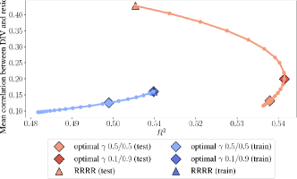
Figure 11: Pareto front for A-RRRR with optimal $\alpha$, $\rho$, and $\gamma\in[1,10^{2}]$ with optimal $\gamma$ of $0.5/0.5$ $0.1/0.9$ weighted objectives.

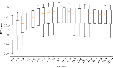
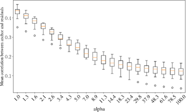
Figure 12: (Left) $R^{2}$ scores (averaged uniformly). (Right) Mean correlation between DIV and residuals for different values of $\gamma$.

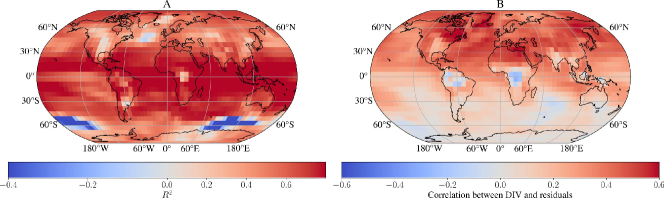
Figure 13: A-RRRR ($\gamma=5$) scores. (A) $R^{2}$ scores. (B) Correlation between DIV and residuals.

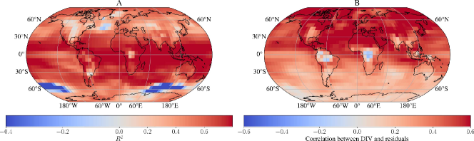
Figure 15: Unregularised RRRR scores. (A) $R^{2}$ scores. (B) Correlation between DIV and residuals.

References

- Abdi [2010] H. Abdi. Partial least squares regression and projection on latent structure regression (PLS regression). Wiley Interdisciplinary Reviews: Computational Statistics, 2:97–106, 01 2010.
- Arenas-Garcia et al. [2013] J. Arenas-Garcia, K. B. Petersen, G. Camps-Valls, and L. K. Hansen. Kernel multivariate analysis framework for supervised subspace learning: A tutorial on linear and kernel multivariate methods. IEEE Signal Processing Magazine, 30(4):16–29, 2013.
- Arenas-García and Gómez-Verdejo [2015] J. Arenas-García and V. Gómez-Verdejo. Sparse and kernel OPLS feature extraction based on eigenvalue problem solving. Pattern Recognition, 48, 05 2015.
- Arjovsky et al. [2020] M. Arjovsky, L. Bottou, I. Gulrajani, and D. Lopez-Paz. Invariant risk minimization, 2020.
- Borchani et al. [2015] H. Borchani, G. Varando, C. Bielza, and P. Larranaga. A survey on multi-output regression. Wiley Interdisciplinary Reviews: Data Mining and Knowledge Discovery, 5, 07 2015. doi: 10.1002/widm.1157.
- Bowden and Turkington [1990] R. J. Bowden and D. A. Turkington. Instrumental variables. Cambridge university press, 1990.
- Bühlmann [2020] P. Bühlmann. Invariance, causality and robustness. ArXiv, 2020.
- Bühlmann and Van De Geer [2011] P. Bühlmann and S. Van De Geer. Statistics for high-dimensional data: methods, theory and applications. Springer Science & Business Media, 2011.
- Candes and Tao [2007] E. Candes and T. Tao. The dantzig selector: Statistical estimation when p is much larger than n. The Annals of Statistics, 35(6):2313 – 2351, 2007.
- Chernozhukov et al. [2017] V. Chernozhukov, D. Chetverikov, M. Demirer, E. Duflo, C. Hansen, and W. Newey. Double/debiased/neyman machine learning of treatment effects. American Economic Review, 107(5):261–65, May 2017.
- Cheung et al. [2017] A. H. Cheung, M. E. Mann, B. A. Steinman, L. M. Frankcombe, M. H. England, and S. K. Miller. Comparison of low-frequency internal climate variability in CMIP5 models and observations. Journal of Climate, 30(12):4763–4776, 2017.
- Cortés-Andrés et al. [2022] J. Cortés-Andrés, G. Camps-Valls, S. Sippel, E. Székely, D. Sejdinovic, E. Diaz, A. Pérez-Suay, Z. Li, M. Mahecha, and M. Reichstein. Physics-aware nonparametric regression models for earth data analysis. Environmental Research Letters, 17(5):054034, 2022.
- Csurka [2017] G. Csurka. Domain Adaptation in Computer Vision Applications. Springer, 01 2017.
- DelSole [2006] T. DelSole. Low-frequency variations of surface temperature in observations and simulations. Journal of Climate, 19(18):4487–4507, 2006.
- Deser et al. [2020] C. Deser, F. Lehner, K. Rodgers, T. Ault, T. Delworth, P. DiNezio, A. Fiore, C. Frankignoul, J. Fyfe, D. Horton, J. Kay, R. Knutti, N. Lovenduski, J. Marotzke, K. McKinnon, S. Minobe, J. Randerson, J. Screen, I. Simpson, and M. Ting. Insights from earth system model initial-condition large ensembles and future prospects. Nature Climate Change, 10:277–286, 04 2020.
- Esfahani and Kuhn [2015] P. Esfahani and D. Kuhn. Data-driven distributionally robust optimization using the Wasserstein metric: Performance guarantees and tractable reformulations. Mathematical Programming, 171, 05 2015.
- Eyring et al. [2016] V. Eyring, S. Bony, G. A. Meehl, C. A. Senior, B. Stevens, R. J. Stouffer, and K. E. Taylor. Overview of the Coupled Model Intercomparison Project Phase 6 (CMIP6) experimental design and organization. Geoscientific Model Development, 9(5):1937–1958, May 2016.
- Girosi et al. [1995] F. Girosi, M. Jones, and T. Poggio. Regularization theory and neural networks architectures. Neural computation, 7(2):219–269, 1995.
- Hastie et al. [2009] T. Hastie, R. Tibshirani, J. H. Friedman, and J. H. Friedman. The elements of statistical learning: data mining, inference, and prediction, volume 2. Springer, 2009.
- Hegerl et al. [1996] G. C. Hegerl, H. von Storch, K. Hasselmann, B. D. Santer, U. Cubasch, and P. D. Jones. Detecting greenhouse-gas-induced climate change with an optimal fingerprint method. Journal of Climate, 9(10):2281–2306, 1996.
- Izenman [1975] A. J. Izenman. Reduced-rank regression for the multivariate linear model. Journal of Multivariate Analysis, 5(2):248–264, 1975.
- Kellenberger et al. [2021] B. Kellenberger, O. Tasar, B. Bhushan Damodaran, N. Courty, and D. Tuia. Deep Domain Adaptation in Earth Observation, chapter 7, pages 90–104. John Wiley & Sons, Ltd, 2021.
- Kociuba and Power [2015] G. Kociuba and S. B. Power. Inability of CMIP5 models to simulate recent strengthening of the walker circulation: Implications for projections. Journal of Climate, 28(1):20–35, 2015.
- Kook et al. [2022] L. Kook, B. Sick, and P. Bühlmann. Distributional anchor regression. Statistics and Computing, 2022.
- Li et al. [2022] Z. Li, A. Pérez-Suay, G. Camps-Valls, and D. Sejdinovic. Kernel dependence regularizers and gaussian processes with applications to algorithmic fairness. Pattern Recognition, 132:108922, 2022.
- Mcgregor et al. [2018] S. Mcgregor, M. Stuecker, J. Kajtar, M. England, and M. Collins. Model tropical atlantic biases underpin diminished pacific decadal variability. Nature Climate Change, 8, 06 2018.
- Mukherjee and Zhu [2011] A. Mukherjee and J. Zhu. Reduced rank ridge regression and its kernel extensions. Statistical Analysis and Data Mining: The ASA Data Science Journal, 4(6):612–622, 2011.
- Namkoong and Duchi [2016] H. Namkoong and J. C. Duchi. Stochastic gradient methods for distributionally robust optimization with f-divergences. In Advances in Neural Information Processing Systems, volume 29. Curran Associates, Inc., 2016.
- Newey and Powell [2003] W. K. Newey and J. L. Powell. Instrumental variable estimation of nonparametric models. Econometrica, 71(5):1565–1578, 2003.
- Oberst et al. [2021] M. Oberst, N. Thams, J. Peters, and D. Sontag. Regularizing towards causal invariance: Linear models with proxies. In International Conference on Machine Learning, pages 8260–8270. PMLR, 2021.
- Parsons et al. [2020] L. A. Parsons, M. K. Brennan, R. C. Wills, and C. Proistosescu. Magnitudes and spatial patterns of interdecadal temperature variability in CMIP6. Geophysical Research Letters, 47(7):e2019GL086588, 2020.
- Peters et al. [2016] J. Peters, P. Bühlmann, and N. Meinshausen. Causal inference by using invariant prediction: Identification and confidence intervals. Journal of the Royal Statistical Society Series B: Statistical Methodology, 78(5):947–1012, 10 2016. ISSN 1369-7412.
- Peters et al. [2017] J. Peters, D. Janzing, and B. Schlkopf. Elements of Causal Inference: Foundations and Learning Algorithms. The MIT Press, 2017. ISBN 0262037319.
- Po-Chedley et al. [2022] S. Po-Chedley, J. Fasullo, N. Siler, Z. Labe, E. Barnes, C. Bonfils, and B. Santer. Internal variability and forcing influence model-satellite differences in the rate of tropical tropospheric warming. Proceedings of the National Academy of Sciences of the United States of America, 119:e2209431119, 11 2022.
- Rothenhäusler et al. [2018] D. Rothenhäusler, P. Bühlmann, N. Meinshausen, and J. Peters. Anchor regression: Heterogeneous data meet causality. Journal of the Royal Statistical Society: Series B (Statistical Methodology), 83, 01 2018.
- Shen et al. [2021] Z. Shen, J. Liu, Y. He, X. Zhang, R. Xu, H. Yu, and P. Cui. Towards out-of-distribution generalization: A survey. ArXiv, abs/2108.13624, 2021.
- Shi and Xu [2023] W. Shi and W. Xu. Learning nonlinear causal effect via kernel anchor regression. In Proceedings of the Thirty-Ninth Conference on Uncertainty in Artificial Intelligence, volume 216 of Proceedings of Machine Learning Research, pages 1942–1952. PMLR, 31 Jul–04 Aug 2023.
- Sippel et al. [2019] S. Sippel, N. Meinshausen, A. Merrifield, F. Lehner, A. G. Pendergrass, E. Fischer, and R. Knutti. Uncovering the forced climate response from a single ensemble member using statistical learning. Journal of Climate, 32(17):5677–5699, 2019.
- Sippel et al. [2021] S. Sippel, N. Meinshausen, E. Székely, E. Fischer, A. G. Pendergrass, F. Lehner, and R. Knutti. Robust detection of forced warming in the presence of potentially large climate variability. Science Advances, 7(43):eabh4429, 2021.
- Sugiyama and Kawanabe [2012] M. Sugiyama and M. Kawanabe. Machine learning in non-stationary environments: Introduction to covariate shift adaptation. MIT press, 2012.
- Sun et al. [2009] L. Sun, S. Ji, S. Yu, and J. Ye. On the equivalence between canonical correlation analysis and orthonormalized partial least squares. In Proceedings of the 21st International Joint Conference on Artificial Intelligence, IJCAI’09, page 1230–1235, San Francisco, CA, USA, 2009. Morgan Kaufmann Publishers Inc.
- Székely et al. [2022] E. Székely, S. Sippel, N. Meinshausen, G. Obozinski, and R. Knutti. Robust detection and attribution of climate change under interventions, 12 2022.
- Taylor et al. [2011] K. E. Taylor, R. J. Stouffer, and G. A. Meehl. An overview of CMIP5 and the experiment design. Bulletin of the American Meteorological Society, 93(4):485–498, 2011. Publisher: American Meteorological Society.
- Tibshirani [1996] R. Tibshirani. Regression shrinkage and selection via the lasso. Journal of the Royal Statistical Society. Series B (Methodological), 58(1):267–288, 1996.
- Tuia et al. [2016] D. Tuia, C. Persello, and L. Bruzzone. Domain adaptation for the classification of remote sensing data: An overview of recent advances. IEEE Geoscience and Remote Sensing Magazine, 4(2):41–57, 2016.
- Zhang et al. [2021] H. Zhang, N. Dullerud, L. Seyyed-Kalantari, Q. Morris, S. Joshi, and M. Ghassemi. An empirical framework for domain generalization in clinical settings. In Proceedings of the Conference on Health, Inference, and Learning, CHIL ’21, page 279–290, New York, NY, USA, 2021. Association for Computing Machinery.
- Zhou et al. [2023] K. Zhou, Z. Liu, Y. Qiao, T. Xiang, and C. C. Loy. Domain generalization: A survey. IEEE Trans. Pattern Anal. Mach. Intell., 45(4):4396–4415, Apr. 2023.
- Zhuang et al. [2021] F. Zhuang, Z. Qi, K. Duan, D. Xi, Y. Zhu, H. Zhu, H. Xiong, and Q. He. A comprehensive survey on transfer learning. Proceedings of the IEEE, 109(1):43–76, Jan. 2021.