Schema-Based Query Optimisation for Graph Databases

Abstract.

Recursive graph queries are increasingly popular for extracting information from interconnected data found in various domains such as social networks, life sciences, and business analytics. Graph data often come with schema information that describe how nodes and edges are organized. We propose a type inference mechanism that enriches recursive graph queries with relevant structural information contained in a graph schema. We show that this schema information can be useful in order to improve the performance when evaluating acylic recursive graph queries. Furthermore, we prove that the proposed method is sound and complete, ensuring that the semantics of the query is preserved during the schema-enrichment process.

1. Introduction

The creation, utilisation and, most importantly, analysis of highly interconnected data has become pervasive in various domains, including social media, astronomy, chemistry, bio-informatics, transportation networks and semantics associations (criminal investigation) (Bell et al., 2009; Barrett et al., 2000; Sheth et al., 2005; Yang et al., 2020). Graph databases have become appealing for modeling, managing and analysing highly interconnected data (Sharma et al., 2021; Alotaibi et al., 2021).

Discovering complex relationships between graph-structured data requires expressive graph query languages to use recursion to navigate paths connecting nodes in a graph database (Jachiet et al., 2020; Duschka et al., 2000). Therefore, the design of contemporary graph query languages is based on formalisms such as regular path queries (RPQ), two-way regular path queries (2RPQ) and nested regular expressions (NRE) along with their extensions such as conjunctive two-way regular path queries (C2RPQ) (Calvanese et al., 1999), union of conjunctive two-way regular path queries (UC2RPQ) (Bonifati et al., 2018; Angles et al., 2017), conjunctive nested regular expressions (CNRE) (Barceló et al., 2013; Libkin et al., 2018), XPath for graph databases (GXPath) (Vrgoc, 2014; Libkin et al., 2013) and more recently conjunctive queries and union of conjunctive queries extended with Tarski’s algebra (CQT/UCQT) (Sharma et al., 2021). These foundations form the basis of languages such as SPARQL (Hogan and Hogan, 2020), Cypher (Francis et al., 2018) and PGQL (van Rest et al., 2016). Furthermore, projects such as ISO/IEC 39075  and Linked Data Benchmark Council  (LDBC) are working towards creating a standard query language for graph databases. At the core of all these graph query languages is recursion. It is essential to perform complex navigation and data extraction from the graph.

Furthermore, graph data often follow a certain organization, structural patterns, or even sets of constraints on the admissible graph shapes. Such knowledge may be left implicit or made explicit by the means of a so-called graph schema specification. In an ongoing standardization effort, PG-Schema (Angles et al., 2023) and PG-Keys (Angles et al., 2021) have been proposed to serve as a reference graph schema language for graph databases.

One fundamental idea of the work presented in this paper is to leverage the schema constraints in order to improve query evaluation. Intuitively, we conjecture that taking advantage of the constraints expressed in a schema can be useful to reduce the amounts of graph data involved when evaluating a query. This research proposes a schema-based query rewriting approach to optimize graph queries. We use a basic yet expressive graph schema formalism (based on (Angles et al., 2023)) to express graph constraints. We consider graph queries expressed in the formalism of UCQT. We propose a type inference method for injecting relevant schema information into the query and produce a schema-aware UCQT variant that is semantically equivalent.

The optimization of recursive queries (even independently from schema constraints) is already known to be significantly more challenging than in the non-recursive setting (Nguyen and Kim, 2017; Yakovets et al., 2015; Jachiet et al., 2020). Extensions to classical relational algebra have been proposed to support recursion (Agrawal, 1988; Gomes-Jr et al., 2015; Yakovets et al., 2015; Leeuwen et al., 2022). As a result, many graph database engines use the query optimisation techniques developed for relational databases (Sun et al., 2015; Shanmugasundaram et al., 1999; Jindal et al., 2014; Xirogiannopoulos et al., 2017). Numerous optimisation techniques have been developed (Meimaris et al., 2017; Neumann and Moerkotte, 2011; Bornea et al., 2013; Jachiet et al., 2020) to optimise recursive graph queries independently from the schema.

However, due to the schema optional nature of contemporary graph databases (Sharma and Sinha, 2022), earlier schema-based methods that have been researched in other settings for recursive queries have been largely ignored. Examples of such earlier methods include static query analyses for Datalog (Bonatti, 2004; Calvanese et al., 1998; Calvanese et al., 2005), semi-structured (Deutsch and Tannen, 2001; Calvanese et al., 1998; Florescu et al., 1998) databases and XML (Benedikt et al., 2008; Lakshmanan et al., 2004; Geerts and Fan, 2005; Genevès and Layaïda, 2006) databases. While these works are essentially of theoretical nature, they can still bring useful insights for schema-based graph query analyses and optimization.

The main contributions of this research work are:

Schema-based approach for query rewriting: we propose a type inference mechanism that uses structural information stored in a graph schema to rewrite queries expressed in the formalism of UCQT. In particular, the type inference mechanism enriches the edge label-based navigational graph queries with additional information related to node labels. This approach aims at reducing the size of intermediate subquery results in order to improve the overall query run time. The approach assists in optimising recursive graph queries and, in some cases, eliminates costly transitive closure operations in the presence of a graph schema. The soundness and completeness of type inference ensure that the semantics of the query is preserved during the process.

Prototype implementation: we have developed a prototype implementation to demonstrate the practical application of the schema-based approach. The prototype primarily focuses on translating the schema-based rewritten query into recursive relational algebra. We use a relational database as a backend. Therefore, we also demonstrate the representation of the graph database as a relational database, enabling efficient querying using the schema-based approach.

Experimental evaluation: in order to empirically evaluate the effectiveness of the approach, we conduct experiments on property graphs and knowledge graphs. We use the LDBC social network benchmark dataset to conduct experiments on property graphs, while the YAGO data set is used to conduct experiments on knowledge graphs. We use third-party queries of varying shapes and types; in particular, we consider acyclic and cyclic shapes, while query types are recursive and non-recursive. The experimental analysis suggests that the proposed schema-based approach is effective for acyclic-shaped recursive graph queries.

Organisation: We present preliminary concepts related to graph databases in Sec. 2, including schemas and the UCQT graph query language. The main contribution to schema-based query rewriting is presented in Sec. 3, where we present an inference system to enrich queries with annotations deduced from the schema. The prototype implementation is presented in Sec. 4, where we describe the overall system architecture. We then report on empirical evaluation results in Sec. 5, where we also consider several relational database systems. Finally, we discuss related works in Sec. 6 before concluding in Sec. 7.

2. Graph DATABASES

We present a few basic definitions related to graph databases. In particular, we define the notions of graph schema, graph database, schema database consistency and graph queries. These notions are vital for schema-based query rewriting. Furthermore, we use the graph database representation of the YAGO data set as a running example to illustrate various definitions present in subsequent sections.

2.1. Graph Schema

A graph schema is a directed pseudo multigraph: a graph in which loops on nodes and multiple directed edges between two nodes are permitted. A graph schema captures the structural and properties-based restrictions in a graph database, with nodes representing entities and edges representing relationships between entities. In graph schemas, nodes and edges are labeled, and properties associated with nodes are expressed in the form of key-type pairs. Let $\mathsf{L}_{\mathsf{N}}$ be a finite set of node labels and $\mathsf{L}_{\mathsf{E}}$ be a finite set of edge labels such that $\mathsf{L}_{\mathsf{N}}\cap\mathsf{L}_{\mathsf{E}}=\emptyset$. Let $\mathsf{K}_{\mathsf{S}}$ be a set of keys (for example: id, name, age), and $\mathsf{T}$ be a finite set of data types (for example: String, Integer, Date). We define a finite set of properties $\mathsf{P}_{\mathsf{S}}$ such that $\mathsf{P}_{\mathsf{S}}\subseteq(\mathsf{K}_{\mathsf{S}}\times\mathsf{T})$.

Figure 1. Sample graph schema for YAGO dataset.

Definition 0 (Graph Schema).

A graph schema is a tuple $\mathsf{S}=(\mathsf{N}_{\mathsf{S}},\mathsf{E}_{\mathsf{S}},\mathsf{L}_{\mathsf{N}},\mathsf{L}_{\mathsf{E}},\mathsf{P}_{\mathsf{S}},\lambda_{\mathsf{S}},\eta_{\mathsf{S}},\xi_{\mathsf{S}},\Delta_{\mathsf{S}})$ where,

• $\mathsf{N}_{\mathsf{S}}$ and $\mathsf{E}_{\mathsf{S}}$ are finite set of nodes and edges such that $\mathsf{N}_{\mathsf{S}}\cap\mathsf{E}_{\mathsf{S}}=\emptyset$.

• $\lambda_{\mathsf{S}}:\mathsf{E}_{\mathsf{S}}\rightarrow\mathsf{N}_{\mathsf{S}}\times\mathsf{N}_{\mathsf{S}}$ is a function which maps all edges to source and target nodes.

• $\eta_{\mathsf{S}}:\mathsf{N}_{\mathsf{S}}\rightarrow\mathsf{L}_{\mathsf{N}}$ is a function which maps all nodes to the set of node labels.

• $\xi_{\mathsf{S}}:\mathsf{E}_{\mathsf{S}}\rightarrow\mathsf{L}_{\mathsf{E}}$ is a function which maps all edges to the set of edge labels.

• $\Delta_{\mathsf{S}}:\mathsf{N}_{\mathsf{S}}\rightarrow 2^{\mathsf{P}_{\mathsf{S}}}$ is a function which maps all nodes to all possible subsets of the property set $\mathsf{P}_{\mathsf{S}}$.

Example 0.

Fig. 1 shows a graph schema for the YAGO dataset (Hoffart et al., 2013) consisting of five nodes and seven edges. All edges are labeled and directed; some edges can represent loops on the same nodes. For instance, the edge labeled as isMarriedTo has the same source and target node labeled as PERSON. All nodes are labeled and have properties associated with them. For instance, a node is labeled as AREA and has a property name:String as a key:type pair.

2.2. Graph Database

A graph database is a graph instance that allows modeling real-world entities as labeled nodes and edges, with properties associated with nodes. Let $\mathsf{K}_{\mathsf{D}}$ be an infinite set of keys (for example, id, name, age), $\mathsf{V}$ be a finite set of values (for example, 345, James). We define a function $\Upsilon:\mathsf{V}\rightarrow\mathsf{T}$ that maps values in $\mathsf{V}$ to their respective data types in $\mathsf{T}$. The set of properties associated with the nodes of a graph database are defined as $\mathsf{P}_{\mathsf{D}}$ such that $\mathsf{P}_{\mathsf{D}}\subseteq(\mathsf{K}_{\mathsf{D}}\times\mathsf{V})$ where each $p_{d}\in\mathsf{P}_{\mathsf{D}}$ is a key-value pair and each value has a data type. Formally, a graph database is defined as follows:

Figure 2. An example of YAGO graph database.

Definition 0 (Graph database).

A graph database is a tuple $\mathsf{D}=(\mathsf{N}_{\mathsf{D}},\mathsf{E}_{\mathsf{D}},\mathsf{L}_{\mathsf{N}},\mathsf{L}_{\mathsf{E}},\mathsf{P}_{\mathsf{D}},\lambda_{\mathsf{D}},\eta_{\mathsf{D}},\xi_{\mathsf{D}},\Delta_{\mathsf{D}})$ where,

• $\mathsf{N}_{\mathsf{D}}$ and $\mathsf{E}_{\mathsf{D}}$ are finite set of nodes and edges such that $\mathsf{N}_{\mathsf{D}}\cap\mathsf{E}_{\mathsf{D}}=\emptyset$.

• $\lambda_{\mathsf{D}}:\mathsf{E}_{\mathsf{D}}\rightarrow\mathsf{N}_{\mathsf{D}}\times\mathsf{N}_{\mathsf{D}}$ is a function which maps all edges to source and target nodes.

• $\eta_{\mathsf{D}}:\mathsf{N}_{\mathsf{D}}\rightarrow\mathsf{L}_{\mathsf{N}}$ is a function which maps all nodes to the set of node labels.

• $\xi_{\mathsf{D}}:\mathsf{E}_{\mathsf{D}}\rightarrow\mathsf{L}_{\mathsf{E}}$ is a function which maps all edges to the set of edge labels.

• $\Delta_{\mathsf{D}}:\mathsf{N}_{\mathsf{D}}\rightarrow 2^{\mathsf{P}_{\mathsf{D}}}$ is a function which maps all nodes to all possible subsets of the property set $\mathsf{P}_{\mathsf{D}}$.

Example 0.

Fig. 2 shows an example of a YAGO graph database consisting of seven nodes and nine edges. All nodes are labeled, and have optional properties associated with them. All edges are labeled and can be identified by unique source and target node identifiers using function $\lambda_{\mathsf{D}}$. For instance, edge $(n_{2},n_{1})$ is labeled as owns, with $n_{2}$ as the source and $n_{1}$ as the target node identifier. The node with identifier $n_{2}$ is labeled as PERSON and has name:John and age:28 as properties.

2.3. Schema-database consistency

The notion of schema-database consistency implies that a graph database follows the structural and property based restrictions established by a graph schema. We define a function $\mathcal{SD}:\mathsf{D}\rightarrow\mathsf{S}$ that maps elements in the graph database to at most one element in the graph schema (also known as strict graph schema (Angles et al., 2023)).

Definition 0 (Schema database consistency).

Given a graph database $\mathsf{D}$ and a graph schema $\mathsf{S}$, we say that $\mathsf{D}$ is consistent with $\mathsf{S}$ when there exists a schema-database mapping $\mathcal{SD}$ such that:

• For every node $n_{i}\in\mathsf{D}$ there exists a corresponding node in the schema: $\mathcal{SD}(n_{i})\in\mathsf{S}$, and we have $\eta_{\mathsf{D}}(n_{i})=\eta_{\mathsf{S}}(\mathcal{SD}(n_{i}))$.

• For every edge $e_{i}\in\mathsf{D}$ there exists a corresponding edge in the schema: $\mathcal{SD}(e_{i})\in\mathsf{S}$. Let $(n_{i},n_{j})=\lambda_{\mathsf{D}}(e_{i})$, then we have $\lambda_{\mathsf{S}}(\mathcal{SD}(e_{i}))=(\mathcal{SD}(n_{i}),\mathcal{SD}(n_{j}))$; furthermore, we have $\eta_{\mathsf{D}}(n_{i})=\eta_{\mathsf{S}}(\mathcal{SD}(n_{i}))$, $\eta_{\mathsf{D}}(n_{j})=\eta_{\mathsf{S}}(\mathcal{SD}(n_{j}))$ and $\xi_{\mathsf{D}}(e_{i})=\xi_{\mathsf{S}}(\mathcal{SD}(e_{i}))$.

• For each $n_{i}\in\mathsf{N}_{\mathsf{D}}$ and for each $(k,v)\in\Delta_{\mathsf{D}}(n_{i})$, we have $(k,\Upsilon(v))\in\Delta_{\mathsf{S}}(\mathcal{SD}(n_{i}))$.

Example 0.

By using Def. 2.5, we can observe that the graph database presented in Fig. 2 is consistent with the graph schema shown in Fig. 1. For instance, edge ($n_{2},n_{3}$) is labeled as isMarriedTo; moreover, source and target nodes are labeled as PERSON and follow the property-based restrictions imposed in the YAGO graph schema.

In this study, we only consider graph databases that are consistent with the graph schema; that is, we exclude any database that does not conform to Def. 2.5. Furthermore, we consider graph databases with restrictions, including nodes having zero or more directed edges, single labels associated with nodes and edges; and zero or more properties for each node. We consider that properties are atomic entities and cannot have maps nor lists as data types.

2.4. Querying graph databases

Graph patterns are essential in graph query languages as they assist in defining the structure of data to be extracted from a graph database (Angles et al., 2017; Francis et al., 2023a; Sharma et al., 2021). The core component of a graph pattern is a path expression corresponding to specifying directed edges and/or paths defined over the edge labels of a graph database. To specify path expressions we use the formalism of Tarski’s algebra which is strictly more expressive than other graph query formalisms such as two-way regular path queries (2RPQ) and nested regular expressions (NRE) (Hellings, 2018; Hellings et al., 2017). The grammar of Tarski’s algebra used to formulate a path expression $\phi$ is presented in Fig. 3.

$$\phi::=$$ path expression

$$l_{e}\in\mathsf{L}_{\mathsf{E}}$$ single edge label

$$| \phi_{1}/\phi_{2}$$ concatenation

$$| \phi_{1}\cup\phi_{2}$$ union

$$| \phi_{1}\cap\phi_{2}$$ conjunction

$$| \phi_{1}[\phi_{2}]$$ branch (right)

$$| [\phi_{1}]\phi_{2}$$ branch (left)

$$| -l_{e}$$ reverse

$$| \phi^{+}$$ transitive closure

Figure 3. Tarski’s algebra grammar (adapted from (Hellings, 2018; Sharma et al., 2021)).

Example 0.

Given a graph schema (Fig. 1) and a graph database (Fig. 2) for the YAGO data set, consider $\phi_{1}=[\texttt{owns}]([\texttt{isMarriedTo}]\texttt{livesIn})$ a path expression used to search for all married property owners living in cities. The path expression $\phi_{1}$ first searches for people living in cities using the livesIn edge label. After that, the branching operation on isMarriedTo edge label only serves as an existential node test to select married people. Finally, the branching operation on the owns edge label only selects married people living in cities and owning properties.

Figure 4. Example of a graph pattern.

In our adaptation of Tarski’s algebra, the reverse operation can be used with single-edge labels, as shown in Fig. 3. Notice that it is possible to use the reverse operator in front of general path expressions $\phi$, as this does not offer any additional expressive power compared to the reverse operation on single-edge labels, as stated in (Hellings, 2018). To express graph patterns, we employ the formalism of conjunctive queries and union of conjunctive queries extended with Tarski’s algebra (CQT/UCQT), which is more expressive than other formalisms used for querying graph databases (Sharma et al., 2021).

2.4.1. Syntax of $\texttt{CQT}/\texttt{UCQT}$

Given a graph schema $\mathsf{S}$ and a graph database $\mathsf{D}$, let $\mathcal{V}_{\mathsf{N}}$ be a finite set of node variables and $\mathcal{P}_{\phi}$ be a set of path expressions $\{\phi_{1},\ldots,\phi_{n}\}$, such that each path expression $\phi_{i}\in\mathcal{P}_{\phi}$ is defined over the set of edge labels $\mathsf{L}_{\mathsf{E}}$.

Definition 0 (CQT).

A conjunctive query with Tarski’s algebra is a logical formula in the $\exists,\wedge$-fragment of first order logic, of the form $\mathsf{C}$ = {($h_{1},\ldots,h_{i}$) $|\hskip 3.99994pt\exists$ $(b_{1},$ $\ldots,b_{j})\hskip 3.99994ptr_{1}\wedge\ldots\wedge r_{l}\wedge\hskip 3.99994pta_{1}\wedge\ldots\wedge a_{k}$ } where,

• $\mathsf{H}=\{h_{1},\ldots,h_{i}\}$ is a finite set of head variables. $\mathsf{B}=\{b_{1},\ldots,b_{j}\}$ is a finite set of body variables such that $(\mathsf{B}\cup\mathsf{H})\subseteq\mathcal{V}_{\mathsf{N}}$ and $(\mathsf{B}\cap\mathsf{H})\neq\emptyset$.

• $\mathsf{A}=\{a_{1},\ldots,a_{k}\}$ is a finite set of atomic formulas formed by a labeling function $\eta_{\mathsf{A}}:\mathcal{V}_{\mathsf{N}}\rightarrow(\mathsf{L}_{\mathsf{N}}\cup\epsilon)$ that maps all node variables to node labels in $\mathsf{L}_{\mathsf{N}}$ or to the empty label. These formulas can be of the form e. g. $\eta_{\mathsf{A}}(Y)=\texttt{PERSON}$ to specify that nodes represented by the variable $Y$ must be labeled as PERSON.

• $\mathsf{Rel}\subseteq(\mathcal{V}_{\mathsf{N}}\times\mathcal{P}_{\phi}\times\mathcal{V}_{\mathsf{N}})$ is a finite set of relations where each relation $r_{i}\in\mathsf{Rel}$ either represent directed edge(s) or path(s) connecting two nodes.

Example 0.

The graph pattern in Fig. 4 identifies people living in regions and countries who also own properties. It consists of two relations: (Y, owns, Z) searches for people who own properties. While (Y, livesIn$/$isLocatedIn⁺, M) specifies a path expression to searches for paths that have edges labeled as livesIn followed by an unbounded number of edges labeled as isLocatedIn returning node that either correspond to regions or cities. Both relations share the same node variable Y, specifying that both relations must search for the same person.

$\mathsf{C}_{1}=\big{\{}\texttt{Y}\hskip 5.59998pt|\hskip 5.59998pt\exists(\texttt{Z,M})\hskip 5.59998pt(\texttt{Y,(livesIn /isLocatedIn+)},\texttt{M})\wedge(\texttt{Y,owns,Z})\}$

QUERY 1 Graph pattern in Fig.4 represented as a CQT

Example 0.

Query 1 presents a graph pattern in Fig. 4 expressed as a CQT where Z,M are body variables and Y is a head variable. Relations $(\texttt{Y,owns,Z})$ and $(\texttt{Y,livesIn /isLocatedIn}^{+},\texttt{M})$ describe the structure of the graph pattern.

We extend the CQT query language formalism to the formalism of the union of conjunctive queries with Tarski’s algebra (UCQT) which is analogous to extending the formalism of C2RPQ to UC2RPQ. The formalism of UCQT represents the disjunction of conjunctive queries with Tarski’s algebra. A UCQT query is written as $\mathsf{UC}=\mathsf{H}\leftarrow\{\mathsf{C}_{1}\cup\ldots\cup\mathsf{C}_{n}\}$, where all $\mathsf{C}_{i}$ are union compatible CQT queries, that is, they share the same set of head variables $\mathsf{H}$ (Pérez et al., 2006; Jachiet et al., 2020).

2.4.2. Semantics of $\texttt{CQT}/\texttt{UCQT}$

As discussed in Sec. 2.4, path expressions form the core components for syntactically describing graph patterns as $\texttt{CQT}/\texttt{UCQT}$. We first present the semantics of path expressions $\phi$ that are based on Tarski’s algebra .

$$\llbracket l_{e}\rrbracket_{\mathsf{D}}= \{(n,m)|n\xrightarrow{l_{e}}m\in\mathsf{E}_{\mathsf{D}}\wedge n,m\in\mathsf{N}_{\mathsf{D}}\wedge l_{e}\in\mathsf{L}_{\mathsf{E}}\}$$

$$\llbracket\phi_{1}/\phi_{2}\rrbracket_{\mathsf{D}}= \{(n,m)|\exists z\in\mathsf{N}_{\mathsf{D}}\wedge(n,z)\in\llbracket\phi_{1}\rrbracket_{\mathsf{D}}\wedge(z,m)\in\llbracket\phi_{2}\rrbracket_{\mathsf{D}}\}$$

$$\llbracket\phi_{1}\cup\phi_{2}\rrbracket_{\mathsf{D}}= \llbracket\phi_{1}\rrbracket_{\mathsf{D}}\cup\llbracket\phi_{2}\rrbracket_{\mathsf{D}}$$

$$\llbracket\phi_{1}\cap\phi_{2}\rrbracket_{\mathsf{D}}= \llbracket\phi_{1}\rrbracket_{\mathsf{D}}\cap\llbracket\phi_{2}\rrbracket_{\mathsf{D}}$$

$$\llbracket\phi_{1}[\phi_{2}]\rrbracket_{\mathsf{D}}= \{(n,m)|\exists z\in\mathsf{N}_{\mathsf{D}}\wedge(n,m)\in\llbracket\phi_{1}\rrbracket_{\mathsf{D}}\wedge(m,z)\in\llbracket\phi_{2}\rrbracket_{\mathsf{D}}\}$$

$$\llbracket[\phi_{1}]\phi_{2}\rrbracket_{\mathsf{D}}= \{(n,m)|\exists z\in\mathsf{N}_{\mathsf{D}}\wedge(n,z)\in\llbracket\phi_{1}\rrbracket_{\mathsf{D}}\wedge(n,m)\in\llbracket\phi_{2}\rrbracket_{\mathsf{D}}\}$$

$$\llbracket-l_{e}\rrbracket_{\mathsf{D}}= \{(m,n)|(n,m)\in\llbracket l_{e}\rrbracket_{\mathsf{D}}\}$$

$$\llbracket\phi^{+}\rrbracket_{\mathsf{D}}= \bigcup\limits_{i\geq 1}\llbracket\phi^{i}\rrbracket_{\mathsf{D}},\phi^{k}=(\underbrace{\phi/\ldots/\phi}_{n-\text{times}})\text{ where }1\leq n\leq i.$$

Figure 5. Semantics of Tarski’s algebra (adapted from (Sharma et al., 2021)).

The interpretation of the path expression $\phi$ when evaluated over a graph database $\mathsf{D}$ (represented as $\llbracket\phi\rrbracket_{\mathsf{D}}$) is defined in Fig. 5. The output produced after evaluating a path expression $\phi$ consists of all pairs of nodes (source and target nodes) that are connected by the path $\phi$ in the graph database. The formalism of $\texttt{CQT}/\texttt{UCQT}$ expresses queries of two types: non-recursive graph queries (NQ) and recursive graph queries (RQ). Non-recursive graph queries are restricted $\texttt{CQT}/\texttt{UCQT}$ that do not allow transitive closure, whereas recursive graph queries allow general path expressions with transitive closure.

The semantics of graph query language formalisms are broadly of two types (i) evaluation semantics and (ii) output semantics (Angles et al., 2017; Sharma et al., 2021). The formalism of $\texttt{CQT}/\texttt{UCQT}$ uses homomorphism-based evaluation semantics for non-recursive graph queries (NQ), arbitrary path semantics for recursive graph queries (RQ) and set-based output semantics (Sharma et al., 2021).

3. Schema-Based Query Rewriting

We introduce a method that leverages schema information for query evaluation. Specifically the method rewrites a query so that structural schema information is injected in relevant part of the queries, namely in path expressions. As a preliminary step, we first transform path expressions into a form where redundancies are eliminated. We then present how schema information can be injected into path expressions.
Preliminary path simplifications: The purpose of rewrite rules presented in Fig. 6 is to eliminate redundancies from path expressions in order to simplify queries. These rewrite rules are general in that they apply independently from any particular schema.

$$(\phi^{+})^{+}\rightarrow\phi^{+}\text{ {(R1)}} \phi_{1}^{+}[\phi_{2}^{+}]\rightarrow\phi_{1}^{+}[\phi_{2}]\text{ {(R2)}} \phi_{1}[\phi_{2}/\phi_{3}]\rightarrow\phi_{1}[\phi_{2}[\phi_{3}]]\text{ {(R3)}}$$

$$[\phi_{2}^{+}]\phi_{1}^{+}\rightarrow[\phi_{2}]\phi_{1}^{+}\text{ {(R4)}} [\phi_{2}/\phi_{3}]\phi_{1}\rightarrow[\phi_{2}[\phi_{3}]]\phi_{1}\text{ {(R5)}}$$

Figure 6. Rewrite rules for path expression simplification.

Rule R1 removes the redundant use of transitive closures. Rules R2 and R4 simplify transitive closures within the branching operator since computing full transitive closure in branching expressions is not required (Hellings, 2018; Hellings et al., 2017). Rules R3 and R5 turn path compositions into branching operations when possible, as also done in prior works (Hellings et al., 2017; Hellings, 2018; Hellings et al., 2020, 2023; Jaakkola and Kuusisto, 2023). Correctness of these rules follows immediately from the formal semantics of path expressions, and in particular from the existential semantics of the branching operator defined in Figure 5.

$$\phi_{red}= \texttt{(((owns[isMarriedTo}^{+}\texttt{/livesIn/dealsWith}^{+}\texttt{])/(isLocatedIn}^{+}\texttt{)}^{+}\texttt{)}^{+}\texttt{)}^{+}$$

$$\phi_{opt}= \texttt{((owns[isMarriedTo[livesIn[dealsWith]]]/isLocatedIn}^{+}\texttt{)}^{+}$$

Figure 7. Application of path simplification rules.

Example 0.

In Fig 7, $\phi_{red}$ is a path expression with redundant plus operations and uses the concatenation operation within the branched path expressions. Rule R1 removes redundant plus operations, rule R2 removes plus operation inside branched expressions, and rule R3 replaces concatenation with branching operation in branched expressions. The optimised path expression is presented in Fig. 7 as the path expression $\phi_{opt}$.

3.1. Schema based query rewriting

Path expressions in Tarski’s algebra do not contain any information about node labels. However, given a graph schema, it is possible to use the structure of a path expression to infer information about node labels. This information can then be used to rewrite the query into another more precise one, which would in general return less results than the original one but is equivalent to it, when the queried database conforms strictly to the schema.

3.1.1. Annotated path expressions

We first extend the grammar of Tarski’s algebra to annotate concatenations with node labels: annotated path expressions $\psi$ follow the same grammar as described in Fig. 3 except that concatenation $/$ can be replaced by its annotated version $/_{l_{n}}$ where $l_{n}$ is a node label. The expression $\psi_{1}/_{l_{n}}\psi_{2}$ represents paths which follow $\psi_{1}$, arrive at a node labeled $l_{n}$, and go on from there following $\psi_{2}$. Formally, we define:

$$\llbracket\psi_{1}/_{l_{n}}\psi_{2}\rrbracket_{\mathsf{D}}=\{(n,m)\mid~{} \exists z\in\mathsf{N}_{\mathsf{D}}~{}\eta_{\mathsf{D}}(z)=l_{n}$$

$$\wedge(n,z)\in\llbracket\psi_{1}\rrbracket_{\mathsf{D}}\wedge(z,m)\in\llbracket\psi_{2}\rrbracket_{\mathsf{D}}\}$$

where $\llbracket\cdot\rrbracket$ is defined as in Fig. 5 for the other cases.

Our idea here is that, when querying a database, replacing a plain path expression with a set of annotated ones can help reduce the size of intermediary results by keeping only the relevant data and thus improve efficiency. To determine how these annotations can be added, we use the schema.

3.1.2. Graph schema triples

Given a graph schema $\mathsf{S}$ as in Def. 2.1, we have that for each edge $e_{i}\in\mathsf{E}_{\mathsf{S}}$, there exists a pair of source and target nodes $\lambda_{\mathsf{S}}(e_{i})=(n_{i},n_{j})$. For each such edge, we consider the basic graph schema triple $t_{i}=(l_{n},l_{e},l_{n}^{\prime})$ constituted by the source label, the edge label and the target label, without any information about properties. Formally:

Definition 0.

The set of basic graph schema triples of $\mathsf{S}$, $\mathcal{T}_{b}(\mathsf{S})$, is defined as follows:

$$\mathcal{T}_{b}(\mathsf{S})=\{(l_{n},l_{e},l_{n}^{\prime}))\mid~{} \exists n_{i},n_{j}\in\mathsf{N}_{\mathsf{S}}~{}~{}\exists e_{i}\in\mathsf{E}_{\mathsf{S}}$$

$$\xi_{\mathsf{S}}(e_{i})=l_{e}\wedge\lambda_{\mathsf{S}}(e_{i})=(n_{i},n_{j})$$

$$\wedge\eta_{\mathsf{S}}(n_{i})=l_{n}\wedge\eta_{\mathsf{S}}(n_{j})=l_{n}^{\prime}\}$$

Example 0.

The graph schema as shown in Fig. 1 contains seven edges; therefore, the set associated with the schema contains seven basic graph schema triples $\mathcal{T}_{b}(\mathsf{S})=\{t_{1},\ldots,t_{7}\}$. For instance, the triple $t_{1}$ = (PERSON, owns, PROPERTY) has PERSON as source node label, PROPERTY as target node label and owns as an associated edge label. Similarly, the triple $t_{2}$ = (PROPERTY, isLocatedIn, CITY) has PROPERTY as source node label, CITY as target node label and isLocatedIn as an associated edge label.

Consider the path expression owns. The only triple containing this label is $t_{1}$. If we query a database conforming to our schema, we are able to know that this path expression will only return results conforming to $t_{1}$, in the sense that their source node will be labeled PERSON and their target node PROPERTY.

Basic graph schema triples correspond to path expressions consisting of a single edge label. More generally, we define graph schema triples as follows:

Definition 0.

A graph schema triple is a triple $(l_{n},\psi,l_{n}^{\prime})$ where $l_{n}$ and $l_{n}^{\prime}$ are node labels and $\psi$ an annotated path expression. For a graph schema triple $t$, we write $\texttt{sc}(t),\texttt{eTA}(t)$ and $\texttt{tg}(t)$ respectively the source node label, annotated path expression and target node label.

Given a plain path expression and a graph schema, we can compute a number of graph schema triples which are compatible with the path expression. For example, if we consider the path expression $\texttt{owns}/\texttt{isLocatedIn}$, considering that triples $t_{1}$ and $t_{2}$ from Exp. 3.3 share a common node label PROPERTY, we can build the triple $(\texttt{PERSON},\texttt{owns}/_{\texttt{PROPERTY}}\texttt{isLocatedIn},\texttt{CITY})$. In that example, it is the only triple compatible with the expression.

3.1.3. Path expression and triple compatibility

Figure 8. Inference rules for the path expression-graph schema triple compatibility relation.

The set of triples compatible with a given path expression $\phi$ according to a schema $\mathsf{S}$ can be computed inductively from the sets of triples compatibles with the parts of $\phi$. We do this using inference rules and an auxiliary function.

Definition 0 (path expression-triple compatibility).

Let $\phi$ be a path expression, $\mathsf{S}$ a graph schema and $t$ a graph schema triple. The judgement $\vdash_{\mathsf{S}}{\phi}\colon{t}$ means that under schema $\mathsf{S}$, $\phi$ is compatible with $t$. It is defined inductively by the rules in Fig. 3.1.3, where $\mathcal{T}_{\mathsf{S}}(\phi)$ represents the set of all triples compatible with $\phi$:

$$\mathcal{T}_{\mathsf{S}}(\phi)=\{t\mid\vdash_{\mathsf{S}}{\phi}\colon{t}\}$$

The last rule, TPlus, relies on the auxiliary function $\mathsf{PlC}$, which works on the whole set of triples compatible with $\phi$ at once. This function, defined below, generates two kinds of triples: (a) triples where the path expression is ${\phi}^{+}$ itself, with all annotations dropped, and (b) triples where the path expression does not contain +, the transitive closure operator, anymore. The rationale behind that is that if the schema information allows us to avoid the costly transitive closure, we prefer to do so. However, we do not want to overcomplicate the expression if we cannot avoid the transitive closure operation.

To determine when transitive closure can be avoided, we associate to the set $\mathcal{T}_{\mathsf{S}}(\phi)$ the directed graph whose vertices are the node labels and whose edges are the triples. Any path of length $n$ in that graph yields a triple compatible with $\phi^{n}$ (as we can infer by repeated application of TConcat). Since the meaning of ${\phi}^{+}$ is the union of the $\phi^{n}$ for all $n\geqslant 1$, the set of all (non-empty) paths in the graph corresponds to triples compatible with ${\phi}^{+}$. If this set is finite, we actually define it as the set of triples compatible with ${\phi}^{+}$. If it is infinite, then transitive closure cannot be removed. Since the existence of infinitely many paths is equivalent to the presence of cycles in the graph, we propose the following algorithm for computing $\mathsf{PlC}$:

Definition 0 (Plus Compatibility).

$\mathsf{PlC}(\phi,\mathcal{T})$ is the set of triples resulting of the following:

1. Let $G$ be the directed graph associated with $\mathcal{T}$;

2. Let $K$ be the set of vertices of $G$ which are part of a cycle;

3. Let $R$ be the initially empty result set;

4. For each path $p$ from $A$ to $B$ without cycles in $G$:

   • if any of the vertices of $p$ (including $A$ and $B$) is in $K$, then

     • add to $R$ the triple $(A,{\phi}^{+},B)$

   • else

     • let $\psi$ be the annotated path expression resulting of concatenating all triples in $p$;

     • add to $R$ the triple $(A,\psi,B)$

5. Return $R$.

Example 0.

Consider the path expression $\phi_{4}=\texttt{livesIn}/\texttt{isLocatedIn}^{+}/\texttt{dealsWith}^{+}$, and let $\mathsf{S}$ be the schema of Fig. 1. Table 1 shows the sets of triples associated to $\phi_{4}$ and its three sub-terms $\phi_{1}=\texttt{livesIn}(\texttt{lvIn})$, $\phi_{2}=\texttt{isLocatedIn}^{+}(\texttt{isL}^{+})$ and $\phi_{3}=\texttt{dealsWith}^{+}(\texttt{dw}^{+})$.

For $\phi_{3}$, we have $\mathcal{T}_{\mathsf{S}}(\texttt{dealsWith})=\{(\texttt{COUNTRY},\texttt{dealsWith},\texttt{COUNTRY})\}$. The graph associated to that singleton set has one vertex and one edge which forms a cycle, therefore the transitive closure cannot be eliminated: we have $\mathcal{T}_{\mathsf{S}}(\texttt{dealsWith}^{+})=(\texttt{COUNTRY},\texttt{dealsWith}^{+},\texttt{COUNTRY})$.

For $\phi_{2}$, the set $\mathcal{T}_{\mathsf{S}}(\texttt{isLocatedIn})$ contains 3 triples; the associated graph has 4 vertices (PROPERTY, CITY, REGION and COUNTRY) and 3 edges corresponding to the 3 triples. It contains no cycle, therefore $\mathcal{T}_{\mathsf{S}}(\texttt{isLocatedIn}^{+})$ contains 6 triples, corresponding to the 6 non-empty paths in the graph.

Notice that, while TPlus can yield many triples when it is possible to remove the transitive closure, TConcat on the other hand can drastically reduce their number, so that in the end there is only one triple compatible with $\phi_{4}$.

Table 1. Application of the inference rules of Fig. 3.1.3 to the term $\phi_{4}=\texttt{livesIn}/\texttt{isLocatedIn}^{+}/\texttt{dealsWith}^{+}$.

TERM	TRIPLES	RULE
lvIn	(PER, lvIn, CITY)	TBasic
$\texttt{isL}^{+}$	(PRO, isL, CITY), (CITY, isL, REG),
(REG, isL, CUN), (PRO, isL$/_{\texttt{CITY}}$isL, REG),
(PRO, isL$/_{\texttt{CITY}}$isL$/_{\texttt{REG}}$isL, CUN),
(CITY, isL$/_{\texttt{REG}}$isL, CUN)	TPlus
$\texttt{dw}^{+}$	(CUN, $\texttt{dw}^{+}$, CUN)	TPlus
$\texttt{lvIn}/\texttt{isL}^{+}$	(PER, lvIn$/_{\texttt{CITY}}$isL, REG),
(PER, lvIn$/_{\texttt{CITY}}$isL$/_{\texttt{REG}}$isL, CUN)	TConcat
$\texttt{lvIn}/\texttt{isL}^{+}/\texttt{dw}^{+}$	(PER, lvIn$/_{\texttt{CITY}}$isL$/_{\texttt{REG}}$isL$/_{\texttt{CUN}}$dw+, CUN)	TConcat
CUN = COUNTRY	isL = isLocatedIn, lvIn = livesIn	REG = REGION
PRO = PROPERTY	dw = dealsWith	PER = PERSON

3.1.4. Properties of the compatibility relation

The path expression-triple compatibility relation is defined relative to a schema. Consider now a database conforming to this schema. The compatibility relation enjoys the following properties relative to any such database:

• Soundness, meaning that whenever our path expression $\phi$ is compatible with some triple ${(l_{n},\psi,l_{n}^{\prime})}$, then all pairs of a node labeled $l_{n}$ and a node labeled $l_{n}^{\prime}$ linked, in the database, by a path conforming to $\psi$, are part of the result of $\phi$;

• Completeness, meaning that whenever $\phi$ returns a pair of a node labeled $l_{n}$ and a node labeled $l_{n}^{\prime}$, there exists a triple ${(l_{n},\psi,l_{n}^{\prime})}$, compatible with $\phi$, such that these nodes are linked, in the database, by a path conforming to $\psi$.

These two properties make the initial path expression semantically equivalent to its set of compatible triples, so long as we only consider databases conforming to the schema. Formally:

Theorem 3.8.

Let $\mathsf{S}$ be a graph schema, let $\mathsf{D}$ be a graph database conforming to $\mathsf{S}$ via the schema-database mapping $\mathcal{SD}$, and let $\phi$ be a path expression.

Soundness. Assume $\vdash_{\mathsf{S}}{\phi}\colon{(l_{n},\psi,l_{n}^{\prime})}$ holds for some triple $(l_{n},\psi,l_{n}^{\prime})$. Let $(s,t)\in\llbracket{\psi}\rrbracket_{\mathsf{D}}$ such that $\eta_{\mathsf{D}}(s)=l_{n}$ and $\eta_{\mathsf{D}}(t)=l_{n}^{\prime}$. Then $(s,t)\in\llbracket{\phi}\rrbracket_{\mathsf{D}}$.

Completeness. Let $(s,t)\in\llbracket{\phi}\rrbracket_{\mathsf{D}}$. Then there exists $\psi$ such that $(s,t)\in\llbracket{\psi}\rrbracket_{\mathsf{D}}$ and $\vdash_{\mathsf{S}}{\phi}\colon{(\eta_{\mathsf{D}}(s),\psi_{,}\eta_{\mathsf{D}}(t))}$.

Proof.

Both properties are proved by structural induction on $\phi$. The base cases, where $\phi$ is a single edge label, are a direct consequence of the consistency between $\mathsf{D}$ and $\mathsf{S}$ (def. 2.5) and of the definition of basic graph schema triples (def. 3.2). The inductive cases other than transitive closure are straightforward since the inference rules of Fig. 3.1.3 follow exactly the structure of the semantics defined in Fig. 5. Finally, we detail the case of transitive closure:

Soundness: assume the property holds for $\phi$. Let $(l_{n},\psi,l_{n}^{\prime})\in\mathsf{PlC}(\phi,\mathcal{T}_{\mathsf{S}}(\phi))$ and let $(s,t)\in\llbracket{\psi}\rrbracket_{\mathsf{D}}$ such that $\eta_{\mathsf{D}}(s)=l_{n}$ and $\eta_{\mathsf{D}}(t)=l_{n}^{\prime}$. We have two cases: if $\psi={\phi}^{+}$ then the result is immediate. Otherwise, according to Def. 3.6, it means that there exists a sequence of triples $t_{1},\ldots,t_{n}\in\mathcal{T}_{\mathsf{S}}(\phi)$ such that: $\texttt{sc}(t_{1})=l_{n}$, $\texttt{tg}(t_{i})=\texttt{sc}(t_{i+1})$ for all $i<n$, $\texttt{tg}(t_{n})=l_{n}^{\prime}$, and $\psi$ is the concatenation of $t_{1}\ldots t_{n}$ (i. e. $\psi=\texttt{eTA}(t_{1})/_{\texttt{tg}(t_{1})}\texttt{eTA}(t_{2})/_{\texttt{tg}(t_{2})}\cdots/_{\texttt{tg}(t_{n-1})}\texttt{eTA}(t_{n})$). Since $(s,t)$ is in $\llbracket{\psi}\rrbracket_{\mathsf{D}}$, it means that there is a path in $\mathsf{D}$ from $s$ to $t$ which conforms to $\psi$. Since $\psi$ is the concatenation of $t_{1}\ldots t_{n}$, that path has to be the concatenation of $n$ sub-paths conforming respectively to the triples $t_{1}\ldots t_{n}$. Since each of those triples is compatible with $\phi$, we can use the induction hypothesis for each of them and see that the source-target pair for each one is in $\llbracket{\phi}\rrbracket_{\mathsf{D}}$. It results that $(s,t)$ is in $\llbracket{\phi^{n}}\rrbracket_{\mathsf{D}}$, and therefore in $\llbracket{{\phi}^{+}}\rrbracket_{\mathsf{D}}$.

Completeness: assume the property holds for $\phi$. Let $(s,t)\in\llbracket{{\phi}^{+}}\rrbracket_{\mathsf{D}}$. By definition, there exists $k\geqslant 1$ such that $(s,t)\in\llbracket{\phi^{k}}\rrbracket_{\mathsf{D}}$. This means that there is a sequence $n_{0}\ldots n_{k}$ of nodes in $D$ with $n_{0}=s$ and $n_{k}=t$ such that we have $(n_{i-1},n_{i})\in\llbracket{\phi}\rrbracket_{\mathsf{D}}$ for all $i$ between $1$ and $k$. By induction hypothesis, for each $i$ there is a triple $t_{i}=(\eta_{\mathsf{D}}(n_{i-1}),\psi_{i},\eta_{\mathsf{D}}(n_{i}))$ such that $\vdash_{\mathsf{S}}{\phi}\colon{t_{i}}$ and $(n_{i-1},n_{i})\in\llbracket{\psi_{i}}\rrbracket_{\mathsf{D}}$. Let $G$ and $K$ be the graph and set of vertices defined in Def. 3.6. The sequence $t_{1}\ldots t_{k}$ forms a path from $\eta_{\mathsf{D}}(s)$ to $\eta_{\mathsf{D}}(t)$ in $G$. If this path contains no cycle, then we see from step (4) of Def. 3.6 that $\mathsf{PlC}(\phi,\mathcal{T}_{\mathsf{S}}(\phi))$ contains a triple $(\eta_{\mathsf{D}}(s),\psi,\eta_{\mathsf{D}}(t))$ with $\psi$ equal either to ${\phi}^{+}$ or to the concatenation of $\psi_{1}\ldots\psi_{k}$. In both cases, we have $(s,t)\in\llbracket{\psi}\rrbracket_{\mathsf{D}}$. If the path $t_{1}\ldots t_{k}$ does contain a cycle, say $\eta_{\mathsf{D}}(n_{i})=\eta_{\mathsf{D}}(n_{j})$ with $j>i$, then the sequence $t_{1}\ldots t_{i},t_{j+1}\ldots t_{k}$ is also a path in $G$ without that cycle, and we have $\eta_{\mathsf{D}}(n_{j})\in K$ since $t_{i+1}\ldots t_{j}$ is a cycle in $G$. If that path still contains a cycle, we can reiterate this ‘shortcutting’ until there are none left, and obtain a path from $\eta_{\mathsf{D}}(s)$ to $\eta_{\mathsf{D}}(t)$ without cycles and containing at least one vertex in $K$. Therefore, $\mathsf{PlC}(\phi,\mathcal{T}_{\mathsf{S}}(\phi))$ must contain the triple $(\eta_{\mathsf{D}}(s),{\phi}^{+},\eta_{\mathsf{D}}(t))$, which allows us to conclude since we already have $(s,t)\in\llbracket{{\phi}^{+}}\rrbracket_{\mathsf{D}}$. ∎

3.1.5. Rewritten queries

$$\mathcal{Q}(\alpha,\beta,\phi)=(\emptyset,\emptyset,\{(\alpha,\phi,\beta)\})$$

$$\mathcal{Q}(\alpha,\beta,\psi_{1}/_{l_{n}}\psi_{2})=\text{let $\gamma$ be a fresh variable,}$$

$$\quad\text{let }(\mathsf{B}_{1},\mathsf{A}_{1},\mathsf{Rel}_{1})=\mathcal{Q}(\alpha,\gamma,\psi_{1})\text{ and }(\mathsf{B}_{2},\mathsf{A}_{2},\mathsf{Rel}_{2})=\mathcal{Q}(\gamma,\beta,\psi_{2})$$

$$\quad\text{in }(\mathsf{B}_{1}\cup\mathsf{B}_{2}\cup\{\gamma\},\mathsf{A}_{1}\cup\mathsf{A}_{2}\cup\{\eta_{\mathsf{A}}(\gamma)=l_{n}\},\mathsf{Rel}_{1}\cup\mathsf{Rel}_{2})$$

$$\mathcal{Q}(\alpha,\beta,\psi_{1}[\psi_{2}])=\text{let $\gamma$ be a fresh variable,}$$

$$\quad\text{let }(\mathsf{B}_{1},\mathsf{A}_{1},\mathsf{Rel}_{1})=\mathcal{Q}(\alpha,\beta,\psi_{1})\text{ and }(\mathsf{B}_{2},\mathsf{A}_{2},\mathsf{Rel}_{2})=\mathcal{Q}(\beta,\gamma,\psi_{2})$$

$$\quad\text{in }(\mathsf{B}_{1}\cup\mathsf{B}_{2}\cup\{\gamma\},\mathsf{A}_{1}\cup\mathsf{A}_{2},\mathsf{Rel}_{1}\cup\mathsf{Rel}_{2})$$

$$\mathcal{Q}(\alpha,\beta,[\psi_{1}]{\psi_{2}})=\text{let $\gamma$ be a fresh variable,}$$

$$\quad\text{let }(\mathsf{B}_{1},\mathsf{A}_{1},\mathsf{Rel}_{1})=\mathcal{Q}(\alpha,\gamma,\psi_{1})\text{ and }(\mathsf{B}_{2},\mathsf{A}_{2},\mathsf{Rel}_{2})=\mathcal{Q}(\alpha,\beta,\psi_{2})$$

$$\quad\text{in }(\mathsf{B}_{1}\cup\mathsf{B}_{2}\cup\{\gamma\},\mathsf{A}_{1}\cup\mathsf{A}_{2},\mathsf{Rel}_{1}\cup\mathsf{Rel}_{2})$$

$$\mathcal{Q}(\alpha,\beta,{\psi_{1}}\cap{\psi_{2}})=$$

$$\quad\text{let }(\mathsf{B}_{1},\mathsf{A}_{1},\mathsf{Rel}_{1})=\mathcal{Q}(\alpha,\beta,\psi_{1})\text{ and }(\mathsf{B}_{2},\mathsf{A}_{2},\mathsf{Rel}_{2})=\mathcal{Q}(\alpha,\beta,\psi_{2})$$

$$\quad\text{in }(\mathsf{B}_{1}\cup\mathsf{B}_{2},\mathsf{A}_{1}\cup\mathsf{A}_{2},\mathsf{Rel}_{1}\cup\mathsf{Rel}_{2})$$

Figure 9. Translation of annotated path expressions into CQTs.

We now want to translate graph schema triples into CQT queries. For this, we first observe that the annotated path expressions $\psi$ generated by the rules of Fig. 3.1.3 and Def. 3.6 always obey some syntactic restrictions, namely: no annotations appear under the transitive closure operator, and the union operator never appears, except possibly under transitive closure. Furthermore, the reverse operation only occurs in front of edge labels. These observations allow us to reduce the number of cases in the translation: $\psi$ is either a plain path expression, a concatenation, a branching or a conjunction.

Definition 0 (CQT of a triple).

The translation is defined using a function $\mathcal{Q}(\alpha,\beta,\psi)$, where $\alpha$ and $\beta$ are CQT variables and $\psi$ an annotated path expression, which returns a triple $(\mathsf{B},\mathsf{A},\mathsf{Rel})$ corresponding to a CQT representing $\psi$ with $\mathsf{H}=\{\alpha,\beta\}$ (see Def. 2.8). This function is defined in Fig. 9.

For a given graph schema triple $t=(l_{n},\psi,l_{n}^{\prime})$, we then define the associated CQT as $\mathsf{C}(t)=(\{\alpha,\beta\},\mathsf{B},\mathsf{A}\cup\{\eta_{\mathsf{A}}(\alpha)=l_{n},\eta_{\mathsf{A}}(\beta)=l_{n}^{\prime}\},\mathsf{Rel})$ where $(\mathsf{B},\mathsf{A},\mathsf{Rel})=\mathcal{Q}(\alpha,\beta,\psi)$.

This allows us to associate to any path expression, given a schema $\mathsf{S}$, a UCQTrepresenting the query enriched with schema information:

Definition 0 (schema-enriched query).

Given a path expression $\phi$ and a schema $\mathsf{S}$, the schema-enriched query of $\phi$, $\mathcal{R}_{\mathsf{S}}(\phi)$, is the following UCQT:

$$\mathcal{R}_{\mathsf{S}}(\phi)=\{\alpha,\beta\}\leftarrow\{\bigcup_{t\in\mathcal{T}_{\mathsf{S}}(\phi)}\mathsf{C}(t)\}$$

Thanks to Theorem 3.8, we have that $\phi$ is equivalent to $\mathcal{R}_{\mathsf{S}}(\phi)$ on any database conforming strictly to $\mathsf{S}$.

Example 0.

Consider the path expression $\phi_{4}=\texttt{lvIn}/\texttt{isL}^{+}/\texttt{dw}^{+}$ of Example 3.7. We saw that our inference system derives exactly one triple compatible with it in schema $\mathsf{S}$: (PER, lvIn$/_{\texttt{CITY}}$isL$/_{\texttt{REG}}$isL$/_{\texttt{CUN}}$dw⁺, CUN). Therefore, we can rewrite this expression into:

$$\mathcal{R}_{\mathsf{S}}(\phi_{4})=\{ \alpha,\beta\mid\exists(\gamma,\delta,\zeta)\quad(\alpha,\texttt{lvIn},\gamma)\wedge(\gamma,\texttt{isL},\delta)\wedge(\delta,\texttt{isL},\zeta)$$

$$\wedge(\zeta,\texttt{dw}^{+},\beta)\wedge\eta_{\mathsf{A}}(\alpha)=\texttt{PER}\wedge\eta_{\mathsf{A}}(\beta)=\texttt{CUN}$$

$$\wedge\eta_{\mathsf{A}}(\gamma)=\texttt{CITY}\wedge\eta_{\mathsf{A}}(\delta)=\texttt{REG}\wedge\eta_{\mathsf{A}}(\zeta)=\texttt{CUN}\}$$

We can notice that the rewritten query allows the database engine to avoid computing the transitive closure of isL at all.

4. System Implementation

We analyse the performance of queries augmented with schema information. The approach has been implemented as a system whose architecture is depicted in Figure 10. Our system architecture consists of three main modules (i) Rewriter, (ii) Translator and (iii) Backend.

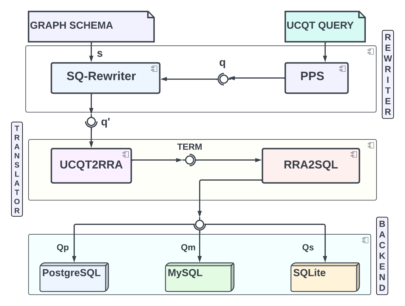
Figure 10. System architecture.

Rewriter:

The rewriter module consists of two components Preliminary Path Simplifier (PPS) and Schema-based Query Rewriter (SQ-Rewriter). The PPS component takes a UCQT query as an input, then applies the preliminary path simplification rules presented in Fig. 6 and produces a simplified UCQT query $q$ as output. The SQ-Rewriter component implements the query rewritings leveraging schema information presented in Section 3 for the UCQT query language (defined in Section 2.4). It takes a UCQT query $q$ and a graph schema $s$ described in the graph schema formalism (using Def. 2.1) as input and generates a schema-aware UCQT query $q^{\prime}$ as output.

Translator:

The translator module compiles a UCQT query into a recursive SQL query that can be executed by a relational database management system (RDBMS). In this process, we apply recursive relational algebra (RRA) optimisations. Specifically, the translator module first uses the UCQT2RRA component to translate UCQT query to a term in recursive relational algebra, and that is further optimised using the $\mu\texttt{-RA}$ system based on the notations and rewritings proposed in (Jachiet et al., 2020). Compared to the path expressions considered in (Jachiet et al., 2020), we consider additional translation rules for translating conjunction and branching operations as shown in Tab. 2.

Table 2. Conjunction and branching translation to RRA.

Path expression	RRA term
$\llparenthesis\phi_{1}\cap\phi_{2}\rrparenthesis=$	$\big{\{}\rho_{n}^{\mathsf{Tr}}\left(\rho_{m}^{\mathsf{Sr}}\left(\rho_{\mathsf{Tr}}^{n}\left(\rho_{\mathsf{Sr}}^{m}\left(\varphi_{1}\right)\right)\bowtie\rho_{\mathsf{Tr}}^{n}\left(\rho_{\mathsf{Sr}}^{m}\left(\varphi_{2}\right)\right)\right)\right)\big{|}\quad\varphi_{1}\in\llparenthesis\phi_{1}\rrparenthesis\wedge\varphi_{2}\in\llparenthesis\phi_{2}\rrparenthesis\big{\}}$
$\llparenthesis\phi_{1}[\phi_{2}]\rrparenthesis=$	$\big{\{}\rho_{m}^{\mathsf{Tr}}\left(\rho_{\mathsf{Tr}}^{m}\left(\varphi_{1}\right)\bowtie\rho_{\mathsf{Sr}}^{m}\left(\pi_{\mathsf{Sr}}\left(\varphi_{2}\right)\right)\right)\big{|}\quad\varphi_{1}\in\llparenthesis\phi_{1}\rrparenthesis\wedge\varphi_{2}\in\llparenthesis\phi_{2}\rrparenthesis\big{\}}$
$\llparenthesis[\phi_{1}]\phi_{2}\rrparenthesis=$	$\big{\{}\rho_{m}^{\mathsf{Sr}}\left(\rho_{\mathsf{Sr}}^{m}\left(\pi_{\mathsf{Sr}}\left(\varphi_{1}\right)\right)\bowtie\rho_{\mathsf{Sr}}^{m}\left(\varphi_{2}\right)\right)\big{|}\quad\varphi_{1}\in\llparenthesis\phi_{1}\rrparenthesis\wedge\varphi_{2}\in\llparenthesis\phi_{2}\rrparenthesis\big{\}}$

Our system architecture priorities modularity, allowing for components such as UCQT2RRA (currently based on the $\mu\texttt{-RA}$ system) to be replaced with other systems such as $\alpha$-extended RA (Agrawal, 1988), $\beta$-RA (Gomes-Jr et al., 2015), WAVEGUIDE (Yakovets et al., 2015), AVANTGRAPH (Leeuwen et al., 2022) and DATALOG based RRA systems (Aref et al., 2015; Leone et al., 2006; Urbani et al., 2016). However, as discussed in (Jachiet et al., 2020; Fejza et al., 2023), the $\mu\texttt{-RA}$ system is superior in query optimisation capabilities.

The optimised RRA term is transformed into a concrete recursive SQL syntax for each RDBMS using the RRA2SQL component. Specifically, the PostgreSQL RDBMS enables the translation of RRA terms into SQL, and the fixpoints can be converted into a recursive view statement. However, MySQL and SQLite RDBMS do not allow using a recursive table more than once within a recursive view statement^,. Therefore, in our concrete SQL translations, we substituted the natural join with an equijoin clause for MySQL and SQLite inside the recursive view statements.

Backend:

In order to evaluate our approach we conduct experiments on three RDBMS, in particular we use PostgreSQL, MySQL and SQLite. In our implementation, we store graph databases in the relational data model by representing the nodes and edges of the graph database in relational tables. For instance, the graph database for YAGO dataset (shown in Fig. 2), the relational representation of graph edges labeled livesIn between two types of nodes, labeled PERSON and CITY, as shown in Fig. 11. One table for each type of node label is created, with a specific column $\mathsf{Sr}$ that serves as a primary key and potentially many other columns for properties. Similarly, one table is created for each type of edge label, with at least two columns $\mathsf{Sr}$ and $\mathsf{Tr}$ that are foreign keys pointing to source and target nodes . Therefore, each row in the node or edge tables represents a node or an edge of the graph database.

Figure 11. Relational representation of nodes and edges.

5. Experiments

We assess the impact on performance of the schema-based approach experimentally with a complete prototype implementation. Concretely, we try to answer the following questions: (i) Does the schema-based approach improve the performance of query evaluation on real and synthetic or benchmark datasets? (ii) Is the impact on performance dependent on the graph querying features of the query? (iii) Are the results consistent across several relational database management systems (RDBMS)?

5.1. Experimental Setup

5.1.1. Datasets

We consider datasets of different nature:

• YAGO (Yago, 2019), which is a real knowledge graph. We use a cleaned version of the real-world dataset YAGO2s (Yago, 2019) in which only nodes with unique identifiers are present. We split the set of RDF triples into multiple edge relations (tables), one for each predicate name. We create a node relation (table) for each node class.

• the Social Network Benchmark (SNB) interactive workload from the Linked Data Benchmark Council (LDBC) (Erling et al., 2015) which is a synthetic reference benchmark for property graphs. Specifically, we used the LDBC-SNB dataset in CSV format provided from (Szárnyas, 2023).

Table 3. Summary of dataset characteristics.

Name	SF	#NR	#ER	#Nodes	#Edges	Size
YAGO	N/A	7	88	98,582	150,391,592	26 GB
	0.1			416,311	2,034,983	0.3 GB
	0.3			1,154,108	6,235,570	0.9 GB
LDBC-SNB	1	8	16	3,966,203	23,056,025	3.3 GB
	3			11,407,480	69,482,982	9.9 GB
	10			36,485,994	231,532,873	33 GB

Table 3 summarises the characteristics of the pre-processed datasets. The YAGO dataset has 98k nodes and 150M edges, with 7 node relations and 88 edge relations. LDBC-SNB uses 8 node relations (NR) and 16 edge relations (ER). LDBC-SNB has property graphs of varying sizes measured by scale factors (SF), ranging from 0.1 to 10. We consider 5 of them shown in Table 3. LDBC property graph with SF 0.1 has 416k nodes and 2M edges, SF 10 has 36M nodes and 231M edges . The size column in Table 3 shows the size on disk of the PostgreSQL database.

5.1.2. Schemas

YAGO does not have a graph schema, therefore we developed a basic one, as illustrated in Fig. 1, inspired by the SHACL semantic constraints from (Suchanek et al., 2023) that specify the disjointness of certain classes. The LDBC-SNB dataset comes with a pre-defined property graph schema (Erling et al., 2015).

Table 4. Queries for the LDBC-SNB Dataset.

Lab	Path expressions as CQT queries	Shp	Typ
IC1	x1, x2 $\leftarrow$ (x1, knows1..3/(isL|(workAt|studyAt)/isL), x2)	A	NQ
IC2	x1, x2 $\leftarrow$ (x1, knows/-hasC, x2)	A	NQ
IC6	x1, x2 $\leftarrow$ (x1, knows1..2/(-hasC[hasT])[hasT], x2)	A	NQ
IC7	x1, x2 $\leftarrow$ (x1, (-hasC/-likes)|((-hasC / -likes) $\cap{}$ knows), x2)	C	NQ
IC8	x1, x2 $\leftarrow$ (x1, -hasC/-replyOf/hasC, x2)	C	NQ
IC9	x1, x2 $\leftarrow$ (x1, knows1..2/-hasC, x2)	A	NQ
IC11	x1, x2 $\leftarrow$ (x1, knows1..2/workAt/isL, x2)	A	NQ
IC12	x1, x2 $\leftarrow$ (x1, knows/-hasC/replyOf/hasT/hasTY/isSubC+, x2)	A	RQ
IC13	x1, x2 $\leftarrow$ (x1, knows+, x2)	C	RQ
IC14	x1, x2 $\leftarrow$ (x1, (knows $\cap{}$ (-hasC/replyOf/hasC))+, x2)	C	RQ
Y1	x1, x2 $\leftarrow$ (x1, knows+/studyAt/isL+/isP+, x2)	A	RQ
Y2	x1, x2 $\leftarrow$ (x1, likes/hasC/knows+/isL+, x2)	A	RQ
Y3	x1, x2 $\leftarrow$ (x1, likes/replyOf+/isL+/isP+, x2)	A	RQ
Y4	x1, x2 $\leftarrow$ (x1, hasM/(studyAt|workAt)/isL+/isP+, x2)	A	RQ
Y5	x1, x2 $\leftarrow$ (x1, -hasM/([cof]hasT)/hasTY/isSubC+, x2)	A	RQ
Y6	x1, x2 $\leftarrow$ (x1, replyOf+/isL+/isP+, x2)	A	RQ
Y7	x1, x2 $\leftarrow$ (x1, hasMod/hasI/hasTY/isSubC+, x2)	A	RQ
Y8	x1, x2 $\leftarrow$ (x1, ([cof/hasC]hasM)/isL/isP+, x2)	A	RQ
IS2	x1, x2 $\leftarrow$ (x1, -hasC/replyOf+/hasC, x2)	C	RQ
IS6	x1, x2 $\leftarrow$ (x1, replyOf+/-cof/hasM, x2)	A	RQ
IS7	x1, x2 $\leftarrow$ (x1, (-hasC/replyOf/hasC)|((-hasC/replyOf/hasC) $\cap{}$ knows), x2)	C	NQ
BI11	x1, x2 $\leftarrow$ (x1, (([isL/isP]knows)[isL/isP]) $\cap{}$ (knows/([isL/isP]knows))), x2)	C	NQ
BI10	x1, x2 $\leftarrow$ (x1, (knows+[isL/isP])/(-hasC[hasT])/hasT/hasTY, x2)	A	RQ
BI3	x1, x2 $\leftarrow$ (x1, -isP/-isL/-hasMod/cof/-replyOf+/hasT/hasTY, x2)	A	RQ
BI9	x1, x2 $\leftarrow$ (x1, replyOf+/hasC, x2)	A	RQ
BI20	x1, x2 $\leftarrow$ (x1, (knows $\cap{}$ (studyAt/-studyAt))+, x2)	C	RQ
LSQB1	x1, x2 $\leftarrow$ (x1, -isP/-isL/-hasM/cof/-replyOf+/hasT/hasTY, x2)	A	RQ
LSQB4	x1, x2 $\leftarrow$ (x1, ((likes[hasT])[-replyOf])/hasC, x2)	A	NQ
LSQB5	x1, x2 $\leftarrow$ (x1, -hasT/-replyOf/hasT, x2)	C	NQ
LSQB6	x1, x2 $\leftarrow$ (x1, knows/knows/hasI, x2)	A	NQ
	isL=isLocatedIn, hasT=hasTag, isP=isPartOf, isSubC=isSubClassOf,
	hasTY=hasType, coF=containerOf, hasMod=hasModerator, hasC=hasCreator,
	Lab=LDBC query label, Shp=Shape, Typ=Type, hasM=hasMember, hasI=hasInterest

5.1.3. Queries

We selected 30 queries from the LDBC-SNB workload (Erling et al., 2015), divided into two categories: non-recursive graph queries (NQ) and recursive graph queries (RQ). As shown in Table 4 out of the 30 queries, 12 are non-recursive, and 18 are recursive. We also classified the queries into two shapes: acyclic (A) and cyclic (C).

Acyclic queries consist of shapes like chains, stars and star chains (Santana and dos Santos Mello, 2019; Bonifati et al., 2020a; Sharma et al., 2021). On the other hand, cyclic queries consist of shapes like petals and flowers (Sharma et al., 2021; Bonifati et al., 2020a) that is, all path expressions expressed using the conjunction operator, for instance, queries IC7 and IC14 in Tab. 4 are cyclic. Furthermore, path expressions with the same source and target node labels, identified using the property graph schema, are also classified as cyclic queries. For example, queries IC8 and IC13 in Tab. 4 are cyclic since they have the same source and target node labels. Moreover, of the 30 queries in Tab. 4, 21 are acyclic, and 9 are cyclic. Out of the 30 queries of Table 4, 22 are third-party queries. Queries labeled as (IC) are extracted from the LDBC interactive workload, while queries labeled as (IS) are short-read queries from the interactive workload. Queries labeled as (BI) are complex read queries from the business intelligence workload, and queries labeled as (LSQB) are extracted from the large-scale subgraph query benchmark (Mhedhbi et al., 2021). Finally, we proposed queries labeled as (Y) as complementary queries, inspired by YAGO-style queries found in (Jachiet et al., 2020).

We consider 18 queries on the YAGO dataset. These queries were previously used in studies such as (Abul-Basher et al., 2017; Gubichev et al., 2013; Yakovets et al., 2015). All the queries selected for the YAGO dataset are acyclic-shaped recursive graph queries.

5.1.4. Baseline

All experiments conducted using the schema-based approach are systematically compared to the initial (non-schema enriched) query considered as a baseline.

5.1.5. Measures and timeout

We set a 30-minute computation time limit for each query to evaluate schema-based and baseline approaches. If the computation exceeded 30 minutes, we stopped the process and deemed the query infeasible with the given approach, allowing us to measure the system’s performance in a reasonable time frame. Each reported query execution time corresponds to the average of 5 runs.

5.1.6. Hardware and software setup

All experiments have been conducted by using a Macbook Air laptop with Apple M2 chip, 8 cores (4 performance and 4 efficiency), 24 GB of RAM and 1 TB hard disk. The main backend used for evaluation is PostgreSQL 15.4. In subsection 5.5 we also include performance comparisons with two other open-source relational database systems: MySQL 8.2 and SQLite 3.39.5.

5.1.7. Availability

The datasets, schemas, initial and rewritten queries are available.

5.2. Query feasibility

On the YAGO dataset, all queries did run successfully with each approach (no timeout). However, this was not the case for the LDBC dataset. Table 5 summarizes the number and percentage of successful runs for the various query types/shapes and scale factors (data size).

Table 5. LDBC-SNB query feasibility (count # and percentage %) for the schema-based approach (S) and baseline (B) across five scale factors (SF).

	Cyclic				Acyclic				NQ				RQ
SF	B		S		B		S		B		S		B		S
	#	%	#	%	#	%	#	%	#	%	#	%	#	%	#	%
0.1	9	100	9	100	21	100	21	100	12	100	12	100	18	100	18	100
0.3	9	100	9	100	16	76.2	18	85.7	9	75	9	75	16	88.9	18	100
1	8	88.9	8	88.9	15	71.4	16	76.2	9	75	9	75	14	77.8	15	83.3
3	8	88.9	8	88.9	11	52.4	13	61.9	7	58.3	7	58.3	11	61.1	13	72.2
10	8	88.9	8	88.9	10	47.6	11	52.4	7	58.3	7	58.3	10	55.6	11	61.1

As shown in Table 5, the percentage of queries that did timeout increase with the scale factor for both approaches. For scale factor 10, nearly 50% acyclic-shaped queries timed out for both approaches. The baseline approach could only execute 55.6% of recursive graph queries, whereas the schema-based approach could execute 61.1% recursive graph queries.

Both approaches successfully executed the same number of cyclic-shaped and non-recursive graph queries across all scale factors. Using the schema-based approach, more acyclic shaped and recursive graph queries could be executed compared to the baseline across all scale factors, as shown in Table 5. We now evaluate the impact of the proposed approach on performance.

5.3. Performance results on YAGO

Fig. 12 presents the evaluation times for the schema-based approach compared to the baseline. We observe that the schema-based approach outperforms the baseline for all YAGO queries; on average, YAGO queries run 3.8 times faster using the schema-based approach compared to the baseline. Notice that the time scale is logarithmic.

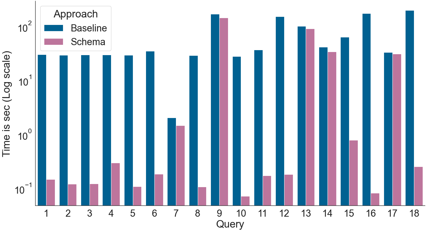
Figure 12. Query runtime for YAGO dataset.

All (third-party) queries considered in these YAGO experiments happen to be acyclic (A) recursive (RQ) graph queries. In order to further experimentally assess the impact of the approach on performance, we next investigate with graphs of different topology and varying sizes, in combination with other query shapes and types (e.g. cyclic, non-recursive).

5.4. Performance results on LDBC

We execute the 30 queries of Table 4 for the 5 different scales of the LDBC-SNB datasets, for both the schema-based approach and the baseline. Therefore each query is run $5\times 2=10$ times, which yields 300 query runs. Some queries did not execute successfully (timed out). Among the successful executions, times spent in evaluations can significantly vary from a query to another. In order to extract useful insights from these measurements, we resort to statistical measures and aggregations on successful executions, using the bootstrapping technique (Tibshirani and Efron, 1993). Specifically, we test the hypothesis that performance of query execution is improved by the schema-based approach for some query shapes or types.

We conduct this test across all scale factors. In order to have consistent measures accross the different scale factors, we retain only queries that executed successfully throughout all scale factors. This was the case for 18 queries (while 12 did timeout after a given scale factor).

We used the bootstrapping technique to generate 10,000 uniformly distributed random samples with replacement for both approaches across five scale factors. In other terms, for each scale factor, 10,000 samples with replacement are randomly picked out of the 18 pairs (query, evaluation time). Then the median, and 95% confidence intervals are computed . We show the results for the different query shapes and types for graphs of increasing sizes.

Impact of query shape.

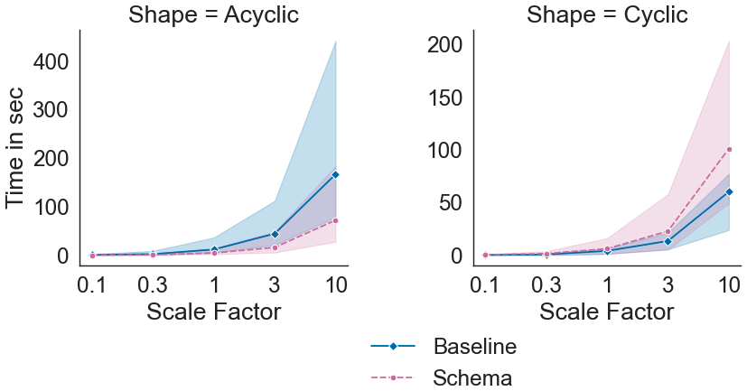
Figure 13. Runtime based on query shape.

Fig. 13 shows the median query run time of acyclic and cyclic-shaped queries for the five scale factors. This suggests that the schema-based approach is more efficient for executing acyclic queries, especially when the dataset size increases. For cyclic queries the baseline performs better. For acylic queries, the median query run times presented in Fig. 13 suggest that more acyclic queries ran faster using the schema-based approach.

Impact of recursion.

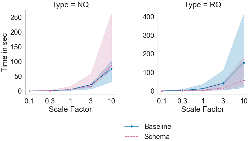
Figure 14. Runtime based on query type.

Fig. 14 presents the median query run time of recursive and non-recursive queries for the five scale factors. This suggests that the schema-based approach is more efficient for executing recursive graph queries, especially when the data set size increases. The median query run times presented in Fig. 14 suggest that more recursive graph queries ran faster using the schema-based approach.

Performance analysis when shapes are combined with recursion.

Findings in Sec. 5.3 and Sec. 5.4 suggest that the schema-based approach can significantly impact the performance of acylic queries on one side and of recursive queries on the other side, especially when dealing with large data sets.

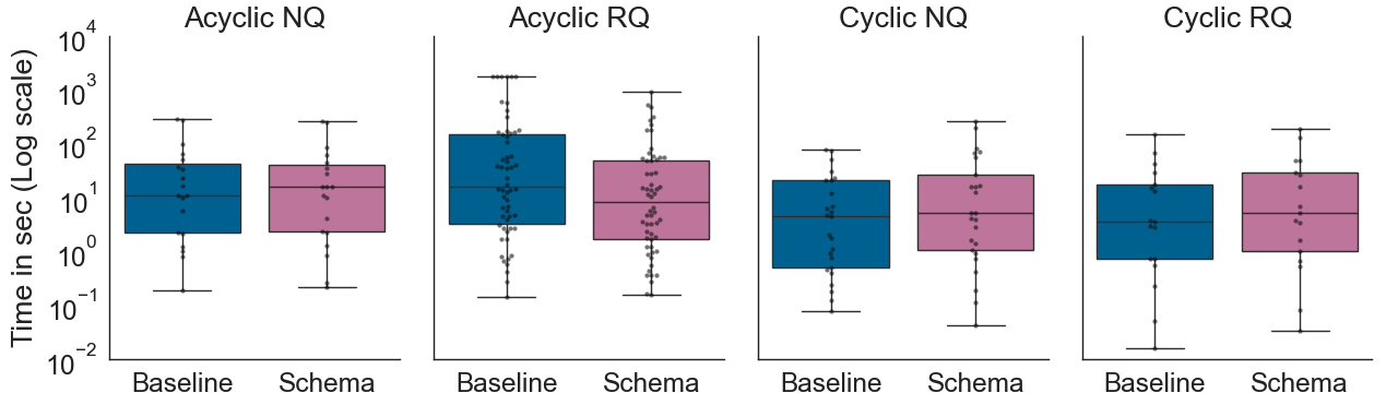
Figure 15. Query runtime summary statistics.

In order to analyze the combined effect of query shapes and types, Fig. 15 presents a summary of statistics based on box plots for all the successful runs of the 30 queries of Table 4. In these plots, queries are categorized by both shape and type, namely: acyclic recursive graph queries (Acyclic RQ), acyclic non-recursive graph queries (Acyclic NQ), cyclic recursive graph queries (Cyclic RQ), and cyclic non-recursive graph queries (Cyclic NQ). Plots use a log scale.

Furthermore, Table 6 compares schema-based (S) and baseline (non schema-based) (B) approaches in query runtime where COUNT, MIN, Q1, Q2, Q3 and MAX represent total number of queries, minimum, 25^th percentile, median, 75^th percentile and maximum query runtime (in seconds) respectively.

Table 6. Five point summary of query runtime (in seconds)

	Acyclic RQ		Acyclic NQ		Cyclic RQ		Cyclic NQ
	B	S	B	S	B	S	B	S
COUNT	58	58	19	19	17	17	25	25
MIN	0.15	0.16	0.19	0.21	0.016	0.034	0.07	0.04
Q1	3.33	1.72	2.25	2.34	0.72	1.024	0.51	1.06
Q2	16.32	8.58	11.17	16.1	3.59	5.29	4.49	5.27
Q3	155.38	50.58	44.25	40.69	17.51	29.82	21.29	26.91
MAX	1800	935.14	287	262.92	152	188.95	77.4	269.96

Results of Figure 15 and Table 6 show that for acyclic non-recursive queries, both approaches are comparable. For cyclic queries, schema based query enhancement does not seem appropriate. Intuitively, cyclic queries use the conjunction operator for additional filtering on the source and target attributes of the edge relations. As a result, for cyclic queries, the schema-based approach introduces additional semi-joins concerning node relations, which may require more processing time to filter the intermediate tuples. Overall, results show that the schema-based approach is more efficient than the baseline for acyclic recursive graph queries.

5.5. Evaluation on other RDBMS

We now test whether the previous results can also be observed on other relational database systems. To this end, we compared the results obtained on three popular open-source RDBMS: PostgreSQL, MySQL, and SQLite. We conducted experiments on LDBC-SNB and YAGO datasets focusing on acyclic-shaped recursive graph queries.

Fig. 16 displays the box plot-based summary statistics of query runtime for the schema-based approach and the baseline for the YAGO dataset. The schema-based approach consistently outperforms the baseline for all queries on the three RDBMS PostgreSQL, MySQL, and SQLite.

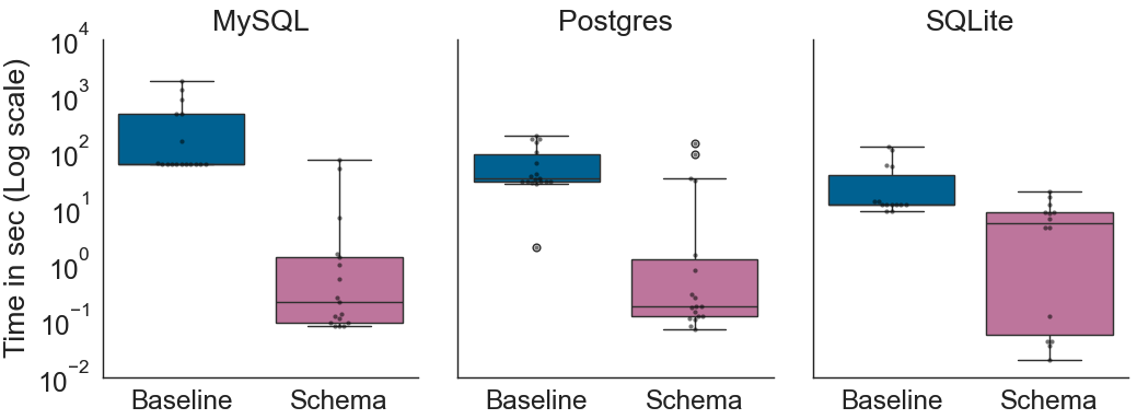
Figure 16. Query runtime on different RDBMS for YAGO.

Fig. 17 shows the box plot-based summary statistics for query runtime for the LDBC-SNB dataset for all scale factors. The schema-based approach outperforms the baseline. Notice that for scale factors 3 and 10, both MySQL and SQLite could not execute the queries within 30 minutes (the box plots use the timeout values for these cases).

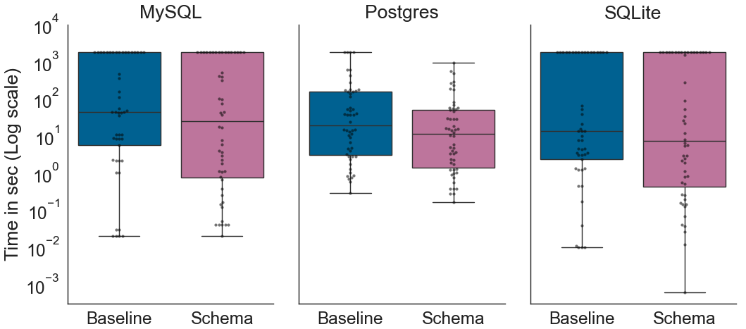
Figure 17. Query runtime on different RDBMS for LDBC.

As shown in Figures 16 and 17, the median query runtime of the schema-based approach is better than the baseline across all RDBMS. As a side remark, we observe that PostgreSQL better supports query evaluation on larger datasets.

6. Related Work

Two main approaches for logical query optimisation are (i) view-based query rewriting and (ii) schema-based query rewriting (Grahne and Thomo, 2003c; Chakravarthy et al., 1990).

6.1. View-based query rewriting

View-based query rewriting dates back to the nineties when such approaches were first studied in the context of conjunctive queries (CQ) (Chen and Roussopoulos, 1994; Yang and Larson, 1987; Sellis, 1988; Stonebraker et al., 1990). These ideas have been further explored for graph query language formalisms such as RPQ, 2RPQ and C2RPQ (Beeri et al., 1997; Halevy, 2001; Calvanese et al., 1999, 2000a, 2000b; Li et al., 2016; Adali et al., 1996; Grahne and Thomo, 2003a, b). View-based query rewriting has been proposed for XML (Fan et al., 2006; Arion et al., 2007; Manolescu et al., 2011; Wu et al., 2009; Xu and Özsoyoglu, 2005) and DATALOG (Abiteboul and Duschka, 1998; Duschka and Genesereth, 1997; Levy et al., 1995; Afrati et al., 1999) queries using materialised views. However, materialised views depend on the database instances. Therefore, queries rewritten using views must be altered when the database instance is updated or modified (Adali et al., 1996; Afrati et al., 1999).

6.2. Schema-based query rewriting

Changes to the database schema occur less frequently than changes to the database instance (Maule et al., 2008; Curino et al., 2008). Thus, query rewriting techniques that rely on the structural information of the schema have been proposed (Chakravarthy et al., 1990). Authors in (Abiteboul and Vianu, 1997; Buneman et al., 1998, 2000b; Vielle, 1989) emphasize the schema’s significance in the query rewriting. Additionally, authors in (Buneman et al., 1997; Fernandez and Suciu, 1998) suggest that knowing the structure of the database can help reduce the query search space, leading to a significant improvement in overall query runtime. We now briefly discuss schema-based query rewriting techniques proposed for databases following different data models.

6.2.1. Semi-structured databases

Schema-based query rewriting techniques for queries over semi-structured databases is proposed in (Abiteboul and Vianu, 1997; Buneman et al., 1998, 2000b). In semi-structured databases, schemas are expressed as path constraints that are regular expressions defined over edge labels (Buneman et al., 2000a). The use of path constraints to rewrite queries expressed in the formalism of C2RPQ and UC2RPQ is proposed in (Deutsch and Tannen, 2001; Calvanese et al., 1998; Florescu et al., 1998). However, a significant limitation of using path constraints as a schema language is that the schema database consistency can only be established when path constraints are defined without using the Kleene star operator (Buneman et al., 2000b).

6.2.2. XML databases

Authors in (Neven and Schwentick, 2006; Wood, 2003) propose rewriting XPath queries using the structural information stored in the schema of XML databases. For XML databases, schemas are expressed as Document Type Definition (DTDs), which are essentially regular expressions defined over the edge labels (Martens, 2022). Authors (Miklau and Suciu, 2004; Benedikt et al., 2008; Lakshmanan et al., 2004; Geerts and Fan, 2005; Hidders, 2004; Czerwiński et al., 2015) study the satisfiability of XPath queries in presence of DTDs and suggest that satisfiability is undecidable for XPath queries in presence of recursive DTDs (DTDs defined using Kleene star operator). Authors in (Bressan et al., 2005; Marian and Siméon, 2003) propose the creation of smaller XML documents by using the XPath query and structure of XML schema. Authors in (Benzaken et al., 2006) suggest a type system-based approach for XML document pruning; however, they highlight that creating pruned XML documents can be time-consuming and may take a similar amount of time as running the original query.

6.2.3. DATALOG

Schema-based query rewriting of conjunctive queries (CQ) and union of conjunctive queries (UCQ) in the presence of schema expressed as DATALOG rules is proposed in (Meier et al., 2010). Furthermore, authors (Barceló et al., 2020) suggest that query containment of CQ and UCQ is decidable in the presence of schema expressed as non-recursive DATALOG. Authors (Bancilhon et al., 1985; Vielle, 1989; de Moor et al., 2008; Schäfer and de Moor, 2010) study the containment of DATALOG queries in the presence of schema and suggest that the containment is decidable in the presence of non-recursive schemas. Regarding graph query language formalism, authors in (Bonatti, 2004; Calvanese et al., 1998; Calvanese et al., 2005) express the formalisms of C2RPQ and UC2RPQ as DATALOG queries and suggest that the query containment is decidable in the presence of non-recursive DATALOG schema.

6.2.4. Graph databases

Graph query and schema languages have been extensively researched in the context of knowledge graphs (Wiharja et al., 2020; Hu et al., 2022; Bellomarini et al., 2022) with RDFS and OWL in particular (Henriksson and Małuszyński, 2004; Lu et al., 2007), and the standard query language SPARQL (Bonifati et al., 2020b; Haller, 2023; Chekol et al., 2018, 2012). Query rewriting based on the structure of the Resource Description Framework (RDF) has been proposed in (Kim et al., 2017; Abbas et al., 2017) for non-recursive SPARQL queries.

For property graphs, significant research and standardisation effort are still in progress (Sakr et al., 2021b; Bonifati, 2021; Sakr et al., 2021a; Bonifati and Voigt, 2022; Bonifati et al., 2023a; Rost et al., 2024; Deutsch et al., 2022; Francis et al., 2023b; Angles et al., 2018). So far, the lack of standard schema language hinders the application of schema-based query rewriting techniques. Contemporary research in property graph data models mainly focuses on property graph schema design and inference techniques (Alotaibi et al., 2021; Lbath et al., 2021; Ragab, 2020; Sakr et al., 2021b; Bonifati et al., 2023b, 2022, 2019). The design of our graph schema is motivated by existing works such as PG-Schema and PG-Keys proposed in (Angles et al., 2023, 2021).

In (Colazzo and Sartiani, 2015), a type inference approach is proposed to rewrite queries expressed in the formalisms of RPQ and 2RPQ using a recursive graph schema. However, the type inference system presented in (Colazzo and Sartiani, 2015) is neither sound nor complete for graph query language formalisms containing branching and conjunction operations. Additionally, the type inference system is only explored theoretically.

Compared to the state-of-the-art, our approach can take a UCQT query and a graph schema as input and generate a UCQT query as output, which is enhanced with structural schema information. The rewritten schema-aware query preserves the initial query semantics under the graph schema. We experimentally demonstrate that for acyclic-shaped recursive UCQTs, the generated UCQT can be executed more efficiently using our approach.

7. Conclusion and Perspectives

We propose a graph query rewriting technique based on the structural information stored in a graph schema. The purpose is to enrich an initial query with schema information in order to improve query execution. To this end, we introduce inference rules capable of incorporating schema constraints in the path expressions contained in a query. The difficulty comes from the fact that pushing constraints through regular path expressions is complex. This automatizes a process which would be tricky and error-prone if done manually by a developer. Furthermore, the soundness and completeness of the approach are proved to ensure that the initial query semantics is preserved under the schema.

We conducted extensive experiments on real and synthetic datasets. We have also tested with queries of different shape and type, and on several relational database systems. Experimental results show that schema-based query rewriting provides significant performance gains for acyclic recursive graph queries.

A perspective for further work is to extend the approach by considering properties and aggregrations toward more analytical-style queries.

References

- (1)
- Abbas et al. (2017) Abdullah Abbas, Pierre Genevès, Cécile Roisin, and Nabil Layaïda. 2017. Optimising SPARQL query evaluation in the presence of shex constraints. In BDA 2017-33ème conférence sur la \guillemotleftGestion de Données—Principes, Technologies et Applications\guillemotright. 1–12.
- Abiteboul and Duschka (1998) Serge Abiteboul and Oliver M Duschka. 1998. Complexity of answering queries using materialized views. In Proceedings of the seventeenth ACM SIGACT-SIGMOD-SIGART symposium on Principles of database systems. 254–263.
- Abiteboul and Vianu (1997) Serge Abiteboul and Victor Vianu. 1997. Regular path queries with constraints. In Proceedings of the sixteenth ACM SIGACT-SIGMOD-SIGART symposium on Principles of database systems. 122–133.
- Abul-Basher et al. (2017) Zahid Abul-Basher, Nikolay Yakovets, Parke Godfrey, Shadi Ghajar-Khosravi, and Mark H Chignell. 2017. Tasweet: optimizing disjunctive regular path queries in graph databases. In EDBT/ICDT 2017 Joint Conference 20th International Conference on Extending Database Technology. 470–473.
- Adali et al. (1996) Sibel Adali, K Selçuk Candan, Yannis Papakonstantinou, and Vo S Subrahmanian. 1996. Query caching and optimization in distributed mediator systems. ACM SIGMOD Record 25, 2 (1996), 137–146.
- Afrati et al. (1999) Foto N Afrati, Manolis Gergatsoulis, and Theodoros Kavalieros. 1999. Answering queries using materialized views with disjunctions. In Database Theory—ICDT’99: 7th International Conference Jerusalem, Israel, January 10–12, 1999 Proceedings 7. Springer, 435–452.
- Agrawal (1988) Rakesh Agrawal. 1988. Alpha: An extension of relational algebra to express a class of recursive queries. IEEE Transactions on Software Engineering 14, 7 (1988), 879–885.
- Alotaibi et al. (2021) Rana Alotaibi, Chuan Lei, Abdul Quamar, Vasilis Efthymiou, and Fatma Özcan. 2021. Property graph schema optimization for domain-specific knowledge graphs. In 2021 IEEE 37th International Conference on Data Engineering (ICDE). IEEE, 924–935.
- Angles et al. (2018) Renzo Angles, Marcelo Arenas, Pablo Barceló, Peter Boncz, George Fletcher, Claudio Gutierrez, Tobias Lindaaker, Marcus Paradies, Stefan Plantikow, Juan Sequeda, et al. 2018. G-CORE: A core for future graph query languages. In Proceedings of the 2018 International Conference on Management of Data. 1421–1432.
- Angles et al. (2017) Renzo Angles, Marcelo Arenas, Pablo Barceló, Aidan Hogan, Juan Reutter, and Domagoj Vrgoč. 2017. Foundations of modern query languages for graph databases. ACM Computing Surveys (CSUR) 50, 5 (2017), 1–40.
- Angles et al. (2023) Renzo Angles, Angela Bonifati, Stefania Dumbrava, George Fletcher, Alastair Green, Jan Hidders, Bei Li, Leonid Libkin, Victor Marsault, Wim Martens, et al. 2023. PG-Schema: Schemas for property graphs. Proceedings of the ACM on Management of Data 1, 2 (2023), 1–25.
- Angles et al. (2021) Renzo Angles, Angela Bonifati, Stefania Dumbrava, George Fletcher, Keith W Hare, Jan Hidders, Victor E Lee, Bei Li, Leonid Libkin, Wim Martens, et al. 2021. Pg-keys: Keys for property graphs. In Proceedings of the 2021 International Conference on Management of Data. 2423–2436.
- Angles et al. (2020) Renzo Angles, Harsh Thakkar, and Dominik Tomaszuk. 2020. Mapping RDF databases to property graph databases. IEEE Access 8 (2020), 86091–86110.
- Aref et al. (2015) Molham Aref, Balder ten Cate, Todd J Green, Benny Kimelfeld, Dan Olteanu, Emir Pasalic, Todd L Veldhuizen, and Geoffrey Washburn. 2015. Design and implementation of the LogicBlox system. In Proceedings of the 2015 ACM SIGMOD International Conference on Management of Data. 1371–1382.
- Arion et al. (2007) Andrei Arion, Véronique Benzaken, Ioana Manolescu, and Yannis Papakonstantinou. 2007. Structured materialized views for XML queries. In Proceedings of the 33rd international conference on Very large data bases. 87–98.
- Bancilhon et al. (1985) Francois Bancilhon, David Maier, Yehoshua Sagiv, and Jeffrey D Ullman. 1985. Magic sets and other strange ways to implement logic programs. In Proceedings of the fifth ACM SIGACT-SIGMOD symposium on Principles of database systems. 1–15.
- Barceló et al. (2020) Pablo Barceló, Diego Figueira, Georg Gottlob, and Andreas Pieris. 2020. Semantic optimization of conjunctive queries. Journal of the ACM (JACM) 67, 6 (2020), 1–60.
- Barceló et al. (2013) Pablo Barceló, Jorge Pérez, and Juan Reutter. 2013. Schema mappings and data exchange for graph databases. In Proceedings of the 16th International Conference on Database Theory. 189–200.
- Barrett et al. (2000) Chris Barrett, Riko Jacob, and Madhav Marathe. 2000. Formal-language-constrained path problems. SIAM J. Comput. 30, 3 (2000), 809–837.
- Beeri et al. (1997) Catriel Beeri, Alon Y Levy, and Marie-Christine Rousset. 1997. Rewriting queries using views in description logics. In Proceedings of the sixteenth ACM SIGACT-SIGMOD-SIGART symposium on Principles of database systems. 99–108.
- Bell et al. (2009) Gordon Bell, Tony Hey, and Alex Szalay. 2009. Beyond the data deluge. Science 323, 5919 (2009), 1297–1298.
- Bellomarini et al. (2022) Luigi Bellomarini, Andrea Gentili, Eleonora Laurenza, and Emanuel Sallinger. 2022. Model-Independent Design of Knowledge Graphs-Lessons Learnt From Complex Financial Graphs.. In EDBT. 2–524.
- Benedikt et al. (2008) Michael Benedikt, Wenfei Fan, and Floris Geerts. 2008. XPath satisfiability in the presence of DTDs. Journal of the ACM (JACM) 55, 2 (2008), 1–79.
- Benzaken et al. (2006) Véronique Benzaken, Giuseppe Castagna, Dario Colazzo, and Kim Nguyen. 2006. Type-Based XML Projection.. In VLDB, Vol. 6. 271–282.
- Bonatti (2004) Piero A Bonatti. 2004. On the decidability of containment of recursive datalog queries-preliminary report. In Proceedings of the twenty-third ACM SIGMOD-SIGACT-SIGART symposium on Principles of database systems. 297–306.
- Bonifati (2021) Angela Bonifati. 2021. Graph processing systems back to the future. In Proceedings of the 4th ACM SIGMOD Joint International Workshop on Graph Data Management Experiences & Systems (GRADES) and Network Data Analytics (NDA). 1–1.
- Bonifati et al. (2023a) Angela Bonifati, Stefania Dumbrava, George Fletcher, Jan Hidders, Matthias Hofer, Wim Martens, Filip Murlak, Joshua Shinavier, Slawek Staworko, and Dominik Tomaszuk. 2023a. Threshold Queries. ACM SIGMOD Record 52, 1 (2023), 64–73.
- Bonifati et al. (2022) Angela Bonifati, Stefania Dumbrava, Emile Martinez, Fatemeh Ghasemi, Malo Jaffré, Pacôme Luton, and Thomas Pickles. 2022. DiscoPG: property graph schema discovery and exploration. Proceedings of the VLDB Endowment 15, 12 (2022), 3654–3657.
- Bonifati et al. (2023b) Angela Bonifati, Stefania Dumbrava, Emile Martinez, and Nicolas Mir. 2023b. The Quest for Schemas in Graph Databases. Looking Ahead 4 (2023), 5.
- Bonifati et al. (2018) Angela Bonifati, George Fletcher, Hannes Voigt, Nikolay Yakovets, and HV Jagadish. 2018. Querying graphs. Vol. 10. Springer.
- Bonifati et al. (2019) Angela Bonifati, Peter Furniss, Alastair Green, Russ Harmer, Eugenia Oshurko, and Hannes Voigt. 2019. Schema validation and evolution for graph databases. In Conceptual Modeling: 38th International Conference, ER 2019, Salvador, Brazil, November 4–7, 2019, Proceedings 38. Springer, 448–456.
- Bonifati et al. (2020a) Angela Bonifati, Wim Martens, and Thomas Timm. 2020a. An analytical study of large SPARQL query logs. The VLDB Journal 29, 2-3 (2020), 655–679.
- Bonifati et al. (2020b) Angela Bonifati, Wim Martens, and Thomas Timm. 2020b. SHARQL: Shape analysis of recursive SPARQL queries. In Proceedings of the 2020 ACM SIGMOD International Conference on Management of Data. 2701–2704.
- Bonifati and Voigt (2022) Angela Bonifati and Hannes Voigt. 2022. Special issue on big graph data management and processing. The VLDB Journal 31, 2 (2022), 201–202.
- Bornea et al. (2013) Mihaela A Bornea, Julian Dolby, Anastasios Kementsietsidis, Kavitha Srinivas, Patrick Dantressangle, Octavian Udrea, and Bishwaranjan Bhattacharjee. 2013. Building an efficient RDF store over a relational database. In Proceedings of the 2013 ACM SIGMOD International Conference on Management of Data. 121–132.
- Bressan et al. (2005) Stéphane Bressan, Barbara Catania, Zoé Lacroix, Ying Guang Li, and Anna Maddalena. 2005. Accelerating queries by pruning XML documents. Data & Knowledge Engineering 54, 2 (2005), 211–240.
- Buneman et al. (1997) Peter Buneman, Susan Davidson, Mary Fernandez, and Dan Suciu. 1997. Adding structure to unstructured data. In Database Theory—ICDT’97: 6th International Conference Delphi, Greece, January 8–10, 1997 Proceedings 6. Springer, 336–350.
- Buneman et al. (1998) Peter Buneman, Wenfei Fan, and Scott Weinstein. 1998. Path constraints on semistructured and structured data. In Proceedings of the seventeenth ACM SIGACT-SIGMOD-SIGART symposium on Principles of database systems. 129–138.
- Buneman et al. (2000a) Peter Buneman, Wenfei Fan, and Scott Weinstein. 2000a. Path constraints in semistructured databases. J. Comput. System Sci. 61, 2 (2000), 146–193.
- Buneman et al. (2000b) Peter Buneman, Wenfei Fan, and Scott Weinstein. 2000b. Query optimization for semistructured data using path constraints in a deterministic data model. In Research Issues in Structured and Semistructured Database Programming: 7th International Workshop on Database Programming Languages, DBPL’99 Kinloch Rannoch, UK, September 1–3, 1999 Revised Papers 7. Springer, 208–223.
- Calvanese et al. (1998) Diego Calvanese, Giuseppe De Giacomo, and Maurizio Lenzerini. 1998. On the decidability of query containment under constraints. In Proceedings of the seventeenth ACM SIGACT-SIGMOD-SIGART symposium on Principles of database systems. 149–158.
- Calvanese et al. (1999) Diego Calvanese, Giuseppe De Giacomo, Maurizio Lenzerini, and Moshe Y Vardi. 1999. Rewriting of regular expressions and regular path queries. In Proceedings of the eighteenth ACM SIGMOD-SIGACT-SIGART symposium on Principles of database systems. 194–204.
- Calvanese et al. (2000a) Diego Calvanese, Giuseppe De Giacomo, Maurizio Lenzerini, and Moshe Y Vardi. 2000a. Answering regular path queries using views. In Proceedings of 16th International Conference on Data Engineering (Cat. No. 00CB37073). IEEE, 389–398.
- Calvanese et al. (2005) Diego Calvanese, Giuseppe De Giacomo, and Moshe Y Vardi. 2005. Decidable containment of recursive queries. Theoretical Computer Science 336, 1 (2005), 33–56.
- Calvanese et al. (2000b) Diego Calvanese, Moshe Y Vardi, Giuseppe de Giacomo, and Maurizio Lenzerini. 2000b. View-based query processing for regular path queries with inverse. In Proceedings of the nineteenth ACM SIGMOD-SIGACT-SIGART symposium on Principles of database systems. 58–66.
- Chakravarthy et al. (1990) Upen S Chakravarthy, John Grant, and Jack Minker. 1990. Logic-based approach to semantic query optimization. ACM Transactions on Database Systems (TODS) 15, 2 (1990), 162–207.
- Chekol et al. (2012) Melisachew Wudage Chekol, Jérôme Euzenat, Pierre Genevès, and Nabil Layaïda. 2012. SPARQL query containment under SHI axioms. In Proceedings of the AAAI Conference on Artificial Intelligence, Vol. 26. 10–16.
- Chekol et al. (2018) Melisachew Wudage Chekol, Jérôme Euzenat, Pierre Genevès, and Nabil Layaïda. 2018. SPARQL query containment under schema. Journal on Data Semantics 7, 3 (2018), 133–154.
- Chen and Roussopoulos (1994) Chungmin Melvin Chen and Nicholas Roussopoulos. 1994. The implementation and performance evaluation of the ADMS query optimizer: Integrating query result caching and matching. In International Conference on Extending Database Technology. Springer, 323–336.
- Colazzo and Sartiani (2015) Dario Colazzo and Carlo Sartiani. 2015. Typing regular path query languages for data graphs. In Proceedings of the 15th Symposium on Database Programming Languages. 69–78.
- Curino et al. (2008) Carlo A Curino, Hyun J Moon, and Carlo Zaniolo. 2008. Graceful database schema evolution: the prism workbench. Proceedings of the VLDB Endowment 1, 1 (2008), 761–772.
- Czerwiński et al. (2015) Wojciech Czerwiński, Wim Martens, Pawel Parys, and Marcin Przybylko. 2015. The (almost) complete guide to tree pattern containment. In Proceedings of the 34th ACM SIGMOD-SIGACT-SIGAI Symposium on Principles of Database Systems. 117–130.
- de Moor et al. (2008) Oege de Moor, Damien Sereni, Pavel Avgustinov, and Mathieu Verbaere. 2008. Type inference for datalog and its application to query optimisation. In Proceedings of the twenty-seventh ACM SIGMOD-SIGACT-SIGART symposium on Principles of database systems. 291–300.
- Deutsch et al. (2022) Alin Deutsch, Nadime Francis, Alastair Green, Keith Hare, Bei Li, Leonid Libkin, Tobias Lindaaker, Victor Marsault, Wim Martens, Jan Michels, et al. 2022. Graph pattern matching in GQL and SQL/PGQ. In Proceedings of the 2022 International Conference on Management of Data. 2246–2258.
- Deutsch and Tannen (2001) Alin Deutsch and Val Tannen. 2001. Optimization properties for classes of conjunctive regular path queries. In International Workshop on Database Programming Languages. Springer, 21–39.
- Duschka and Genesereth (1997) Oliver M Duschka and Michael R Genesereth. 1997. Answering recursive queries using views. In Proceedings of the sixteenth ACM SIGACT-SIGMOD-SIGART symposium on Principles of database systems. 109–116.
- Duschka et al. (2000) Oliver M Duschka, Michael R Genesereth, and Alon Y Levy. 2000. Recursive query plans for data integration. The Journal of Logic Programming 43, 1 (2000), 49–73.
- Erling et al. (2015) Orri Erling, Alex Averbuch, Josep Larriba-Pey, Hassan Chafi, Andrey Gubichev, Arnau Prat, Minh-Duc Pham, and Peter Boncz. 2015. The LDBC social network benchmark: Interactive workload. In Proceedings of the 2015 ACM SIGMOD International Conference on Management of Data. 619–630.
- Fan et al. (2006) Wenfei Fan, Floris Geerts, Xibei Jia, and Anastasios Kementsietsidis. 2006. Rewriting regular XPath queries on XML views. In 2007 IEEE 23rd International Conference on Data Engineering. IEEE, 666–675.
- Fejza et al. (2023) Amela Fejza, Pierre Genevès, Nabil Layaïda, and Sarah Chlyah. 2023. The -RA System for Recursive Path Queries over Graphs. In Proceedings of the 32nd ACM International Conference on Information and Knowledge Management. 5041–5045.
- Fernandez and Suciu (1998) Mary Fernandez and Dan Suciu. 1998. Optimizing regular path expressions using graph schemas. In Proceedings 14th International Conference on Data Engineering. IEEE, 14–23.
- Florescu et al. (1998) Daniela Florescu, Alon Levy, and Dan Suciu. 1998. Query containment for conjunctive queries with regular expressions. In Proceedings of the seventeenth ACM SIGACT-SIGMOD-SIGART symposium on Principles of database systems. 139–148.
- Francis et al. (2023a) Nadime Francis, Amélie Gheerbrant, Paolo Guagliardo, Leonid Libkin, Victor Marsault, Wim Martens, Filip Murlak, Liat Peterfreund, Alexandra Rogova, and Domagoj Vrgoc. 2023a. GPC: A pattern calculus for property graphs. In Proceedings of the 42nd ACM SIGMOD-SIGACT-SIGAI Symposium on Principles of Database Systems. 241–250.
- Francis et al. (2023b) Nadime Francis, Amélie Gheerbrant, Paolo Guagliardo, Leonid Libkin, Victor Marsault, Wim Martens, Filip Murlak, Liat Peterfreund, Alexandra Rogova, and Domagoj Vrgoc. 2023b. A Researchers Digest of GQL. In The 26th International Conference on Database Theory, 2023. Schloss Dagstuhl-Leibniz-Zentrum für Informatik, 1–1.
- Francis et al. (2018) Nadime Francis, Alastair Green, Paolo Guagliardo, Leonid Libkin, Tobias Lindaaker, Victor Marsault, Stefan Plantikow, Mats Rydberg, Petra Selmer, and Andrés Taylor. 2018. Cypher: An evolving query language for property graphs. In Proceedings of the 2018 international conference on management of data. 1433–1445.
- Geerts and Fan (2005) Floris Geerts and Wenfei Fan. 2005. Satisfiability of XPath queries with sibling axes. In International Workshop on Database Programming Languages. Springer, 122–137.
- Genevès and Layaïda (2006) Pierre Genevès and Nabil Layaïda. 2006. A system for the static analysis of XPath. ACM Trans. Inf. Syst. 24, 4 (2006), 475–502. https://doi.org/10.1145/1185877.1185882
- Gomes-Jr et al. (2015) Luiz Gomes-Jr, Bernd Amann, and André Santanchè. 2015. Beta-algebra: Towards a relational algebra for graph analysis. In EDBT/ICDT 2015 Joint Conference, Vol. 157.
- Grahne and Thomo (2003a) Gösta Grahne and Alex Thomo. 2003a. Algebraic rewritings for optimizing regular path queries. Theoretical Computer Science 296, 3 (2003), 453–471.
- Grahne and Thomo (2003b) Gösta Grahne and Alex Thomo. 2003b. New rewritings and optimizations for regular path queries. In Database Theory—ICDT 2003: 9th International Conference Siena, Italy, January 8–10, 2003 Proceedings 9. Springer, 242–258.
- Grahne and Thomo (2003c) Gösta Grahne and Alex Thomo. 2003c. Query containment and rewriting using views for regular path queries under constraints. In Proceedings of the twenty-second ACM SIGMOD-SIGACT-SIGART symposium on Principles of database systems. 111–122.
- Gubichev et al. (2013) Andrey Gubichev, Srikanta J Bedathur, and Stephan Seufert. 2013. Sparqling kleene: fast property paths in RDF-3X. In First International Workshop on Graph Data Management Experiences and Systems. 1–7.
- Halevy (2001) Alon Y Halevy. 2001. Answering queries using views: A survey. The VLDB Journal 10 (2001), 270–294.
- Haller (2023) David Haller. 2023. A Query-Driven Approach for SHACL Type Inference. In Conference on Very Large Data Bases (VLDB 2023).
- Hellings (2018) Jelle Hellings. 2018. On Tarski’s Relation Algebra: querying trees and chains and the semi-join algebra.
- Hellings et al. (2023) Jelle Hellings, Marc Gyssens, Jan Van Den Bussche, and Dirk Van Gucht. 2023. Expressive Completeness of Two-Variable First-Order Logic with Counting for First-Order Logic Queries on Rooted Unranked Trees. In 2023 38th Annual ACM/IEEE Symposium on Logic in Computer Science (LICS). IEEE, 1–13.
- Hellings et al. (2020) Jelle Hellings, Marc Gyssens, Yuqing Wu, Dirk Van Gucht, Jan Van den Bussche, Stijn Vansummeren, and George HL Fletcher. 2020. Comparing the expressiveness of downward fragments of the relation algebra with transitive closure on trees. Information Systems 89 (2020), 101467.
- Hellings et al. (2017) Jelle Hellings, Catherine L Pilachowski, Dirk Van Gucht, Marc Gyssens, and Yuqing Wu. 2017. From relation algebra to semi-join algebra: An approach for graph query optimization. In Proceedings of the 16th International Symposium on Database Programming Languages. 1–10.
- Henriksson and Małuszyński (2004) Jakob Henriksson and Jan Małuszyński. 2004. Static type-checking of Datalog with ontologies. In Principles and Practice of Semantic Web Reasoning: Second International Workshop, PPSWR 2004, St. Malo, France, September 6-10, 2004. Proceedings 2. Springer, 76–89.
- Hidders (2004) Jan Hidders. 2004. Satisfiability of XPath expressions. In Database Programming Languages: 9th International Workshop, DBPL 2003, Potsdam, Germany, September 6-8, 2003. Revised Papers 9. Springer, 21–36.
- Hoffart et al. (2013) Johannes Hoffart, Fabian M. Suchanek, Klaus Berberich, and Gerhard Weikum. 2013. YAGO2: A spatially and temporally enhanced knowledge base from Wikipedia. Artif. Intell. 194 (2013), 28–61. https://doi.org/10.1016/J.ARTINT.2012.06.001
- Hogan and Hogan (2020) Aidan Hogan and Aidan Hogan. 2020. SPARQL query language. The Web of Data (2020), 323–448.
- Hu et al. (2022) Zhiwei Hu, Víctor Gutiérrez-Basulto, Zhiliang Xiang, Xiaoli Li, Ru Li, and Jeff Z Pan. 2022. Type-aware embeddings for multi-hop reasoning over knowledge graphs. arXiv preprint arXiv:2205.00782 (2022).
- Jaakkola and Kuusisto (2023) Reijo Jaakkola and Antti Kuusisto. 2023. Complexity Classifications via Algebraic Logic. In 31st EACSL Annual Conference on Computer Science Logic, CSL 2023. Schloss Dagstuhl-Leibniz-Zentrum für Informatik.
- Jachiet et al. (2020) Louis Jachiet, Pierre Genevès, Nils Gesbert, and Nabil Layaïda. 2020. On the optimization of recursive relational queries: Application to graph queries. In Proceedings of the 2020 ACM SIGMOD International Conference on Management of Data. 681–697.
- Jindal et al. (2014) Alekh Jindal, Praynaa Rawlani, Eugene Wu, Samuel Madden, Amol Deshpande, and Mike Stonebraker. 2014. Vertexica: your relational friend for graph analytics! (2014).
- Kim et al. (2017) HyeongSik Kim, Padmashree Ravindra, and Kemafor Anyanwu. 2017. Type-based semantic optimization for scalable RDF graph pattern matching. In Proceedings of the 26th International Conference on World Wide Web. 785–793.
- Lakshmanan et al. (2004) Laks VS Lakshmanan, Ganesh Ramesh, Hui Wang, and Zheng Zhao. 2004. On testing satisfiability of tree pattern queries. In VLDB, Vol. 4. 120–131.
- Lbath et al. (2021) Hanâ Lbath, Angela Bonifati, and Russ Harmer. 2021. Schema inference for property graphs. In EDBT 2021-24th International Conference on Extending Database Technology. 499–504.
- Leeuwen et al. (2022) Wilco v Leeuwen, Thomas Mulder, Bram van de Wall, George Fletcher, and Nikolay Yakovets. 2022. Avantgraph query processing engine. Proceedings of the VLDB Endowment 15, 12 (2022), 3698–3701.
- Leone et al. (2006) Nicola Leone, Gerald Pfeifer, Wolfgang Faber, Thomas Eiter, Georg Gottlob, Simona Perri, and Francesco Scarcello. 2006. The DLV system for knowledge representation and reasoning. ACM Transactions on Computational Logic (TOCL) 7, 3 (2006), 499–562.
- Levy et al. (1995) Alon Y Levy, Alberto O Mendelzon, and Yehoshua Sagiv. 1995. Answering queries using views. In Proceedings of the fourteenth ACM SIGACT-SIGMOD-SIGART symposium on Principles of database systems. 95–104.
- Li et al. (2016) Jia Li, Yang Cao, and Xudong Liu. 2016. Approximating graph pattern queries using views. In Proceedings of the 25th ACM International on Conference on Information and Knowledge Management. 449–458.
- Libkin et al. (2013) Leonid Libkin, Wim Martens, and Domagoj Vrgoč. 2013. Querying graph databases with XPath. In Proceedings of the 16th International Conference on Database Theory. 129–140.
- Libkin et al. (2018) Leonid Libkin, Juan L Reutter, Adrián Soto, and Domagoj Vrgoč. 2018. TriAL: A navigational algebra for RDF triplestores. ACM Transactions on Database Systems (TODS) 43, 1 (2018), 1–46.
- Lu et al. (2007) Jing Lu, Li Ma, Lei Zhang, Jean-Sébastien Brunner, Chen Wang, Yue Pan, and Yong Yu. 2007. SOR: A Practical System for Ontology Storage, Reasoning and Search.. In VLDB, Vol. 7. 1402–1405.
- Manolescu et al. (2011) Ioana Manolescu, Konstantinos Karanasos, Vasilis Vassalos, and Spyros Zoupanos. 2011. Efficient XQuery rewriting using multiple views. In 2011 IEEE 27th International Conference on Data Engineering. IEEE, 972–983.
- Marian and Siméon (2003) Amélie Marian and Jérôme Siméon. 2003. Projecting XML documents. In Proceedings 2003 VLDB Conference. Elsevier, 213–224.
- Martens (2022) Wim Martens. 2022. Towards theory for real-world data. In Proceedings of the 41st ACM SIGMOD-SIGACT-SIGAI Symposium on Principles of Database Systems. 261–276.
- Maule et al. (2008) Andy Maule, Wolfgang Emmerich, and David S Rosenblum. 2008. Impact analysis of database schema changes. In Proceedings of the 30th international conference on Software engineering. 451–460.
- Meier et al. (2010) Michael Meier, Michael Schmidt, Fang Wei, and Georg Lausen. 2010. Semantic query optimization in the presence of types. In Proceedings of the twenty-ninth ACM SIGMOD-SIGACT-SIGART symposium on Principles of database systems. 111–122.
- Meimaris et al. (2017) Marios Meimaris, George Papastefanatos, Nikos Mamoulis, and Ioannis Anagnostopoulos. 2017. Extended characteristic sets: graph indexing for SPARQL query optimization. In 2017 IEEE 33rd International Conference on Data Engineering (ICDE). IEEE, 497–508.
- Mhedhbi et al. (2021) Amine Mhedhbi, Matteo Lissandrini, Laurens Kuiper, Jack Waudby, and Gábor Szárnyas. 2021. LSQB: a large-scale subgraph query benchmark. In Proceedings of the 4th ACM SIGMOD Joint International Workshop on Graph Data Management Experiences & Systems (GRADES) and Network Data Analytics (NDA). 1–11.
- Miklau and Suciu (2004) Gerome Miklau and Dan Suciu. 2004. Containment and equivalence for a fragment of XPath. Journal of the ACM (JACM) 51, 1 (2004), 2–45.
- Neumann and Moerkotte (2011) Thomas Neumann and Guido Moerkotte. 2011. Characteristic sets: Accurate cardinality estimation for RDF queries with multiple joins. In 2011 IEEE 27th International Conference on Data Engineering. IEEE, 984–994.
- Neven and Schwentick (2006) Frank Neven and Thomas Schwentick. 2006. On the complexity of XPath containment in the presence of disjunction, DTDs, and variables. Logical Methods in Computer Science 2 (2006).
- Nguyen and Kim (2017) Van-Quyet Nguyen and Kyungbaek Kim. 2017. Estimating the evaluation cost of regular path queries on large graphs. In Proceedings of the 8th International Symposium on Information and Communication Technology. 92–99.
- Pérez et al. (2006) Jorge Pérez, Marcelo Arenas, and Claudio Gutierrez. 2006. Semantics and Complexity of SPARQL. In International semantic web conference. Springer, 30–43.
- Ragab (2020) Mohamed Ragab. 2020. Large Scale Querying and Processing for Property Graphs PhD Symposium. (2020).
- Rost et al. (2024) Christopher Rost, Riccardo Tommasini, Angela Bonifati, Emanuele Della Valle, Erhard Rahm, Keith W Hare, Stefan Plantikow, Petra Selmer, and Hannes Voigt. 2024. Seraph: Continuous Queries on Property Graph Streams. (2024).
- Sakr et al. (2021a) Sherif Sakr, Angela Bonifati, Hannes Voigt, and Alexandru Iosup. 2021a. Ensuring the success of big graph processing for the next decade and beyond. Commun. ACM 64, 9 (2021).
- Sakr et al. (2021b) Sherif Sakr, Angela Bonifati, Hannes Voigt, Alexandru Iosup, Khaled Ammar, Renzo Angles, Walid Aref, Marcelo Arenas, Maciej Besta, Peter A Boncz, et al. 2021b. The future is big graphs: a community view on graph processing systems. Commun. ACM 64, 9 (2021), 62–71.
- Santana and dos Santos Mello (2019) Luiz Henrique Zambom Santana and Ronaldo dos Santos Mello. 2019. Querying in a workload-aware triplestore based on nosql databases. In Database and Expert Systems Applications: 30th International Conference, DEXA 2019, Linz, Austria, August 26–29, 2019, Proceedings, Part II 30. Springer, 159–173.
- Schäfer and de Moor (2010) Max Schäfer and Oege de Moor. 2010. Type inference for datalog with complex type hierarchies. In Proceedings of the 37th annual ACM SIGPLAN-SIGACT symposium on Principles of programming languages. 145–156.
- Sellis (1988) Timos K Sellis. 1988. Intelligent caching and indexing techniques for relational database systems. Information Systems 13, 2 (1988), 175–185.
- Shanmugasundaram et al. (1999) J Shanmugasundaram, K Tufte, C Zhang, G He, DJ DeWitt, and JF Naughton. 1999. Relational Databases for Querying XML Documents: Limitations and Opportunities, in ‘VLDB’99: Proc. of the 25th Int. Conf. on Very Large Data Bases’.
- Sharma and Sinha (2022) Chandan Sharma and Roopak Sinha. 2022. FLASc: a formal algebra for labeled property graph schema. Automated Software Engineering 29, 1 (2022), 37.
- Sharma et al. (2021) Chandan Sharma, Roopak Sinha, and Kenneth Johnson. 2021. Practical and comprehensive formalisms for modelling contemporary graph query languages. Information Systems 102 (2021), 101816.
- Sheth et al. (2005) Amit Sheth, Boanerges Aleman-Meza, I Budak Arpinar, Clemens Bertram, Yashodhan Warke, Cartic Ramakrishanan, Chris Halaschek, Kemafar Anyanwu, David Avant, F Sena Arpinar, et al. 2005. Semantic association identification and knowledge discovery for national security applications. Journal of Database Management (JDM) 16, 1 (2005), 33–53.
- Stonebraker et al. (1990) Michael Stonebraker, Anant Jhingran, Jeffrey Goh, and Spyros Potamianos. 1990. On rules, procedure, caching and views in data base systems. ACM SIGMOD Record 19, 2 (1990), 281–290.
- Suchanek et al. (2023) Fabian Suchanek, Mehwish Alam, Thomas Bonald, Pierre-Henri Paris, and Jules Soria. 2023. Integrating the Wikidata Taxonomy into YAGO. arXiv:2308.11884 [cs.AI]
- Sun et al. (2015) Wen Sun, Achille Fokoue, Kavitha Srinivas, Anastasios Kementsietsidis, Gang Hu, and Guotong Xie. 2015. Sqlgraph: An efficient relational-based property graph store. In Proceedings of the 2015 ACM SIGMOD International Conference on Management of Data. 1887–1901.
- Szárnyas (2023) Gábor Szárnyas. 2023. LDBC Social Network Benchmark graphs. https://hdl.handle.net/11112/e6e00558-a2c3-9214-473e-04a16de09bf8. https://doi.org/10.25606/SURF.8f3ac424d6694282
- Tibshirani and Efron (1993) Robert J Tibshirani and Bradley Efron. 1993. An introduction to the bootstrap. Monographs on statistics and applied probability 57, 1 (1993).
- Urbani et al. (2016) Jacopo Urbani, Ceriel JH Jacobs, and Markus Krötzsch. 2016. VLog: A Column-Oriented Datalog System for Large Knowledge Graphs.. In ISWC (Posters & Demos).
- van Rest et al. (2016) Oskar van Rest, Sungpack Hong, Jinha Kim, Xuming Meng, and Hassan Chafi. 2016. PGQL: a property graph query language. In Proceedings of the Fourth International Workshop on Graph Data Management Experiences and Systems. 1–6.
- Vielle (1989) Laurent Vielle. 1989. Recursive query processing: The power of logic. Theoretical computer science 69, 1 (1989), 1–53.
- Vrgoc (2014) Domagoj Vrgoc. 2014. Querying graphs with data. (2014).
- Wiharja et al. (2020) Kemas Wiharja, Jeff Z Pan, Martin J Kollingbaum, and Yu Deng. 2020. Schema aware iterative Knowledge Graph completion. Journal of Web Semantics 65 (2020), 100616.
- Wood (2003) Peter T Wood. 2003. Containment for XPath fragments under DTD constraints. In Database Theory—ICDT 2003: 9th International Conference Siena, Italy, January 8–10, 2003 Proceedings 9. Springer, 300–314.
- Wu et al. (2009) Xiaoying Wu, Dimitri Theodoratos, and Wendy Hui Wang. 2009. Answering XML queries using materialized views revisited. In Proceedings of the 18th ACM conference on Information and knowledge management. 475–484.
- Xirogiannopoulos et al. (2017) Konstantinos Xirogiannopoulos, Virinchi Srinivas, and Amol Deshpande. 2017. Graphgen: Adaptive graph processing using relational databases. In Proceedings of the Fifth International Workshop on Graph Data-management Experiences & Systems. 1–7.
- Xu and Özsoyoglu (2005) Wanhong Xu and Z Meral Özsoyoglu. 2005. Rewriting XPath queries using materialized views. In Proceedings of the 31st International Conference on Very Large Databases (VLDB). 121–132.
- Yago (2019) YAGO Yago. 2019. A high-quality knowledge base. https://www.mpi-inf.mpg.de/departments/databases-and-information-systems/research/yago-naga/yago.
- Yakovets et al. (2015) Nikolay Yakovets, Parke Godfrey, and Jarek Gryz. 2015. WAVEGUIDE: Evaluating SPARQL Property Path Queries.. In EDBT, Vol. 2015. 525–528.
- Yang et al. (2020) Fang Yang, Kunjie Fan, Dandan Song, and Huakang Lin. 2020. Graph-based prediction of protein-protein interactions with attributed signed graph embedding. BMC bioinformatics 21, 1 (2020), 1–16.
- Yang and Larson (1987) HZ Yang and Per-Åke Larson. 1987. Query Transformation for PSJ-Queries.. In VLDB, Vol. 87. 245–254.