Part I

Tong Zheng^1,2    Shusaku Sone¹    Yoshitaka Ushiku¹    Yuki Oba^1,3    Jiaxin Ma^{1 1}OMRON SINIC X Corporation
²Nagoya University
³Tsukuba University

TNF: Tri-branch Neural Fusion for Multimodal Medical Data Classification

Tong Zheng^1,2    Shusaku Sone¹    Yoshitaka Ushiku¹    Yuki Oba^1,3    Jiaxin Ma^{1 1}OMRON SINIC X Corporation
²Nagoya University
³Tsukuba University

Abstract

This paper presents a Tri-branch Neural Fusion (TNF) approach designed for classifying multimodal medical images and tabular data. It also introduces two solutions to address the challenge of label inconsistency in multimodal classification. Traditional methods in multi-modality medical data classification often rely on single-label approaches, typically merging features from two distinct input modalities. This becomes problematic when features are mutually exclusive or labels differ across modalities, leading to reduced accuracy. To overcome this, our TNF approach implements a tri-branch framework that manages three separate outputs: one for image modality, another for tabular modality, and a third hybrid output that fuses both image and tabular data. The final decision is made through an ensemble method that integrates likelihoods from all three branches. We validate the effectiveness of TNF through extensive experiments, which illustrate its superiority over traditional fusion and ensemble methods in various convolutional neural networks and transformer-based architectures across multiple datasets.

1 Introduction

Over the past few decades, medical data classification has been widely studied and become a critical part in medical data processing. Medical data classification can help accurately determine the location of patients’ lesions and reduce the workload of doctors in the treatment process Wang and Zuo (2022). Most medical data classification models are created for single modality such as image data Singh et al. (2020), video data Funke et al. (2019), and text data Pagad et al. (2022). On the other hand, multimodal learning achieved substantial progress in areas such as vision and language learning Wang et al. (2022); Uppal et al. (2021), video learning Panda et al. (2021) and autonomous driving Xiao et al. (2020). Multimodal learning was also applied in biomedical data Acosta et al. (2022). Consequently, applying multimodal learning in multi-modality medical data analysis is the recent trend Amal et al. (2022); Shaik et al. (2023); Taleb et al. (2021); Yao et al. (2017).

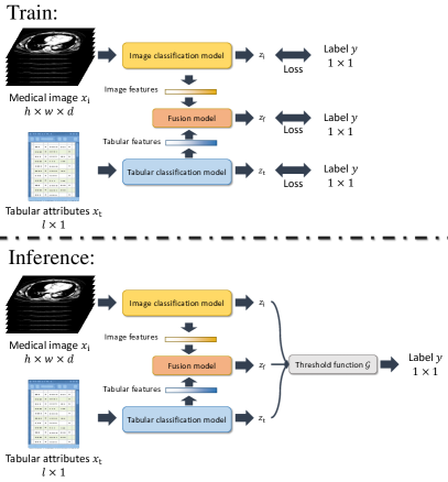
Figure 1: TNF’s overall structure. The input are medical image $\boldsymbol{x}_{\rm{i}}$ and corresponding tabular attributes $\boldsymbol{x}_{\rm{t}}$. $\boldsymbol{x}_{\rm{i}}$ and $\boldsymbol{x}_{\rm{t}}$ are inputted into image classification model and tabular classification model respectively to obtain likelihood $\boldsymbol{z}_{\rm{i}}$ and $\boldsymbol{z}_{\rm{t}}$. Image features and tabular features are inputted into fusion model to get likelihood $\boldsymbol{z}_{\rm{f}}$. $\boldsymbol{z}_{\rm{i}}$, $\boldsymbol{z}_{\rm{t}}$ and $\boldsymbol{z}_{\rm{f}}$ are processed by threshold function $\mathcal{G}$ to get the classification result $\hat{y}$.

In diagnosing certain diseases such as Alzheimer’s, clinicians use diagnostic tools combined with medical history and other information, including neurological exams, cognitive and functional assessments, medical imaging (MRI, CT, Ultrasound) and cerebrospinal fluid or blood tests to make an accurate diagnosis Association (2023). The aforementioned process will generate two modalities of medical data: one is medical image data including MRI, CT or Ultrasound images; another is medical tabular data including patient information such as gender, age and diagnostic results. For automatically diagnosing based on the medical image and tabular data, a multimodal medical data classification approach is desired. The classification method takes medical image and tabular data as input, and gives a diagnostic result as output.

In multimodal classification, there are conventionally two distinct approaches. The first is ensemble Rokach (2010); Kumar et al. (2016), which trains multiple models for different modalities, and ensembles the outputs of multiple models in the inference stage to obtain the final classification result. The second method is fusion, which extracts features of different modalities, then fuses the features and outputs the final classification result Zhang et al. (2021). Ensemble has higher robustness, but inferior in accuracy and interpretability than the fusion ones. Fusion has potentially higher accuracy, but easier to suffer from overfitting, and has lower flexibility (require all modalities to be available at both training and inference times). A method that can overcome the respective shortcomings of ensemble and fusion needs to be proposed.

In this paper, we propose Tri-branch Neural Fusion (TNF) for multimodal data classification shown in Fig. 1. Our method takes advantage of both ensemble and fusion. A medical image classification model classifies the medical image to obtain likelihood $z_{\rm{i}}$. A medical tabular classification model classifies medical tabular to obtain likelihood $z_{\rm{t}}$. At the same time, we fuse the features from the medical image classification model and the features from the medical tabular classification model to obtain likelihood $z_{\rm{f}}$. We ensemble likelihood $z_{\rm{i}}$, $z_{\rm{t}}$ and $z_{\rm{f}}$ to get the classification result.

Our TNF does not rely on a specific network structure. In the experiments, we validated our method by using a variety of pure convolutional neural network (CNN) structures and CNN+Transformer Vaswani et al. (2017) hybrid structures. We also validated our method on two image-tabular multimodal datasets: the pulmonary embolism (PE) dataset Zhou et al. (2021) which consists of PE CT scans and clinical records; as well as the cognitive impairment level classification dataset Beekly et al. (2004) which consists of brain MRI scans and questionnaire forms. Our method achieved superior performance than the ensemble method and the fusion method, improving the ACC, MCC Chicco et al. (2021), AUROC and other metrics by 1% to 5%. We also observed that, benefited from the fine-tuning process of TNF, the image branch and the tabular branch of TNF yielded better results than their single-modal counterparts. Additionally, during the inference stage, the TNF model can work even if one modality (either image or tabular) is missing. This shows TNF’s flexibility over traditional multimodal fusion methods, which require all types of data to be present for making predictions.

The contributions of this paper can be summarized as:

• We propose Tri-branch Neural Fusion (TNF), a high-performance classification structure that combines fusion and ensemble for multimodal medical data classification.

• We further propose two approaches named label masking and maximum likelihood selection to tackle the problem of label inconsistency in a multimodal classification task. These two methods achieved satisfying results on TNF-based models.

• Sufficient experiments on various Transformer and CNN structures proves that TNF is superior to individual fusion or ensemble. Experiments on multiple datasets demonstrate the generality of TNF.

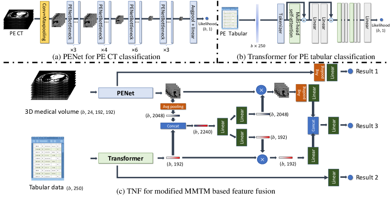
Figure 2: Classification models used in TNF for pulmonary embolism (PE) classification.

2 Related Works

2.1 Multi-modality in Medical Data Processing

A modality is a particular mode wherein something exists, is experienced, or is expressed Pei et al. (2023). For example, data regarding two datasets collected under two different circumstances, can be regarded as two modalities Baltrušaitis et al. (2018). In the field of machine learning for medical data, efforts have been made to emulate the multimodal nature of clinical expert decision-making to enhance prediction accuracy Su et al. (2020). The multi-modality medical data processing mainly focuses on classification, prediction and segmentation.

About classification, MRI and tabular data was utilized together for breast cancer classification Holste et al. (2021). Notably, the data in this study was exclusively collected from a single institution. Another study employed multiple imaging modalities for skin lesion classification Yap et al. (2018). However, its accuracy improvement over the baseline was found to be limited. About prediction, histology pathological images and genomics information were combined together for survival prediction Mobadersany et al. (2018). However, the dataset used in this study is relatively small. Additionally, Brain lesion patterns and user-defined clinical measurements were used for predicting conversion to multiple sclerosis Yoo et al. (2019). This method needs user-defined MRI measurements, necessitating collaboration with clinicians.

It is noteworthy that the aforementioned methods share three common limitations. First, they primarily concentrate on enhancing specific network structures, which may lack versatility across different machine learning architectures (e.g. unable to apply improvements designed for CNNs to Transformer models). Second, labels can vary between modalities. However, these methods require the labels of different modalities to be consistent for the training process. Third, these methods necessitate the availability of multi-modal inputs both during training and inference stages. If any modality is missing during the inference phase, these methods become inoperable. Our innovative approach effectively overcomes these three limitations.

2.2 Ensemble and Fusion Techniques in Multimodal Classification

Ensemble and fusion are two prevalent strategies in multimodal data classification. The ensemble approach combines outputs from multiple base classifiers, enhancing robustness and accuracy. This technique has been proven effective in RGB nature image classification Beluch et al. (2018) and medical image classification Zhou et al. (2021).

In contrast, fusion integrates data from multiple sources or modalities at different levels to enhance classification performance. It has been extensively applied in deep learning-based classification. In the context of CNN, the Multimodal Transfer Module (MMTM) Joze et al. (2020) implements fusion of feature modality within convolution layers in varying spatial dimensions. Weighted Feature Fusion Dong et al. (2022) merges features from Graph Attention Networks and CNNs for hyperspectral image classification. Auxiliary supervision Holste et al. (2023) generates additional sources during training to increase fusion on small datasets. Regarding Transformer-based fusion, Cross-Modal Attention Li and Li (2020) facilitates simultaneous attention to two distinct sequences or feature sets. TokenFusion Wang et al. (2022) identifies uninformative tokens, replacing them with projected and aggregated inter-modal features in multimodal classification tasks.

3 Methodology

3.1 Overview

Given a medical image represented as $\boldsymbol{x}_{\rm{i}}$ and a set of tabular attributes denoted as $\boldsymbol{x}_{\rm{t}}$, our approach yields three distinct outputs: $z_{\rm{i}}$, $z_{\rm{t}}$, and $z_{\rm{f}}$, all derived from a deep learning model denoted as $\mathcal{F}(\cdot)$. Here, $z_{\rm{i}}$ and $z_{\rm{t}}$ is derived from the medical image and the tabular attributes, respectively, and $z_{\rm{f}}$ corresponds to the fused features of both the medical image and tabular attributes. The relationship can be described as follows:

$$z_{\rm{i}},z_{\rm{t}},z_{\rm{f}}=\mathcal{F}(\boldsymbol{x}_{\rm{i}},\boldsymbol{x}_{\rm{t}}),$$ (1)

during the training phase, the model $\mathcal{F}(\cdot)$ is optimized using a loss function $\mathcal{L}$, defined as:

$$\mathcal{L}=\lambda_{1}\mathcal{L}_{\rm{c}}(z_{\rm{i}},y_{\rm{i}})+\lambda_{2}\mathcal{L}_{\rm{c}}(z_{\rm{t}},y_{\rm{t}})+\lambda_{3}\mathcal{L}_{\rm{c}}(z_{\rm{f}},y_{\rm{f}}),$$ (2)

where $\lambda_{1}$, $\lambda_{2}$, and $\lambda_{3}$ are the weighting coefficients, $y_{\rm{i}}$, $y_{\rm{t}}$ and $y_{\rm{f}}$ are labels of the image, tabular and fusion branch, and $\mathcal{L}_{\rm{c}}(\cdot)$ represents the cross-entropy loss. In the inference phase, the classification result is determined by:

$$\hat{y}=\mathcal{G}\left(\frac{z_{\rm{i}}+z_{\rm{t}}+z_{\rm{f}}}{3}\right),$$ (3)

with $\mathcal{G}(\cdot)$ being a threshold function defined by a threshold $\theta$. For binary classification scenarios, this function is expressed as:

$$\mathcal{G}(z) =1,\quad\text{if }\alpha\geq\theta,$$ (4)

$$\mathcal{G}(z) =0,\quad\text{if }\alpha<\theta,$$ (5)

and commonly $\theta=0.5$. The complete framework of this method is illustrated in Fig.  1.

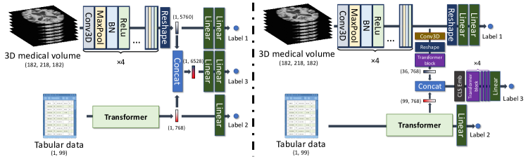
Figure 3: Models utilized in TNF for cognitive impairment level classification on the NACC dataset.

3.2 TNF for Pulmonary Embolism (PE) Classification

3.2.1 Backbone

We employed the Stanford AIMI pulmonary embolism (PE) dataset Zhou et al. (2021) as the first dataset in our study. This dataset comprises computed tomography (CT) scans and corresponding clinical data extracted from the electronic health records (EHR) of the same patients. We chose benchmark architectures: for the classification of CT scans, we utilized the PENet architecture Huang et al. (2020), and for the EHR data classification, we employed the Tabular Transformer Gorishniy et al. (2021). The integration of these methods in our framework is depicted in Fig. 2.

3.2.2 Training with Inconsistent Labels in Multimodal Fusion

Addressing label inconsistency is crucial in multimodal classification. In the PE dataset, each CT scan slice has its own label. For instance, a CT volume of size 256$\times$256$\times$100 yields 100 individual slice labels. However, the corresponding EHR data, is assigned only one single label, either positive or negative. Previous study Huang et al. (2020) established a benchmark for classifying PE dataset image data, dividing the CT volume into multiple 24 consecutive slices. If any 4 slices within any 24 consecutive slices are identified as positive, the entire volume is labeled positive. This approach does not completely solve the label inconsistency problem when fusing EHR and CT volume data, as the EHR label might not align with the image’s. Refer to Appendix A for details.

To resolve this discrepancy, we propose two approaches: 1) label masking, and 2) maximum likelihood selection.

$\bullet$ Label Masking The implementation of label masking can be described as;

$$\mathcal{L}=\begin{cases}\lambda_{1}\mathcal{L}_{\rm{c}}(z_{\rm{i}},y_{\rm{i}})+\lambda_{2}\mathcal{L}_{\rm{c}}(z_{\rm{t}},y_{\rm{t}})+\lambda_{3}\mathcal{L}_{\rm{c}}(z_{\rm{f}},y_{\rm{i}}),&\text{if }y_{\rm{i}}=y_{\rm{t}},\\ \lambda_{1}\mathcal{L}_{\rm{c}}(z_{\rm{i}},y_{\rm{i}})+\lambda_{2}\mathcal{L}_{\rm{c}}(z_{\rm{t}},y_{\rm{t}}),&\text{otherwise},\end{cases}$$ (6)

where $y_{\rm{i}}$ and $y_{\rm{t}}$ are labels of image and tabular, respectively. The fusion branch’s weights will be optimized only if $y_{\rm{i}}=y_{\rm{t}}$. With label masking, the training of fusion branch will not be conducted if the labels are inconsistent.

$\bullet$ Maximum Likelihood Selection We use pre-trained PENet in previous research Zhou et al. (2021) to extract the 24 slices with the highest likelihood for each volume, and use these 24 slices as input to train TNF-based models. If the entire volume is positive, then these 24 slices are also positive, otherwise they are negative.

This process can be described as,

$$j^{\prime}=\mathop{\rm argmax}\limits_{j}(\mathcal{F}_{\rm{i}}(\boldsymbol{x}^{j}_{\rm{i}})),\quad j\in\{1,\ldots,N\},$$ (7)

$$z_{\rm{i}},z_{\rm{t}},z_{\rm{f}}=\mathcal{F}(\boldsymbol{x}^{j^{\prime}}_{\rm{i}},\boldsymbol{x}_{\rm{t}}),$$

where $N$ represents the total number of 24-slice groups within a CT volume. For example, if a CT volume contains 100 slices, $N=\left\lceil{\frac{100}{24}}\right\rceil=5$. This means there are five groups, with Groups 1 to 4 each comprising 24 slices, and Group 5 containing only 4 slices. We use padding by filling Group 5 with the CT value of air (-1000), expanding it from 4 to 24 slices. $\mathcal{F}_{\rm{i}}$ is the PENet in Fig. 2 (a). By only selecting the slices that with the highest positive likelihood, maximum likelihood selection solves the inconsistency problem between image and tabular labels.

3.2.3 TNF-Based Models for PE Classification

We validated several models based on TNF for PE classification.

$\bullet$ MMTM-based Feature Fusion First, we conducted experiments based on TNF for MMTM-based feature fusion. MMTM Joze et al. (2020) is a widely-used feature fusing method for fusing the knowledge of multiple modalities like

$$\begin{split}\boldsymbol{v}_{\rm{a}}^{\prime}=&\boldsymbol{v}_{\rm{a}}\odot f_{\rm{a}}(f_{\rm{c}}(C(\mathcal{S}(\boldsymbol{v}_{\rm{a}}),\mathcal{S}(\boldsymbol{v}_{\rm{b}}))),\\ \boldsymbol{v}_{\rm{b}}^{\prime}=&\boldsymbol{v}_{\rm{b}}\odot f_{\rm{b}}(f_{\rm{c}}(C(\mathcal{S}(\boldsymbol{v}_{\rm{a}}),\mathcal{S}(\boldsymbol{v}_{\rm{b}}))),\end{split}$$ (8)

where $\mathcal{S}$ is the “squeeze” function to squeeze multi-dimension feature $\boldsymbol{v}_{\rm{a}},\in\mathbb{R}^{b\times c\times m_{1},...,m_{K}}$ to $\mathbb{R}^{b\times c}$. $f_{\rm{a}}(\cdot)$ and $f_{\rm{b}}(\cdot)$ and $f_{\rm{c}}(\cdot)$ are linear layers respectively. $C(\cdot)$ is channel-wise concatenation. $\odot$ is channel-wise multiply.

In our context, features $\boldsymbol{v}_{\rm{i}}\in\mathbb{R}^{b\times c\times h\times w\times d}$ are obtained from a 3D medical volume, while the features $\boldsymbol{v}_{\rm{t}}\in\mathbb{R}^{b\times l}$ are derived from a Tabular Transformer. Due to the differing dimensions of these features, where $\boldsymbol{v}_{\rm{t}}$ from the Tabular Transformer has only two dimensions, squeezing $\boldsymbol{v}_{\rm{t}}$ is deemed unnecessary. Consequently, we adapted the MMTM method to fuse $\boldsymbol{v}_{\rm{i}}$ and $\boldsymbol{v}_{\rm{t}}$, as illustrated in Fig. 2 (c). The modified fusion process is defined as:

$$\begin{split}\boldsymbol{v}_{\rm{i}}^{\prime}=&\boldsymbol{v}_{\rm{i}}\odot f_{\rm{i}}(f_{\rm{c}}(C(f_{\rm{avg}}(\boldsymbol{v}_{\rm{i}}),\boldsymbol{v}_{\rm{t}}))),\\ \boldsymbol{v}_{\rm{t}}^{\prime}=&\boldsymbol{v}_{\rm{t}}\odot f_{\rm{t}}(f_{\rm{c}}(C(f_{\rm{avg}}(\boldsymbol{v}_{\rm{i}}),\boldsymbol{v}_{\rm{t}}))),\end{split}$$ (9)

where $f_{\rm{avg}}$ is average pooling function. Subsequently, the fused output is obtained through a process of average pooling, concatenation, and application of a linear layer, as depicted in Fig. 2 (c).

$\bullet$ Concatenation-Based Transformer Feature Fusion The effectiveness of TNF was also evaluated on Transformer structures. For image features $\boldsymbol{v}_{\rm{i}}\in\mathbb{R}^{b\times c\times h\times w\times d}$, we apply 3D convolution and a reshaping function to transform them into $\boldsymbol{v}_{\rm{i}}^{\prime}\in\mathbb{R}^{b\times h\times w\times d\times c^{\prime}}$. These features are then concatenated channel-wise with outputs from the Tabular Transformer. The likelihood is calculated as follows:

$$\begin{split}z_{f}=\mathcal{T}(C(\boldsymbol{v}_{\rm{i}}^{\prime},\boldsymbol{v}_{\rm{t}})),\end{split}$$ (10)

where $\mathcal{T}$ represents the class embedding and Transformer blocks. Refer to Appendix B for detailed network structure.

$\bullet$ TokenFusion-Based Transformer Feature Fusion: TNF also demonstrates effectiveness with TokenFusion Wang et al. (2022) and Cross-Modal Attention Li and Li (2020) in Transformer feature fusion. We use TokenFusion to fuse features from image and tabular modalities:

$$\boldsymbol{v}_{\rm{i}}^{\prime} =\boldsymbol{v}_{\rm{i}}+\rm{MLP}((\rm{SA}(\boldsymbol{v}_{\rm{i}})\odot\it{f}(\boldsymbol{v}_{\rm{i}}))+\boldsymbol{v}_{\rm{i}}),$$ (11)

$$\boldsymbol{v}_{\rm{t}}^{\prime} =\boldsymbol{v}_{\rm{t}}+\rm{MLP}((\rm{SA}(\boldsymbol{v}_{\rm{t}})\odot\it{f}(\boldsymbol{v}_{\rm{t}}))+\boldsymbol{v}_{\rm{t}}),$$

where $\rm{MLP}$ is a multi-layer perceptron, $\rm{SA}$ is a self-attention mechanism, and $f(\cdot)$ is a linear function. Afterwards, $\boldsymbol{v}_{\rm{i}}^{\prime}$ and $\boldsymbol{v}_{\rm{t}}^{\prime}$ will be fused to get the classification result. TokenFusion assigns weights to each token, selectively emphasizing or de-emphasizing certain tokens.

$\bullet$ Cross-Modal Attention-Based Transformer Feature Fusion: On the other hand, Cross-Modal Attention facilitates simultaneous attention to two distinct feature sources:

$$\boldsymbol{v}_{\rm{i}}^{\prime} =\rm{MA}(\mathcal{Q}_{t}(\boldsymbol{v}_{\rm{t}}),\mathcal{K}_{i}(\boldsymbol{v}_{\rm{i}}),\mathcal{V}_{i}(\boldsymbol{v}_{\rm{i}})),$$ (12)

$$\boldsymbol{v}_{\rm{t}}^{\prime} =\rm{MA}(\mathcal{Q}_{i}(\boldsymbol{v}_{\rm{i}}),\mathcal{K}_{t}(\boldsymbol{v}_{\rm{t}}),\mathcal{V}_{t}(\boldsymbol{v}_{\rm{t}})),$$

where $\rm{MA}$ represents a multi-head attention mechanism, while $\mathcal{Q}$, $\mathcal{K}$, and $\mathcal{V}$ denote the query, key, and value operations.

3.3 TNF for Cognitive Impairment Level Classification

TNF was also employed for a multi-class classification task involving cognitive impairment level classification using the NACC Beekly et al. (2004) dataset. The cognitive impairment levels are categorized into three stages: 0 (normal), 1 (mild cognitive impairment), and 2 (severe cognitive impairment). The NACC dataset comprises two types of modalities: brain MRI volumes (image data) and questionnaire forms (tabular data). We developed two models based on TNF for classifying NACC data.

3.3.1 Concatenation-Based Feature Fusion

The first model, depicted in Fig. 3 (a), employs a CNN for classifying brain MRI volumes and a Tabular Transformer for processing tabular data. We concatenate the features from the brain MRI volume, with a shape of $(b,5760)$, with those from the Tabular Transformer, with a shape of $(b,768)$. This results in a combined feature vector of shape $(b,6528)$, which is then fed into linear layers to derive the fusion label.

3.3.2 Transformer Feature Fusion

The second model, shown in Fig. 3 (b), involves processing features from the brain MRI volume through a 3D convolution layer, a reshaping operation, and a Transformer block. This process yields a feature vector of shape $(b,36,768)$. Features from the intermediate layers of the Tabular Transformer, shaped $(b,99,768)$, are then concatenated with this vector to form a new vector of shape $(b,135,768)$. This combined vector is subsequently inputted into Transformer layers to obtain the fusion label.

	Label masking		Maximum likelihood selection
	w/o Pre-train	w/ pre-train	w/o Pre-train	w/ pre-train
AUPRC $\uparrow$	0.871	0.887	0.844	0.910
AUROC $\uparrow$	0.818	0.845	0.797	0.867
ACC $\uparrow$	0.747	0.768	0.742	0.789
MCC $\uparrow$	0.477	0.529	0.464	0.582
Recall $\uparrow$	0.891	0.782	0.827	0.764

Table 1: Comparison of maximum likelihood selection and label masking on PE dataset w/ and w/o pre-training.

	Single modal		Multimodal		Ensemble	TNF + maximum likelihood selection
	Img only	Tab only	MMTM fusion1	Clip fusion	Img+Tab	MMTM	Concatenation	TokenFusion	CM Attention2
AUPRC $\uparrow$	0.848	0.842	0.861	0.838	0.888	0.910	0.907	0.905	0.895
AUROC $\uparrow$	0.786	0.788	0.816	0.797	0.847	0.867	0.865	0.860	0.848
ACC $\uparrow$	0.716	0.737	0.721	0.705	0.774	0.789	0.779	0.784	0.789
MCC $\uparrow$	0.407	0.472	0.455	0.393	0.534	0.582	0.567	0.567	0.567
Recall $\uparrow$	0.855	0.727	0.673	0.918	0.818	0.764	0.736	0.773	0.827

• Structure is equivalent to the model in Fig. 2 (c) while only outputs fusion result.

• “Cross-Modal Attention-Based Transformer Feature Fusion” in Section 3.2.

Table 2: Results on PE dataset.

	Single modal		Multimodal	Ensemble	TNF
	Img	Tab	Fusion	Img+Tab	Model 11	Model 22
ACC $\uparrow$	0.669	0.761	0.653	0.785	0.785	0.805
MCC $\uparrow$	0.509	0.564	0.381	0.623	0.629	0.672
Recall $\uparrow$	0.657	0.624	0.488	0.667	0.682	0.712
Jaccard $\uparrow$	0.480	0.516	0.342	0.544	0.552	0.580
F1 $\uparrow$	0.640	0.655	0.431	0.677	0.686	0.709

• “Concatenation-Based Feature Fusion” and “Transformer Feature Fusion” models in Section 3.3, respectively.

Table 3: Results on NACC dataset. Since AUPRC and AUROC are not applicable to a multi-classification problem, we added Jaccard and macro F1 score as additional metrics.

	Img branch	Tab branch	Fusion	Ensemble1	TNF
AUPRC $\uparrow$	0.864	0.840	0.849	0.910	0.910
AUROC $\uparrow$	0.792	0.790	0.799	0.865	0.867
ACC $\uparrow$	0.684	0.705	0.768	0.768	0.789
MCC $\uparrow$	0.437	0.405	0.474	0.561	0.582
Recall $\uparrow$	0.536	0.709	0.764	0.691	0.764

• The ensemble of Img and Tab branch after TNF fine-tuning.

Table 4: Performance of each branch of TNF models on PE dataset.

4 Experiments and Results

4.1 Preprocessing

4.1.1 Preprocessing of PE Dataset

The tabular of PE dataset contains 1,505 attributes such as age, gender, pulse, etc. We remove two attributes that are directly related to PE (“DISEASES OF PULMONARY CIRCULATION: frequency” and “DISEASES OF PULMONARY CIRCULATION: presence”) because we found if these two attributes are not 0, PE must be positive. We use SHAP Shrikumar et al. (2017) to select the most important 250 attributes for PE classification.

We also resized images from PE dataset from size 256$\times$256 to 224$\times$224, and center-cropped their size to 192$\times$192. We normalized the image intensity to range [-1, 1].

4.1.2 Preprocessing of NACC Dataset

$\bullet$ Case Selection and Image Preprocessing The NACC dataset contains 9,812 case of brain MRI with T1, T2 and FLAIR modality. We select thin-slice cases that have T1 modality and use FreeSurfer Fischl (2012) to perform bone removal, resize and intensity normalization. After preprocessing, there remain 1,252 cases with size 182$\times$218$\times$182 voxels. We normalized the volume intensity to range [-8, 8].

$\bullet$ Tabular Preprocessing We preprocessed NACC tabular data by zero padding, feature selection and normalization. After preprocessing, the tabular data was left with 99 features including cognitive questionnaire information, gender, age, etc.

4.2 Training and Inference

4.2.1 PE Dataset

We follow the experimental settings of the PE dataset Zhou et al. (2021). There are totally 1,837 cases, 1,454 cases for training, 190 cases for validation, and 193 cases for testing.

We loaded the best pre-trained PENet provided by prior research Huang et al. (2020). To ascertain the saturation of the pre-trained weights, we ran additional training epochs starting from the pre-trained weights, and confirmed no further improvement in performance; we loaded pre-trained Tabular Transformer trained by ourselves, to TNF-based models for training. The learning rate is 10^-4 with cosine decay down to 10^-5. The number of epoch is 1,000, the optimizer is AdamW Loshchilov and Hutter (2018). The regularization parameters are set as $\lambda_{1}=0.1$, $\lambda_{2}=0.1$, $\lambda_{3}=0.8$. The best model on the validation dataset was used for testing.

4.2.2 NACC Dataset

Among the 1,252 cases of the NACC dataset, we randomly selected 752 cases for training, 249 cases for validation and 251 cases for testing.

We pre-trained a 4-block CNN model consistent with the architecture used in previous research Qiu et al. (2022), as shown in Fig. 3, for image classification; and a Tabular Transformer model with the same structure in Fig. 2 (b) for tabular classification. After pre-training, we train TNF-based models shown in Fig. 3 (a) (b). The learning rate is 10^-3, epoch is 100, and the optimizer is Adam.

4.3 Results

4.3.1 PE Dataset

First, we evaluated two approaches on the PE dataset: training with inconsistent labels using maximum likelihood selection against label masking, and comparing training from scratch against pre-training. For the case of training from scratch, only the PENet was pre-trained on the Kinetics-600 dataset Carreira et al. (2018). For the case of pre-training, both the PENet and the Tabular Transformer were pre-trained on the PE dataset. The outcomes of these comparisons are presented in Table 1. We found that the combination of maximum likelihood selection and pre-training yielded the best performance across most metrics. Therefore, we select it for the following experiments.

The results for the PE dataset are detailed in Table 2, with the ROC curve displayed in Fig. 4. We compared TNF-based models with single modal, multimodal fusion, and ensemble approaches. We tried two fusion models: 1) MMTM fusion, whose structure is equivalent to the model in Fig. 2 (c) while only outputs fusion result. 2) Clip fusion, based on the research of Hager et al. (2023) (refer to Appendix C for details). The TNF approach not only surpassed single-modal classification (using either image or tabular) but also outperformed multimodal fusion and ensemble in most metrics. Notably, the fusion approach demonstrated lower accuracy compared to the ensemble method, indicating that conventional multimodal fusion may be ineffective for some datasets.

4.3.2 NACC Dataset

The quantitative results for the NACC dataset are presented in Table 3. For comparison, the multimodal fusion model is identical to the model with only the fusion branch, as shown on the left in Fig. 3. Our two TNF-based models, namely the simple concatenation-based feature fusion and the Transformer feature fusion model, demonstrated superior performance compared to other methods.

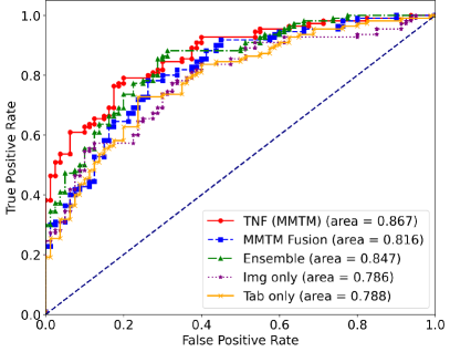
Figure 4: ROC curve of TNF and other methods.

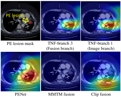
Figure 5: Grad-CAM heatmaps (zoom in for better observation).

4.4 3D Grad-CAM-based Critical Region Analysis

To visualize the critical regions for the models’ predictions, we designed a 3D Grad-CAM model and adapted it to the TNF models. Grad-CAM Selvaraju et al. (2017) produces visual explanations for decisions made by CNNs. We modified Grad-CAM so that it can be applied to multiple inputs and multiple outputs, as well as can process 3D medical images. We back-propagate one output at a time to get its Grad-CAM heatmaps.

We compared five types of Grad-CAM heatmaps: 1) The fusion branch of TNF. the model is shown in Fig. 2 (c); 2) The image branch of TNF; 3) PENet; 4) MMTM fusion model; The model’s structure is equivalent to the model in Fig. 2 (c) and only outputs fusion result; 5) Clip fusion model.

The Grad-CAM heatmaps are compared with PE lesion masks marked by clinicians shown in Fig. 5 as an exmaple. TNF’s Grad-CAM heatmap highlighted the lesion area. On the other hand, PENet’s heatmap highlighted a larger area. MMTM fusion and Clip fusion failed to highlight the lesion. Generally, TNF’s heatmap is the closest to the lesion mask.

4.5 Performance of Each Branch of TNF Models

We also conducted performance comparison of individual branches of TNF models, shown in Table 4. Note that our TNF model has three branches: 1) the image branch; 2) the tabular branch; and 3) the fusion branch. We illustrated the results of each individual branch, the ensemble of the first two branches, as well as TNF. TNF achieved the best quantitative results, except for recall.

5 Discussion

	Tabular Transformer		ElasticNet		ResNet
	Tab	Ensemble	Tab	Ensemble	Tab	Ensemble
AUROC $\uparrow$	0.788	0.847	0.783	0.829	0.750	0.847
ACC $\uparrow$	0.737	0.774	0.626	0.784	0.684	0.716
MCC $\uparrow$	0.472	0.534	0.349	0.562	0.403	0.459

Table 5: Different model’s performance on tabular data classification on PE dataset. Generally, Tabular Transformer is the best.

5.1 Comparison of Label Masking and Maximum Likelihood Selection

To address the challenge of inconsistent labels in multimodal processing, we introduce two approaches: label masking and maximum likelihood selection. According to the results in Table 1, maximum likelihood selection achieves higher AUPRC compared to label masking (0.910 vs. 0.887) when the network is pre-trained. However, without pre-training, the situation is reversed (0.844 vs. 0.871). This indicates that maximum likelihood selection is more effective for fine-tuning a pre-trained network as it does not add new label information, which might be redundant at the stage of training. Conversely, label masking is preferable for training from scratch, as it introduces a larger amount of training data.

5.2 Model Selection for Tabular Classification

ElasticNet Zou and Hastie (2005) was previously used for tabular data classification in the PE dataset. We additionally explored ResNet Jian et al. (2016) and the Tabular Transformer Gorishniy et al. (2021) to evaluate their effectiveness. Table 5, indicated that the Tabular Transformer outperformed other models. Consequently, we chose the Tabular Transformer as our baseline model.

5.3 TNF Enhances Single Modal Classification

The “Img branch” column in Table 4 and the “Img only” column in Table 2 display the results of image classification. Following fine-tuning with the TNF, there was an observable improvement in the performance metrics for image classification. AUPRC increased from 0.848 to 0.864, and the MCC increased from 0.407 to 0.437. We attribute this enhancement to the integration of table modality features in the fusion process. TNF enables the PENet to more effectively extract common features crucial for accurate classification.

5.4 TNF’s Advantages over Multimodal Fusion

When information from different modalities conflicts, using the fusion method will actually reduce the accuracy. As shown in Table 2 and Table 3, multimodal fusion cannot outperform ensemble. This is partly because if the fusion part is optimized, the feature extraction part may be poorly optimized. TNF solved this problem by extracting common features between modalities while maintaining optimization of the feature extraction part. Another advantage of TNF over fusion is that it can still infer the result while one modality is missing. For instance, if tabular data is missing, we can still infer the result by using the image branch. On the other hand, multimodal fusion models cannot infer the result while one modality’s data is missing.

6 Conclusion

We proposed Tri-branch Neural Fusion (TNF) model for multimodal data classification. We also proposed label masking and maximum likelihood selection to address the challenge of inconsistent labels. We validated TNF model on various CNN and Transformer-based fusion algorithms on two multimodal medical datasets, all of which outperformed multimodal ensemble and fusion results. Compared with multimodal fusion, TNF can still infer the classification result when a certain mode is missing. Relative to ensemble, TNF achieved better quantitative results. Grad-CAM-based interpretability studies further proved that TNF can allow the model to focus on lesions, thus demonstrating its potential in auxiliary diagnosis. In the future, we plan to explore the case of more than two modalities fusion, as well as introduce TNF-based models into clinical practice to provide support to clinicians.

Appendix for TNF: Tri-branch Neural Fusion for Multimodal Medical Data Classification
   

A Details About Maximum Likelihood Selection and Label Masking

A.1 Label Inconsistency Problem

Inconsistencies may arise between EHR labels and image labels within the PE dataset as shown in Table A. Huang et al. Huang et al. (2020) set a classification benchmark for PE image data by segmenting the CT volume into groups, with each containing 24 consecutive slices. A volume is deemed positive if at least 4 slices in any of these groups are positive. Our study adheres to this approach.

However, a positive PE volume doesn’t guarantee that all its slices are positive. Actually, according to Table A, for all the volumes which are annoted as positive, only 15.27% slices are positive, and only 19.06% 24-slice groups are positive. This discrepancy leads to label inconsistencies when comparing positive EHR data with potentially negative image groups. We propose 1) label masking, and 2) maximum likelihood selection to tackle this problem.

A.2 Maximum Likelihood Selection

We use pre-trained PENet in previous research Zhou et al. (2021) to extract the 24 slices with the highest likelihood for each volume, and use these 24 slices as input to train TNF-based models. The procedure is illustrared in Algorithm 1.

Algorithm 1 Maximum Likelihood Selection

$\mathbb{X}$: All volumes in the PE dataset

$\mathcal{F}$: Pre-trained PENet

$\boldsymbol{X}_{j}$: $j_{\rm{th}}$ volume of $192\times 192\times K$ voxels

procedure MLS($\mathbb{X},\mathcal{F}$)

     $\mathbb{V}\leftarrow[]$

     for each volume $\boldsymbol{X}_{j}\in\mathbb{X}$ do

         $L\leftarrow[]$ $\triangleright$ likelihood list

         Divide $\boldsymbol{X}_{j}$ into $\boldsymbol{x}_{j1},\boldsymbol{x}_{j2},\ldots,\boldsymbol{x}_{jN}$ of size $192\times 192\times 24$

         for each $\boldsymbol{x}_{jn}$ do

              $l\leftarrow\mathcal{F}(\boldsymbol{x}_{jn})$ $\triangleright$ get likelihood from PENet

              Append $l$ to $L$

         end for

         $\text{Idx}\leftarrow\text{argmax}(L)$

         Append $\boldsymbol{x}_{j\text{Idx}}$ to $\mathbb{V}$

     end for

     Use $\mathbb{V}$ to train TNF-based models

end procedure

Algorithm 2 Label Masking

$\boldsymbol{x}_{\text{i}},\boldsymbol{x}_{\text{t}}$: Image and tabular data

$y_{\text{i}},y_{\text{t}}$: The corresponding labels of the image and tabular data

$\mathcal{L}_{\rm{c}}$: Cross-entropy loss function

$N$: Size of mini-batch

procedure LM($\boldsymbol{x}_{\text{i}},\boldsymbol{x}_{\text{t}},y_{\text{i}},y_{\text{t}}$)

     for $n=1$ to $N$ do

         if $y_{\text{i}}^{n}=y_{\text{t}}^{n}$ then

              $\mathcal{L}^{n}=\lambda_{1}\mathcal{L}_{\rm{c}}(z_{\rm{i}}^{n},y_{\rm{i}}^{n})+\lambda_{2}\mathcal{L}_{\rm{c}}(z_{\rm{t}}^{n},y_{\rm{t}}^{n})+\lambda_{3}\mathcal{L}_{\rm{c}}(z_{\rm{f}}^{n},y_{\rm{i}}^{n})$

         else

              $\mathcal{L}^{n}=\lambda_{1}\mathcal{L}_{\rm{c}}(z_{\rm{i}}^{n},y_{\rm{i}}^{n})+\lambda_{2}\mathcal{L}_{\rm{c}}(z_{\rm{t}}^{n},y_{\rm{t}}^{n})$

         end if

     end for

     $\mathcal{L}_{\text{total}}=\frac{1}{N}\sum_{n=1}^{N}\mathcal{L}^{n}$

     Use $\mathcal{L}_{\text{total}}$ to train TNF-based models

end procedure

A.3 Label Masking

With label masking, the training of fusion branch will not be conducted if the label is inconsistent. The procedure is illustrated in Algorithm 2.

For example, in a multimodal classification problem, if the labels of image and tabular data are inconsistent, it can be divided into the following two situations:

1. The labels of image and tabular are the same. Train the image, tabular, and fusion branches in the TNF-based models.

2. The labels of image and tabular are different. Only train the image and tabular branches in the TNF-based models.

	Single slice		24 slices
	Img=1	Img=0	Img=1	Img=0
Tab=1	44,071	244,591	2,361	10,025
Tab=0	0	433,956	0	18,608

Table A: Label inconsistency problem in the PE dataset: Each slice (image) within CT volumes is individually labeled, whereas the corresponding EHR data (tabular) for the entire CT volume has a single label, leading to situations where some image labels are 0 while the corresponding EHR data label is 1.

B Details of TNF-Based Models for PE Classification

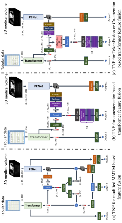
Figure A: TNF-based networks on PE dataset.

In order to verify the generalization of TNF, We tried serval models based on TNF for PE classification. Here we present the details of these models.

B.1 Modified MMTM-based feature fusion

Initially, we carried out experiments utilizing TNF with a modified MMTM-based feature fusion approach. We employed MMTM to integrate features from image and tabular data, followed by the application of a linear layer to obtain the output of the fusion branch. The architecture of this model is illustrated in Fig. A (a).

B.2 Transformer Feature Fusion

Concatenation-Based Feature Fusion We also assessed the concatenation-based feature fusion of TNF on transformer architectures. In this approach, we processed the image CNN features from PENet through a transformer block to obtain transformer features, which were then concatenated with features from the tabular transformer. Subsequently, these combined features were processed through 8 transformer blocks to derive the output of the fusion branch, as illustrated in Fig. A (b).

TokenFusion and Cross-Modal Attention-Based Feature Fusion The architectures of models based on TokenFusion Wang et al. (2022) and Cross-Modal Attention Li and Li (2020) are presented in Fig. A (c). For fusing image and tabular features, we employed either TokenFusion or Cross-Modal Attention. These fused features were then processed through 8 transformer blocks to produce the output of the fusion branch.

C Details of CLIP Fusion in the “Experiments” Section

We employed a multimodal fusion approach shown in Fig. B inspired by the work of Hager et al. Hager et al. (2023), which itself is based on the principles derived from CLIP radford2021learning. We employed CLIP loss for fine-tuning our pretrained models, leveraging CLIP’s exceptional performance not only in pre-training phases but also in fine-tuning scenarios, as highlighted by Dong et al. dong2022clip. The training and inference processes are outlined as follows:

• Start with pre-trained models: PENet for PE images and a Tabular Transformer for EHR data.

• Proceed to fine-tune both the PENet and the Tabular Transformer using a hybrid loss function that combines cross-entropy and CLIP losses. The loss function is articulated as:

  $$\begin{split}\mathcal{L}&=\lambda_{1}\mathcal{L}_{\rm{c}}(z_{\mathrm{i}},y)+\lambda_{2}\mathcal{L}_{\rm{c}}(z_{\mathrm{t}},y)\\ &+\lambda_{3}\left(0.5\mathcal{L}_{\rm{p}}(f_{\mathrm{i}},f_{\mathrm{t}})+0.5\mathcal{L}_{\rm{p}}(f_{\mathrm{t}},f_{\mathrm{i}})\right),\end{split}$$ (13)

  where $\lambda_{1}=0.1$, $\lambda_{2}=0.1$, and $\lambda_{3}=0.8$ are the weighting coefficients. Here, $f_{\mathrm{i}}$ and $f_{\mathrm{t}}$ denote features extracted by the PENet and Tabular Transformer, respectively. $\mathcal{L}_{\rm{c}}$ represents the cross-entropy loss, and $\mathcal{L}_{\rm{p}}$ denotes the CLIP loss, which is defined as

  $$\mathcal{L}_{\rm{p}}(f_{\mathrm{i}},f_{\mathrm{t}})=-\sum_{j\in N}\log\frac{\exp(\cos(f_{ji},f_{jt})/\tau)}{\sum_{k\in N,k\neq j}\exp(\cos(f_{ji},f_{kt})/\tau)},$$ (14)

  where $N=8$ is the batch size and $\tau$ is set to 0.9995. The CLIP loss encourages the model to align images and tabular data features from the same case, while differentiating between features from different cases by minimizing or maximizing their cosine similarity.

• Conduct inference using the fine-tuned PENet and Tabular Transformer. We present three categories of results: (1) ensemble using outputs from both image and tabular data, (2) inference based on image data alone, and (3) inference based on tabular data alone.

Experimental results demonstrated in Table B indicate that single modality and ensemble surpassed the performance of CLIP fusion. The fact suggests that the efficacy of fusion methods is dependent on the datasets used. Some datasets contain multimodal data with high inter-modality correlation, which enhances the performance of fusion-based approaches. Conversely, in datasets where the multimodal data are relatively independent, fusion methods may not yield improvements.

	CLIP fusion			Single modality & ensemble
	Ensemble	Img only	Tab only	Ensemble	Img only	Tab only
AUPRC $\uparrow$	0.838	0.816	0.832	0.888	0.848	0.842
AUROC $\uparrow$	0.797	0.734	0.770	0.847	0.786	0.788
ACC $\uparrow$	0.705	0.663	0.621	0.774	0.716	0.737
MCC $\uparrow$	0.393	0.291	0.202	0.534	0.407	0.472
Recall $\uparrow$	0.918	0.882	0.964	0.818	0.855	0.727

Table B: Performance comparison of models w/ and w/o CLIP fusion. CLIP fusion lead to a decline in most metrics.

Figure B: Process of CLIP fusion is adapted from Hager et al. Hager et al. (2023). During the training phase, we fine-tune both the PENet and the Tabular Transformer by employing a combination of cross-entropy loss and CLIP loss. For the inference phase, we utilize the fine-tuned PENet and Tabular Transformer to perform predictions.

D SHAP-based Attribute Selection

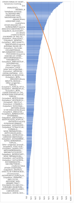
Figure C: Top 250 influential attributes of the PE dataset’s EHR tabular data.

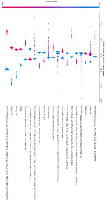
Figure D: Closer examination of the top 20 attributes, along with their levels of contribution of the PE dataset’s EHR tabular data.

Attributes	1503	1000	500	250	100
AUROC	0.727	0.697	0.693	0.788	0.777
ACC	0.694	0.705	0.684	0.737	0.737
MCC	0.390	0.421	0.403	0.472	0.467

Table C: Impact of selecting different number of tabular attributes on the PE dataset

To enhance our classification model performance on the PE dataset, we applied SHAP (SHapley Additive exPlanations) Lundberg and Lee (2017) to identify the top 250 most impactful attributes from an initial set of 1,503 tabular attributes—down from 1,505 after excluding two directly related to PE. SHAP values, which are grounded in cooperative game theory, assign an importance score to each attribute based on its contribution to the model’s prediction.

The formula to calculate SHAP values is given by:

$$\phi_{i}=\sum_{S}\frac{|S|!(|F|-|S|-1)!}{|F|!}[f(S\cup\{i\})-f(S)],$$ (15)

where $\phi_{i}$ is the SHAP value for feature $i$, $F$ is the total set of features, and $S$ is a subset of features excluding $i$.

The results, presented in Table C, indicate that a subset of 250 attributes yielded superior classification accuracy compared to larger or smaller subsets of attributes. Illustrations of the top 250 influential attributes are provided in Fig. C, and a closer examination of the top 20 attributes, along with their levels of contribution, is depicted in Fig. D.

E Preprocessing of NACC Dataset

Case Selection and Image Preprocessing As detailed in the paper, the NACC dataset Beekly et al. (2004) comprises 9,812 brain MRI cases featuring T1, T2, and FLAIR modalities. For the detection of cognitive impairment, the T1 modality is commonly preferred zamani2022diagnosis. The MRI cases selected for deep-learning classification adhered to the following criteria:

• Inclusion of the T1 modality.

• Availability of high-resolution, thin-slice MRI scans.

• Accompanying tabular data encompassing cognitive assessments, gender, age, and other relevant information.

Following these criteria, we narrowed down the NACC dataset to 1,252 cases.

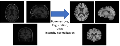
Figure E: We employed FreeSurfer Fischl (2012) for skull stripping, resizing, and intensity normalization of NACC dataset’s MRI volumes.

Additionally, we employed FreeSurfer Fischl (2012) for skull stripping, resizing, and intensity normalization of the MRI data, as illustrated in Fig. E. After FreeSurfer’s processing, each voxel is with dimensions of 182$\times$218$\times$182 voxels.

F Selecting Model for PE Tabular Classification

ElasticNet Zou and Hastie (2005), known for combining ridge and lasso regression features, was previously used for tabular data classification in the PE dataset Zhou et al. (2021). In our paper, the prediction is given by

$$\hat{y}=f_{\rm{a}}(\boldsymbol{\beta}^{\top}\boldsymbol{x}_{\rm{t}}+\beta_{0})$$ (16)

where each tabular data vector is denoted as a feature vector $\boldsymbol{x}_{\rm{t}}$ and the objective is to predict the class label by output $\hat{y}$. $\boldsymbol{\beta}$ is the vector of coefficients and $\beta_{0}$ is the intercept. The function $f_{\rm{a}}(\cdot)$ represents the activation function, mapping the linear combination to a class probability.

The coefficients $\boldsymbol{\beta}$ and $\beta_{0}$ are derived via ElasticNet regularization:

$$\min_{\boldsymbol{\beta}}\frac{1}{N}\sum_{n=1}^{N}\mathcal{L}(y_{n},\hat{y}_{n})+\lambda\left[(1-\alpha)\frac{1}{2}\|\boldsymbol{\beta}\|_{2}^{2}+\alpha\|\boldsymbol{\beta}\|_{1}\right],$$ (17)

where $\mathcal{L}$ is the loss function, $N$ is the number of instances, $\lambda$ the regularization weight, and $\alpha$ balances L1 and L2 penalties, facilitating feature selection and robustness in high-dimensional spaces.

ElasticNet demonstrated good performance (ACC=0.837) as reported in Zhou et al. Zhou et al. (2021) when all 1,505 attributes of the PE dataset’s tabular data were utilized. As stated in the paper, this high accuracy can be attributed to the inclusion of two attributes directly related to PE: “DISEASES OF PULMONARY CIRCULATION: frequency” and “DISEASES OF PULMONARY CIRCULATION: presence.” Our analysis revealed that if these two attributes are not 0, PE is positive. Consequently, to avoid bias, we decided to exclude these two attributes from our analysis.

Given the advancements in machine learning since ElasticNet’s introduction in 2005, we explored newer models to evaluate their effectiveness. This included the deep learning-based ResNet Jian et al. (2016), known for its deep network capabilities through skip connections; and the Tabular Transformer Gorishniy et al. (2021), which adapts the transformer architecture for structured data.

Our analysis shown in Table 5 in the paper, indicated that the Tabular Transformer outperformed other models, including ElasticNet and ResNet, in classifying the PE dataset. Consequently, we chose the Tabular Transformer as our baseline model due to its superior performance in handling complex tabular data.

G Additional Grad-CAM Results

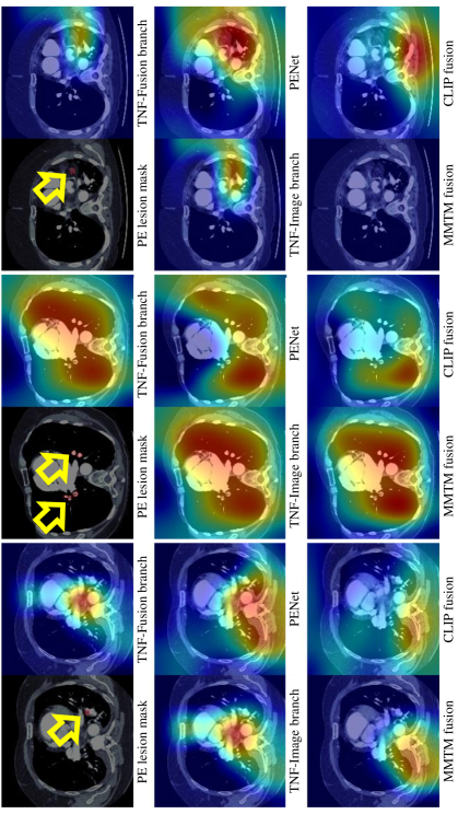
Figure F: More Grad-CAM heatmaps. Yellow arrows indicate PE lesions.

To demonstrate the superior performance of TNF-based models compared to others, additional Grad-CAM heatmaps are presented in Fig. F. We compared five types of Grad-CAM heatmaps: 1) The fusion branch of TNF. The model is shown in Fig. A (a); 2) The image branch of TNF; 3) PENet; 4) MMTM fusion model; The model’s structure is equivalent to the model in Fig. A (a) and only outputs fusion result; 5) Clip fusion model. Yellow arrows in Fig. F indicate PE lesions. In short, the highlighted parts of the TNF-based models are closer to the lesions.

References

- Acosta et al. [2022] Julián N Acosta, Guido J Falcone, Pranav Rajpurkar, and Eric J Topol. Multimodal biomedical AI. Nature Medicine, 28(9):1773–1784, 2022.
- Amal et al. [2022] Saeed Amal, Lida Safarnejad, Jesutofunmi A Omiye, Ilies Ghanzouri, John Hanson Cabot, and Elsie Gyang Ross. Use of multi-modal data and machine learning to improve cardiovascular disease care. Frontiers in Cardiovascular Medicine, 9:840262, 2022.
- Association [2023] Alzheimer’s Association. Medical tests for diagnosing Alzheimer’s. https://www.alz.org/alzheimers-dementia/diagnosis/medical_tests, 2023. Accessed: 2023-11-09.
- Baltrušaitis et al. [2018] Tadas Baltrušaitis, Chaitanya Ahuja, and Louis-Philippe Morency. Multimodal machine learning: A survey and taxonomy. IEEE transactions on pattern analysis and machine intelligence, 41(2):423–443, 2018.
- Beekly et al. [2004] Duane L Beekly, Erin M Ramos, Gerald van Belle, Woodrow Deitrich, Amber D Clark, Mary E Jacka, Walter A Kukull, et al. The national Alzheimer’s coordinating center (NACC) database: an Alzheimer disease database. Alzheimer Disease & Associated Disorders, 18(4):270–277, 2004.
- Beluch et al. [2018] William H Beluch, Tim Genewein, Andreas Nürnberger, and Jan M Köhler. The power of ensembles for active learning in image classification. In Proceedings of the IEEE conference on computer vision and pattern recognition, pages 9368–9377, 2018.
- Carreira et al. [2018] Joao Carreira, Eric Noland, Andras Banki-Horvath, Chloe Hillier, and Andrew Zisserman. A short note about Kinetics-600. arXiv preprint arXiv:1808.01340, 2018.
- Chicco et al. [2021] Davide Chicco, Niklas Tötsch, and Giuseppe Jurman. The Matthews correlation coefficient (MCC) is more reliable than balanced accuracy, bookmaker informedness, and markedness in two-class confusion matrix evaluation. BioData mining, 14(1):1–22, 2021.
- Dong et al. [2022] Yanni Dong, Quanwei Liu, Bo Du, and Liangpei Zhang. Weighted feature fusion of convolutional neural network and graph attention network for hyperspectral image classification. IEEE Transactions on Image Processing, 31:1559–1572, 2022.
- Fischl [2012] Bruce Fischl. Freesurfer. Neuroimage, 62(2):774–781, 2012.
- Funke et al. [2019] Isabel Funke, Sören Torge Mees, Jürgen Weitz, and Stefanie Speidel. Video-based surgical skill assessment using 3D convolutional neural networks. International journal of computer assisted radiology and surgery, 14:1217–1225, 2019.
- Gorishniy et al. [2021] Yury Gorishniy, Ivan Rubachev, Valentin Khrulkov, and Artem Babenko. Revisiting deep learning models for tabular data. In M. Ranzato, A. Beygelzimer, Y. Dauphin, P.S. Liang, and J. Wortman Vaughan, editors, Advances in Neural Information Processing Systems, volume 34, pages 18932–18943. Curran Associates, Inc., 2021.
- Hager et al. [2023] Paul Hager, Martin J. Menten, and Daniel Rueckert. Best of both worlds: Multimodal contrastive learning with tabular and imaging data. In Proceedings of the IEEE/CVF Conference on Computer Vision and Pattern Recognition (CVPR), pages 23924–23935, June 2023.
- Holste et al. [2021] Gregory Holste, Savannah C Partridge, Habib Rahbar, Debosmita Biswas, Christoph I Lee, and Adam M Alessio. End-to-end learning of fused image and non-image features for improved breast cancer classification from MRI. In Proceedings of the IEEE/CVF International Conference on Computer Vision, pages 3294–3303, 2021.
- Holste et al. [2023] Gregory Holste, Douwe van der Wal, Hans Pinckaers, Rikiya Yamashita, Akinori Mitani, and Andre Esteva. Improved multimodal fusion for small datasets with auxiliary supervision. arXiv preprint arXiv:2304.00379, 2023.
- Huang et al. [2020] Shih-Cheng Huang, Tanay Kothari, Imon Banerjee, Chris Chute, Robyn L Ball, Norah Borus, Andrew Huang, Bhavik N Patel, Pranav Rajpurkar, Jeremy Irvin, et al. PENet—a scalable deep-learning model for automated diagnosis of pulmonary embolism using volumetric CT imaging. NPJ digital medicine, 3(1):61, 2020.
- Jian et al. [2016] S Jian, H Kaiming, R Shaoqing, and Z Xiangyu. Deep residual learning for image recognition. In IEEE Conference on Computer Vision & Pattern Recognition, pages 770–778, 2016.
- Joze et al. [2020] Hamid Reza Vaezi Joze, Amirreza Shaban, Michael L Iuzzolino, and Kazuhito Koishida. MMTM: Multimodal transfer module for CNN fusion. In Proceedings of the IEEE/CVF conference on computer vision and pattern recognition, pages 13289–13299, 2020.
- Kumar et al. [2016] Ashnil Kumar, Jinman Kim, David Lyndon, Michael Fulham, and Dagan Feng. An ensemble of fine-tuned convolutional neural networks for medical image classification. IEEE journal of biomedical and health informatics, 21(1):31–40, 2016.
- Li and Li [2020] Pei Li and Xinde Li. Multimodal fusion with co-attention mechanism. In 2020 IEEE 23rd International Conference on Information Fusion (FUSION), pages 1–8. IEEE, 2020.
- Loshchilov and Hutter [2018] Ilya Loshchilov and Frank Hutter. Decoupled weight decay regularization. In International Conference on Learning Representations, 2018.
- Lundberg and Lee [2017] Scott M Lundberg and Su-In Lee. A unified approach to interpreting model predictions. In I. Guyon, U. V. Luxburg, S. Bengio, H. Wallach, R. Fergus, S. Vishwanathan, and R. Garnett, editors, Advances in Neural Information Processing Systems 30, pages 4765–4774. Curran Associates, Inc., 2017.
- Mobadersany et al. [2018] Pooya Mobadersany, Safoora Yousefi, Mohamed Amgad, David A Gutman, Jill S Barnholtz-Sloan, José E Velázquez Vega, Daniel J Brat, and Lee AD Cooper. Predicting cancer outcomes from histology and genomics using convolutional networks. Proceedings of the National Academy of Sciences, 115(13):E2970–E2979, 2018.
- Pagad et al. [2022] Naveen S Pagad, Khalid K Almuzaini, Manish Maheshwari, Durgaprasad Gangodkar, Piyush Shukla, Musah Alhassan, et al. Clinical text data categorization and feature extraction using medical-fissure algorithm and Neg-Seq algorithm. Computational Intelligence and Neuroscience, 2022(5759521), 2022.
- Panda et al. [2021] Rameswar Panda, Chun-Fu Richard Chen, Quanfu Fan, Ximeng Sun, Kate Saenko, Aude Oliva, and Rogerio Feris. AdaMML: Adaptive multi-modal learning for efficient video recognition. In Proceedings of the IEEE/CVF international conference on computer vision, pages 7576–7585, 2021.
- Pei et al. [2023] Xiangdong Pei, Ke Zuo, Yuan Li, and Zhengbin Pang. A review of the application of multi-modal deep learning in medicine: bibliometrics and future directions. International Journal of Computational Intelligence Systems, 16(1):44, 2023.
- Qiu et al. [2022] Shangran Qiu, Matthew I Miller, Prajakta S Joshi, Joyce C Lee, Chonghua Xue, Yunruo Ni, Yuwei Wang, Ileana De Anda-Duran, Phillip H Hwang, Justin A Cramer, et al. Multimodal deep learning for Alzheimer’s disease dementia assessment. Nature communications, 13(1):3404, 2022.
- Rokach [2010] Lior Rokach. Pattern classification using ensemble methods, volume 75. World Scientific, 2010.
- Selvaraju et al. [2017] Ramprasaath R Selvaraju, Michael Cogswell, Abhishek Das, Ramakrishna Vedantam, Devi Parikh, and Dhruv Batra. Grad-CAM: Visual explanations from deep networks via gradient-based localization. In Proceedings of the IEEE international conference on computer vision, pages 618–626, 2017.
- Shaik et al. [2023] Thanveer Shaik, Xiaohui Tao, Lin Li, Haoran Xie, and Juan D Velásquez. A survey of multimodal information fusion for smart healthcare: Mapping the journey from data to wisdom. Information Fusion, page 102040, 2023.
- Shrikumar et al. [2017] Avanti Shrikumar, Peyton Greenside, and Anshul Kundaje. Learning important features through propagating activation differences. In International conference on machine learning, pages 3145–3153. PMLR, 2017.
- Singh et al. [2020] Satya P Singh, Lipo Wang, Sukrit Gupta, Haveesh Goli, Parasuraman Padmanabhan, and Balázs Gulyás. 3D deep learning on medical images: a review. Sensors, 20(18):5097, 2020.
- Su et al. [2020] Chang Su, Zhenxing Xu, Jyotishman Pathak, and Fei Wang. Deep learning in mental health outcome research: a scoping review. Translational Psychiatry, 10(1):116, 2020.
- Taleb et al. [2021] Aiham Taleb, Christoph Lippert, Tassilo Klein, and Moin Nabi. Multimodal self-supervised learning for medical image analysis. In International conference on information processing in medical imaging, pages 661–673. Springer, 2021.
- Uppal et al. [2021] Shagun Uppal, Sarthak Bhagat, Devamanyu Hazarika, Navonil Majumder, Soujanya Poria, Roger Zimmermann, and Amir Zadeh. Multimodal research in vision and language: A review of current and emerging trends. Information Fusion, 77, 2021.
- Vaswani et al. [2017] Ashish Vaswani, Noam Shazeer, Niki Parmar, Jakob Uszkoreit, Llion Jones, Aidan N Gomez, Łukasz Kaiser, and Illia Polosukhin. Attention is all you need. Advances in neural information processing systems, 30, 2017.
- Wang and Zuo [2022] Lei Wang and Keqiang Zuo. Medical data classification assisted by machine learning strategy. Journal of Artificial Intelligence Research, 2022(9699612), 2022.
- Wang et al. [2022] Yikai Wang, Xinghao Chen, Lele Cao, Wenbing Huang, Fuchun Sun, and Yunhe Wang. Multimodal token fusion for vision transformers. In Proceedings of the IEEE/CVF Conference on Computer Vision and Pattern Recognition, pages 12186–12195, 2022.
- Xiao et al. [2020] Yi Xiao, Felipe Codevilla, Akhil Gurram, Onay Urfalioglu, and Antonio M López. Multimodal end-to-end autonomous driving. IEEE Transactions on Intelligent Transportation Systems, 23(1):537–547, 2020.
- Yao et al. [2017] Jiawen Yao, Xinliang Zhu, Feiyun Zhu, and Junzhou Huang. Deep correlational learning for survival prediction from multi-modality data. In International Conference on Medical Image Computing and Computer-Assisted Intervention, pages 406–414. Springer, 2017.
- Yap et al. [2018] Jordan Yap, William Yolland, and Philipp Tschandl. Multimodal skin lesion classification using deep learning. Experimental dermatology, 27(11):1261–1267, 2018.
- Yoo et al. [2019] Youngjin Yoo, Lisa YW Tang, David KB Li, Luanne Metz, Shannon Kolind, Anthony L Traboulsee, and Roger C Tam. Deep learning of brain lesion patterns and user-defined clinical and MRI features for predicting conversion to multiple sclerosis from clinically isolated syndrome. Computer Methods in Biomechanics and Biomedical Engineering: Imaging & Visualization, 7(3):250–259, 2019.
- Zhang et al. [2021] Mengmeng Zhang, Wei Li, Ran Tao, Hengchao Li, and Qian Du. Information fusion for classification of hyperspectral and LiDAR data using IP-CNN. IEEE Transactions on Geoscience and Remote Sensing, 60:1–12, 2021.
- Zhou et al. [2021] Yuyin Zhou, Shih-Cheng Huang, Jason Alan Fries, Alaa Youssef, Timothy J Amrhein, Marcello Chang, Imon Banerjee, Daniel Rubin, Lei Xing, Nigam Shah, et al. Radfusion: Benchmarking performance and fairness for multimodal pulmonary embolism detection from CT and EHR. arXiv preprint arXiv:2111.11665, 2021.
- Zou and Hastie [2005] Hui Zou and Trevor Hastie. Regularization and variable selection via the elastic net. Journal of the Royal Statistical Society Series B: Statistical Methodology, 67(2):301–320, 2005.