Isospin-forbidden electric dipole transition of the 9.64 MeV state of ¹²C

Abstract

The electric dipole transition of the 3^- state at 9.64 MeV of ¹²C to the 2⁺ state at 4.44 MeV is speculated to play a key role in the triple-$\alpha$ reaction at high temperatures. A theoretical prediction of its transition width is a challenge to nuclear theory because it belongs to a class of isospin-forbidden transitions. We extend a microscopic 3$\alpha$ cluster-model to include isospin 1 impurity components, and take into account both isovector and isoscalar electirc dipole operators. Several sets of $2^{+}$ and $3^{-}$ wave functions are generated by solving a radius-constrained equation of motion with the stochastic variational method, resulting in reproducing very well the electric quadrupole and octupole transition probabilities to the ground state. The electric dipole transition width is found to be 7–31 meV, 16 meV on the average, and more than half of the width is contributed by the isospin mixing of $\alpha$ particles.

I Introduction

It is well-known that the triple-$\alpha$ reaction is a key reaction to produce the elements heavier than ¹²C. At low temperatures, it occurs through the $0^{+}$ Hoyle state at 7.65 MeV [1, 2]. Its importance is numerically confirmed [3, 4], in reasonable agreement with the $R$-matrix prediction [5] at $T<0.1$ GK.

At higher temperatures, $T>2$ GK, relevant to supernovae and X-ray bursts, the triple-$\alpha$ reaction via the $3^{-}$ state at 9.64 MeV of ¹²C is presumed to play an important role. To estimate its impact, the radiative decay of the $3^{-}$ state relative to its total width has been measured [6, 7], and an upper limit of $\Gamma_{\rm rad}/\Gamma_{\rm total}<4.1\times 10^{-7}$ was deduced [8, 9]. Recently, two independent experiments have attempted to update the ratio, indicating $\Gamma_{\rm rad}/\Gamma_{\rm total}=1.3^{+1.2}_{-1.1}\times 10^{-6}$ [10] and $6.4\pm 5.1\times 10^{-5}$ [11], respectively. Both of them appear to be much larger than the previous upper limit, although the substantial uncertainties make it difficult to determine whether or not the $3^{-}$ state really contributes to the synthesis of ¹²C at high temperatures. Hence, a theoretical evaluation is necessary and important.

It should be noted that the radiative decay width from the $3^{-}$ state to the first $2^{+}$ state is the primary source of the uncertainty, because the total width ($\Gamma_{\rm total}=46\pm 3$ keV [9] or $34\pm 5$ keV [8]) is well constrained [12] and the electric octupole ($E3$) decay width to the ground state ($0.31\pm 0.04$ meV [13]) is rather small. A width due to the magnetic quadrupole transition is also expected to be small. The radiative decay from the $3^{-}$ state to the $2^{+}$ state should therefore be dominated by an electric dipole ($E1$) transition. The decay is, however, hindered in the long-wavelength approximation, because both states are considered to be good isospin zero states. It is thus necessary to go beyond the long-wavelength approximation and furthermore to take into account the breaking of isospin symmetry, which is a challenging task to nuclear theory.

The purpose of the present study is to estimate the $E1$ decay rate by assuming that the relevant states are all described well by a microscopic 3$\alpha$ cluster-model. Many calculations have been performed in the cluster model using effective two-nucleon central forces. See, e.g., Refs. [14, 15, 16]. The binding energy, the spectrum of ¹²C, and some other observables are reasonably well reproduced. However, describing the $\alpha$ cluster with $\phi_{\alpha}^{(0)}=(0s)^{4}$ harmonic-oscillator configuration fails in calculating the $E1$ transition probability because all the 3$\alpha$ configurations are isospin zero states. Let us clarify the point of the present study. Up to the leading-order term beyond the long-wavelength approximation, the $E1$ operator acting on an $A$-nucleon system reads as [17]

$$E_{1\mu}=E_{1\mu}({\rm IV})+E_{1\mu}({\rm IS}),$$

$$E_{1\mu}({\rm IV})=e\sum_{i\in{\rm proton}}{\cal Y}_{1\mu}({\bm{r}}_{i}-{\bm{R}}),$$

$$E_{1\mu}({\rm IS})=-e\frac{k^{2}}{10}\sum_{i=1}^{A}({\bm{r}}_{i}-{\bm{R}})^{2}{\cal Y}_{1\mu}({\bm{r}}_{i}-{\bm{R}})$$

$$+\frac{e\hbar k}{8m_{p}c}\frac{2i}{\hbar}\sum_{i=1}^{A}{\cal Y}_{1\mu}({\bm{r}}_{i}-{\bm{R}})\,({\bm{r}}_{i}-{\bm{R}})\cdot({\bm{p}}_{i}-\textstyle{\frac{1}{A}}{\bm{P}}).$$ (1)

Here, $\bm{r}_{i}$ and $\bm{p_{i}}$ are respectively the position coordinate and the momentum of the $i$th nucleon, $k$ the wave number of the $E1$ transition, $m_{p}$ the proton mass, $\bm{R}$ and $\bm{P}$ are respectively the center-of-mass coordinate and the total momentum, and ${\cal Y}_{lm}(\bm{r})$ is the solid spherical harmonics

$${\cal Y}_{lm}(\bm{r})=r^{l}Y_{lm}(\hat{\bm{r}}),$$ (2)

where $\hat{\bm{r}}$ stands for the polar and azimuthal angles of $\bm{r}$. $E_{1\mu}({\rm IV})$ is isovector and the leading term of the long-wavelength approximation. It has no contribution to an isospin zero nucleus. Therefore, we have to evaluate the contribution of the isoscalar term, $E_{1\mu}({\rm IS})$, to the $E1$ matrix element, provided that we use the $3\alpha$ cluster-model for ¹²C. Though $E_{1\mu}({\rm IS})$ further contains a spin-dependent term [17], we ignore it because ¹²C is described by the $3\alpha$ cluster-model with zero total spin. Another variant of expression for the isoscalar $E1$ operator is also discussed in Ref. [17].

There is the possibility, however, that $E_{1\mu}({\rm IV})$ receives non-vanishing contribution in so far as the relevant states of ¹²C contain isospin impurity components. We take into account the isospin mixing assuming that the $\alpha$ particle contains a small component of isospin 1 impurity configuration, $\phi^{(1)}_{\alpha}$,

$$\phi_{\alpha}=\sqrt{1-\epsilon^{2}}\phi_{\alpha}^{(0)}+\epsilon\phi^{(1)}_{\alpha},$$ (3)

as described in Ref. [18]. Contrary to $E_{1\mu}({\rm IV})$, $E_{1\mu}({\rm IS})$ gives nonzero contributions between the main isospin zero components of ¹²C. Both contributions of the isovector and isoscalar terms may compete with each other.

Three states of ¹²C play a main role in the present study: the ground state, the 2⁺ state at $E_{\rm x}\,=$ 4.44 MeV, and the 3^- state at $E_{\rm x}\,=$ 9.64 MeV. Since the $E1$ transition matrix element is sensitive to the sizes of the relevant states, we obtain the wave functions of those states by taking into account not only the energies but also other physical observables sensitive to the sizes, that is, the point proton radius of the ground state, the electric quadrupole ($E2$) transition probability, $B(E2)$, from the $2^{+}$ state to the ground state, and the $E3$ transition probability, $B(E3)$, of the $3^{-}$ state to the ground state.

Section II describes a way of constructing the relevant states and then explains how to include the isospin impurity components in evaluating the $E1$ transition matrix element. Section III presents results of calculation for the ground state, the $2^{+}$ state, and the $3^{-}$ state and discusses the isospin-forbidden $E1$ transition probability. A brief summary is drawn in Sec. IV.

II Formulation

As is well-known, it is very hard to reproduce the binding energy and the excitation energies of the three states of ¹²C with effective nuclear forces such as Volkov [19] and Minnesota [20] potentials. Instead of minimizing the Hamiltonian expectation value, we constrain the size or radius of the system and study the energy as a function of the radius. This is reasonable because the size of the system is expected to play a vital role in the present study. We introduce a combination of operators, the Hamiltonian, $H$, and the mean square radius, $R^{2}$,

$$S(\lambda)=H+\lambda R^{2}.$$ (4)

Here, $\lambda$ is a parameter. Given $\lambda$, we search for such a solution that the expectation value of $S(\lambda)$ becomes a minimum, denoted by $\left<S\right>_{\lambda}$. Using the obtained wave function, we evaluate the expectation values, $\left<H\right>$ and $\left<R^{2}\right>$. In this way we can study both energy and size of the relevant state at the same time as a function of $\lambda$.

Except for the point proton radius of the ground state, there is no direct information on the sizes of the 2⁺ state and the 3^- resonance state. As noted above, however, we can make use of the $B(E2)$ value of the 2⁺ state and the $B(E3)$ value of the 3^- state to determine $\lambda$. We take non-negative $\lambda$ in the present study. A negative value of $\lambda$ may play a role when ¹²C extends to strongly deformed configurations or fragments into $\alpha+2\alpha$ or $\alpha+\alpha+\alpha$ system. In what follows, $\lambda$ is denoted by $\lambda_{L}$, where $L$ is the total angular momentum of ¹²C.

The minimization of $S(\lambda_{L})$ is performed by taking a combination of correlated Gaussian (CG) bases $\Phi_{LM}$ [21]:

$$\Psi_{LM}=\sum_{k=1}^{K}C(k)\Phi_{LM}(k),$$

$$\Phi_{LM}(k)={\cal A}\Big{\{}{\cal Y}_{LM}(\widetilde{u_{k}}\bm{x})e^{-\frac{1}{2}\tilde{\bm{x}}A_{k}\bm{x}}\prod_{i=1}^{3}\phi^{(0)}_{\alpha}(i)\Big{\}},$$ (5)

where ${\cal A}$ is the antisymmetrizer of 12 nucleons. The coordinate $\bm{x}$ is a 2-dimensional column vector specifying the relative coordinates of 3 $\alpha$-particles: ${\bm{x}}_{1}={\bm{R}}_{1}-{\bm{R}}_{2},\ {\bm{x}}_{2}=\frac{1}{2}({\bm{R}}_{1}+{\bm{R}}_{2})-{\bm{R}}_{3}$, where ${\bm{R}}_{i}$ stands for the center-of-mass coordinate of the $i$th $\alpha$-particle. The CG basis $\Phi_{LM}(k)$ is characterized by variational parameters, $u_{k}$ and $A_{k}$: $u_{k}$ is a column vector of 2-dimension, and $A_{k}$ is a $2\times 2$ real, symmetric, positive-definite matrix. The tilde symbol $\tilde{\ }$ stands for the transpose of a column vector, that is, $\widetilde{u_{k}}\bm{x}=u_{k}(1)\bm{x}_{1}+u_{k}(2)\bm{x}_{2},\,\tilde{\bm{x}}A_{k}\bm{x}=A_{k}(1,1)\bm{x}_{1}^{\,2}+2A_{k}(1,2)\bm{x}_{1}\cdot\bm{x}_{2}+A_{k}(2,2)\bm{x}_{2}^{\,2}$. No generality is lost by assuming $\widetilde{u_{k}}u_{k}=1$. Each CG basis thus contains 3 parameters for $L=0$ and 4 parameters for $L=2,3$. The matrix $A_{k}$ is conveniently defined through three relative distance parameters, $(d_{k}(12),d_{k}(13),d_{k}(23))$, by [22, 23]

$$\tilde{\bm{x}}A_{k}\bm{x}=\sum_{j>i=1}^{3}\Big{(}\frac{{\bm{R}}_{i}-{\bm{R}}_{j}}{d_{k}(ij)}\Big{)}^{\,2}.$$ (6)

We note the following in choosing the set $\{d_{k}(ij)\}$: The root-mean-square (rms) radius of the center-of-masses of 3 $\alpha$-particles is defined by $\sqrt{\frac{1}{3}\sum_{i=1}^{3}({\bm{R}}_{i}-{\bm{R}})^{2}}=\frac{1}{3}\sqrt{\sum_{j>i=1}^{3}({\bm{R}}_{i}-{\bm{R}}_{j})^{2}}$, where ${\bm{R}}=\frac{1}{3}\sum_{i=1}^{3}{\bm{R}}_{i}$. Therefore, $\bar{D}_{k}=\frac{1}{3}\sqrt{\sum_{j>i=1}^{3}d_{k}(ij)^{2}}$ controls the global size of the 3$\alpha$ system. We choose $\{d_{k}(ij)\}$ to make $\bar{D}_{k}$ cover sufficiently large values.

Calculation of all the needed matrix elements can be done as explained in Ref. [18]. It is worthwhile to note that the angular-momentum projection is carried out analytically, which guarantees an accurate evaluation of all the matrix elements. This accuracy is a vitally important ingredient to make a stochastic search of the basis set possible and practical. Both $u_{k}$ and $A_{k}$ serve to control the partial-wave contents among $\alpha$-particles. The parameters, $u_{k}$ and $A_{k}$, are determined by the stochastic variational method [21, 23]. The previous calculation for the $0^{+}$ case suggests that the basis dimension $K$ could be a small value [24]: $K$ is set to 7 for the 0⁺ state and to 20 for the $2^{+}$ and $3^{-}$ states. The basis determination consists of (i) a trial and error search of the basis set up to $K$ dimension, followed by (ii) a refining search that replaces the already selected base with a new candidate base if the latter decreases the expectation value of $S(\lambda_{L})$. Random bases tested in each step of (i) and (ii) are typically 15–20. A refinement cycle is repeated more than ten times. It should be stressed that we have to obtain a well-converged solution to draw a reliable $B(E1)$ value because it could be very sensitive to the details of the relevant wave functions.

The wave function of $\alpha$-particle $\phi^{(0)}_{\alpha}$ is constructed from the $(0s)^{4}$ harmonic-oscillator configuration with its center-of-mass motion excluded. Its single-particle orbit is a Gaussian function, ${\rm exp}(-\frac{\beta}{2}r^{2})$, with $\beta=0.52$ fm^-2. Since $\epsilon$ is on the order of $10^{-3}$ [18], evaluating the matrix elements of $S(\lambda_{L})$ is carried out with $\phi^{(0)}_{\alpha}$ as defined in Eq. (5) but not with $\phi_{\alpha}$ of Eq. (3). The impurity component $\phi^{(1)}_{\alpha}$ is normalized and has the same quantum numbers as $\phi^{(0)}_{\alpha}$ except for the isospin. The spatial part of $\phi^{(1)}_{\alpha}$ is constructed from a 2$\hbar\omega$ excited shell-model configuration with its spurious center-of-mass motion being excluded [18]. Once $\Psi_{LM}$ is obtained, it is reasonable to define a 3$\alpha$ wave function with isospin mixing, $\Psi^{\prime}_{LM}$, by replacing $\phi^{(0)}_{\alpha}(i)$ with $\phi_{\alpha}(i)$ in Eq. (5). Since $\epsilon$ is sufficiently small, $\Psi^{\prime}_{LM}$ can be very well approximated up to the first order in $\epsilon$ as follows:

$$\Psi^{\prime}_{LM} =(1-\epsilon^{2})^{\frac{3}{2}}\Psi_{LM}+\epsilon(1-\epsilon^{2})\sum_{i=1}^{3}\Psi_{LM}(i)+\cdots$$

$$\approx\Psi_{LM}+\epsilon\sum_{i=1}^{3}\Psi_{LM}(i).$$ (7)

Here, $\Psi_{LM}(i)$ is defined by replacing $\phi^{(0)}_{\alpha}(i)$ by $\phi^{(1)}_{\alpha}(i)$ in Eq. (5), whereas the rest of the $\alpha$-particle wave functions is unchanged, thus $\Psi_{LM}(i)$ has isospin 1. Since the $E1$ operator consists of the isovector and isoscalar terms, Eq. (1), the $E1$ matrix element read as

$$\langle\Psi^{\prime}_{L^{\prime}M^{\prime}}|E_{1\mu}({\rm IV})+E_{1\mu}({\rm IS})|\Psi^{\prime}_{LM}\rangle$$

$$\ \ \ \approx\langle\Psi_{L^{\prime}M^{\prime}}|E_{1\mu}({\rm IS})|\Psi_{LM}\rangle$$

$$\ \ \ +\epsilon\sum_{i=1}^{3}\Big{\{}\langle\Psi_{L^{\prime}M^{\prime}}|E_{1\mu}({\rm IV})|\Psi_{LM}(i)\rangle\Big{.}$$

. $$\ \ \ \ \ \ \ \ \ \ \ \ +\langle\Psi_{L^{\prime}M^{\prime}}(i)|E_{1\mu}({\rm IV})|\Psi_{LM}\rangle\Big{\}}.$$ (8)

Here, the first term is the contribution of the isoscalar $E1$ operator between the main components of the wave functions with isospin 0, while the second terms are the contributions of the isovector $E1$ operator including the small components of the 3$\alpha$ wave function with isospin 1 either in the ket or in the bra.

It should be noted that the transition matrix element $\langle\Psi_{L^{\prime}M^{\prime}}|E_{1\mu}({\rm IV})|\Psi_{LM}(i)\rangle$ can be nonzero only when $E_{1\mu}({\rm IV})|\Psi_{LM}(i)\rangle$ contains the same spin-isospin functions as that of $\Psi_{L^{\prime}M^{\prime}}$, that is, a product of three totally antisymmetric spin-isospin functions. As was done in Ref. [18], it is convenient to decompose $E_{1\mu}({\rm IV})$ into $E_{1\mu}({\rm IV})=\sum_{p=1}^{3}E_{1\mu}({\rm IV},p)$ with

$$E_{1\mu}({\rm IV},p)=e\sum_{q=1}^{4}\Big{(}\frac{1}{2}-t_{3}(p_{q})\Big{)}{\cal Y}_{1\mu}({\bm{r}}_{p_{q}}-{\bm{R}}_{p}),$$ (9)

where $t_{3}$ is the $z$ component of the nucleon isospin, $p_{q}$ is introduced to denote the nucleon label of the $p$th $\alpha$-particle, and its center-of-mass coordinate is given by ${\bm{R}}_{p}=\frac{1}{4}\sum_{q=1}^{4}{\bm{r}}_{p_{q}}$. Only the $p=i$ term among three sums over $p$ satisfies the condition, leading to

$$\sum_{i=1}^{3}E_{1\mu}({\rm IV})|\Psi_{LM}(i)\rangle\rightarrow E_{1\mu}^{\rm eff}({\rm IS})|\Psi_{LM}\rangle,$$ (10)

where $E_{1\mu}^{\rm eff}({\rm IS})$ is an effective isoscalar $E1$ operator given by

$$E_{1\mu}^{\rm eff}({\rm IS})=-e\frac{2\beta}{3\sqrt{3}}\sum_{i=1}^{3}\sum_{j=1}^{4}({\bm{r}}_{i_{j}}-{\bm{R}}_{i})^{2}{\cal Y}_{1\mu}({\bm{r}}_{i_{j}}-{\bm{R}}_{i}).$$ (11)

Substituting Eq. (10) into Eq. (8) enables us to evaluate the $E1$ matrix element including the effect of the isospin mixing as follows:

$$\langle\Psi^{\prime}_{L^{\prime}M^{\prime}}|E_{1\mu}({\rm IV})+E_{1\mu}({\rm IS})|\Psi^{\prime}_{LM}\rangle$$

$$\approx\langle\Psi_{L^{\prime}M^{\prime}}|E_{1\mu}({\rm IS})|\Psi_{LM}\rangle+2\epsilon\langle\Psi_{L^{\prime}M^{\prime}}|E_{1\mu}^{\rm eff}({\rm IS})|\Psi_{LM}\rangle.$$ (12)

The effect of the isospin mixing is thus taken care of in the conventional $\alpha$ cluster-model. What is needed is to calculate the matrix elements of $E_{1\mu}^{\rm eff}({\rm IS})$. It is interesting to compare the matrix elements of different types of isoscalar operators for the $E1$ transition from the $3^{-}$ state to the $2^{+}$ state.

III Results of calculation

Table 1: Results for the $0^{+}$ ground state of ¹²C. $\left<S\right>_{\lambda_{0}}$ and $\left<H\right>$ are values from 3$\alpha$ threshold. The observed $0^{+}$ ground state is located at $-7.27$ MeV below $3\alpha$ threshold [8, 9], and the point rms radius is 2.33 fm [26].

$\lambda_{0}$		$\left<S\right>_{\lambda_{0}}$		$\left<H\right>$		$\sqrt{\left<R^{2}\right>}$
MeV $\cdot$ fm-2		MeV		MeV		fm
0.0		$-$6.008		$-$6.008		2.456
0.4		$-$3.642		$-$5.959		2.406
0.8		$-$1.318		$-$5.835		2.376
1.2		0.903		$-$5.717		2.349
1.6		3.148		$-$5.570		2.334
2.0		5.354		$-$5.356		2.314

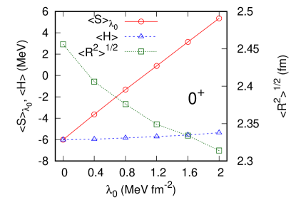
Figure 1: $\langle S\rangle_{\lambda_{0}}$, $\langle H\rangle$, and $\langle R^{2}\rangle$ as a function of $\lambda_{0}$. Thin lines are drawn for a guide to the eye.

We use Volkov No.1 two-nucleon central potential [19] with $m=0.59$, where $m$ is the parameter responsible for the Majorana exchange component. The value around $m=0.6$ is consistent with $\alpha\alpha$ scattering data [25]. The two-nucleon Coulomb potential is included. The energy of $\alpha$-particle turns out to be $-27.076$ MeV. Table 1 lists $L=0$ results of converged solutions as a function of $\lambda_{0}$. The case of $\lambda_{0}=0$ is the usual energy minimization. Interestingly, the variation of $\left<S\right>_{\lambda_{0}}$ as a function of $\lambda_{0}$ is quite large compared to those of $\left<H\right>$ and $\left<R^{2}\right>$. See also Fig.  1. As seen from the table, the $\lambda_{0}=0$ case predicts too large point rms radius for the ground state, which is about 2.33 fm [26]. Instead of this usual approach, we determine the $0^{+}$ ground state to be such a solution that reproduces the rms radius. The appropriate value of $\lambda_{0}$ is found to be about 1.6 MeV$\cdot$fm^-2. In what follows, we set up the ground state to be the solution obtained with $\lambda_{0}$= 1.6 MeV$\cdot$fm^-2. Note that the ground state energy is then $-5.57$ MeV from the 3$\alpha$ threshold, which is about 1.7 MeV too high compared to experiment.

Table 2 lists results of calculation for $L=2$. An appropriate value of $\lambda_{2}$ is determined by examining both the energy and the $B(E2)$ value to the ground state. The experimental values are respectively $-$2.84 MeV from the 3$\alpha$ threshold and $7.77\pm 0.43$ $e^{2}\,$fm⁴ [8, 9]. Figure 2 shows $\left<S\right>_{\lambda_{2}}$, $\left<H\right>$ and $B(E2)$ value as a function of $\lambda_{2}$. The case with $\lambda_{2}=0$ predicts that the $2^{+}$ energy is lower than experiment by about 0.6 MeV and the $B(E2)$ value is smaller than experiment. With $\lambda_{2}=0.2$–0.4 MeV$\cdot$fm^-2 both $\left<H\right>$ and $B(E2)$ become closer to the experimental values. The electric quadrupole moment $Q$ is calculated from $\sqrt{\frac{2}{35}}\langle\Psi_{2}\|Q_{\rm op}\|\Psi_{2}\rangle$ without assuming an intrinsic shape, where the double barred matrix element stands for a reduced matrix element. Theory appears to give slightly smaller value than $Q=6\pm 3$ $e\,$fm² [27].

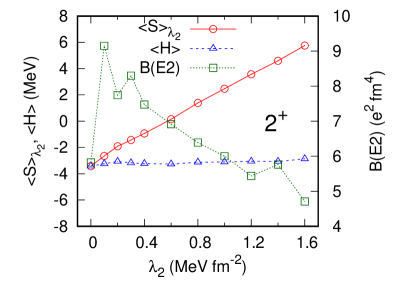
Figure 2: $\langle S\rangle_{\lambda_{2}}$, $\langle H\rangle$, and $B(E2)$ value as a function of $\lambda_{2}$. Thin lines are drawn for a guide to the eye.

Table 2: Results for the first excited $2^{+}$ state of ¹²C located at $-2.84$ MeV below 3$\alpha$ threshold [8, 9]. $Q$ is the electric quadrupole moment. The $B(E2)$ value extracted from the radiative width $\Gamma_{\gamma}$ [8, 9] is $7.77\pm 0.43$ $e^{2}\,$fm⁴.

$\lambda_{2}$		$\left<S\right>_{\lambda_{2}}$		$\left<H\right>$		$\sqrt{\left<R^{2}\right>}$		$B(E2)$		$Q$
MeV$\cdot$fm-2		MeV		MeV		fm		$e^{2}\,$fm4		$e\,$fm2
0.0		$-$3.418		$-$3.418		2.415		5.824		$-$1.856
0.1		$-$2.643		$-$3.238		2.438		9.150		1.441
0.2		$-$1.905		$-$3.068		2.411		7.744		$-$0.255
0.3		$-$1.431		$-$3.173		2.410		8.299		1.021
0.4		$-$0.929		$-$3.228		2.397		7.475		0.569
0.6		0.147		$-$3.261		2.383		6.914		1.410
0.8		1.390		$-$3.118		2.374		6.389		1.406
1.0		2.470		$-$3.101		2.360		6.000		1.251
1.2		3.570		$-$3.048		2.348		5.438		$-$0.032
1.4		4.596		$-$3.072		2.340		5.765		1.906
1.6		5.759		$-$2.866		2.322		4.710		$-$0.309

Table 3: Results for the $3^{-}$ resonance state of ¹²C located 2.37 MeV above $3\alpha$ threshold [8, 9]. The $B(E3)$ value extracted from the radiative width $\Gamma_{\gamma_{0}}$ [9] is $107\pm 14$ $e^{2}\,$fm⁶.

$\lambda_{3}$		$\left<S\right>_{\lambda_{3}}$		$\left<H\right>$		$\sqrt{\left<R^{2}\right>}$		$B(E3)$
MeV$\cdot$fm-2		MeV		MeV		fm		$e^{2}\,$fm6
0.4		4.703		1.626		2.773		378.7
0.6		6.186		1.775		2.711		636.9
0.7		6.900		1.840		2.689		6.331
0.8		7.621		1.928		2.668		22.14
0.9		8.333		2.004		2.652		78.16
1.0		9.034		2.093		2.635		126.9
1.1		9.722		2.169		2.620		104.4
1.2		10.403		2.248		2.607		92.99
1.3		11.078		2.327		2.595		95.50
1.4		11.754		2.405		2.584		85.51
1.5		12.416		2.474		2.575		44.61
1.6		13.067		2.544		2.565		44.18

Table 3 presents results of calculation for $L=3$. The $3^{-}$ state of ¹²C is by 2.37 MeV above $3\alpha$ threshold with the total width of $46\pm 3$ keV [9]. Its radiative decay width is less than 19 meV, and its partial width to the ground state decay is $(3.1\pm 0.4)\times 10^{-4}\,$eV [8, 9], indicating $B(E3:3^{-}\to 0^{+})=107\pm 14\ e^{2}\,$fm⁶. As the total width of the 3^- state is considerably small, it appears reasonable to treat the state as a bound state. The case of $\lambda_{3}=0$ cannot lead to a bound-state solution as expected: $\left<H\right>$ tends to be zero and $\sqrt{\left<R^{2}\right>}$ becomes larger and larger as the basis set reaches large distances. With positive $\lambda_{3}$, however, we obtain a positive-energy bound-solution as listed in Table 3. Figure 3 displays $\left<S\right>_{\lambda_{3}}$, $\left<H\right>$, and $B(E3)$ value as a function of $\lambda_{3}$. The observed excitation energy and the $B(E3)$ value are fairly well reproduced by taking $\lambda_{3}$ in the range of 1.0–1.4 MeV$\cdot$fm^-2.

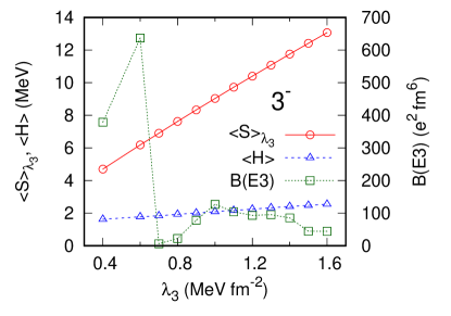
Figure 3: $\langle S\rangle_{\lambda_{3}}$, $\langle H\rangle$, and $B(E3)$ value as a function of $\lambda_{3}$. Thin lines are drawn for a guide to the eye.

Table 4: Radiation width of the $3^{-}$ resonance state of ¹²C to the 2⁺ state due to the electric dipole transition. The width, in units of meV, is calculated without the isospin mixing ($\epsilon=0$) or with the isospin mixing. The upper limit of the total radiation width of the $3^{-}$ resonance state is 19 meV [9]. Values in parentheses, in units of $10^{-2}e\,$fm, denote the $E1$ reduced matrix elements contributed by three kinds of isoscalar $E1$ operators. See Eq. (14).

$\lambda_{3}$		$\lambda_{2}$		$\quad\Gamma_{\rm rad}(3^{-}\to 2^{+})$
				$\epsilon=0$	$\epsilon=-0.0042$
1.0		0.2		8.58	26.0
					(7.41, $-$5.39, 1.50)
1.0		0.4		6.99	11.7
					(7.21, $-$5.38, $-$4.18)
1.1		0.2		3.34	9.49
					(5.01,$-$3.75, 0.86)
1.2		0.2		3.15	7.51
					(4.83, $-$3.61, 0.67)
1.2		0.4		2.44	19.2
					(4.70, $-$3.62, $-$4.10)
1.4		0.2		2.34	6.52
					(4.86, $-$3.81, 0.71)
1.4		0.4		2.21	30.7
					(4.85, $-$3.83, $-$4.84)

Using the $2^{+}$ and $3^{-}$ wave functions obtained above, we evaluate the $B(E1)$ value. The isospin mixing parameter $\epsilon$ is set to $-4.2\times 10^{-3}$ [18]. The radiation width due to the $E1$ transition is calculated from

$$\Gamma_{\rm rad}(3^{-}\to 2^{+})=1.473\times 10^{5}B(E1:3^{-}\to 2^{+}),$$ (13)

where $B(E1:3^{-}\to 2^{+})$ is given in units of $e^{2}{\,\rm fm}^{2}$ and $\Gamma_{\rm rad}$ is in units of meV. The ‘best’ wave functions obtained with $\lambda_{3}=1.1$ and $\lambda_{2}=0.2$ MeV$\cdot$fm^-2 predict the $B(E3)$ and $B(E2)$ values closest to the respective medians of the experimental values. In addition to this case, we test three $3^{-}$ states obtained with $\lambda_{3}=1.0,1.2$, and 1.4 MeV$\cdot$fm^-2 together with two $2^{+}$ states calculated from $\lambda_{2}=0.2$ and 0.4 MeV$\cdot$fm^-2. The $E1$ radiation width calculated from a combination of these wave functions is listed in Table 4. The largest width among 7 cases is 31 meV, the width from the ‘best’ combination is 9.5 meV, and the average of the widths is 16 meV consistently with the upper limit of $\Gamma_{\rm rad}<19$ meV [9]. The ratio of $\Gamma_{\rm rad}(3^{-}\to 2^{+})/\Gamma_{\rm total}(3^{-})$ with $\Gamma_{\rm total}(3^{-})=46\pm 3$ keV turns out to be 0.35$\times 10^{-6}$ on the average. The corresponding ratio of Ref. [10] is $1.3^{+1.2}_{-1.1}\times 10^{-6}$. The calculated theoretical ratio is within the error bars of that experiment, but it is much smaller than that quoted in Ref. [11]. If the isospin mixing of $\alpha$ particles is not taken into account, the $\Gamma_{\rm rad}(3^{-}\to 2^{+})$ value decreases to 4 meV on the average.

The average value of $\Gamma_{\rm rad}=16$ meV corresponds to $3.2\times 10^{-4}$ W.u. It is interesting to compare this value to the case of ¹⁶O where the $E1$ transition is isospin-forbidden and $\Gamma_{\rm rad}(E1)$ values are known. The $\Gamma_{\rm rad}(E1)$ values in Weisskopf units are $(3.5\pm 0.4)\times 10^{-4}$ for the $1^{-}$ state at 7.12 MeV and $(6.0\pm 0.9)\times 10^{-5}$ for the $1^{-}$ state at 9.63 MeV, respectively [28]. The value we obtain for ¹²C is in good correspondence with the ¹⁶O case. This indicates that the approach developed in this paper is sound and useful for evaluating the isospin-forbidden $E1$ transition strength.

Also shown in the table is the contribution of each of three different isoscalar operators to the $B(E1)$ value,

$$B(E1:3^{-}\to 2^{+})=\frac{1}{7}\Big{|}\sum_{i=1}^{3}\langle\Psi_{2}\|E1({\rm IS};i)\|\Psi_{3}\rangle\Big{|}^{2}.$$ (14)

Here, three kinds of isoscalar $E1$ operators are (i) the first term of $E_{1\mu}({\rm IS})$ in Eq. (1), (ii) the second term of $E_{1\mu}({\rm IS})$ in Eq. (1), and (iii) the effective isoscalar $E1$ operator, Eq. (11). The reduced matrix element of the first type is larger in its magnitude than that of the second type and they cancell each other. The isospin impurity term appears to increase the $B(E1)$ value in most cases, but its magnitude fluctuates depending on the choice of $\lambda_{2}$ and $\lambda_{3}$.

It is convenient to express the reduced matrix element as a product of a numerical constant, $CC(i)$, and an integral, ${\rm RME}(i)$, as follows:

$$\langle\Psi_{2}\|E1({\rm IS};i)\|\Psi_{3}\rangle=CC(i)\,{\rm RME}(i),$$ (15)

where

$$CC(1)=-\frac{k^{2}}{10},\quad CC(2)=\frac{\hbar k}{4m_{p}cR^{2}},\quad CC(3)=-\frac{4\beta\epsilon}{3\sqrt{3}},$$

$${\rm RME}(1)=e\,\langle r^{2}{\cal Y}_{1}(\bm{r})\rangle,\quad{\rm RME}(2)=e\,R^{2}\langle{\bm{r}}\cdot{\bm{\nabla}}{\cal Y}_{1}(\bm{r})\rangle,$$

$${\rm RME}(3)=e\,\langle r^{2}{\cal Y}_{1}(\bm{r})\rangle^{\prime}.$$ (16)

Here, $R$ is a radius introduced to make ${\rm RME}(2)$ have $e$ times length dimension, and the prime put for RME(3) is to stress that the operator involved there is not the same as that of RME(1). It is very likely that $|$RME(3)$|$ is smaller than $|$RME(1)$|$. The operators involved in RME(1) and RME(3) are both $r^{2}{\cal Y}_{1}(\bm{r})$ type, but their ranges are different. In RME(1) $\bm{r}$ denotes the distance vector of each nucleon from the center-of-mass of ¹²C, whereas it is the distance vector between the nucleon and the $\alpha$-particle to which the nucleon belongs. The latter is short-ranged and it appears that its matrix element depends on more detailed properties of the wave function.

The importance of these three terms apparently depends on the wave number $k$ as well as the maginitude of RME($i$). Note that $CC(3)$ is a constant determined by the property of the $\alpha$ particle, whereas the other two depend on the $E1$ transition energy, that is, the wave number $k$. With the use of $k=0.0264$  fm^-1, $\beta=0.52$  fm^-2, $\epsilon=-0.0042$, and $R=2.52$  fm, the relative ratio of $CC(i)$s’ is

$$CC(2)/CC(1) =-\frac{0.525}{R^{2}k}=-3.13,$$

$$CC(3)/CC(1) =-\frac{0.0168}{k^{2}}=-24.1.$$ (17)

These ratios qualitatively explain the results of Table 4. With decreasing $k$, the terms with $i=2,3$ become more important.

IV Summary

We have studied the electric dipole transition of the 9.64 MeV 3^- state of ¹²C to the 4.44 MeV 2⁺ state. The transition belongs to a class of isospin-forbidden transitions, demanding a study beyond the usual long-wavelength approximation of the electric transition operators. We have employed a microscopic $3\alpha$ cluster-model to generate the ground state, the $2^{+}$ state, and the $3^{-}$ state. In determining the wave functions of those states, however, we have attempted to reproduce experimental observables sensitive to their sizes in addition to their energies.

We have used the stochastic variational method to determine the wave functions. Among several combinations of $2^{+}$ and $3^{-}$ wave functions obtained within the accuracy of the experimental observables, we have selected several candidates to estimate the electric dipole transition probability. We have taken into account not only the next-order term beyond the long-wavelength approximation but also isospin mixings in both states of ¹²C. The resulting $\Gamma_{\rm rad}(3^{-}\to 2^{+})$ value ranges 7 to 31 meV, the average of those values is 16 meV, and more than half of the width is contributed by the isospin mixing of $\alpha$ particles. The $\Gamma_{\rm rad}$ value obtained here is considerably larger than 2 meV that was assumed in Ref. [5].

This study has been motivated by a question of whether or not the 9.64 MeV state plays an important role to triple-$\alpha$ reactions at high temperatures. There is no experimental information at present to test the $\Gamma_{\rm rad}$ value reported here. However, it is well-known that the $E1$ transition of the 7.12 MeV $1^{-}$ state of ¹⁶O to its ground state plays a crucially important role in ¹²C$(\alpha,\gamma)^{16}$O radiative capture reactions near the Gamow window. The $E1$ transition in that case is again isospin-forbidden. A study similar to the present one will be interesting and useful. Furthermore, such calculation can directly be compared to the observed radiation width.

- [1] E. E. Salpeter, Astrophys. J. 115, 326 (1952).
- [2] F. Hoyle, Astrophys. J., Suppl. 1, 121 (1954).
- [3] S. Ishikawa, Phys. Rev. C 87, 055804 (2013).
- [4] H. Suno, Y. Suzuki, and P. Descouvemont, Phys. Rev. C 94, 054607 (2016).
- [5] C. Angulo, M. Arnould, M. Rayet, P. Descouvemont, D. Baye, C. Leclercq-Willain, A. Coc, S. Barhoumi, P. Aguer, C. Rolfs, R. Kunz, J. W. Hammer, A. Mayer, T. Paradellis, S. Kossionides, C. Chronidou, K. Spyrou, S. Degl’Innocenti, G. Fiorentini, B. Ricci, S. Zavatarelli, C. Providencia, H. Wolters, J. Soares, C. Grama, J. Rahighi, A. Shotter, and M. L. Rachti, Nucl. Phys. A 656, 3 (1999).
- [6] H. Crannell, T. A. Griffy, L. R. Suezle, and M. R. Yearian, Nucl. Phys. A 90, 152 (1967).
- [7] D. Chamberlin, D. Bodansky, W. W. Jacobs, and D. L. Oberg, Phys. Rev. C 10, 909 (1974).
- [8] F. Ajzenberg-Selove, Nucl. Phys. A 506, 1 (1990).
- [9] J. H. Kelley, J. E. Purcell, and C. G. Sheu, Nucl. Phys. A 968, 71 (2017).
- [10] M. Tsumura, T. Kawabata, Y. Takahashi, S. Adachi, H. Akimune, S. Ashikaga, T. Baba, Y. Fujikawa, H. Fujimura, H. Fujioka, T. Furuno, T. Hashimoto, T. Harada, M. Ichikawa, K. Inaba, Y. Ishii, N. Itagaki, M. Itoh, C. Iwamoto, N. Kobayashi, A. Koshikawa, S. Kubono, Y. Maeda, Y. Matsuda, S. Matsumoto, K. Miki, T. Morimoto, M. Murata, T. Nanamura, I. Ou, S. Sakaguchi, A. Sakaue, M. Sferrazza, K.N. Suzuki, T. Takeda, A. Tamii, K. Watanabe, Y. N. Watanabe, H. P. Yoshida, J. Zenihiro, Phys. Lett. B 817, 136283 (2021).
- [11] G. Cardella, F. Favela, N. S. Martorana, L. Acosta, A. Camaiani, E. De Filippo, N. Gelli, E. Geraci, B. Gnoffo, C. Guazzoni, G. Immè, D. J. Marín-Lámbarri, G. Lanzalone, I. Lombardo, L. Lo Monaco, C. Maiolino, A. Nannini, A. Pagano, E. V. Pagano, M. Papa, S. Pirrone, G. Politi, E. Pollacco, L. Quattrocchi, F. Risitano, F. Rizzo, P. Russotto, V. L. Sicari, D. Santonocito, A. Trifirò, and M. Trimarchi, Phys. Rev. C 104, 064315 (2021).
- [12] At the time of completing the manuscript, we have just aware of a new publication, K. C. W. Li, R. Neveling, P. Adsley, H. Fujita, P. Papka, F.D. Smit, J. W. Brümmer, L. M. Donaldson, M. N. Harakeh, Tz. Kokalova, E. Nikolskii, W. Paulsen, L. Pellegri, S. Siem, and M. Wiedeking, Phys. Rev. C 109, 015806 (2024), entitled “Understanding the total width of the state in 12C”. The paper reports that the total width is keV. This new information leads, however, to no change in the present text, so that we keep the width previously known.
- [13] H. Crannell, T. A. Griffy, L. R. Suelzle, M. R. Yearian, Nucl. Phys. A 90, 152 (1967).
- [14] E. Uegaki, S. Okabe, Y. Abe, and H. Tanaka, Prog. Theor. Phys. 57, 1262 (1977).
- [15] M. Kamimura, Nucl. Phys. A 351, 456 (1981).
- [16] P. Descouvemont and D. Baye, Phys. C 36, 54 (1987).
- [17] D. Baye, Phys. Rev. C 86, 034306 (2012).
- [18] Y. Suzuki, Few-Body Syst. 62, 2 (2021).
- [19] A. B. Volkov, Nucl. Phys. 74, 33 (1965).
- [20] D. R. Thompson, M. Lemere, and Y. C. Tang, Nucl. Phys. A 286, 53 (1977).
- [21] K. Varga and Y. Suzuki, Phys. Rev. C 52, 2885 (1995).
- [22] K. Varga and Y. Suzuki, Comput. Phys. Commu. 106, 157 (1997).
- [23] Y. Suzuki and K. Varga, Stochastic Variational Approach to Quantum-Mechanical Few-Body Problems, Lecture Notes in Physics, Vol. m54 (Springer, Berlin, 1998).
- [24] H. Matsumura and Y. Suzuki, Nucl. Phys. A 739, 238 (2004).
- [25] P. Descouvemont, private communication.
- [26] I. Angeli and K. P. Marinova, At. Data Nucl. Data Tables 99, 69 (2013).
- [27] W. J. Vermeer, M. T. Esat, J. A. Kuehner, R. H. Spear, A. M. Baxter, and S. Hinds, Phys. Lett. B 122, 23 (1983).
- [28] F. Ajzenberg-Selove, Nucl. Phys. A 460, 1 (1986).