Tuning and Testing an Online Feedback Optimization Controller to Provide Curative Distribution Grid Flexibility

Abstract

Due to more volatile generation, flexibility will become more important in transmission grids. One potential source of this flexibility can be distribution grids. A flexibility request from the transmission grid to a distribution grid then needs to be split up onto the different Flexibility Providing Units (FPU)s in the distribution grid. One potential way to do this is Online Feedback Optimization (OFO). OFO is a new control method that steers power systems to the optimal solution of an optimization problem using minimal model information and computation power. This paper will show how to choose the optimization problem and how to tune the OFO controller. Afterward, we test the resulting controller on a real distribution grid laboratory and show its performance, its interaction with other controllers in the grid, and how it copes with disturbances. Overall, the paper makes a clear recommendation on how to phrase the optimization problem and tune the OFO controller. Furthermore, it experimentally verifies that an OFO controller is a powerful tool to disaggregate flexibility requests onto FPUs while satisfying operational constraints inside the flexibility providing distribution grid.

I Introduction

Curative measures are an important tool for grid operators to guarantee the safe operation of their grid [1, 2]. Lately, such redispatch actions have been used increasingly often as can be seen in Figure 1. Curative actions can either be provided by a single power plant or an aggregation of many small entities, so-called FPUs. Such an aggregation can for example be a distribution grid. To be able to provide a curative action with a distribution grid, it is important to estimate the available flexibility of the distribution grid [3]. It is equally important to then have tools that can disaggregate the curative action onto the potential heterogeneous group of FPUs in the distribution grid. This coordination needs to be fast and it is also important that the operation constraints in that distribution grid are satisfied at all times. One tool to disaggregate the curative action is by defining an optimization problem whose solution is the setpoints to the FPUs [4]. There are then several ways to solve such an optimization problem. Option 1 is to solve the optimization offline and in a feedforward approach using a model of the distribution grid. However, such optimization approaches can be computationally intense, and more importantly they heavily rely on model knowledge which means they are prone to model mismatch. Furthermore, if the entity providing the curative action is a distribution grid then the optimization also needs to be robust against changing consumption and generation within that grid. One way to achieve this robustness is to use robust optimization as was done in these papers [5, 6]. Unfortunately, such approaches are even more computationally intense and to guarantee robustness they do not utilize the available flexibility of a distribution grid to its full extent. To circumvent these difficulties, the authors of [7] have proposed to use OFO. This method solves the same optimization problem as model-based approaches but incorporates feedback from the grid through measurements which makes it robust to model mismatch and changing consumption and production in that grid [8]. This allows us to achieve robustness while still using the full available flexibility of the distribution grid. Furthermore, the needed model information is significantly smaller [9]. OFO controller have been used in a large number of papers in simulations [10, 11, 12, 13, 14, 15, 16, 17] and hardware-in-the-loop experiments [18, 19]. Experiments using OFO on a real power grid setup were done by [9, 20, 21, 22, 23, 24]. However, none of these papers deal with the use case of curative actions/ curative distribution grid flexibility nor the tuning of OFO controllers. Therefore, this paper will analyze in detail how OFO can be used to disaggregate curative actions onto FPUs. Furthermore, the tuning of an OFO controller is discussed in detail.

Whenever optimization tools, either model-based or OFO, are used to disaggregate curative actions onto FPUs, the first challenge is to define a suitable optimization problem. A second challenge is to tune the algorithm that solves the optimization problem, may it be a model-based approach or OFO. To address the first challenge, we compare two fundamentally different ways to define an optimization problem in this context and give a clear recommendation of which formulation is the superior one. To address the second challenge, we analyze the convergence behavior of an OFO controller in this application context and showcase how it needs to be tuned such that a heterogeneous group of FPUs accurately provides the requested curative action. Finally, we validate the developed and tuned OFO controller on a real distribution grid. This enables us to show the robustness of OFO against voltage fluctuations originating from the upper-level grid, other control structures in the grid that are operating independently from our controller, and changing production and consumption in the distribution grid. Also, this enables us to show that our OFO controller can accurately and quickly disaggregate a curative action request onto a heterogeneous group of FPUs in a distribution grid while guaranteeing the satisfaction of the operation limits in that distribution grid.

Figure 1: Cost for redispatch in Germany. The data is taken from [25].

II Laboratory Setup

We implement our OFO controllers on a laboratory distribution grid located at RWTH Aachen University to show how they behave in a real grid. The grid is operated at 400V and connected to the public medium voltage grid at the point of common coupling (PCC). The grid consists of 850m of cables that span a long radial grid to which we connect two PV inverters, a battery energy storage system (BESS) inverter, and an EV charging point. The OFO controller derives active and reactive power setpoints for one of the PV inverters and the BESS inverter, see Figure 2. The EV charging point and the second PV inverter are not part of the OFO control. To be more precise, the OFO controller does not even know they are connected to the grid. Voltage measurements ($v$) are taken throughout the grid and the power flow is measured at the PCC ($p_{PCC}$). The OFO controller has access to this active power measurement and the voltages at the devices it derives the setpoints for. The sampling time of the OFO controller is 5 seconds and the control setup is implemented using an existing software interface to the laboratory grid [26, 27]. The outlined configuration inherently encompasses multiple potential external interferences that impact the OFO controller while coordinating flexibility. These interferences consist of the following: a) fluctuating voltage levels at the PCC, b) reactive power injections and consumptions of inverters that are not controlled by our OFO controller, c) variable power consumption stemming from the EV charging station. Throughout the experiments, conducted as part of this study, the robustness of the OFO algorithm was evaluated against any of the aforementioned disturbances. Elaborated details regarding the outcomes of these experiments can be found in the subsequent sections.

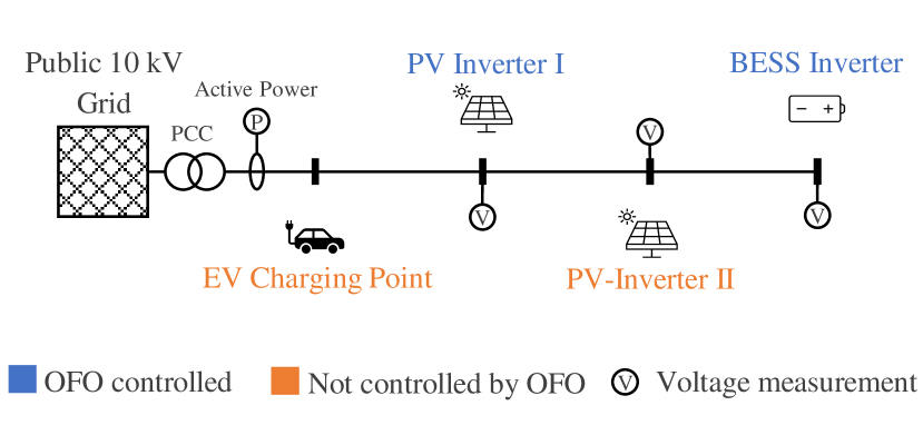
Figure 2: Laboratory setup used for the experimental validation. PV inverter I is connected to bus 3, PV inverter II is connected to bus 1, and the BESS inverter is connected to bus 2. The figure is taken from [7].

III Introduction to Online Feedback Optimization

In this section, we give a quick introduction to OFO. Consider a system with inputs $u$, disturbances $d$, and outputs $y=h(u,d)$, where $h(\cdot,\cdot)$ describes the behavior of the system. In our use case, the input is $u=\begin{bmatrix}p\\ q\end{bmatrix}$, where $p$ and $q$ are the active and reactive power commands to the FPU. The output is $y=\begin{bmatrix}v\\ p_{PCC}\end{bmatrix}$, where $v$ are the measured voltage magnitudes in the grid and $p_{PCC}$ is the active power flow over the PCC. The goal of OFO is to bring the inputs $u$ of the system to an optimal operating point $u^{\star}$. This optimal point is defined through an optimization problem for example:

$$\min_{u,y} \Phi(u,y)$$ (1)

s. t. $$u_{min}\leq u\leq u_{max}$$

$$y_{min}\leq y\leq y_{max}$$

$$y=h(u,d)$$

OFO is a feedback control method that uses optimization algorithms to solve such optimization problems. It is important to note that, OFO does not calculate $u^{\star}$ offline and based on a model but iteratively and online. This means the inputs $u(k)$, which are applied to the real system, are changed over time until they have converged to the solution of the optimization problem $u^{\star}$. This makes the approach robust to model mismatch, computationally light, and nearly model free [8].
The type of OFO controller we use in this paper is based on projected gradient descent. It consists of the integral controller ${u(k+1)=u(k)+\sigma(u,d,y_{m})}$ and an underlying quadratic problem (QP)

$$\sigma(u,d,y_{m})\coloneqq\arg \min_{w\in\mathbb{R}^{p}}\,\|w+G^{-1}H(u,d)^{T}\nabla\Phi(u,y_{m})\|^{2}_{G}$$ (2)

s.t. $$u_{min}\leq u(k)+w<u_{max}$$

$$y_{min}\leq y_{m}(k)+\nabla_{u}h(u,d)w<y_{max}$$

with $w=\begin{bmatrix}\Delta p\\ \Delta q\end{bmatrix}$, the tuning matrix $G$, and $H(u,d)^{T}=[I_{n}\,\nabla_{u}h(u,d)^{T}]$ where $n$ is the number of entries in $u$ and $()^{T}$ denotes the transpose. The term $\nabla_{u}h(u,d)$ is the gradient of $y$ with respect to $u$. It is a linear approximation of $h(\cdot,\cdot)$ and describes how a change in $u$ affects $y$. In this paper, it describes how changes in $p$ and $q$ change the voltages $v$ and the power flow $p_{PCC}$. Therefore $\nabla_{u}h(u,d)$ consists of power transfer distribution factors and other sensitivities. We define $H_{p}=\begin{bmatrix}\nabla_{p}p_{PCC}(p,q,d)\\ \nabla_{q}p_{PCC}(p,q,d)\end{bmatrix}\approx\begin{bmatrix}\nabla_{p}p_{PCC}(p,q,d)\\ 0\end{bmatrix}$ and $H_{v}=\begin{bmatrix}\nabla_{p}v(p,q,d)\\ \nabla_{q}v(p,q,d)\end{bmatrix}$. Note that, both $H_{p}$ and $H_{v}$ can be approximated by a constant vector or matrix, respectively. We calculate such approximations offline for a fixed initial operating point using a model of the grid and use these same sensitivity values throughout the paper and all experiments. This is possible because OFO is robust against model mismatch in these sensitivities [9].
Overall, the setup is as depicted in the block diagram that can be seen in Figure 3.

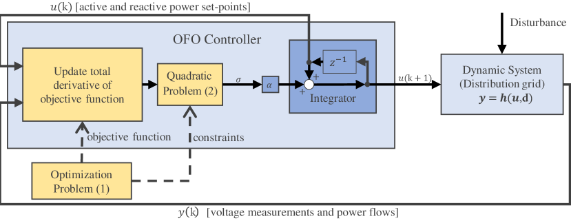
Figure 3: Block diagram of an OFO controller. The OFO controller iteratively changes $u$ until the solution of the optimization problem is reached. The figure is adapted from [7].

The OFO controller is implemented in a centralized location. It receives voltage measurements $v$ and a measurement of the active power flow over the PCC $p_{PCC}$. Based on these measurements the OFO controller updates the active power $p$ and reactive power $q$ setpoints for the inverters. To calculate the update, the OFO controller solves a quadratic problem that is easy to solve even for large numbers of variables which means the setup scales very well with the system size. The updated $p$ and $q$ setpoints are then communicated to the inverters. Within a few iterations, $p$ and $q$ converge to the optimal solution of the overarching optimization problem.

IV Optimization Problems for Distribution Grid Flexibility

The FPU are supposed to deliver the requested flexibility $P_{set}$ at the PCC while all voltages $v$, active power injections $p$, and reactive power injections $q$ are within their limits. Generally, we can either encode this into the cost function or the constraints of the optimization problem (1). We refer to these two options as cost approach and constraint approach. Based on our experimental results, we can later on give a clear recommendation on which approach is favorable.

IV-A Cost Approach

In the cost approach, we encode the goal of providing flexibility in the cost function as follows

$$\min_{p,q} (p_{set}-p_{PCC}(p,q))^{2}$$ (3)

s. t. $$p_{min}\leq p\leq p_{max}$$

$$q_{min}\leq q\leq q_{max}$$

$$v_{min}\leq v(p,q,d)\leq v_{max}$$

The OFO controller then is $u(k+1)=\begin{bmatrix}p(k+1)\\ q(k+1)\end{bmatrix}=\begin{bmatrix}p(k)\\ q(k)\end{bmatrix}+\sigma(u,d,y_{m})$ with

$$\sigma(u,d,y_{m})\coloneqq\arg\min_{w\in\mathbb{R}^{n}} \|w+2G^{-1}H_{p}(p_{set}-p_{PCC}(p,q)))\|^{2}_{G}$$ (4)

s. t. $$\begin{bmatrix}p_{min}\\ q_{min}\end{bmatrix}\leq\begin{bmatrix}p(k)\\ q(k)\end{bmatrix}+w\leq\begin{bmatrix}p_{max}\\ q_{max}\end{bmatrix}$$

$$v_{min}\leq v_{meas}(k)+H_{v}w\leq v_{max}$$

IV-B Constraint Approach

In the constraint approach, we encode the goal of providing flexibility through the constraints $P_{set}=p_{PCC}$. Therefore, we can use the cost function to further specify what we consider the optimal behavior of our power grid. Here we consider a minimal use of active and reactive power to be optimal and therefore define

$$\min_{p,q} p^{T}p+q^{T}q$$ (5)

s. t. $$p_{min}\leq p\leq p_{max}$$

$$q_{min}\leq q\leq q_{max}$$

$$v_{min}\leq v(p,q)\leq v_{max}$$

$$p_{set}=p_{PCC}(p,q)$$

The OFO controller then is $u(k+1)=\begin{bmatrix}p(k+1)\\ q(k+1)\end{bmatrix}=\begin{bmatrix}p(k)\\ q(k)\end{bmatrix}+\sigma(u,d,y_{m})$ with

$$\sigma(u,d,y_{m})\coloneqq\arg \min_{w\in\mathbb{R}^{n}}\,\|w+2G^{-1}\begin{bmatrix}p(k)\\ q(k)\end{bmatrix}\|^{2}_{G}$$ (6)

s. t. $$\begin{bmatrix}p_{min}\\ q_{min}\end{bmatrix}\leq\begin{bmatrix}p(k)\\ q(k)\end{bmatrix}+w\leq\begin{bmatrix}p_{max}\\ q_{max}\end{bmatrix}$$

$$v_{min}\leq v_{meas}+H_{v}w\leq v_{max}$$

$$p_{set}=p_{PCC}(k)+H_{p}w$$

V Controller Tuning

We will now have a closer look at how OFO controllers work. This will become important when we aim to tune them through the matrix $G$. Note that, $G$ only affects the solution of the underlying QP inside the OFO controller but does not affect the solution of the overarching optimization problem[28]. In other words: The overarching optimization problem defines how the system is supposed to operate and $G$ can be used to adjust how the OFO controller converges to this operating point. In the following we focus on tuning $G$.
Consider the QP in (2). The cost function is a norm and therefore positive or zero. Without active constraints, the solution of the QP can be chosen as

$$\begin{split}w&=-G^{-1}H(u)^{T}\nabla\Phi(u,y)\\ &=-G^{-1}\nabla_{u}\Phi(h(u,d))\end{split}$$ (7)

and the cost function is then zero and therefore minimized. This means, that if the constraints are not active, the controller integrates the gradient of the cost function of the overarching optimization problem multiplied with $G^{-1}$. Hence, this is a gradient descent scheme that keeps changing $u$ until the gradient is zero and has therefore converged to an unconstrained (local) minimum of (3). The matrix $G^{-1}$ can be used to tune the convergence behavior. The smaller the entries in $G$, the faster the convergence.
The behavior is different when there are active constraints, e.g. a voltage reaches its limit. Then certain entries of $w$ need to deviate from the unconstrained solution to guarantee that the active constraint is not violated. Then the optimal solution of the QP in (2) is a vector $w$ that satisfies the constraints and is ”as close as possible” to $-G^{-1}H(u)^{T}\nabla\Phi(u,y)$. Using the tuning matrix $G$ we can decide what close in this context means. This becomes more apparent when we multiply out the cost function of the QP:

$$\begin{split}\|w+&G^{-1}\nabla_{u}\Phi(u)\|^{2}_{G}\\ &=w^{T}Gw+2w^{T}\nabla_{u}\Phi(u)+\nabla_{u}\Phi(u)^{T}G^{-1}\nabla_{u}\Phi(u)\end{split}$$

We can see that the tuning matrix $G$ is a tuning weight in the term $w^{T}Gw$. Therefore, small values of $G$ lead to a small weight on the corresponding entry in $w$, and the QP can make these entries in $w$ large while still keeping the cost function of the QP small. Therefore, if an element of $w$ has to deviate from the unconstrained optimal solution it will be these entries of $w$. Overall, $G$ gives us a way to tune which descent direction of the overarching optimization problem we care about most.

We will furthermore explain the tuning of $G$ by having a look at the cost approach and the resulting OFO controller in (4). Figure 4 shows the convergence behavior of the OFO controller with $G=I$ for the cost approach.

Figure 4: Extremely slow convergence of the cost approach with $G=I$.

Figure 5: Fast convergence of the cost approach due to a tuned $G$ matrix.

In the beginning, the controller quickly changes the active power setpoints to track $P_{set}=-14.5$ kW while the reactive power setpoints stay small. Then the convergence becomes very slow once the voltage at the BESS inverter (bus 2) reaches its upper level (dashed turquoise line). From this point onward a voltage constraint in the QP in (4) is active. Changing the active power injections to further minimize the cost function of the overarching optimization problem (3) is now only possible if reactive power is used to counteract the voltage rise due to the active power increase. Because a change in the reactive powers $q$ will not affect the cost function ($\nabla_{q}p_{PCC}\approx 0$), the unconstrained solution for $w$ is to not change the reactive power injections. Therefore, the QP does not want to change $q$. However, without changing $q$ we cannot change $p$ because that would lead to voltage violations. By putting small values in the entries of $G$ corresponding to $q$ the QP can change $q$ without a large effect on the cost function of the QP. Then the optimal solution of the QP will be to make larger changes to the reactive power injections which allow for larger changes in the active power injections $p$. Figure 5 shows the behavior of the cost approach with

$$G=\begin{bmatrix}I_{2}&0\\ 0&10^{-10}\cdot I_{2}\end{bmatrix},$$

where $I_{2}$ is an identity matrix of size $2\times 2$. The figure shows that the convergence is significantly improved because the reactive power injections $q$ are changed faster which allows for faster changes in $p$ and therefore convergence of $p_{PCC}$ to the flexibility setpoint $p_{set}$. Within three iterations of the OFO controller, the distribution grid successfully delivers the requested flexibility to the upper-level grid. Furthermore, the constraints within the distribution grid are satisfied. We conclude that $G$ must be used to tune the convergence behavior of an OFO controller. When constraints become active then tuning $G$ is even more important, because otherwise the convergence speed can be significantly affected.

VI Results

In this section, we present the results of the constraint approach and compare it to the behavior of the cost approach. Furthermore, we show the interaction of an OFO controller with an inverter in the grid that is not part of the OFO control but performs voltage control according to VDE4105 [29]. Finally, we also add a charging electric vehicle which enables us to test our OFO controller on a real grid with real loads.

Figure 6: Control performance of the constraint approach.

VI-A Performance of the Constraint Approach

In Figure 6 it can be seen that the convergence of the constraint approach is nearly immediate. After 10 seconds, which is two iterations of the controller, the setpoint is tracked. Again, all constraints are satisfied and therefore the grid is providing the requested flexibility while operating the distribution grid within its operational limits. The convergence is even faster than with the cost approach but the main difference is the use of reactive power. In the cost approach, there is no penalty on the use of reactive power leading to a high reactive power usage. In the constraint approach, the usage of reactive power is part of the cost function of the overarching control problem (5) and therefore the OFO controller is encouraged to limit the use of reactive power. This leads to the following behavior that can be seen in Figure 6: The active power setpoints for the two inverters are not the same. The inverter at the end of the line is utilized less because its active power injection leads to a voltage increase at its point of connection (bus 2) that would need to be compensated by using reactive power. Given that these reactive power flows lead to active power losses it is advantageous to limit the use of reactive power and therefore losses. With the constraint approach, the losses are significantly lower than with the cost approach. This becomes apparent when we compare the active power injections of the inverters. To deliver -14.5 kW of flexibility to the upper-level grid the inverters change their active power injections by $-4-11=-15$ kW in the constraint approach and by $-9.2-9.2=-18.4$ kW in the cost approach. This highly non-trivial solution of utilizing inverters differently depending on where they are located in the grid is a remarkable behavior of the controller which is able to derive this solution solely based on the approximate sensitivities $H_{p}$ and $H_{v}$ and feedback from the grid through measurements. Also note that, if the distribution grid is not able to provide the requested flexibility the QP in the constraint approach becomes infeasible. This is because $p_{set}=p_{PCC}$ is a hard constraint of the QP. This infeasibility can be used as a signal to communicated to the entity requesting the flexibility that this is currently not possible. The QP in the cost approach does not become infeasible because the goal of $p_{set}=p_{PCC}$ is included in the cost function and does therefore not have this feature.
Overall, the constraint approach is faster and uses the inverters more efficiently.

VI-B Interaction with other Inverters in the Grid

We will now show and analyze how the OFO controller with the constraint approach interacts with other devices in the grid. For that, we add the PV-Inverter II to the setup. This inverter is injecting a changing amount of active power into the grid and operates a $q(v)$ voltage control according to VDE4105 [29] with a deadband of 3%.
The task is to provide a flexibility of -15 kW at the PCC. The dashed orange line in Figure 7 shows that deviations from the setpoint are immediately mitigated in the next time step, meaning once the controller detects a deviation it fixes it within one sampling interval and accurately. Figure 7 shows that small voltage violations can occur when the independent PV inverter II changes its active power injections. Also, these violations are mitigated within one time step of the controller which is well within the timespan of the current norms [29]. Overall, the OFO controller interacts well with the other inverter in the grid.

Figure 7: Interaction of the OFO controller with an inverter injecting a varying amount of power and which is controlling its reactive power according to VDE4105 [29].

VI-C Fully Realistic Test Setup

To go one step further, we add the EV charging point to the grid and connect an electric vehicle. The requested flexibility setpoint at the PCC is now -2 kW. The collected data can be seen in Figure 8. The setpoint is tracked well. The only noticeable deviations are in the beginning and end when the EV continuously changes its active power intake. This is because the OFO controller is not aware of the changing power consumption of the EV. Actually, the OFO controller does not even know that there is an EV charging point in the grid. Therefore, the OFO controller can only react to the effect of the changing power consumption which leads to a small tracking error. However, this is not specific to the OFO control method but the ramp-like disturbance that the charging EV represents. The voltages are kept within their limits and violations are mitigated quickly.

Figure 8: An electric vehicle is charged and the OFO controller counteracts this disturbance such that the distribution grid accurately provides the requested flexibility while satisfying the distribution grid constraints.

VII Conclusion

In this paper, we used an OFO controller to disaggregate a flexibility request onto FPUs. Using a real distribution grid setup we showed that tuning the matrix $G$ of the OFO controller is essential for fast convergence and good performance and we explained how to tune $G$ in detail. We compared two possible approaches to phrase the disaggregation task as an optimization problem and can conclude that the constraint approach outperforms the cost approach. The better performance is in terms of losses in the grid and the constrained approach is more versatile as its cost function can be used to parameterize the favored behavior of the system. Also the constraint approach will realize if the distribution grid cannot provide the requested flexibility and can signal this to the entity requesting the flexibility. Furthermore, the experiments showed that the tuned OFO controller is compatible with other control devices in the grid and enables fast delivery of the requested flexibility while guaranteeing the operational limits in the distribution grid. Also, the method is robust to model mismatch and changing consumption in the distribution grid while it is able to utilize the full flexibility of the distribution grid. Overall, OFO with the constraint approach is a powerful tool to disaggregate flexibility requests onto FPUs in a distribution grid.

References

- [1] “Innosys 2030 – innovations in system operation up to 2030 - short report on the joint project,” Tech. Rep., 2022. [Online]. Available: https://www.innosys2030.de/wp-content/uploads/InnoSys-ShortReport-EN.pdf
- [2] T. Kolster, R. Krebs, S. Niessen, and M. Duckheim, “The contribution of distributed flexibility potentials to corrective transmission system operation for strongly renewable energy systems,” Applied Energy, vol. 279, p. 115870, 2020.
- [3] J. Silva, J. Sumaili, R. J. Bessa, L. Seca, M. A. Matos, V. Miranda, M. Caujolle, B. Goncer, and M. Sebastian-Viana, “Estimating the active and reactive power flexibility area at the tso-dso interface,” IEEE Transactions on Power Systems, vol. 33, no. 5, pp. 4741–4750, 2018.
- [4] H. Früh, S. Müller, D. Contreras, K. Rudion, A. von Haken, and B. Surmann, “Coordinated vertical provision of flexibility from distribution systems,” IEEE Transactions on Power Systems, vol. 38, no. 2, pp. 1832–1842, 2022.
- [5] T. Kolster, S. Niessen, and M. Duckheim, “Providing distributed flexibility for curative transmission system operation using a scalable robust optimization approach,” Electric Power Systems Research, vol. 211, p. 108431, 2022.
- [6] X. Chen and N. Li, “Leveraging two-stage adaptive robust optimization for power flexibility aggregation,” IEEE Transactions on Smart Grid, vol. 12, no. 5, pp. 3954–3965, 2021.
- [7] F. Klein-Helmkamp, F. Böhm, L. Ortmann, A. Winkens, F. Schmidtke, S. Bolognani, F. Dörfler, and A. Ulbig, “Providing curative distribution grid flexibility using online feedback optimization,” in 2023 IEEE PES Innovative Smart Grid Technologies Europe (ISGT EUROPE), 2023, pp. 1–5.
- [8] A. Hauswirth, S. Bolognani, G. Hug, and F. Dörfler, “Optimization algorithms as robust feedback controllers,” arXiv:2103.11329, 2021.
- [9] L. Ortmann, A. Hauswirth, I. Caduff, F. Dörfler, and S. Bolognani, “Experimental validation of feedback optimization in power distribution grids,” Electric Power Systems Research, vol. 189, p. 106782, 2020.
- [10] J. C. Olives-Camps, Á. R. del Nozal, J. M. Mauricio, and J. M. Maza-Ortega, “A model-less control algorithm of dc microgrids based on feedback optimization,” International Journal of Electrical Power & Energy Systems, vol. 141, p. 108087, 2022.
- [11] S. Nowak, Y. C. Chen, and L. Wang, “A measurement-based gradient-descent method to optimally dispatch der reactive power,” in 2020 47th IEEE Photovoltaic Specialists Conference (PVSC). IEEE, 2020, pp. 0028–0032.
- [12] L. Gan and S. H. Low, “An online gradient algorithm for optimal power flow on radial networks,” IEEE Journal on Selected Areas in Communications, vol. 34, no. 3, pp. 625–638, 2016.
- [13] E. Dall’Anese and A. Simonetto, “Optimal power flow pursuit,” IEEE Transactions on Smart Grid, vol. 9, no. 2, pp. 942–952, 2016.
- [14] J. C. Olives-Camps, Á. R. del Nozal, J. M. Mauricio, and J. M. Maza-Ortega, “A holistic model-less approach for the optimal real-time control of power electronics-dominated ac microgrids,” Applied Energy, vol. 335, p. 120761, 2023.
- [15] Z. Tang, E. Ekomwenrenren, J. W. Simpson-Porco, E. Farantatos, M. Patel, and H. Hooshyar, “Measurement-based fast coordinated voltage control for transmission grids,” IEEE Transactions on Power Systems, vol. 36, no. 4, pp. 3416–3429, 2020.
- [16] A. Bernstein and E. Dall’Anese, “Real-time feedback-based optimization of distribution grids: A unified approach,” IEEE Transactions on Control of Network Systems, vol. 6, no. 3, pp. 1197–1209, 2019.
- [17] S. Zhan, J. Morren, W. v. d. Akker, A. v. d. Molen, N. G. Paterakis, and J. G. Slootweg, “Fairness-incorporated online feedback optimization for real-time distribution grid management,” IEEE Transactions on Smart Grid, pp. 1–1, 2023.
- [18] J. Wang, M. Blonsky, F. Ding, S. C. Drew, H. Padullaparti, S. Ghosh, I. Mendoza, S. Tiwari, J. E. Martinez, J. J. Dahdah et al., “Performance evaluation of distributed energy resource management via advanced hardware-in-the-loop simulation,” in Innovative Smart Grid Technologies Conference (ISGT). IEEE, 2020, pp. 1–5.
- [19] H. Padullaparti, A. Pratt, I. Mendoza, S. Tiwari, M. Baggu, C. Bilby, and Y. Ngo, “Peak load management in distribution systems using legacy utility equipment and distributed energy resources,” in 2021 IEEE Green Technologies Conference (GreenTech). IEEE, 2021, pp. 435–441.
- [20] L. Ortmann, A. Prostejovsky, K. Heussen, and S. Bolognani, “Fully distributed peer-to-peer optimal voltage control with minimal model requirements,” Electric Power Systems Research, vol. 189, p. 106717, 2020.
- [21] L. Reyes-Chamorro, A. Bernstein, N. J. Bouman, E. Scolari, A. M. Kettner, B. Cathiard, J.-Y. Le Boudec, and M. Paolone, “Experimental validation of an explicit power-flow primary control in microgrids,” IEEE Transactions on Industrial Informatics, vol. 14, no. 11, pp. 4779–4791, 2018.
- [22] B. Kroposki, A. Bernstein, J. King, D. Vaidhynathan, X. Zhou, C.-Y. Chang, and E. Dall’Anese, “Autonomous energy grids: Controlling the future grid with large amounts of distributed energy resources,” IEEE Power and Energy Magazine, vol. 18, no. 6, pp. 37–46, 2020.
- [23] B. Kroposki, A. Bernstein, J. King, and F. Ding, “Good grids make good neighbors,” IEEE Spectrum, vol. 57, no. NREL/JA-5D00-78521, 2020.
- [24] L. Ortmann, C. Rubin, A. Scozzafava, J. Lehmann, S. Bolognani, and F. Dörfler, “Deployment of an online feedback optimization controller for reactive power flow optimization in a distribution grid,” in 2023 IEEE PES Innovative Smart Grid Technologies Europe (ISGT EUROPE), 2023, pp. 1–6.
- [25] BDEW, “Redispatch in deutschland,” Tech. Rep., 2023. [Online]. Available: https://www.bdew.de/media/documents/BDEW-Redispatch_Bericht_2023_zum_Berichtsjahr_2022.pdf
- [26] I. Hacker, F. Schmidtke, D. van der Velde, and S. T. Czyrnik, “A framework to evaluate multi-use flexibility concepts simultaneously in a co-simulation environment and a cyber-physical laboratory.” 2021.
- [27] F. Schmidtke, I. Hacker, C. Vertgewall, and A. Ulbig, “Evaluation of multi-use charging strategies in a time-dependent co-simulation environment for behind-the-meter flexibility,” in CIRED Porto Workshop 2022: E-mobility and power distribution systems, vol. 2022. IET, 2022, pp. 779–783.
- [28] V. Häberle, A. Hauswirth, L. Ortmann, S. Bolognani, and F. Dörfler, “Non-convex feedback optimization with input and output constraints,” IEEE Control Systems Letters, vol. 5, no. 1, pp. 343–348, 2020.
- [29] “VDE-AR-N 4105: Generators connected to the LV distribution network – Technical requirements for the connection to and parallel operation with low-voltage distribution networks,” 2018.