Contextuality, superlocality and supernoncontextuality

Abstract

Contextuality is a fundamental manifestation of nonclassicality, indicating that for certain quantum correlations, sets of jointly measurable variables cannot be pre-assigned values independently of the measurement context. In this work, we characterize nonclassical quantum correlation beyond contextuality, in terms of supernoncontextuality, namely the higher-than-quantum hidden-variable(HV) dimensionality required to reproduce the given noncontextual quantum correlations. Thus supernoncontextuality is the contextuality analogue of superlocality. Specifically, we study the quantum system of two-qubit states in a scenario composed of five contexts that demonstrate contextuality in a state-dependent fashion. For this purpose, we use the framework of boxes, whose behavior is described by a set of probabilities satisfying the no-disturbance conditions. We observe that superlocal states must have sufficiently a high HV dimension in order to lead to a contextual box. On the other hand, a noncontextual superlocal box can be supernoncontextual, but superlocality is not a necessary condition. For sublocal (i.e., not superlocal) boxes, supernoncontextuality arises owing to a different type of simultaneous correlation in two MUBs present in any nonproduct state and correlations due to nonlocal measurements. From an operational perspective, the superlocal states that can or cannot be used to demonstrate contextuality can be distinguished by quantum correlations in two and three mutually unbiased bases (MUBs) of the discordant correlations in the states.

1 Introduction

The observation of quantum systems admits certain correlations with features that defy classical intuition. Such correlations can come in two setups: Bell scenarios [1] and Kochen-Specker scenarios [2]. In a Bell scenario, outcomes are observed locally on a composite system, whilst on the other hand, in a Kochen-Specker scenario, outcomes are observed in a non-contextual way on a single system that does not have subsystems or a composite system that need not admit a spatial separation between the subsystems. In such scenarios, an outstanding question introduced at the time [3] was whether predefined values to the outcomes could be assigned based on a hidden variable description. Remarkably, it was shown by Bell that the correlations between the outcomes of quantum measurements in an appropriate setup can violate an inequality based on locality and realism [4]. This phenomenon is referred to as Bell non-locality of quantum correlations [1]. On the other hand, Kochen and Specker proposed a setup of a certain set of quantum measurements on a quantum system, on which, they showed a logical contradiction with predefined value assignments originating from a hidden variable in a non-contextual way [5]. Such yet another remarkable discovery is called Kochen-Specker contextuality of quantum correlations [2]. Just like Bell inequalities, detecting Kochen-Specker contextuality based on an inequality satisfied by any non-contextual hidden variable model was also proposed [6, 7, 8].

The quantum advantage of quantum correlations due to Bell nonlocality is shown against local-hidden-variable (LHV) models [9], or, in other words, Bell non-locality of quantum correlations provides certification of relevant properties in a Bell scenario in a device-independent way, i.e., without describing the Hilbert-space dimension of the quantum system and the quantum measurements used to demonstrate the phenomenon [10, 11]. This remarkable certification offered by Bell non-locality powers genuinely quantum information protocols such as device-independent quantum key distribution [12] device-independent certification of randomness [11, 13], random access coding using Bell-nonlocal correlations [14, 15, 16] and device-independent certification of quantum devices (such as entangled states, incompatible measurements and quantum channels) [17, 18, 19]. Quantum information protocols such as quantum computation, quantum cryptography and quantum communication for which quantum advantage is powered by Kochen-Specker contextuality have also been explored [20, 21, 22, 23, 24], see also Sec. VI in Ref. [2]. Based on contextuality, certification of quantum devices for quantum computation has been shown in a dimension-independent way [25, 26, 27, 28, 29, 30, 31]. A quantum computation device that has such certification in it provides the computational power to have genuine quantum advantage [32]; otherwise, it is hard to believe that it is truly a quantum computer [33].

Quantum correlations in a Bell scenario have also been studied in a dimension-bounded way. In this context, super-locality refers to a quantum advantage in simulating certain boxes that have a local-hidden-variable model in terms of the dimension of the quantum system against that of the hidden variable [34, 35, 36]. In Refs. [37, 38], the authors studied in a specific scenario superunsteerability, which is an extension of super-locality to steering scenarios [39, 40]. Such studies provide a better understanding of quantum steering and quantum correlations due to quantum discord [41, 42]. Superlocality or superunsteerability also acts as a resource for quantum advantage in certain quantum information protocols in the presence of a finite amount of shared classical randomness [43, 44, 45]. It would be interesting to extend the concept of superlocality to contextuality scenarios to identify useful new applications and a useful new understanding of quantum contextuality.

In this work, we characterize these correlations beyond the contextuality of two-qubit states in a scenario that demonstrates contextuality in a state-dependent fashion which is considered by Peres [46]. To this end, we adapt the box framework of contextuality to this scenario. We identify that quantum correlations based on superlocality can act as a resource for contextuality. While we observe that certain superlocal states with the minimal hidden variable dimension $4$, in the context of a Bell scenario with two-input and two-output on each side, can lead to contextuality, there are superlocal states with the minimal hidden variable dimension $3$ that do not imply contextuality. We also note that these two types of superlocal states can be distinguished by the simultaneous correlations in two and three MUBs, as studied in Ref. [47], respectively. We next introduce the concept of supernoncontextuality as the extension of superlocality to contextuality scenarios. Supernoncontextuality indicates a quantum advantage in using a quantum system of lower Hilbert space dimension to simulate the box over the requirement of higher dimensionality of the noncontextual hidden variable model required to simulate it. We provide two examples of supernoncontextual boxes that imply quantum correlation beyond contextuality in the above-mentioned contextuality scenario. For one of these examples, superlocality of the two-qubit state that does not imply contextuality acts as a resource. In our other example of supernoncontextuality, we demonstrate that superlocality is not necessary for supernoncontextuality, but quantum correlation beyond discord as captured by simultaneous correlations in two MUBs [48], and correlation due to nonlocal measurements, act as a resource.

2 Preliminaries

2.1 Quantum correlation beyond entanglement and discord

Quantum discord captures quantum correlations beyond entanglement [41, 42]. Let $D^{\rightarrow}(\rho_{AB})$ denote quantum discord as from Alice to Bob, on the other hand, quantum discord from Bob to Alice is denoted as $D^{\leftarrow}(\rho_{AB})$. Quantum discord from Alice to Bob, $D^{\rightarrow}(\rho_{AB})$, vanishes for a given $\rho_{AB}$ if and only if (iff) it is a classical-quantum (CQ) state of the form,

$$\rho_{\texttt{CQ}}=\sum_{i}p_{i}\ket{i}\bra{i}_{A}\otimes\rho^{(i)}_{B},$$ (1)

where $\{\ket{i}\}$ forms an orthonormal basis on Alice’s Hilbert space and $\rho^{(i)}_{B}$ are any quantum states on Bob’s Hilbert space. On the other hand, $D^{\leftarrow}(\rho_{AB})$ vanishes for a given $\rho_{AB}$ iff it is a quantum-classical (QC) state of the form,

$$\rho_{\texttt{QC}}=\sum_{i}p_{i}\rho^{(i)}_{A}\otimes\ket{i}\bra{i}_{B},$$ (2)

where now $\{\ket{i}\}$ forms an orthonormal basis on Bob’s Hilbert space and $\rho^{(i)}_{A}$ are any quantum states on Alice’s Hilbert space. A CQ state can have one-way discord as measured through $D^{\leftarrow}(\rho_{AB})$, on the other hand, a QC state can have one-way discord as measured through $D^{\rightarrow}(\rho_{AB})$. A quantum-quantum (QQ) state which has a nonzero discord both ways is neither a CQ state nor a QC state. A classically-correlated (CC) state which has two-way zero discord has the form,

$$\rho_{\texttt{CC}}=\sum_{i}p_{i}\ket{i}\bra{i}_{A}\otimes\ket{i}\bra{i}_{B}.$$ (3)

In the above three equations, $p_{i}\geq 0$ with $\sum_{i}p_{i}=1$.

Classical correlation of a bipartite state $C(\rho_{AB})$ as used in the definition of quantum discord [42] is calculated as the maximal correlation obtained from a certain optimal basis measured on one side of the bipartite system. The amount of correlation is captured by the Holevo quantity of the ensemble prepared on the other side of the bipartite system. Let $\{\ket{a_{i}},i=0,1,\cdots,d-1\}$ be a basis measured on Alice’s side of the bipartite state $\rho_{AB}$. The ensemble prepared on Bob’s side due to this measurement is given by $\{p(a_{i});\rho^{(i)}_{B}\}$, where $p(a_{i})=\mathrm{Tr}\left(\ket{a_{i}}\bra{a_{i}}\otimes\mathbbm{1}\rho_{AB}\right)$ is the probability of obtaining an outcome $a_{i}$ and $\rho^{B}_{i}=\mathrm{Tr}_{A}\left(\ket{a_{i}}\bra{a_{i}}\otimes\mathbbm{1}\rho_{AB}\right)$ is a conditional state prepared on Bob’s side corresponding to the outcome $a_{i}$. Then, the Holevo quantity of this ensemble prepared on Bob’s side is given by $\chi(p(a_{i});\rho^{(i)}_{B})=S(\sum_{i}p(a_{i})\rho^{i}_{B})-p(a_{i})S(\sum_{i}\rho^{i}_{B})$, where $S(\cdot)$ is the von Neumann entropy of the density matrix. Classical correlation denoted as $C_{1}(\rho_{AB})$ is given by

$$C_{1}(\rho_{AB})=\max_{\{\ket{a_{i}}\}}\chi\left(p(a_{i});\rho^{i}_{B}\right),$$ (4)

where the maximization is performed over all bases. Considering another set of bases which are mutually unbiased to the basis that provides classical correlation $C_{1}(\rho_{AB})$, the maximal correlation obtained from a certain optimal choice of the second basis, denoted $Q_{2}$, as quantified in the case of classical correlation mentioned above, was studied in Ref. [47]. This quantity is used to capture quantum correlation in simultaneous correlations in two MUBs. Considering the third set of bases that is mutually unbiased to the bases that provide $C_{1}$ and $Q_{2}$, another measure of quantum correlation, denoted $Q_{3}$, is also introduced to characterize simultaneous correlations in three MUBs. If there are $n$ MUBs for the quantum system, the series of measures $Q_{1}$, $Q_{2}$, $\cdots$ $Q_{n}$ can be used to capture different quantum correlations due to a nonzero discord [47].

Quantum correlations in terms of the simultaneous correlations in MUBs of the discordant correlations in two-qubit states can be characterized using $Q_{2}$ and $Q_{3}$. In Ref. [47], nonzero values of $Q_{2}$ and $Q_{3}$ for the Bell-diagonal two-qubit states were presented. In this work, we consider the two-qubit Werner state given by

$$\rho_{W}=W|\psi^{\texttt{me}}_{2}\rangle\langle\psi^{\texttt{me}}_{2}|+(1-W)\frac{\bf{1}_{4}}{4},$$ (5)

where $\ket{\psi^{\texttt{me}}_{2}}$ is the maximally entangled state of a two-qubit system given by the Bell state

$$\ket{\psi^{\texttt{me}}_{2}}=\frac{1}{\sqrt{2}}(\ket{00}+\ket{11})$$ (6)

and $\bf{1}_{4}$ is the identity operator of two-qubit Hilbert space. The one-parameter family of states is entangled iff $W>1/3$ [49] and has a nonzero quantum discord for any $W>0$ [41, 42]. The Werner states belong to the broader family of states, the Bell-diagonal states mentioned above.

Simultaneous correlations in MUBs are also present in any nonproduct state. Extending the measures of quantum correlations studied in Ref. [47] which are zero for one-way zero discord states, in Ref. [48], the measures of quantum correlations to capture the amount of simultaneous correlations in MUBs in any nonproduct state, denoted $C_{2}$, $C_{3}$, $\cdots$, $C_{n}$, were studied. Here $C_{2}$ denotes the maximal correlation as quantified in the definition of $Q_{2}$, but optimized over a set of bases which are mutually unbiased to any basis which is not the basis that quantifies $C_{1}$. Variable $C_{3}$ is defined as the maximal correlation due to a third basis that is mutually unbiased to the bases that quantify $C_{1},C_{2}$ and similarly, other quantities $C_{4}$, $\cdots$, $C_{n}$ are defined recursively, provided that the $n$ MUBs, with $n\geq 4$, exist for the system (It is known that for a system of prime power dimension $q$, there are $q+1$ MUBs).

Let $\bf{1}_{2}$, $X_{2}$, $Y_{2}$ and $Z_{2}$ denote the identity operator acting on qubit Hilbert space and the Pauli operators given by $X_{2}=\ket{0}\bra{1}+\ket{1}\bra{0}$, $Y_{2}=-i\ket{0}\bra{1}+i\ket{1}\bra{0}$ and $Z_{2}=|0\rangle\langle 0|-|1\rangle\langle 1|$, respectively. Consider a CC state given by

$$\rho_{\texttt{CC}}=\frac{1}{2}(|00\rangle\langle 00|+|11\rangle\langle 11|).$$ (7)

Classical correlation $C_{1}$ of the above state is achieved by the basis of $Z_{2}$. For this state, $Q_{2}=Q_{3}=0$. Whereas, for this state, quantum correlation in general MUBs, $C_{2}$ and $C_{3}$, takes a nonzero value and arises due to the presence of the simultaneous correlations in two MUBs which are that of the observables in $\{\frac{Z_{2}+X_{2}}{\sqrt{2}},\frac{Z_{2}-X_{2}}{\sqrt{2}}\}$ and three MUBs which are that of the observables in $\{\frac{Z_{2}+X_{2}+Y_{2}}{\sqrt{3}},\frac{Z_{2}+X_{2}-Y_{2}}{\sqrt{3}},\frac{Z_{2}-X_{2}+Y_{2}}{\sqrt{3}}\}$, respectively [48].

2.2 Quantum correlation beyond Bell nonlocality

In a Bell scenario where two spatially separated observers Alice has access to inputs $x$ and observes outputs $a$ and Bob has access to inputs $y$ and observes outputs $b$, a bipartite box $P$ = $P(ab|xy)$ := $\{p(ab|xy)\}_{a,x,b,y}$ is the set of joint probability distributions $p(ab|xy)$ for all possible $a$, $x$, $b$, $y$. Such a bipartite box that can be observed in a Bell scenario satisfies the no-signaling (NS) conditions. The single-partite box $P(a|x)$ := $\{p(a|x)\}_{a,x}$ of a NS box $P(ab|xy)$ is the set of marginal probability distributions $p(a|x)$ for all possible $a$ and $x$; which are given by,

$$p(a|x)=\sum_{b}p(ab|xy),\quad\forall a,x,y.$$ (8)

The single-partite box $P(b|y)$ := $\{p(b|y)\}_{b,y}$ of a NS box $P(ab|xy)$ is the set of marginal probability distributions $p(b|y)$ for all possible $b$ and $y$; which are given by,

$$p(b|y)=\sum_{a}p(ab|xy),\quad\forall x,b,y.$$ (9)

Bell’s notion of locality for the NS boxes is defined as follows. A NS box $P(ab|xy)$ is Bell-local [4] iff it can be reproduced by an LHV model,

$$p(ab|xy)=\sum_{\lambda}p(\lambda)p(a|x,\lambda)p(b|y,\lambda)\hskip 8.5359pt\forall a,b,x,y;$$ (10)

where $\lambda$ denotes shared randomness which occurs with probability $p(\lambda)$; each $p(a|x,\lambda)$ and $p(b|y,\lambda)$ are conditional probabilities. Otherwise, it is Bell nonlocal. The set of Bell-local boxes which have an LHV model forms a convex polytope called a local polytope. Any local box can be written as a convex mixture of the extremal boxes of the local polytope,

$$p(ab|xy)=\sum_{i}p_{i}p^{(i)}_{D}(ab|xy)\hskip 8.5359pt\forall a,b,x,y;$$ (11)

where $P^{(i)}_{D}(ab|xy)$ := $\{p^{(i)}_{D}(ab|xy)\}_{a,x,b,y}$ are local deterministic boxes.

In the context of describing a Bell-local box as in Eqs. (10) and (11) using a finite amount of shared randomness, one can identify a quantum advantage with superlocality [34, 35]. In a bipartite Bell scenario, superlocality is defined as follows:

Definition 1.

Suppose we have a quantum state in $\mathbb{C}^{d_{A}}\otimes\mathbb{C}^{d_{B}}$ and measurements which produce a local bipartite box $P(ab|xy)$ := $\{p(ab|xy)\}_{a,x,b,y}$. Then, superlocality holds iff there is no decomposition of the box in the form,

$$p(ab|xy)=\sum^{d_{\lambda}-1}_{\lambda=0}p(\lambda)p(a|x,\lambda)p(b|y,\lambda)\hskip 8.5359pt\forall a,x,b,y,$$ (12)

with the dimension of the shared randomness/hidden variable $d_{\lambda}\leq d^{l}_{Q}$, with $d^{l}_{Q}=\min(d^{A}_{Q},d^{B}_{Q})$ being the minimum local Hilbert space dimension between Alice’s and Bob’s Hilbert space dimensions. $d^{A}_{Q}$ and $d^{B}_{Q}$, respectively. Here $\sum_{\lambda}p(\lambda)=1$, $p(a|x,\lambda)$ and $p(b|y,\lambda)$ denotes arbitrary probability distributions arising from LHV $\lambda$ ($\lambda$ occurs with probability $p(\lambda)$).

To demonstrate superlocality using a bipartite state, a nonzero two-way discord is necessary. Quantum correlation beyond Bell nonlocality based on superlocality has been studied for Bell local states that have a nonzero two-way discord [35].

In Ref. [35], an example of superlocality has been demonstrated in the context of the Bell scenario with two-input and two-output for each side. In this example, superlocality of the noisy CHSH local box given by

$$P(ab|xy)=\frac{2+(-1)^{a\oplus b\oplus xy}\sqrt{2}V}{8},$$ (13)

with $0<V\leq 1/\sqrt{2}$, was explored. Such local correlations can be produced by a two-qubit pure entangled state or a two-qubit Werner state having entanglement or a nonzero two-way discord for appropriate local non-commuting measurements. On the other hand, it cannot be reproduced by an LHV model with $d_{\lambda}=2$ as shown in Ref. [35].

In a given scenario, one may discern a strength of superlocality in terms of the number of bits of shared hidden-variable resources required to simulate the given superlocal correlation. Accordingly, the superlocal states in the context of the Bell scenario corresponding to the noisy CHSH box given above have been classified into two classes [37]: (i) QQ states which demonstrate superlocality with local boxes having minimum hidden variable dimension $3$, and (ii) QQ states which demonstrate superlocality with local boxes having minimum hidden variable dimension $4$.

2.3 Quantum contextuality

A contextuality scenario [2] is described by a set of contexts $C_{i}$. Each context $C_{i}$ has a set of observables which are jointly measurable. Such jointly measurable observables are mutually commuting, i.e., if the observables $A_{1}$, $A_{2}$ and $A_{3}$ belong to a context, then they satisfy $[A_{1},A_{2}]=[A_{1},A_{3}]=0$. A contextuality scenario may be described by a compatibility graph which depicts the contexts of the given scenario as in Fig. $1$ of Ref. [50]. For the contextuality scenarios that use up to six ideal measurements, the relationship between the incompatibility of measurements in different contexts and contextuality has been studied in Ref. [50].

Quantum contextuality has been recently formalized in terms of boxes to characterize better the phenomenon and its applications [51, 52, 53]. Such boxes are called no-disturbance boxes, analogous to no-signaling boxes in Bell scenarios. Let $P=P(c_{i}|C_{i})$ := $\{p(c_{i}|C_{i})\}_{c_{i},C_{i}}$ denote a box arising in a contextuality scenario. Here $p(c_{i}|C_{i})$ are the probabilities of jointly observing the outcome set $c_{i}$ conditioned on measuring the observables in a context $C_{i}$. In a contextuality scenario, the boxes satisfy the no-disturbance (ND) conditions [54], analogous to the NS conditions in Bell scenarios. Consider the joint measurements of $A$ and $B$, and $A$ and $C$ with the joint outcomes denoted by $ab$ and $ac$, respectively. Then the ND condition for these two contexts read as follows:

$$\sum_{b}p(ab|AB) =\sum_{c}p(ac|AC)=p(a|A),$$ (14)

analogous to the characterization of NS conditions.

Noncontextuality of the ND boxes is defined as follows. A ND box is noncontextual iff it has a non-contextual hidden variable model as follows:

$$p(c_{i}|C_{i})=\sum_{\lambda}p(\lambda)p(c_{i}|C_{i},\lambda)\hskip 8.5359pt\forall c_{i},C_{i}.$$ (15)

Here $\sum_{\lambda}p(\lambda)=1$, $P(c_{i}|C_{i},\lambda)$ := $\{p(c_{i}|C_{i},\lambda)\}_{c_{i},C_{i}}$ denotes an arbitrary noncontextual box for the given $\lambda$ ($\lambda$ occurs with probability $p(\lambda)$). Otherwise, it is contextual. The set of ND boxes which are noncontextual forms a convex polytope. A non-contextual box can be written as a convex mixture of the deterministic boxes [52],

$$p(c_{i}|C_{i})=\sum_{j}p_{j}p^{(j)}_{D}(c_{i}|C_{i}),\quad\forall c_{i},C_{i},$$ (16)

where $P^{(j)}_{D}(c_{i}|C_{i})$ := $\{p^{(j)}_{D}(c_{i}|C_{i})\}_{c_{i},C_{i}}$ are non-contextual deterministic boxes.

Kochen-Specker contextuality of different set-ups is often investigated through a logical paradox or a noncontextuality inequality [2]. A simple logical paradox with a two-qubit system was addressed by Peres [46], which corresponds to the measurement scenario whose compatibility graph is shown in Fig. 1 [6, 50]. Let us choose the observables of the contexts of this scenario as follows:

$$\begin{split}&A_{0}=Z_{2}\otimes\mathbbm{1}_{2},\quad B_{0}=\mathbbm{1}_{2}\otimes Z_{2},\\ &B_{1}=\mathbbm{1}_{2}\otimes X_{2},\quad A_{1}=X_{2}\otimes\mathbbm{1}_{2},\\ &D=Z_{2}\otimes X_{2},\quad E=X_{2}\otimes Z_{2}.\end{split}$$ (17)

Measurements of these Pauli operators in the contexts $A_{0}B_{0}$, $A_{1}B_{1}$ and $D_{0}D_{1}$ on the two-qubit maximally entangled state implies that the state and observables satisfy the following conditions:

$$\begin{split}A_{0}B_{0}\ket{\psi^{\texttt{me}}_{2}}&=\ket{\psi^{\texttt{me}}_{2}},\\ A_{1}B_{1}\ket{\psi^{\texttt{me}}_{2}}&=\ket{\psi^{\texttt{me}}_{2}},\\ DE\ket{\psi^{\texttt{me}}_{2}}&=-\ket{\psi^{\texttt{me}}_{2}}.\end{split}$$ (18)

Note that where in the above equation, we can also write $D$ and $E$ as a product of the two other observables of the scenario as $D=A_{0}B_{1}$ and $E=A_{1}B_{0}$ since $A_{0}B_{1}$ and $A_{1}B_{0}$ can be jointly measured for the above-mentioned observables. Using this, we can write Eq. (18) in terms of $A_{0}$, $A_{1}$, $B_{0}$ and $B_{1}$ as follows:

$$\begin{split}A_{0}B_{0}\ket{\psi^{\texttt{me}}_{2}}&=\ket{\psi^{\texttt{me}}_{2}},\\ A_{1}B_{1}\ket{\psi^{\texttt{me}}_{2}}&=\ket{\psi^{\texttt{me}}_{2}},\\ (A_{0}B_{1})(A_{1}B_{0})\ket{\psi^{\texttt{me}}_{2}}&=-\ket{\psi^{\texttt{me}}_{2}}.\end{split}$$ (19)

If we try to assign a non-contextual value $v(\cdot)$ to the outcomes of $A_{0}$, $A_{1}$, $B_{0}$ and $B_{1}$ satisfying the above conditions, we have

$$\begin{split}v(A_{0})v(B_{0})&=1,\\ v(A_{0})v(B_{1})&=1,\\ v(A_{0}B_{1})v(A_{1}B_{0})&=v(A_{0})v(B_{1})v(A_{1})v(B_{0})=-1.\end{split}$$ (20)

Multiplying both the sides of the three lines in the above equation, we have

$$1=-1,$$

where we have used $v^{2}(A_{x})=v^{2}(B_{y})=1$, with $x,y=0,1$. This is a contradiction since $1\neq-1$. The above paradox was argued to imply Kochen-Specker contextuality [46, 55].

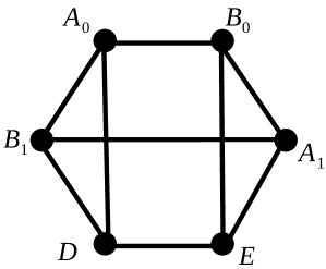
Figure 1: Compatibility graph associated with the contextuality scenario of the inequality given by Eq. (2.3).

For a box $P(c_{i}|C_{i})=\{p(c_{i}|C_{i})\}$ arising in the scenario in Fig. 1, the probability distributions are denoted as $p(a_{0}b_{0}|A_{0}B_{0})$ and $p(a_{1}b_{1}|A_{1}B_{1})$ in case of the contexts $C_{0}$ and $C_{3}$, respectively, $p(de|DE)$ in case of the context $C_{4}$ and $p(a_{0}b_{1}d|A_{0}B_{1}D)$ and $p(a_{1}b_{0}e|A_{1}B_{0}E)$ in case of the contexts $C_{1}$ and $C_{2}$, respectively. Here $a_{l},b_{m}\in\{0,1\}$, $\forall l,m\in\{0,1\}$ and $d,e\in\{0,1\}$. $D$ and $E$ are a joint measurement acting jointly on two subspaces. For instance, in the case of the set of observables given by Eq. (17), the observables $D$ and $E$ can be realized using a nonlocal gate followed by a Pauli measurement as in Ref. [56] or implementing joint projectors corresponding to these observables as in Ref. [57].

For the scenario whose compatibility graph is Fig. 1, to demonstrate quantum contextuality in an experimental setup, Cabello et. al. [6] considered the following noncontextuality inequality:

$$\braket{A_{0}B_{0}} +\braket{A_{0}B_{1}D}+\braket{A_{1}B_{0}E}+\braket{A_{1}B_{1}}$$

$$-\braket{DE}\leq 3,$$ (21)

where each term in the left-hand-side (LHS) is an expectation of the value of the joint measurement of the observables in each context such as $\braket{A_{0}B_{0}}=\sum_{a_{0},b_{0}}(-1)^{a_{0}\oplus b_{0}}p(a_{0}b_{0}|C_{0})$. Consider the contextual box $P_{P}(c_{i}|C_{i})$ arising from the state $\ket{\psi^{\texttt{me}}_{2}}$ for observables given by Eq. (17). This box has the following distributions:

$$P_{P}(c_{i}|C_{i})=\begin{dcases}\frac{1}{2},&\text{if }a_{0}+b_{0}=0\quad\texttt{for}\quad C_{0}\\ \frac{1}{4},&\text{if }a_{0}+b_{1}+d=0\quad\texttt{for}\quad C_{1}\\ \frac{1}{4},&\text{if }a_{1}+b_{0}+e=0\quad\texttt{for}\quad C_{2}\\ \frac{1}{2},&\text{if }a_{1}+b_{1}=0\quad\texttt{for}\quad C_{3}\\ \frac{1}{2},&\text{if }d+e=1\quad\texttt{for}\quad C_{4}\\ 0,&\texttt{otherwise}.\\ \end{dcases}$$ (22)

We call this box Peres box. The maximal violation $5$ of the inequality (2.3) is achieved by the Peres box ($P_{P}(c_{i}|C_{i})$ ). The Peres box (22), which is an extremal contextual box, is given by (according to the matrix notation provided in the Appendix. LABEL:matrixNota):

$$P_{P}(c_{i}|C_{i}) =\begin{pmatrix}\frac{1}{2}&0&0&\frac{1}{2}\\ \\[1.42271pt] \frac{1}{4}&0&0&\frac{1}{4}&0&\frac{1}{4}&\frac{1}{4}&0\\ \\[1.42271pt] \frac{1}{4}&0&0&\frac{1}{4}&0&\frac{1}{4}&\frac{1}{4}&0\\ \\[1.42271pt] \frac{1}{2}&0&0&\frac{1}{2}\\ \\[1.42271pt] 0&\frac{1}{2}&\frac{1}{2}&0\\ \end{pmatrix}$$ (23)

Based on contextual boxes that imply logical paradoxes, a notion called “strong contextuality" was formalized, see Sec. IV. A. 4 in Ref. [2]. Such a notion is characterized as having a measure of contextuality called the contextual fraction, $0\leq 1-\alpha\leq 1$, to take its maximal value $1$ [58]. The contextual fraction is obtained from the noncontextual fraction or noncontextual content [59, 60], $\alpha$, analogous to the quantity “local fraction" in Bell nonlocality [61] in the context of no-signaling boxes [62].

We consider the measure of contextuality called “contextuality cost" [51], related to the above measure. It is defined as

$$C(P) :=\texttt{inf}\{p\in[0,1]:P=pP_{C}+(1-p)P_{NC}\},$$ (24)

where infimum is the overall possible decomposition of the box into a mixture of some noncontextual box and some contextual box which may be quantum or non-quantum. The Popescu-Rohrlich box [63] is an example of a nonquantum box [54] that has $C(P)=1$ implying maximal contextuality. On the other hand, the Peres box (22) also has $C(P)=1$ while it is quantum.

3 Contextuality in the Peres’ scenario

We analyse in which range a one-parameter family of correlations arising in the scenario of Fig. 1 is contextual. This family of correlations is the noisy Peres box $P_{nP}(c_{i}|C_{i})$, given by

$$P_{nP}(c_{i}|C_{i}) =WP_{P}(c_{i}|C_{i})+(1-W)P_{N}(c_{i}|C_{i}),$$ (25)

with $0\leq W\leq 1$, where $P_{P}(c_{i}|C_{i})$ is the Peres box given by Eq. (22) and $P_{N}(c_{i}|C_{i})$ is a noncontextual box given by

$$P_{N}(c_{i}|C_{i})=\begin{dcases}\frac{1}{4},&\forall c_{i}\quad\texttt{for}\quad C_{0},C_{3},C_{4}\\ \frac{1}{4},&a_{0}+b_{1}+e=0\quad\texttt{for}\quad C_{1}\\ \frac{1}{4},&a_{1}+b_{0}+e=0\quad\texttt{for}\quad C_{2}\\ 0,&\texttt{otherwise}.\\ \end{dcases}$$ (26)

The noisy Peres box can be produced quantum-mechanically by two-qubit Werner state given (5) for the observables given by Eq. (17). The one-parameter family of states is entangled iff $W>1/3$ [49] and has a nonzero quantum discord for any $W>0$ [41, 42].

The noisy Peres box violates the noncontextuality inequality (2.3) for $W>1/3$, implying contextuality in the range $1/3<W\leq 1$. On the other hand, for $0<W\leq 1/3$ too, it does not have a noncontextual hidden variable model. This has been checked by finding out that it cannot be written as a convex mixture of the deterministic boxes in Appendix A for any $W>0$. For instance, consider the noisy Peres box (25) for $W=1/3$ (adapting the notation in Appendix. LABEL:matrixNota) given by

$$P^{W=1/3}_{nP}(c_{i}|C_{i}) :=\begin{pmatrix}\frac{1}{3}&\frac{1}{6}&\frac{1}{6}&\frac{1}{3}\\ \\[1.42271pt] \frac{1}{4}&0&0&\frac{1}{4}&0&\frac{1}{4}&\frac{1}{4}&0\\ \\[1.42271pt] \frac{1}{4}&0&0&\frac{1}{4}&0&\frac{1}{4}&\frac{1}{4}&0\\ \\[1.42271pt] \frac{1}{3}&\frac{1}{6}&\frac{1}{6}&\frac{1}{3}\\ \\[1.42271pt] \frac{1}{6}&\frac{1}{3}&\frac{1}{3}&\frac{1}{6}\\ \end{pmatrix}.$$ (27)

It can be checked that the above box cannot be written as a convex mixture of the deterministic boxes in the Appendix A (see Appendix. B for the proof). On the other hand, for $W=0$, the box can be written as the uniform mixture of four noncontextual deterministic boxes as follows:

$$P_{N} =\frac{1}{4}\Big{(}P^{(0000)(00)}_{D}+P^{(0110)(10)}_{D}+P^{(0111)(01)}_{D}$$ (28)

$$+P^{(0001)(11)}_{D}\Big{)},$$

where the deterministic boxes are given in the Appendix A. From the above considerations, we can now state the following observation:

Observation 1.

The noisy Peres box $P_{nP}(c_{i}|C_{i})$ given by Eq. (25) is contextual for $0<W\leq 1$ and has the contextuality cost $C(P)=W$.

It follows from this that the entanglement of the two-qubit state producing the box having contextual correlations is not necessary. Specifically, this is the case when it does not violate the noncontextuality inequality (2.3).

It may be noted that in Ref. [64], following the approach of Peres [46] directly, the impossibility of noncontextual value assignments was argued for the two-qubit Werner state for any nonzero discord. On the other hand, our approach is based on characterizing the box arising from the Werner state in terms of the extremal boxes.

The separable two-qubit states which have a nonzero discord in the Werner state family have superlocality in the context of the Bell scenario with two-input and two-output for each subsystem with local boxes having minimum hidden variable dimension $4$ [35, 37]. We now consider a box that can be produced from a two-qubit state which demonstrates superlocality in the above-mentioned Bell scenario with a lower amount, i.e., with a local box with minimum hidden variable dimension $3$. The following separable state has a rank of $2$:

$$\rho^{\texttt{rank}-2}_{\texttt{QQ}}=\frac{1}{2}\left(|00\rangle\langle 00|+|++\rangle\langle++|\right),$$ (29)

where $\ket{+}$ is the $+1$ eigenstate of the Pauli observable $X$, demonstrates superlocality with a local box (as in Eq. ($42$) of Ref. [37]) having the minimal $d_{\lambda}=3$.

Consider the box arising from the two-qubit state (29) for the observables given by Eq. (17). This box is given by,

$$P(c_{i}|C_{i}) =\begin{pmatrix}\frac{5}{8}&\frac{1}{8}&\frac{1}{8}&\frac{1}{8}\\ \\[1.42271pt] \frac{1}{2}&0&0&0&0&\frac{1}{4}&\frac{1}{4}&0\\ \\[1.42271pt] \frac{1}{2}&0&0&0&0&\frac{1}{4}&\frac{1}{4}&0\\ \\[1.42271pt] \frac{5}{8}&\frac{1}{8}&\frac{1}{8}&\frac{1}{8}\\ \\[1.42271pt] \frac{1}{4}&\frac{1}{4}&\frac{1}{4}&\frac{1}{4}\\ \end{pmatrix}.$$ (30)

The above box is noncontextual as it has a noncontextual deterministic model as follows:

$$P =\frac{1}{8}\Big{(}2P^{(0000)(00)}+P^{(0010)(10)}+P^{(0011)(01)}$$ (31)

$$+P^{(1000)(01)}+P^{(1010)(11)}+P^{(1100)(10)}$$

$$+P^{(1111)(11)}\Big{)}.$$

We are now going to consider a box arising from a rank-$3$ separable state given by

$$\rho^{\texttt{rank}-3}_{\texttt{QQ}} =\frac{1}{3}\Big{(}|00\rangle\langle 00|+|++\rangle\langle++|$$

$$+|+^{\prime}+^{\prime}\rangle\langle+^{\prime}+^{\prime}|\Big{)}.$$ (32)

Here $\ket{+^{\prime}}$ is the $+$ eigenstate of the Pauli observables $Y_{2}$. Quantum correlations in the above rank $2$ and rank $3$ states can be distinguished by the simultaneous correlations in MUBs, $Q_{2}$ and $Q_{3}$, [47]. The basis that can be used to quantify the classical correlations in these two states can be chosen to be that of $Z_{2}$. While the rank-$2$ state has the correlation in the basis of $X_{2}$ which is mutually unbiased to that of $Z_{2}$, the correlation in the third basis, i.e., that of $Y_{2}$, which is mutually unbiased to that of $X_{2}$ vanishes, whereas, the rank-$3$ state has the correlation in both of the two bases which are mutually unbiased to $Z_{2}$. This implies that the rank-$2$ state has $Q_{2}>0$ and $Q_{3}=0$, whereas, the rank-$3$ state has $Q_{2}>0$ as well as $Q_{3}>0$.

The box arising from the rank-$3$ state (3) for the observables given by Eq. (17) is contextual. This box is given by

$$P(c_{i}|C_{i}) =\begin{pmatrix}\frac{1}{2}&\frac{1}{6}&\frac{1}{6}&\frac{1}{6}\\ \\[1.42271pt] \frac{5}{12}&0&0&\frac{1}{12}&0&\frac{1}{4}&\frac{1}{4}&0\\ \\[1.42271pt] \frac{5}{12}&0&0&\frac{1}{12}&0&\frac{1}{4}&\frac{1}{4}&0\\ \\[1.42271pt] \frac{1}{2}&\frac{1}{6}&\frac{1}{6}&\frac{1}{6}\\ \\[1.42271pt] \frac{1}{6}&\frac{1}{3}&\frac{1}{3}&\frac{1}{6}\\ \end{pmatrix}.$$ (33)

It has been checked that the above box cannot be written as a convex mixture of the noncontextual deterministic boxes. The box (33) can be decomposed in terms of the extremal contextual box and a noncontextual box as follows:

$$P(c_{i}|C_{i})=\frac{1}{3}P_{P}(c_{i}|C_{i})+\frac{2}{3}P_{nc}(c_{i}|C_{i}),$$ (34)

where

$$P_{nc}(c_{i}|C_{i}) =\begin{pmatrix}\frac{1}{2}&\frac{1}{4}&\frac{1}{4}&0\\ \\[1.42271pt] \frac{1}{2}&0&0&0&0&\frac{1}{4}&\frac{1}{4}&0\\ \\[1.42271pt] \frac{1}{2}&0&0&0&0&\frac{1}{4}&\frac{1}{4}&0\\ \\[1.42271pt] \frac{1}{2}&\frac{1}{4}&\frac{1}{4}&0\\ \\[1.42271pt] \frac{1}{4}&\frac{1}{4}&\frac{1}{4}&\frac{1}{4}\\ \end{pmatrix},$$ (35)

implying that the box has the contextuality cost $C(P)=1/3$.

Note that the marginal correlations $\{p(a_{x}b_{y}|A_{x}B_{y})\}$, with $x,y=0,1$, of the box (25) correspond to the family of superlocal boxes studied in Ref. [37] (given by Eq. (32)), on the other hand, the marginal correlations $\{p(a_{x}b_{y}|A_{x}B_{y})\}$, of the box (35), also corresponds to a superlocal box having the minimal $d_{\lambda}=4$ (see Appendix. C for an LHV model of the box with $d_{\lambda}=4$). We have now obtained the following observation.

Observation 2.

The noisy Peres box $P_{nP}(c_{i}|C_{i})$ given by Eq. (25) having the contextuality cost $0<C(P)\leq 1/3$ and the contextual box $P(c_{i}|C_{i})$ given by Eq. (33) which has the contextuality cost $C(P)=1/3$ detects superlocal states with $d_{\lambda}=4$. On the other hand, there exist superlocal states with the minimal $d_{\lambda}=3$ that do not produce a contextual box. The superlocal states that produce a contextual box have the simultaneous correlations in MUBs [47] as $Q_{2}>0$ and $Q_{3}>0$, on the other hand, the superlocal states that do not produce a contextual box have $Q_{2}>0$, but $Q_{3}=0$.

From the above observations, we have now obtained the following main result.

Theorem 1.

Superlocality is necessary but not sufficient for producing a contextual box in the state-dependent scenario of Peres.

Proof.

Consider the marginal correlations $\{p(a_{x}b_{y}|A_{x}B_{y})\}$ of a box in the Peres’ scenario. Considering these marginal correlations as a bipartite NS box, if it is local and not superlocal, it can be produced using an LHV model of the minimal $d_{\lambda}\leq 2$ while quantum mechanically having a realization with a two-qubit system. It follows from our analysis that such sublocal correlations of two-qubit states cannot be used to demonstrate contextuality. The two-qubit states that do not have superlocality have zero discord in at least one way. Correlations in such a zero-discord state always lead to a noncontextual box. Also, if correlations in a nonzero discord state lead to a sublocal box which has no superlocality, such a sublocal box cannot be used to imply contextuality. As superlocality necessarily implies a nonzero discord both the ways and sublocal correlations of two-qubit states cannot be used to produce a contextual box, it follows that superlocality is necessary for producing a contextual box. On the other hand, there exists a superlocal state such as the state given by Eq. (29) which cannot lead to contextuality. This implies that superlocality is not sufficient for producing a contextual box. ∎

4 Supernoncontextuality

As in the Bell scenarios, in the context of observing a non-contextual box using a finite amount of noncontextual hidden variable [65], a quantum advantage can be identified in terms of supernoncontextuality. In a contextuality scenario, supernoncontextuality is defined as follows:

Definition 2.

Suppose we have a quantum state in $\mathbb{C}^{d_{Q}}$ and a set of contexts $\{C_{i}\}$ which produce a non-contextual box $P(c_{i}|C_{i})$ := $\{p(c_{i}|C_{i})\}_{c_{i},C_{i}}$. Then, supernoncontextuality holds iff there is no decomposition of the box in the form,

$$p(c_{i}|C_{i})=\sum^{d_{\lambda}-1}_{\lambda=0}p(\lambda)p(c_{i}|C_{i},\lambda)\hskip 8.5359pt\forall c,C_{i},$$ (36)

with dimension of the hidden variable $d_{\lambda}\leq$ $d^{g}_{Q}$. Here $\sum_{\lambda}p(\lambda)=1$, $P(c_{i}|C_{i},\lambda)$ := $\{p(c_{i}|C_{i},\lambda)\}_{c_{i},C_{i}}$ denotes an arbitrary non-contextual boxes for the given $\lambda$ ($\lambda$ occurs with probability $p(\lambda)$).

In the following, we present examples of supernoncontextuality in the Peres’ scenario.

4.1 Supernoncontextuality in the Peres’ scenario

Let us now start by providing an example of supernoncontextuality with the maximally entangled state $\ket{\psi^{\texttt{me}}_{2}}$ that can produce the Peres box. To this end, we consider the following choice of observables:

$$\begin{split}&A_{0}=Z_{2}\otimes\mathbbm{1}_{2},\quad B_{0}=\mathbbm{1}_{2}\otimes Z_{2},\\ &B_{1}=\mathbbm{1}_{2}\otimes X_{2},\quad A_{1}=X_{2}\otimes\mathbbm{1}_{2},\\ &D=\mathbbm{1}_{2}\otimes X_{2},\quad E=X_{2}\otimes\mathbbm{1}_{2}.\end{split}$$ (37)

In the above choice of observables, we do not invoke a nonlocal observable for $D$ and $E$ as used for the demonstration of contextuality. This also creates the above choice of observables to have less incompatibility than in the case of the observables (17) as there is no incompatibility between $D$ and $A_{1}$ and $E$ and $B_{1}$ in Eq. (37).

For the observables given above, the box produced from the two-qubit state $\ket{\psi^{\texttt{me}}_{2}}$ is noncontextual and is given by

$$P_{snc}(c_{i}|C_{i}) =\begin{pmatrix}\frac{1}{2}&0&0&\frac{1}{2}\\ \\[1.42271pt] \frac{1}{8}&\frac{1}{8}&\frac{1}{8}&\frac{1}{8}&\frac{1}{8}&\frac{1}{8}&\frac{1}{8}&\frac{1}{8}\\ \\[1.42271pt] \frac{1}{8}&\frac{1}{8}&\frac{1}{8}&\frac{1}{8}&\frac{1}{8}&\frac{1}{8}&\frac{1}{8}&\frac{1}{8}\\ \\[1.42271pt] \frac{1}{2}&0&0&\frac{1}{2}\\ \\[1.42271pt] \frac{1}{2}&0&0&\frac{1}{2}\\ \end{pmatrix}$$ (38)

The box given above has the following noncontextual deterministic model:

$$P_{snc}$$

$$=\frac{1}{8}\Big{(}P^{(0000)(00)}_{D}+P^{(0101)(00)}_{D}+P^{(1010)(00)}_{D}$$ (39)

$$+P^{(1111)(00)}_{D}+P^{(0000)(11)}_{D}+P^{(0101)(11)}_{D}$$

$$+P^{(1010)(11)}_{D}+P^{(1111)(11)}_{D}\Big{)}.$$

The simulation of the box using the deterministic boxes requires the $8$ deterministic boxes as appearing in the above decomposition, which implies the following noncontextual model:

$$P(c_{i}|C_{i}) =\sum^{d_{\lambda}-1}_{\lambda=0}p(\lambda)P(c_{i}|C_{i},\lambda),$$ (40)

with the dimension of the hidden variable $d_{\lambda}=8$. Here $P(c_{i}|C_{i},\lambda)=\{p(c_{i}|C_{i},\lambda)\}_{c_{i},C_{i}}$ are the deterministic boxes appearing in Eq. (4.1), respectively. From the above noncontexual model, it follows that the box is supernoncontextual since $d_{\lambda}=8>d_{Q}$ and this value of $d_{\lambda}$ is the minimal overall possible noncontextual hidden variable models. Similarly, supernoncontextuality of the Werner state family (5) and contextual state (3) can be demonstrated. We now state the following observation.

Observation 3.

Supernoncontextuality of the contextual states in Peres’ scenario occurs due to superlocality and not employing nonlocal measurements as in the case of demonstration of contextuality.

It may be checked that supernoncontextuality can also be demonstrated for the superlocal state (29) without invoking nonlocal observables.

In Observation. 2, we have seen that there are superlocal states which can lead to contextuality and certain superlocal states having lower superlocality in terms of the minimal $d_{\lambda}$ cannot lead to contextuality. In the following, we demonstrate examples of supernoncontextuality for such a noncontextual state employing incompatible measurements having nonlocal measurements. To this end, we consider the noncontextual box given by Eq. (30) which arises from the superlocal state (3) for the observables given by Eq. (17). This box, however, has the correlations that imply supernoncontextuality as we illustrate below.

For the box (30), from the decomposition of the box in terms of the deterministic boxes as given by Eq. (31), we have obtained the following noncontextual hidden variable model:

$$P(c_{i}|C_{i}) =\sum^{d_{\lambda}-1}_{\lambda=0}p(\lambda)P(c_{i}|C_{i},\lambda),$$ (41)

with the dimension of the hidden variable $d_{\lambda}=7$. Here $\sum_{\lambda}p(\lambda)=1$, $P(c|C_{i},\lambda)$ = $\{p(c|C_{i},\lambda)\}_{c,C_{i}}$ denotes a non-contextual box for the given $\lambda$ as in Eq. (31) ($\lambda$ occurs with probability $p(\lambda)=1/4$ for $\lambda=0,1$ and $p(\lambda)=1/8$, otherwise). It has been checked that the simulation of the box using the noncontextual deterministic boxes requires the above-mentioned seven deterministic boxes. This implies that the box has the minimal $d_{\lambda}=7$. Therefore, we have obtained the following observation.

Observation 4.

The box $P(c_{i}|C_{i})$ given by Eq. (30) is supernoncontextual. In other words, the box requires a hidden variable of dimension $d_{\lambda}=7$ to be simulated using a noncontextual hidden variable model, on the other hand, it can be simulated quantum mechanically using a quantum system with global Hilbert space dimension $d^{g}_{Q}=4$.

We now proceed to provide our next example of supernoncontextuality for which the quantum simulation of the box demonstrating supernoncontextuality does not require a superlocal state. Before that, we provide an example of a noncontextual box that arises from a classically-correlated state for incompatible measurements given by Eq. (17), but has no supernoncontextuality. Let us consider the following noncontextual box:

$$P(c_{i}|C_{i}) =\begin{pmatrix}\frac{1}{2}&0&0&\frac{1}{2}\\ \\[1.42271pt] \frac{1}{4}&0&0&\frac{1}{4}&0&\frac{1}{4}&\frac{1}{4}&0\\ \\[1.42271pt] \frac{1}{4}&0&0&\frac{1}{4}&0&\frac{1}{4}&\frac{1}{4}&0\\ \\[1.42271pt] \frac{1}{4}&\frac{1}{4}&\frac{1}{4}&\frac{1}{4}\\ \\[1.42271pt] \frac{1}{4}&\frac{1}{4}&\frac{1}{4}&\frac{1}{4}\\ \end{pmatrix}$$ (42)

which can be produced using the CC state $\rho_{\texttt{CC}}$ given by Eq. (7) for the observables given by Eq. (17). The above box (42) can be reproduced using a noncontextual hidden variable model with $d_{\lambda}=4$ as follows:

$$P(c_{i}|C_{i}) =\sum^{3}_{\lambda=0}p(\lambda)P(c_{i}|C_{i},\lambda).$$ (43)

Here $\sum_{\lambda}p(\lambda)=1$, $P(c|C_{i},\lambda)$ = $\{p(c_{i}|C_{i},\lambda)\}_{c_{i},C_{i}}$ denotes a deterministic non-contextual box for the given $\lambda$ given by $P(c_{i}|C_{i},0)=P^{(0000)(00)}_{D}$, $P(c_{i}|C_{i},1)=P^{(0111)(10)}_{D}$, $P(c_{i}|C_{i},2)=P^{(1101)(01)}_{D}$ and $P(c_{i}|C_{i},3)=P^{(1010)(11)}_{D}$ are the deterministic boxes given in Appendix LABEL:matrixNota. ($\lambda$ occurs with probability $p(\lambda)=\frac{1}{4}$, $\forall$ $\lambda$).

In the above example of a noncontextual box which has the minimal $d_{\lambda}=4$, correlations are present in the three contexts $C_{0}$, $C_{1}$ and $C_{2}$. We now proceed to provide another example of a noncontextual box arising from the classically-correlated state (7), but having supernoncontextuality. In this example, the number of contexts having correlations is increased to the four contexts $C_{0}$, $C_{1}$, $C_{2}$ and $C_{3}$. This is achieved by invoking the following choice of observables:

$$\begin{split}&A_{0}=\frac{Z_{2}+X_{2}}{\sqrt{2}}\otimes\mathbbm{1}_{2},\quad B_{0}=\mathbbm{1}_{2}\otimes\frac{Z_{2}+X_{2}}{\sqrt{2}},\\ &B_{1}=\mathbbm{1}_{2}\otimes\frac{Z_{2}-X_{2}}{\sqrt{2}},\quad A_{1}=\frac{Z_{2}-X_{2}}{\sqrt{2}}\otimes\mathbbm{1}_{2},\\ &D=\frac{Z_{2}+X_{2}}{\sqrt{2}}\otimes\frac{Z_{2}-X_{2}}{\sqrt{2}},\quad E=\frac{Z_{2}-X_{2}}{\sqrt{2}}\otimes\frac{Z_{2}+X_{2}}{\sqrt{2}}.\end{split}$$ (44)

For this choice of observables, we obtain the following noncontextual box:

$$P(c_{i}|C_{i}) =\begin{pmatrix}\frac{3}{8}&\frac{1}{8}&\frac{1}{8}&\frac{3}{8}\\ \\[1.42271pt] \frac{3}{8}&0&0&\frac{3}{8}&0&\frac{1}{8}&\frac{1}{8}&0\\ \\[1.42271pt] \frac{3}{8}&0&0&\frac{3}{8}&0&\frac{1}{8}&\frac{1}{8}&0\\ \\[1.42271pt] \frac{3}{8}&\frac{1}{8}&\frac{1}{8}&\frac{3}{8}\\ \\[1.42271pt] \frac{1}{2}&\frac{1}{4}&\frac{1}{4}&0\\ \end{pmatrix}$$ (45)

The above box can be decomposed in terms of the noncontextual deterministic boxes in more than one way. Out of these models, we present the following model which provides a noncontextual hidden variable model with $d_{\lambda}$ minimized. The box (45) has the following noncontextual deterministic hidden variable model:

$$P(c_{i}|C_{i}) =\sum^{d_{\lambda}-1}_{\lambda=0}p(\lambda)P(c_{i}|C_{i},\lambda),$$ (46)

with dimension of the hidden variable $d_{\lambda}=6$. Here $\sum_{\lambda}p(\lambda)=1$, $P(c|C_{i},\lambda)$ := $\{p(c_{i}|C_{i},\lambda)\}_{c_{i},C_{i}}$ denotes a deterministic non-contextual box for the given $\lambda$ given by $P(c_{i}|C_{i},0)=P^{(0000)(00)}_{D}$, $P(c_{i}|C_{i},1)=P^{(0101)(00)}_{D}$, $P(c_{i}|C_{i},2)=P^{(0010)(10)}_{D}$, $P(c_{i}|C_{i},3)=P^{(0111)(10)}_{D}$, $P(c_{i}|C_{i},4)=P^{(0011)(01)}_{D}$ and $P(c_{i}|C_{i},5)=P^{(0110)(01)}_{D}$, are the deterministic boxes given in Appendix LABEL:matrixNota ($\lambda$ occurs with probability $p(\lambda)=\frac{1}{4}$, for $\lambda=0,1$ and $p(\lambda)=\frac{1}{8}$, otherwise). We have now obtained the following observation.

Observation 5.

The box $P(c_{i}|C_{i})$ given by Eq. (45) is supernoncontextual. In other words, the box requires a hidden variable of dimension $d_{\lambda}=6$ to be simulated using a noncontextual hidden variable model, on the other hand, it can be simulated quantum mechanically using a quantum system with lower global Hilbert space dimension $d^{g}_{Q}=4$. Supernoncontextuality of the box (45) as quantified by $d_{\lambda}$ is lower than that of the box (30).

We now identify the resources present in two-qubit states leading to supernoncontextuality in the above two examples. We note that in the case of box given by Eq. (30), the marginal correlations $\{p(a_{x}b_{y}|A_{x}B_{y})\}$ correspond to a superlocal box (given Eq. (42) in Ref. [37]) that detects a superlocal state with the minimal $d_{\lambda}=3$. We have now obtained the following observation.

Observation 6.

The box (30) detects a noncontextual state which has superlocality with the minimal $d_{\lambda}=3$. Such superlocal states have the simultaneous correlations in MUBs [47] as $Q_{2}>0$ and $Q_{3}=0$.

In the case of the box given by Eq. (45), the marginal correlations $\{p(a_{x}b_{y}|A_{x}B_{y})\}$ correspond to a local box that detects quantum correlation of the two-qubit state (7) due to the simultaneous correlations in two MUBs $C_{2}$ [48] . These bases are that of the observables in the set $\left\{\frac{Z_{2}+X_{2}}{\sqrt{2}},\frac{Z_{2}-X_{2}}{\sqrt{2}}\right\}$. Thus, the nonzero $C_{2}$ of the two-qubit state acts as a resource of supernoncontextuality of the box (45) since it arises invoking incompatible measurements as in Eq. (44) that contain the mutually unbiased basis in each qubit subspace giving rising to the nonzero $C_{2}$. We have now obtained the following observation.

Observation 7.

While the occurrence of supernoncontextuality does not require a superlocal state, supernoncontextuality of the box (45) arises due to quantum correlation beyond discord of the two-qubit state as captured by the simultaneous correlations in two MUBs ($C_{2}>0$) [48].

5 Quantum correlation beyond contextuality in Peres’ scenario

State	Quantum correlation	Resource used
$\rho_{W}$ (5)	Contextuality cost $C(P)=W$ (25)	Superlocality with $d_{\lambda}=4$ ($Q_{2}>0$ and $Q_{3}>0$)
		and correlations due to nonlocal measurements
$\rho^{\texttt{rank}-3}_{\texttt{QQ}}$ (3)	Contextuality cost $C(P)=\frac{1}{3}$ (33)	Superlocality with $d_{\lambda}=4$ ($Q_{2}>0$ and $Q_{3}>0$)
		and correlations due to nonlocal measurements
$\rho^{\texttt{rank}-2}_{\texttt{QQ}}$ (29)	Supernoncontextual (30), $d_{\lambda}=7>d_{Q}$	Superlocality with $d_{\lambda}=3$ ($Q_{2}>0$ and $Q_{3}=0$)
		and correlations due to nonlocal measurements
$\rho_{CC}$ (7)	Supernoncontextual (45), $d_{\lambda}=6>d_{Q}$	Quantum correlation due to nonzero $C_{2}$
		and correlations due to nonlocal measurements

Table 1: Summary of the results concerning quantum correlations of the boxes arising from the two-qubit states considered in this work. The states given by Eqs. (5) and (3) have a nonzero contextuality cost $C(P)$, while the states (29) and (7) do not produce a contextual box, but have supernoncontextuality with the minimal $d_{\lambda}=7,6$, respectively. For the states that have a nonzero contextuality cost, superlocality with $d_{\lambda}=4$ and correlations in nonlocal measurements are used to imply contextuality. Such states have simultaneous correlations in two and three MUBs as indicated by a nonzero $Q_{2}$ and $Q_{3}$, respectively. For the states that have supernoncontextuality with $d_{\lambda}=7$, the lower amount of superlocality, i.e., superlocal correlations with $d_{\lambda}=3$ is used to imply supernoncontextual correlations. For such states, the simultaneous correlations in third MUBs, i.e., $Q_{3}$, vanishes. For the states that demonstrate supernoncontextuality with the lower amount of the hidden variable dimension, i.e., $d_{\lambda}=6$, quantum correlation beyond discord, i.e., the simultaneous correlations in general two MUBs $C_{2}$ and correlations in nonlocal measurements act as a resource. See also Fig. 2 for a different hierarchy of correlations in separable states that we have identified in this work.

It has been checked that the sublocal state (42) cannot lead to supernoncontextuality if nonlocal measurements are not employed in the incompatible measurements giving rising to the given box, even if quantum correlation due to the nonzero $C_{2}$ is used. For instance, employing the following choice of observables:

$$\begin{split}&A_{0}=\frac{Z_{2}+X_{2}}{\sqrt{2}}\otimes\mathbbm{1}_{2},\quad B_{0}=\mathbbm{1}_{2}\otimes\frac{Z_{2}+X_{2}}{\sqrt{2}},\\ &B_{1}=\mathbbm{1}_{2}\otimes\frac{Z_{2}-X_{2}}{\sqrt{2}},\quad A_{1}=\frac{Z_{2}-X_{2}}{\sqrt{2}}\otimes\mathbbm{1}_{2},\\ &D=\mathbbm{1}_{2}\otimes\frac{Z_{2}-X_{2}}{\sqrt{2}},\quad E=\frac{Z_{2}-X_{2}}{\sqrt{2}}\otimes\mathbbm{1}_{2},\end{split}$$ (47)

the CC state (7) produces a noncontextual box, whose marginal correlations $\{p(a_{x}b_{y}|A_{x}B_{y})\}$ detects the simultaneous correlations due to the nonzero $C_{2}$, has a noncontextual hidden variable model with $d_{\lambda}=4$. Note that the above choice of observables has less incompatibility than in the case of (44).

The above observation leads us to formulate a notion of nonclassicality which we refer to as ‘quantum correlation beyond contextuality’ based on supernoncontextuality for noncontextual boxes that implies the presence of nonlocal observables. This notion is defined as follows.

Definition 3.

Suppose we have a quantum state in $\mathbb{C}^{d_{Q}}$ and a set of measurements of the contexts $\{C_{i}\}$ of the Peres’ scenario, which produce a box $P(c_{i}|C_{i})$. Then, the box implies the presence of quantum correlations iff there is no decomposition of the box in the form,

$$p(c_{i}|C_{i})=\sum^{d_{\lambda}-1}_{\lambda=0}p(\lambda)p(c_{i}|C_{i},\lambda)\hskip 8.5359pt\forall c_{i},C_{i},$$ (48)

with the dimension of the hidden variable $d_{\lambda}\leq$ $d^{g}_{Q}$, provided that the box detects incompatible measurements having nonlocal observables for $D$ and $E$.

We now provide the following observation in the context of the above definition.

Observation 8.

Contextual boxes in the Peres’ scenario satisfy the condition of quantum correlation in Def. 3. On the other hand, from this definition, it follows that quantum correlation beyond contextuality is present in the boxes (30) and $(\ref{cc2qhd})$, whereas, the noncontextual boxes arising from superlocal states with the minimal $d_{\lambda}=4$, such as the box given by Eq. (38), do not have such form of quantum correlation though they exhibit supernoncontextuality.

In Table. 1, we have summarized the results of quantum correlation in the context of the boxes studied in this work.

Figure 2: The regions $I$-$VII$ represent the convex set of correlations in separable two-qubit states. The regions $VI$ and $VII$ denote the superlocal correlations that imply superlocality with the minimal $d_{\lambda}=4$. Within such correlations that have a simultaneous correlation in two and three mutually unbiased bases, i.e., $Q_{2}>0$ and $Q_{3}>0$, the region $VI$ denotes the contextual correlations. On the other hand, the regions $IV$ and $V$ denote the superlocal correlations that imply superlocality with the minimal $d_{\lambda}=3$. Within such correlations that have the simultaneous correlations only in two mutually unbiased bases, i.e., $Q_{2}>0$ and $Q_{3}=0$, the region $IV$ denotes the supernoncontextual correlations with the minimal $d_{\lambda}=7$ that imply quantum correlation beyond contextuality. The region $V$ has noncontextual correlations that may have a minimal $d_{\lambda}\geq 7$. Whereas, the regions $I$-$III$ denote sublocal correlations that have the minimal $d_{\lambda}=2$ and a different form of simultaneous correlations in mutually unbiased bases, i.e., $C_{2}>0$. Within such sublocal correlations, the regions $II$-$III$ denote the noncontextual correlations with a minimal $d_{\lambda}\geq 6$. Within such noncontextual correlations, the region $II$ denotes the supernoncontextual correlations with the minimal $d_{\lambda}=6$ that imply quantum correlation beyond contextuality. Whereas the region $I$ denotes the subnoncontextual correlations with a minimal $d_{\lambda}\leq 5$.

Based on the above observations in the context of supernoncontextuality, we have obtained our second main result.

Theorem 2.

For quantum correlation based on supernoncontextuality, superlocality is neither sufficient and is nor necessary.

Proof.

There exist superlocal correlations leading to supernoncontextuality that do not imply the presence of full incompatibility of measurements with nonlocal observables in the set of contexts. For instance, consider the supernoncontextual box given by Eq. (38). This box which implies the presence of superlocality does not imply the presence of full incompatibility with nonlocal observables. On the other hand, there exists sublocal states which lead to supernoncontextuality such as the box given by Eq. (45). Such supernoncontextuality also implies the presence of full incompatibility of measurements with nonlocal observables. ∎

6 Conclusions and Discussions

In this work, we have characterized contextuality of certain classes of two-qubit states in the scenario of the Peres’ proof of contextuality [46], which has the five contexts as in Fig. 1. To this end, we have adopted the framework of boxes in the contextuality scenarios to the above-mentioned scenario. We have characterized the contextuality of certain classes of boxes arising from the two-qubit states having different types of quantum correlations. While entanglement of the two-qubit states is not necessary to imply contextuality in the state-dependent scenario, we have identified which types of quantum correlations in the two-qubit states lead to contextuality. We have demonstrated the superlocality of certain two-qubit states in the two-input and two-output Bell scenario with the minimal hidden variable dimension $4$ can be used to demonstrate contextuality. On the other hand, we demonstrate that the superlocality of the two-qubit states is not sufficient for producing a contextual box as there are superlocal states with the lower minimal hidden variable dimension, i.e., $3$, which cannot be used to demonstrate contextuality. We also identify that the simultaneous correlations in both two and three MUBs as captured by $Q_{2}$ and $Q_{3}$ defined in [47] have to be present in the superlocal states to observe contextuality.

We have considered supernoncontextuality as an extension of superlocality to contextuality scenarios. Supernoncontextuality indicates a quantum advantage in using a quantum system of lower Hilbert space dimension to simulate the box over the requirement of high dimensionality of the hidden variable required to simulate it using a noncontextual hidden variable model. Based on such a quantum advantage, a different notion of nonclassicality, which we refer to as ‘quantum correlation beyond quantum contextuality’, can be identified. In one of our examples of quantum correlation based on supernoncontextuality in the context of the scenario in Fig. 1, we have demonstrated that superlocality with the minimal hidden variable dimension $3$ which does not demonstrate contextuality acts as a resource. In our other example, we have demonstrated that superlocality is not necessary for supernoncontextuality, but it arises from quantum correlation beyond discord of the two-qubit state as indicated by the simultaneous correlations in two mutually unbiased bases ($C_{2}>0$) [48] and correlations due to nonlocal measurements.

Bell nonlocality of a bipartite state in the context of the given Bell scenario may be interpreted as quantum correlation due to the two-way discordant correlation present in the state while employing a certain choice of incompatible measurements on each subsystem. The set of quantum correlations of two-way discordant states, however, forms a nonconvex superset of the set of all quantum correlations that have Bell nonlocality in the given Bell scenario. The condition that the boxes that do not imply Bell nonlocality lead to a subset of boxes that have the convexity property [34]. In this convex set of boxes, there exists a subset of the boxes within the two-way discordant correlations that imply quantum correlation based on superlocality [35]. The complement of this set which has the boxes which are neither Bell nonlocal nor superlocal is, however, not convex.

Analogous to the above characterization of NS boxes, the contextuality of the ND boxes in the scenario studied in this work arises due to the two-way discordant correlations of the two-qubit states employing certain choices of measurements having incompatibility between different contexts and nonlocal observables. The condition of contextuality identifies a nonconvex subset of the boxes that require a nonzero discord implying superlocality to be simulated, while the complement of this set has the convexity property. Within this convex set of boxes that do not demonstrate contextuality, there exists a nonconvex subset of boxes that imply supernoncontextuality. Bell nonlocality of quantum correlations necessarily requires a strong form of quantum correlation in the state, i.e., a nonzero discord in both ways with entanglement. Whereas, the contextuality of the scenario studied in this work does not require the presence of entanglement either in the two-qubit state or in the measurements.

Superlocality of quantum correlations requires a nonzero discord both ways, whereas, supernoncontextuality of quantum correlations of the scenario studied in this work does not require such a form of quantum correlation, but arises due to a different aspect of quantum correlation of the two-qubit states. From the perspective that quantum correlation in contextuality scenarios arises due to a certain choice of incompatible measurements [50], the quantum correlation of the scenario studied in this work may be interpreted as quantum correlation originating from the simultaneous correlations in the incompatible bases that are present in any nonproduct state and correlations in nonlocal measurements.

Acknowledgement.– C. J. would like to thank Dr Ashutosh Rai, Dr Jaskaran Singh, Dr Debarshi Das and Dr Wei-Min Zhang for useful discussions and the National Science and Technology Council (formerly Ministry of Science and Technology), Taiwan (Grant No. MOST 111-2811-M-006-040-MY2). RS acknowledges with thanks the partial support by the Indian Science & Engineering Research Board (SERB grant CRG/2022/008345).

Appendix A Noncontextual deterministic boxes of the scenario in Fig. 1

Let us denote the ND boxes $P(c_{i}|C_{i})$ of the contextuality scenario with the compatibility graph as shown in Fig. 1 in the matrix form as follows:

The scenario has $64$ extremal noncontextual boxes which are deterministic boxes denoted as $P^{(\alpha\beta\gamma\epsilon)(de)}_{D}$, with $\alpha,\beta,\gamma,\epsilon\in\{0,1\}$. $P^{\alpha\beta\gamma\epsilon}_{D}(a_{x}b_{y}|A_{x}B_{y})$ denote the marginal deterministic boxes of $P^{(\alpha\beta\gamma\epsilon)(de)}_{D}$. $P^{\alpha\beta\gamma\epsilon}_{D}(a_{x}b_{y}|A_{x}B_{y})$ are given by

$$P_{D}^{\alpha\beta\gamma\epsilon}(a_{x}b_{y}|A_{x}B_{y})=\begin{dcases}1,&\text{if }a_{x}=\alpha x\oplus\beta,b_{y}=\gamma y\oplus\epsilon\\ 0,&\text{otherwise},\end{dcases}$$ (49)

in matrix form, the above boxes are given by

$$P_{D}^{0000}=\begin{pmatrix}1&0&0&0\\ 1&0&0&0\\ 1&0&0&0\\ 1&0&0&0\\ \end{pmatrix};\leavevmode\nobreak\ \leavevmode\nobreak\ \leavevmode\nobreak\ P_{D}^{0001}=\begin{pmatrix}0&1&0&0\\ 0&1&0&0\\ 0&1&0&0\\ 0&1&0&0\\ \end{pmatrix};\leavevmode\nobreak\ \leavevmode\nobreak\ \leavevmode\nobreak\ P_{D}^{0010}=\begin{pmatrix}1&0&0&0\\ 0&1&0&0\\ 1&0&0&0\\ 0&1&0&0\\ \end{pmatrix};\leavevmode\nobreak\ \leavevmode\nobreak\ \leavevmode\nobreak\ P_{D}^{0011}=\begin{pmatrix}0&1&0&0\\ 1&0&0&0\\ 0&1&0&0\\ 1&0&0&0\\ \end{pmatrix};$$

$$P_{D}^{0100}=\begin{pmatrix}0&0&1&0\\ 0&0&1&0\\ 0&0&1&0\\ 0&0&1&0\\ \end{pmatrix};\leavevmode\nobreak\ \leavevmode\nobreak\ \leavevmode\nobreak\ P_{D}^{0101}=\begin{pmatrix}0&0&0&1\\ 0&0&0&1\\ 0&0&0&1\\ 0&0&0&1\\ \end{pmatrix};\leavevmode\nobreak\ \leavevmode\nobreak\ \leavevmode\nobreak\ P_{D}^{0110}=\begin{pmatrix}0&0&1&0\\ 0&0&0&1\\ 0&0&1&0\\ 0&0&0&1\\ \end{pmatrix};\leavevmode\nobreak\ \leavevmode\nobreak\ \leavevmode\nobreak\ P_{D}^{0111}=\begin{pmatrix}0&0&0&1\\ 0&0&1&0\\ 0&0&0&1\\ 0&0&1&0\\ \end{pmatrix};$$

$$P_{D}^{1000}=\begin{pmatrix}1&0&0&0\\ 1&0&0&0\\ 0&0&1&0\\ 0&0&1&0\\ \end{pmatrix};\leavevmode\nobreak\ \leavevmode\nobreak\ \leavevmode\nobreak\ P_{D}^{1001}=\begin{pmatrix}0&1&0&0\\ 0&1&0&0\\ 0&0&0&1\\ 0&0&0&1\\ \end{pmatrix};\leavevmode\nobreak\ \leavevmode\nobreak\ \leavevmode\nobreak\ P_{D}^{1010}=\begin{pmatrix}1&0&0&0\\ 0&1&0&0\\ 0&0&1&0\\ 0&0&0&1\\ \end{pmatrix};\leavevmode\nobreak\ \leavevmode\nobreak\ \leavevmode\nobreak\ P_{D}^{1011}=\begin{pmatrix}0&1&0&0\\ 1&0&0&0\\ 0&0&0&1\\ 0&0&1&0\\ \end{pmatrix};$$

$$P_{D}^{1100}=\begin{pmatrix}0&0&1&0\\ 0&0&1&0\\ 1&0&0&0\\ 1&0&0&0\\ \end{pmatrix};\leavevmode\nobreak\ \leavevmode\nobreak\ \leavevmode\nobreak\ P_{D}^{1101}=\begin{pmatrix}0&0&0&1\\ 0&0&0&1\\ 0&1&0&0\\ 0&1&0&0\\ \end{pmatrix};\leavevmode\nobreak\ \leavevmode\nobreak\ \leavevmode\nobreak\ P_{D}^{1110}=\begin{pmatrix}0&0&1&0\\ 0&0&0&1\\ 1&0&0&0\\ 0&1&0&0\\ \end{pmatrix};\leavevmode\nobreak\ \leavevmode\nobreak\ \leavevmode\nobreak\ P_{D}^{1111}=\begin{pmatrix}0&0&0&1\\ 0&0&1&0\\ 0&1&0&0\\ 1&0&0&0\\ \end{pmatrix}$$

The probability $p_{D}(00|DE)$ takes the value $1$ if $de=00$ in $P^{(\alpha\beta\gamma\epsilon)(de)}_{D}$. Using the above mentioned notations, the $16$ deterministic boxes $P^{(\alpha\beta\gamma\epsilon)(00)}_{D}$ are given in the matrix form as follows:

respectively, the $16$ deterministic boxes for $de=10$ in $P^{(\alpha\beta\gamma\epsilon)(de)}_{D}$ are given as follows:

respectively, the $16$ deterministic boxes for $de=01$ in $P^{(\alpha\beta\gamma\epsilon)(de)}_{D}$ are given as follows:

and, finally, the $16$ deterministic boxes for $de=11$ in $P^{(\alpha\beta\gamma\epsilon)(de)}_{D}$ are given as follows:

respectively.

Appendix B Contextuality of the box (27)

There are $16$ deterministic boxes that satisfy the zero probabilities of the box (27). Any convex mixture of these boxes given by

$$P =p_{1}P^{0000(00)}_{D}+p_{2}P^{0101(00)}_{D}+p_{3}P^{1011(00)}_{D}+p_{4}P^{1110(00)}_{D}$$

$$+p_{5}P^{0010(10)}_{D}+p_{6}P^{0111(10)}_{D}+p_{7}P^{1001(10)}_{D}+p_{8}P^{1100(10)}_{D}$$

$$+p_{9}P^{0011(01)}_{D}+p_{10}P^{0110(01)}_{D}+p_{11}P^{1000(01)}_{D}+p_{12}P^{1101(01)}_{D}$$

$$+p_{13}P^{0001(11)}_{D}+p_{14}P^{0100(11)}_{D}+p_{15}P^{1010(11)}_{D}+p_{16}P^{1111(11)}_{D},$$ (50)

has the zero probabilities of the box (27). To check the contextuality of the box (27), it suffices to show if there are no weights, $0\leq p_{i}\leq 1$, with $i=1,2\cdots 16$ and $\sum_{i}p_{i}=1$, in the above decomposition to produce all other nonzero probabilities of the box (27). Using such a decomposition, it has been checked that it is either possible to reproduce only the probabilities in rows $1$ to $4$ of the box (27), i.e., a noncontextual box given by

$$P(c_{i}|C_{i}) =\frac{1}{6}P^{0000(00)}_{D}+\frac{1}{6}P^{0101(00)}_{D}+\frac{1}{12}P^{1011(00)}_{D}+\frac{1}{12}P^{1110(00)}_{D}$$

$$+\frac{1}{12}P^{0001(11)}_{D}+\frac{1}{12}P^{0100(11)}_{D}+\frac{1}{6}P^{1010(11)}_{D}+\frac{1}{6}P^{1111(11)}_{D}$$

$$=\begin{pmatrix}\frac{1}{3}&\frac{1}{6}&\frac{1}{6}&\frac{1}{3}\\ \\[1.42271pt] \frac{1}{4}&0&0&\frac{1}{4}&0&\frac{1}{4}&\frac{1}{4}&0\\ \\[1.42271pt] \frac{1}{4}&0&0&\frac{1}{4}&0&\frac{1}{4}&\frac{1}{4}&0\\ \\[1.42271pt] \frac{1}{3}&\frac{1}{6}&\frac{1}{6}&\frac{1}{3}\\ \\[1.42271pt] \frac{1}{2}&0&0&\frac{1}{2}\\ \end{pmatrix},$$ (51)

is obtained or only the probabilities in rows except for the row $1$ or $4$ i.e., a noncontextual box given by

$$P(c_{i}|C_{i}) =\frac{1}{6}\left(\frac{1}{3}P^{0000(00)}_{D}+\frac{1}{3}P^{0101(00)}_{D}+\frac{1}{6}P^{1011(00)}_{D}+\frac{1}{6}P^{1110(00)}_{D}\right)$$

$$+\frac{1}{3}\left(\frac{1}{3}P^{0010(10)}_{D}+\frac{1}{3}P^{0111(10)}_{D}+\frac{1}{6}P^{1001(10)}_{D}+\frac{1}{6}P^{1100(10)}_{D}\right)$$

$$+\frac{1}{3}\left(\frac{1}{6}P^{0011(01)}_{D}+\frac{1}{6}P^{0110(01)}_{D}+\frac{1}{3}P^{1000(01)}_{D}+\frac{1}{3}P^{1101(01)}_{D}\right)$$

$$+\frac{1}{6}\left(\frac{1}{6}P^{0001(11)}_{D}+\frac{1}{6}P^{0100(11)}_{D}+\frac{1}{3}P^{1010(11)}_{D}+\frac{1}{3}P^{1111(11)}_{D}\right)$$

$$:=\begin{pmatrix}\frac{1}{3}&\frac{1}{6}&\frac{1}{6}&\frac{1}{3}\\ \\[1.42271pt] \frac{1}{4}&0&0&\frac{1}{4}&0&\frac{1}{4}&\frac{1}{4}&0\\ \\[1.42271pt] \frac{1}{4}&0&0&\frac{1}{4}&0&\frac{1}{4}&\frac{1}{4}&0\\ \\[1.42271pt] \frac{2}{9}&\frac{5}{18}&\frac{5}{18}&\frac{2}{9}\\ \\[1.42271pt] \frac{1}{6}&\frac{1}{3}&\frac{1}{3}&\frac{1}{6}\\ \end{pmatrix},$$ (52)

or the following noncontextual box:

$$P(c_{i}|C_{i}) =\frac{1}{6}\left(\frac{1}{3}P^{0000(00)}_{D}+\frac{1}{3}P^{0101(00)}_{D}+\frac{1}{6}P^{1011(00)}_{D}+\frac{1}{6}P^{1110(00)}_{D}\right)$$

$$+\frac{1}{3}\left(\frac{1}{6}P^{0010(10)}_{D}+\frac{1}{6}P^{0111(10)}_{D}+\frac{1}{3}P^{1001(10)}_{D}+\frac{1}{3}P^{1100(10)}_{D}\right)$$

$$+\frac{1}{3}\left(\frac{1}{3}P^{0011(01)}_{D}+\frac{1}{3}P^{0110(01)}_{D}+\frac{1}{6}P^{1000(01)}_{D}+\frac{1}{6}P^{1101(01)}_{D}\right)$$

$$+\frac{1}{6}\left(\frac{1}{6}P^{0001(11)}_{D}+\frac{1}{6}P^{0100(11)}_{D}+\frac{1}{3}P^{1010(11)}_{D}+\frac{1}{3}P^{1111(11)}_{D}\right)$$

$$=\begin{pmatrix}\frac{2}{9}&\frac{5}{18}&\frac{5}{18}&\frac{2}{9}\\ \\[1.42271pt] \frac{1}{4}&0&0&\frac{1}{4}&0&\frac{1}{4}&\frac{1}{4}&0\\ \\[1.42271pt] \frac{1}{4}&0&0&\frac{1}{4}&0&\frac{1}{4}&\frac{1}{4}&0\\ \\[1.42271pt] \frac{1}{3}&\frac{1}{6}&\frac{1}{6}&\frac{1}{3}\\ \\[1.42271pt] \frac{1}{6}&\frac{1}{3}&\frac{1}{3}&\frac{1}{6}\\ \end{pmatrix},$$ (53)

respectively, is obtained. It then follows that the box is contextual as it does not admit a decomposition in terms of the noncontextual deterministic boxes.

Appendix C LHV model with the minimal dimension for the marginal local box of the contextual box (33)

Consider the marginal correlations $\{p(a_{x}b_{y}|A_{x}B_{y})\}$ of the box given by (33). These marginal correlations correspond to a superlocal box given by

$$P(a_{x}b_{y}|A_{x}B_{y})=\begin{pmatrix}\frac{1}{2}\quad&\frac{1}{6}\quad&\frac{1}{6}\quad&\frac{1}{6}\\ \\[1.42271pt] \frac{5}{12}\quad&\frac{1}{4}\quad&\frac{1}{4}\quad&\frac{1}{12}\\ \\[1.42271pt] \frac{5}{12}\quad&\frac{1}{4}\quad&\frac{1}{4}\quad&\frac{1}{12}\\ \\[1.42271pt] \frac{1}{2}\quad&\frac{1}{6}\quad&\frac{1}{6}\quad&\frac{1}{6}\\ \end{pmatrix}.\leavevmode\nobreak\ \leavevmode\nobreak\ \leavevmode\nobreak\$$ (54)

The above local box can be written in terms of the deterministic boxes given by (49) as follows:

$$P(a_{x}b_{y}|A_{x}B_{y}) =\frac{1}{12}\Big{(}3P^{0000}_{D}+2P^{0010}_{D}+2P^{0011}_{D}+2P^{0100}_{D}$$

$$+P^{0101}_{D}+P^{1010}_{D}+P^{1111}_{D}\Big{)}.$$ (55)

From the above decomposition, we now obtain the following LHV model of the box by letting nondeterministic outcomes for Bob’s observables:

$$P(a_{x}b_{y}|A_{x}B_{y}) =\sum^{3}_{\lambda=0}p(\lambda)P(a_{x}|A_{x},\lambda)P_{\lambda}(b_{y}|B_{y},\lambda),$$ (56)

where Alice’s strategies $P(a_{x}|A_{x},\lambda)$ are given by $P(a_{x}|A_{x},\lambda=0)=P^{00}_{D}(a_{x}|A_{x})$, $P(a_{x}|A_{x},\lambda=1)=P^{01}_{D}(a_{x}|A_{x})$, $P(a_{x}|A_{x},\lambda=2)=P^{10}_{D}(a_{x}|A_{x})$ and $P(a_{x}|A_{x},\lambda=3)=P^{11}_{D}(a_{x}|A_{x})$, on the other hand, Bob’s strategies $P(b_{y}|B_{y},\lambda)$ are given by

$$P(b_{y}|b_{y},\lambda=0)=\frac{3P^{00}_{D}(b_{x}|B_{y})+2P^{10}_{D}(b_{x}|B_{y})+2P^{11}_{D}(b_{x}|B_{y})}{7},$$

$P(b_{y}|B_{y},\lambda=1)=\frac{2P^{00}_{D}(b_{y}|B_{y})+P^{01}_{D}(b_{y}|B_{y})}{3}$, $P(b_{y}|B_{y},\lambda=2)=P^{10}_{D}(b_{y}|B_{y})$ and $P(b_{y}|B_{y},\lambda=3)=P^{11}_{D}(b_{y}|B_{y})$, which have nondeterministic outcomes for $\lambda=0,1$. The above LHV model also minimizes the dimension of the hidden variable overall possible LHV models for the box. This may be checked by adopting the approach taken in Ref. [37].

References

• [1] Nicolas Brunner, Daniel Cavalcanti, Stefano Pironio, Valerio Scarani, and Stephanie Wehner. “Bell nonlocality”. Rev. Mod. Phys. 86, 419–478 (2014).
• [2] Costantino Budroni, Adán Cabello, Otfried Gühne, Matthias Kleinmann, and Jan-Åke Larsson. “Kochen-specker contextuality”. Rev. Mod. Phys. 94, 045007 (2022).
• [3] John S. Bell. “On the problem of hidden variables in quantum mechanics”. Rev. Mod. Phys. 38, 447–452 (1966).
• [4] J. S. Bell. “On the einstein podolsky rosen paradox”. Physics Physique Fizika 1, 195–200 (1964).
• [5] Simon Kochen and E. P. Specker. “The problem of hidden variables in quantum mechanics”. Journal of Mathematics and Mechanics 17, 59–87 (1967). url: http://www.jstor.org/stable/24902153.
• [6] Adán Cabello, Stefan Filipp, Helmut Rauch, and Yuji Hasegawa. “Proposed experiment for testing quantum contextuality with neutrons”. Phys. Rev. Lett. 100, 130404 (2008).
• [7] Adán Cabello. “Experimentally testable state-independent quantum contextuality”. Phys. Rev. Lett. 101, 210401 (2008).
• [8] Alexander A. Klyachko, M. Ali Can, Sinem Binicioğlu, and Alexander S. Shumovsky. “Simple test for hidden variables in spin-1 systems”. Phys. Rev. Lett. 101, 020403 (2008).
• [9] Jonathan Barrett, Lucien Hardy, and Adrian Kent. “No signaling and quantum key distribution”. Phys. Rev. Lett. 95, 010503 (2005).
• [10] Antonio Acín, Nicolas Gisin, and Lluis Masanes. “From bell’s theorem to secure quantum key distribution”. Phys. Rev. Lett. 97, 120405 (2006).
• [11] S. Pironio, A. Acín, S. Massar, A. Boyer de la Giroday, D. N. Matsukevich, P. Maunz, S. Olmschenk, D. Hayes, L. Luo, T. A. Manning, and C. Monroe. “Random numbers certified by bell’s theorem”. Nature 464, 1021 (2010).
• [12] Antonio Acín, Nicolas Brunner, Nicolas Gisin, Serge Massar, Stefano Pironio, and Valerio Scarani. “Device-independent security of quantum cryptography against collective attacks”. Phys. Rev. Lett. 98, 230501 (2007).
• [13] Antonio Acín and Lluis Masanes. “Certified randomness in quantum physics”. Nature 540, 213–219 (2016).
• [14] Marcin Pawłowski and Marek Żukowski. “Entanglement-assisted random access codes”. Phys. Rev. A 81, 042326 (2010).
• [15] Andrzej Grudka, Karol Horodecki, Michał Horodecki, Waldemar Kłobus, and Marcin Pawłowski. “When are popescu-rohrlich boxes and random access codes equivalent?”. Phys. Rev. Lett. 113, 100401 (2014).
• [16] Armin Tavakoli, Breno Marques, Marcin Pawłowski, and Mohamed Bourennane. “Spatial versus sequential correlations for random access coding”. Phys. Rev. A 93, 032336 (2016).
• [17] Dominic Mayers and Andrew Yao. “Self testing quantum apparatus”. Quantum Inf. Comput. 4, 273 (2004).
• [18] Pavel Sekatski, Jean-Daniel Bancal, Sebastian Wagner, and Nicolas Sangouard. “Certifying the building blocks of quantum computers from bell’s theorem”. Phys. Rev. Lett. 121, 180505 (2018).
• [19] Ivan Šupić and Joseph Bowles. “Self-testing of quantum systems: a review”. Quantum 4, 337 (2020).
• [20] Janet Anders and Dan E. Browne. “Computational power of correlations”. Phys. Rev. Lett. 102, 050502 (2009).
• [21] Adán Cabello, Vincenzo D’Ambrosio, Eleonora Nagali, and Fabio Sciarrino. “Hybrid ququart-encoded quantum cryptography protected by kochen-specker contextuality”. Phys. Rev. A 84, 030302 (2011).
• [22] Juan Bermejo-Vega, Nicolas Delfosse, Dan E. Browne, Cihan Okay, and Robert Raussendorf. “Contextuality as a resource for models of quantum computation with qubits”. Phys. Rev. Lett. 119, 120505 (2017).
• [23] Jaskaran Singh, Kishor Bharti, and Arvind. “Quantum key distribution protocol based on contextuality monogamy”. Phys. Rev. A 95, 062333 (2017).
• [24] Debashis Saha, Paweł Horodecki, and Marcin Pawłowski. “State independent contextuality advances one-way communication”. New Journal of Physics 21, 093057 (2019).
• [25] Kishor Bharti, Maharshi Ray, Antonios Varvitsiotis, Naqueeb Ahmad Warsi, Adán Cabello, and Leong-Chuan Kwek. “Robust self-testing of quantum systems via noncontextuality inequalities”. Phys. Rev. Lett. 122, 250403 (2019).
• [26] Kishor Bharti, Maharshi Ray, Antonios Varvitsiotis, Adán Cabello, and Leong-Chuan Kwek. “Local certification of programmable quantum devices of arbitrary high dimensionality” (2019). arXiv:1911.09448.
• [27] Abu Ashik Md. Irfan, Karl Mayer, Gerardo Ortiz, and Emanuel Knill. “Certified quantum measurement of majorana fermions”. Phys. Rev. A 101, 032106 (2020).
• [28] Debashis Saha, Rafael Santos, and Remigiusz Augusiak. “Sum-of-squares decompositions for a family of noncontextuality inequalities and self-testing of quantum devices”. Quantum 4, 302 (2020).
• [29] Xiao-Min Hu, Yi Xie, Atul Singh Arora, Ming-Zhong Ai, Kishor Bharti, Jie Zhang, Wei Wu, Ping-Xing Chen, Jin-Ming Cui, Bi-Heng Liu, Yun-Feng Huang, Chuan-Feng Li, Guang-Can Guo, Jérémie Roland, Adán Cabello, and Leong-Chuan Kwek. “Self-testing of a single quantum system: Theory and experiment”. npj Quantum Inf 9, 103 (2022).
• [30] Rafael Santos, Chellasamy Jebarathinam, and Remigiusz Augusiak. “Scalable noncontextuality inequalities and certification of multiqubit quantum systems”. Phys. Rev. A 106, 012431 (2022).
• [31] Chellasamy Jebarathinam, Gautam Sharma, Sk Sazim, and Remigiusz Augusiak. “Certification of two-qubit quantum systems with temporal non-contextuality inequality” (2023). arXiv:2307.06710.
• [32] Mark Howard, Joel Wallman, Victor Veitch, and Joseph Emerson. “Contextuality supplies the ‘magic’ for quantum computation”. Nature 510, 351 (2014).
• [33] Matty J. Hoban, Joel J. Wallman, Hussain Anwar, Naïri Usher, Robert Raussendorf, and Dan E. Browne. “Measurement-based classical computation”. Phys. Rev. Lett. 112, 140505 (2014).
• [34] John Matthew Donohue and Elie Wolfe. “Identifying nonconvexity in the sets of limited-dimension quantum correlations”. Phys. Rev. A 92, 062120 (2015).
• [35] C. Jebaratnam, S. Aravinda, and R. Srikanth. “Nonclassicality of local bipartite correlations”. Phys. Rev. A 95, 032120 (2017).
• [36] C Jebaratnam, Debarshi Das, Suchetana Goswami, R Srikanth, and A S Majumdar. “Operational nonclassicality of local multipartite correlations in the limited-dimensional simulation scenario”. J. Phys. A: Math. Theor. 51, 365304 (2018). url: http://stacks.iop.org/1751-8121/51/i=36/a=365304.
• [37] Debarshi Das, Bihalan Bhattacharya, Chandan Datta, Arup Roy, C. Jebaratnam, A. S. Majumdar, and R. Srikanth. “Operational characterization of quantumness of unsteerable bipartite states”. Phys. Rev. A 97, 062335 (2018).
• [38] Chellasamy Jebarathinam, Debarshi Das, and R. Srikanth. “Asymmetric one-sided semi-device-independent steerability of quantum discordant states”. Phys. Rev. A 108, 042211 (2023).
• [39] H. M. Wiseman, S. J. Jones, and A. C. Doherty. “Steering, entanglement, nonlocality, and the einstein-podolsky-rosen paradox”. Phys. Rev. Lett. 98, 140402 (2007).
• [40] Roope Uola, Ana C. S. Costa, H. Chau Nguyen, and Otfried Gühne. “Quantum steering”. Rev. Mod. Phys. 92, 015001 (2020).
• [41] Harold Ollivier and Wojciech H. Zurek. “Quantum discord: A measure of the quantumness of correlations”. Phys. Rev. Lett. 88, 017901 (2001).
• [42] L. Henderson and V. Vedral. “Classical, quantum and total correlations”. J. Phys. A 34, 6899 (2001). url: http://stacks.iop.org/0305-4470/34/i=35/a=315.
• [43] K. T. Goh, J.-D. Bancal, and V. Scarani. “Measurement-device-independent quantification of entanglement for given hilbert space dimension”. New J. Phys. 18, 045022 (2016). url: http://iopscience.iop.org/article/10.1088/1367-2630/18/4/045022.
• [44] C. Jebarathinam, Debarshi Das, Som Kanjilal, R. Srikanth, Debasis Sarkar, Indrani Chattopadhyay, and A. S. Majumdar. “Superunsteerability as a quantifiable resource for random access codes assisted by bell-diagonal states”. Phys. Rev. A 100, 012344 (2019).
• [45] Chellasamy Jebarathinam and Debarshi Das. “Certifying quantumness beyond steering and nonlocality and its implications on quantum information processing”. Quantum Information and Computation 23, 379–401 (2023).
• [46] Asher Peres. “Incompatible results of quantum measurements”. Physics Letters A 151, 107–108 (1990).
• [47] Shengjun Wu, Zhihao Ma, Zhihua Chen, and Sixia Yu. “Reveal quantum correlation in complementary bases”. Scientific Reports 4, 4036 (2014).
• [48] Y Guo and S Wu. “Quantum correlation exists in any non-product state”. Sci. Rep 4, 7179 (2014).
• [49] Reinhard F. Werner. “Quantum states with einstein-podolsky-rosen correlations admitting a hidden-variable model”. Phys. Rev. A 40, 4277–4281 (1989).
• [50] Zhen-Peng Xu and Adán Cabello. “Necessary and sufficient condition for contextuality from incompatibility”. Phys. Rev. A 99, 020103 (2019).
• [51] A. Grudka, K. Horodecki, M. Horodecki, P. Horodecki, R. Horodecki, P. Joshi, W. Kłobus, and A. Wójcik. “Quantifying contextuality”. Phys. Rev. Lett. 112, 120401 (2014).
• [52] Barbara Amaral, Adán Cabello, Marcelo Terra Cunha, and Leandro Aolita. “Noncontextual wirings”. Phys. Rev. Lett. 120, 130403 (2018).
• [53] Karol Horodecki, Jingfang Zhou, Maciej Stankiewicz, Roberto Salazar, Paweł Horodecki, Robert Raussendorf, Ryszard Horodecki, Ravishankar Ramanathan, and Emily Tyhurst. “The rank of contextuality”. New Journal of Physics 25, 073003 (2023).
• [54] Mateus Araújo, Marco Túlio Quintino, Costantino Budroni, Marcelo Terra Cunha, and Adán Cabello. “All noncontextuality inequalities for the $n$-cycle scenario”. Phys. Rev. A 88, 022118 (2013).
• [55] N. David Mermin. “Simple unified form for the major no-hidden-variables theorems”. Phys. Rev. Lett. 65, 3373–3376 (1990).
• [56] Gerhard Kirchmair, Florian Zähringer, Rene Gerritsma, Matthias Kleinmann, Otfried Gühne, Adán Cabello, Rainer Blatt, and Christian F. Roos. “State-independent experimental test of quantum contextuality”. Nature 460, 494–497 (2009). url: https://doi.org/10.1038/nature08172.
• [57] Elias Amselem, Magnus Rådmark, Mohamed Bourennane, and Adán Cabello. “State-independent quantum contextuality with single photons”. Phys. Rev. Lett. 103, 160405 (2009).
• [58] Samson Abramsky, Rui Soares Barbosa, and Shane Mansfield. “Contextual fraction as a measure of contextuality”. Phys. Rev. Lett. 119, 050504 (2017).
• [59] Samson Abramsky and Adam Brandenburger. “The sheaf-theoretic structure of non-locality and contextuality”. New Journal of Physics 13, 113036 (2011).
• [60] Elias Amselem, Lars Eirik Danielsen, Antonio J. López-Tarrida, José R. Portillo, Mohamed Bourennane, and Adán Cabello. “Experimental fully contextual correlations”. Phys. Rev. Lett. 108, 200405 (2012).
• [61] Avshalom C. Elitzur, Sandu Popescu, and Daniel Rohrlich. “Quantum nonlocality for each pair in an ensemble”. Phys. Lett. A 162, 25 – 28 (1992).
• [62] Nicolas Brunner, Daniel Cavalcanti, Alejo Salles, and Paul Skrzypczyk. “Bound nonlocality and activation”. Phys. Rev. Lett. 106, 020402 (2011).
• [63] Sandu Popescu and Daniel Rohrlich. “Quantum nonlocality as an axiom”. Found. Phys. 24, 379–385 (1994).
• [64] Asma Al-Qasimi. “Contextuality and quantum discord”. Physics Letters A 449, 128347 (2022).
• [65] Nicholas M. Harrigan, Terry Rudolph, and Scott Aaronson. “Representing probabilistic data via ontological models” (2007). arXiv: Quantum Physics:0709.1149v2.