AFBT GAN: enhanced explainability and diagnostic performance for cognitive decline by counterfactual generative adversarial network

Abstract

Existing explanation results of functional connectivity (FC) are generally created by using classification result labels and correlation analysis methods such as Pearson’s correlation or gradient backward. However, the diagnostic model is still trained on the black box model and might lack the attention of FCs in important regions during the training. To enhance the explainability and improve diagnostic performance, providing prior knowledge on neurodegeneration-related regions when healthy subjects (HC) develop into subject cognitive decline (SCD) and mild cognitive impairment (MCI) for the diagnostic model is a key step. To better determine the neurodegeneration-related regions, we employ counterfactual reasoning to generate the target label FC matrices derived from source label FC and then subtract source label FC with target label FC. The counterfactual reasoning architecture is constructed by adaptive forward and backward transformer generative adversarial network (AFBT GAN), which is specifically designed by network property in FC and inverse patch embedding operation in the transformer. The specific design can make the model focus more on the current network correlation and employ the global insight of the transformer to reconstruct FC, which both help the generation of high-quality target label FC. The validation experiments are conducted on both clinical and public datasets, the generated attention map are both vital correlated to cognitive function and the diagnostic performance is also significant. The code is available at https://github.com/SXR3015/AFBT-GAN.

1 Introduction

Identifying mild cognitive impairment (MCI) and subject cognitive decline (SCD) is vital for the early intervention of Alzheimer’s disease. Functional connectivity (FC) changes at default mode network, frontal-parietal network at network level [1] and posterior cingulate cortex, left anterior insula at region level [2] have been used to distinguish HC and MCI in the clinical research. Since the development of machine learning, FC is widely used in the diagnostic model of MCI and SCD. Based on the FC, researchers have exploited many diagnostic models including convolution neural network-based [3], support vector machine-based [4], transformer-based [5]. However, to enhance the models’ explanation and show the models’ attention on the FC of the brain regions, only using these black box classification architectures is not enough.

To explain the model’s attention regions at brain functional connectivity, researchers have developed Pearson’s correlation test and cross-validation for searching the most discriminative correlations [6]. By selecting the highest frequency correlation in the cross-validation, the most discriminative correlations are decided. The other explanation methods are based on the gradient backward of the diagnostic model, including gradient [7] and activation map methods [8]. However, all these explained methods are estimated based on the classification result labels and are a static evaluation process, which might ignore the neurodegeneration information when HC develops into SCD or MCI. Inspired by this, constructing the diagnostic models’ prior attention regions based on neurodegeneration information is closer to clinical reality.

One of the methods to construct diagnostic models’ prior attention on neurodegeneration information is to generate counterfactual attention, which is built by counterfactual reasoning architecture. Although counterfactual reasoning hasn’t been used for FC in functional magnetic resonance imaging (fMRI), this method has been applied in structural magnetic resonance imaging (sMRI). Oh et al. generated the target label sMRI by adding the counterfactual map to the source label sMRI. The counterfactual map represents the sMRI changes when HC subjects develop into MCI [9]. Ren et al. also achieved a better performance by using counterfactual reasoning in the detection of brain disease [10]. However, applying counterfactual reasoning to FC is a harder problem because FC is a high-level imaging feature of fMRI and has a strong network property.

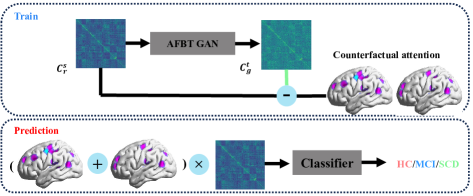
Figure 1: The framework of generated attention and prediction. By subtracting the generated target label FC (denoted as $C_{g}^{t}$ ) and true source label FC (denoted as $C_{r}^{s}$), the counterfactual attention of brain regions is defined. Then apply the counterfactual attention to FC to train a diagnostic model for prediction.

To improve the explainability and diagnostic performance of the diagnostic model based on FC, we build a counterfactual reasoning architecture. It directs the model’s attention to neurodegeneration-related regions within the FC, mimicking the neurodegeneration process by generating the target label FC from the source label FC. The main contributions of this paper are in the following:

• We propose counterfactual reasoning architecture for generating neurodegeneration-related regions map (called counterfactual attention) in the training stage and train a diagnostic model for prediction based on these regions.The architecture is shown in Fig. 1.

  • training stage: we design an adaptive forward and backward transformer generative adversarial network (AFBT GAN) to generate the target label FC. And then subtract the target label FC and source label FC to build counterfactual attention of all source labels.

  • prediction stage: By adding all counterfactual attention and applying the total attention map to FC, the diagnostic model receives an initial neurodegeneration region attention on the input FC. Then a new diagnostic model is trained.

• We propose an adaptive forward and backward transformer (AFBT) for reconstructing FC, which adaptively encodes and decodes the FC network by network. To provide global insight for encoding and decoding FC, the forward and backward process to encode and decode tokens is employed.

2 Method

2.1 Counterfactual generative adversarial network

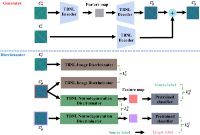
Figure 2: The main framework of AFBT GAN. The generator initially utilizes the noising source label input $C^{s}_{n}$ to reconstruct the source label FC and extract disease-related information from the mean target label FC $C^{t}_{r}$ of the dataset. Then it applies this information to the reconstructed source label FC to generate target label FC $C^{t}_{g}$ derived from the source label FC $C^{s}_{r}$. $C^{s}_{n}$ is created by adding noise to $C^{s}_{r}$. The discriminator employs image and neurodegeneration parts to ensure the $C^{t}_{g}$ has similar FC characteristics and different cognitive information from $C^{s}_{r}$.

2.1.1 Generator

The generator of AFBT GAN encodes the noise source label FC $C_{n}^{s}$ constructed by source label FC and Gaussian noise into the feature map. Then the feature map inputs the decoder to the AFBT decoder to reconstruct the source label FC $C_{g}^{s}$. Another AFBT encoder extracts the feature of the mean target label FC of the whole dataset (denoted as $C_{r}^{t}$), which is regarded as the disease-related information feature. Finally, the disease-related information feature is added to $C_{g}^{s}$ to generate $C_{g}^{t}$. The specific architecture of generator is shown in Fig. 2. To make the $C_{g}^{s}$ and $C_{g}^{t}$ more realistic to FC, the generator loss included perpetual loss $L_{p}$, generation loss $L_{g}$, and cross-entropy loss of label $L_{c}$. $L_{p}$ and $L_{g}$ ensure the $C_{g}^{s}$ has the same FC characteristic as $C_{r}^{s}$. $L_{c}$ guarantees the $C_{g}^{t}$ has the correct target label. The label of $C_{g}^{t}$ is created by a pre-trained classifier $CLS$. The total loss $L_{G}$ is in the following:

$$L_{p}=MSE\left(VGG\left(C_{g}^{s}\right),VGG\left(C_{r}^{s}\right)\right)$$ (1)

$$L_{gen}=MSE\left(C_{g}^{s},C_{r}^{s}\right)$$ (2)

$$L_{c}=CE\left(CLS\left(C_{g}^{t}\right),y_{t}\right)$$ (3)

$$L_{g}=L_{p}+L_{c}+L_{gen}\vspace{-2mm}$$ (4)

where $MSE$ represents the mean square error, $VGG$ represents VGG16 network, and $CE$ represents cross-entropy loss, $y_{t}$ represents the expected target label.

2.1.2 Discriminator

To ensure the generator generates the high-quality $C_{g}^{t}$ and $C_{g}^{s}$, the discriminator contains an AFBT image and AFBT neurodegeneration part. The architecture is shown in Fig. 2. The image part is designed to discriminate whether FC characteristics of $C_{g}^{s}$ are similar to the $C_{r}^{s}$, which loss is denoted as $l_{d}^{c}$. The neurodegeneration part is designed to make the discriminator learn the cognitive-decline-related feature from FC, which means the pre-trained classifier can classify different kinds of subjects based on these discriminative features. We design several losses to ensure the feature map extracted by the neurodegeneration part represents cognitive-decline-related information. The cross-entropy loss $l_{d}^{sl}$ is calculated between the diagnostic results of feature maps from $C_{g}^{s}$ and the source label. This ensures the neurodegeneration discriminator learns the same cognitive features from $C_{g}^{s}$ and $C_{r}^{s}$. The cross-entropy loss $l_{d}^{tl}$ is calculated between the diagnostic results of feature maps from $C_{g}^{t}$ and the target label. This ensures neurodegeneration discriminator learns the cognitive features of the target label. To ensure the discriminative feature map at the map level, the mean square error $l_{d}^{D}$ is computed between the feature map of $C_{g}^{s}$ and $C_{g}^{t}$. The loss $l_{D}$ of the generator is shown in the following equator:

$$l_{d}^{c}=mean\left(log\left(1-S\left(D_{i}\left(C_{g}^{s}\right)\right)\right)*log\left(S\left(D_{i}\left(C_{r}^{s}\right)\right)\right)\right)$$ (5)

$$l_{d}^{sl}=CE\left(CLS\left(D_{n}\left(C_{g}^{s}\right)\right),y_{s}\right)$$ (6)

$$l_{d}^{tl}=CE\left(CLS\left(D_{n}\left(C_{g}^{t}\right)\right),l_{t}\right)$$ (7)

$$l_{d}^{D}=mean\left(log\left(1-S\left(D_{i}\left(C_{g}^{s}\right)\right)\right)*log\left(1-S\left(D_{i}\left(C_{g}^{t}\right)\right)\right)\right)$$ (8)

$$L_{D}=l_{d}^{c}+l_{d}^{sl}+l_{d}^{tl}+l_{d}^{D}\vspace{-2mm}$$ (9)

where $D_{i}$ represents the image discriminator and $D_{n}$ represents the neurodegeneration discriminator, $y_{s}$ represents the source label.

2.2 Adaptive forward and backward transformer

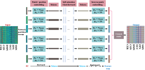
Figure 3: The detail of AFBT encoder. The patch embedding and inverse patch embedding are set according to the number of regions in the network, which is a forward and backward process. $p_{w}$ means patch width, $p_{h}$ means patch height, $n_{*}$ the number of regions in the network.

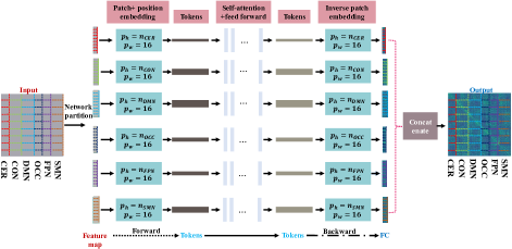
Figure 4: The detail of AFBT decoder. The input is a feature map, the output is an FC matrix.

Directly inputting the FC of all networks into the transformer block could result in equal attention across all regions. Inspired by vision transformer [11] and community-aware framework in fMRI [12], the basic block of AFBT is designed to adaptively focus on the current network correlation of FC. Otherwise, patch embedding is the forward process to encode the input (FC or feature map) into tokens, while inverse patch embedding is the backward process to decode the tokens into outputs ((FC or feature map). The combination of patch embedding and inverse patch embedding helps the model understand the current network correlation in both encoding and decoding. Firstly, the input FC is segmented into CER (cerebellum network), CON (cingulo-opercular network), DMN (default mode network), OCC (occipital network), FPN (frontoparietal network), and SMN (sensorimotor network). Then, at the patch embedding and position embedding step, the patch height is set as the number of regions in the network, and the patch width is set as 16. Later, the tokens generated from patch embedding and position embedding are fed into self-attention and feed-forward blocks, encoding them accordingly. Finally, to decode these tokens, the inverse patch embedding is designed to generate the feature map or FC. The existing encoding of the FC generation network is based on convolution network with a narrow insight [13]. The inverse patch embedding directly decodes the FC at the transformer with a global insight. The specific explanation is shown in 3 and 4. The formula of AFBT can defined in the following:

$$O=C\left(\tilde{P}_{i}\left(T_{i}\left(P_{i}\left(S_{i}\left(I\right)\right)\right)\right)\right)\vspace{-4mm}$$ (10)

where $I$ represents the input feature map or FC, $i$ rpresents $i$-th network of FC, $S_{i}$ represents network segmentation, $P_{i}$ reprents the patch embedding and position embedding operation, $T$ represents transformer block, $\tilde{P}_{i}$ represents inverse patch embedding, $C$ represents concentation operation.

3 Experiments and Results

3.1 Dataset and experiment setup

3.1.1 Dataset

In this paper, the hospital-collected data and Alzheimer’s Disease Neuroimaging Initiative (ADNI) data are used to train and validate the AFBT GAN. The hospital-collected data includes 58 individuals diagnosed with SCD, 89 individuals with MCI, and 67 individuals diagnosed with HC. ADNI data includes 22 individuals diagnosed with SCD, 67 individuals diagnosed with HC, and 95 individuals diagnosed with MCI. The data is pre-processed by SPM12 [19], steps including slice-timing correction, head motion estimation and correction, intra-subject registration, and co-registration.

3.1.2 Experiment setup

The depth of the transformer in the encoder and decoder generator is set as 3. The depth of the transformer in the image and neurodegeneration part is set as 8. The quantitation indices including accuracy (ACC), recall, precision, and F1-score (F1) are employed to evaluate the performance of the pre-trained and final classifier.

3.2 Results

3.2.1 Diagnostic performance

To validate the diagnostic performance, the baseline models are built on the following formula:

• $R_{*}$ means ResNet10 or ResNet18 [20]. $T*$ means the transformer has a different number of multi-head self-attention. ’B’ represents using 16 heads in the transformer, while ’L’ uses 32 heads, and ’S’ uses 8 heads. ’A’ means channel attention, the most generally used attention mechanism [21].

• $R_{*}//$ means the diagnostic model only constructed by ResNet. $R_{*}A$ means the diagnostic model is constructed by ResNet and channel attention. $R_{*}T*$ means the diagnostic model is constructed by ResNet and transformer.

Prposed method utilizes the architecture of ReseNet 10 and transformer with head number 16. The baseline model inputs FC directly, while the proposed method inputs FC masked by counterfactual attention. As shown in Tab. 1, the proposed method achieves better diagnostic performance in three tasks and two datasets.

Table 1: The diagnostic performance of binary diagnostic task (HC-SCD, HC-MCI, and MCI-SCD) on hospital-collected and ADNI datasets.

			Hospital				ADNI
			Acc	Recall	Precision	F1	Acc	Recall	Precision	F1
HC vsSCD	R10	//	0.8333	0.4667	1.0000	0.6364	0.6786	0.7823	0.6130	0.6874
		A	0.8667	0.6667	0.8000	0.7273	0.6905	0.8413	0.6033	0.7027
		T-S	0.8000	0.4000	0.8000	0.5333	0.6190	0.3764	0.6667	0.4812
		T-B	0.8000	0.4000	0.8000	0.5333	0.6667	0.6049	0.6627	0.6325
		T-L	0.8000	0.4000	0.8000	0.5333	0.6049	0.7078	0.5802	0.6377
	R18	//	0.8000	0.4000	0.8000	0.5333	0.6905	0.5510	0.6648	0.6026
		A	0.8000	0.4000	0.8000	0.5333	0.6310	0.3220	0.7143	0.4439
		T-S	0.8000	0.4000	0.8000	0.5333	0.6207	0.3739	0.6345	0.4705
		T-B	0.8000	0.5333	0.6800	0.5978	0.6543	0.3128	0.6614	0.4247
		T-L	0.8000	0.4000	0.8000	0.5333	0.6420	0.4815	0.6587	0.5563
	Proposed		0.9333	0.8667	1.0000	0.9286	0.7284	0.6667	0.7445	0.7035
HC vsMCI	R10	//	0.6552	0.9004	0.6552	0.7585	0.6562	0.8611	0.6456	0.7379
		A	0.6458	0.9167	0.6331	0.7490	0.6207	0.9632	0.6137	0.7497
		T-S	0.6437	0.8812	0.6381	0.7402	0.6146	0.8542	0.6102	0.7119
		T-B	0.6322	0.8084	0.6528	0.7223	0.6458	0.9514	0.6193	0.7502
		T-L	0.6667	0.9195	0.6468	0.7594	0.6465	0.8364	0.6505	0.7318
	R18	//	0.7126	0.9080	0.7125	0.7985	0.6667	0.6929	0.6729	0.6828
		A	0.7011	0.7739	0.7755	0.7747	0.6458	0.7986	0.6468	0.7147
		T-S	0.6782	0.8889	0.6629	0.7594	0.6458	0.8194	0.6610	0.7317
		T-B	0.6437	1.0000	0.6247	0.7690	0.6667	0.7847	0.6724	0.7242
		T-L	0.6207	0.8927	0.6243	0.7348	0.6354	0.6736	0.7037	0.6883
	Proposed		0.7471	0.9816	0.7056	0.8210	0.6970	0.8653	0.6709	0.7558
MCI vsSCD	R10	//	0.7778	0.9392	0.8133	0.8717	0.6989	0.7233	0.7610	0.7417
		A	0.8500	1.0000	0.8500	0.9189	0.6989	0.7247	0.7552	0.7396
		T-S	0.7692	1.0000	0.7692	0.8695	0.7204	0.7864	0.7935	0.7899
		T-B	0.7692	1.0000	0.7692	0.8695	0.6989	0.9541	0.6726	0.7890
		T-L	0.7949	1.0000	0.7857	0.8800	0.6989	0.8380	0.7097	0.7685
	R18	//	0.7949	1.0000	0.7857	0.8800	0.6774	0.9828	0.6523	0.7841
		A	0.8500	1.0000	0.8500	0.9189	0.7097	0.8165	0.7322	0.7721
		T-S	0.7692	1.0000	0.7692	0.8695	0.6989	0.8509	0.6943	0.7647
		T-B	0.8205	1.0000	0.8047	0.8918	0.6667	0.6344	0.7586	0.6910
		T-L	0.7692	1.0000	0.7692	0.8695	0.6882	0.9140	0.6779	0.7784
	Proposed		0.9487	0.9707	0.9615	0.9661	0.7312	0.8656	0.7307	0.7924

Table 2: The network of top 10 regions at the counterfactual attention in HC-MCI, HC-SCD, and MCI-SCD diagnostic task.

HC-SCD	HC	FPN	DMN	SMN	CON	OCC	SMN	OCC	CON	CER	FPN
	SCD	FPN	DMN	SMN	OCC	CON	SMN	FPN	CON	DMN	SMN
HC-MCI	HC	FPN	SMN	FPN	OCC	SMN	DMN	CER	OCC	DMN	FPN
	MCI	FPN	SMN	FPN	OCC	SMN	FPN	DMN	CON	CER	OCC
MCI-SCD	MCI	DMN	SMN	CON	DMN	FPN	DMN	FPN	CER	SMN	DMN
	SCD	FPN	DMN	CER	SMN	SMN	SMN	CON	DMN	CON	OCC

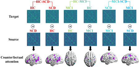
Figure 5: The generated target label FC and counterfactual attention in HC-MCI, HC-SCD and MCI-SCD diagnostic task.

3.2.2 Counterfactual attention map

At the neurodegeneration process of HC to MCI, there is a significant change in the FC of the prefrontal, cingulate, and hippocampus [14]. At the intervention of MCI, there is a significant change in the FC of cingulate and gyrus [15]. Therefore, during the conversion process of each binary diagnostic task, most of the attention regions should be the same but exist a little differently. In Fig. 5, the attention of each region in FC is calculated and shown by BrainView [16]. The prominent attention regions of each label exhibit considerable overlap across various conversion processes in diagnostic tasks, encompassing HC vs MCI, HC vs SCD, and MCI vs SCD. However, there are still some regional differences. These results are closer to the reality as reported in the research. The networks of the top 10 regions in the counterfactual attention are shown in table 2. Those networks both are highly connected to cognitive decline [17, 18]. Therefore, the significant regions at counterfactual attention are both strongly related to neurodegeneration.

3.2.3 Ablation study

To validate the counterfactual attention benefits for diagnostic performance, we conduct an ablation study on the same diagnostic model. But, one input FC directly, the other input FC masked by counterfactual attention. As shown in Table 3, the model with counterfactual attention owns the better diagnostic performance in three tasks and two datasets.

Table 3: Ablation study on hospital-collected and ADNI.

	Counterfactual attention	Hospital				ADNI
		Acc	Recall	Precision	F1	Acc	Recall	Precision	F1
HCvsSCD	✗	0.80000	0.4000	0.8000	0.5333	0.6667	0.6049	0.6627	0.6325
	✔	0.9333	0.8667	1.0000	0.9286	0.7284	0.6667	0.7445	0.7035
HCvsMCI	✗	0.6322	0.8084	0.6528	0.7223	0.6458	0.9514	0.6193	0.7502
	✔	0.7471	0.9816	0.7056	0.8210	0.6970	0.8653	0.6709	0.7558
MCIvsSCD	✗	0.7692	1.0000	0.7692	0.8695	0.6989	0.9541	0.6726	0.7890
	✔	0.9487	0.9707	0.9615	0.9661	0.7312	0.8656	0.7307	0.7924

4 Conclusion

To enhance explainability and improve diagnostic performance for the FC diagnostic model, we propose AFBT GAN make the model focus on the neurodegeneration related regions, called counterfactual attention map. To generate the map, we construct AFBT generator and discriminator to generate the target label FC and subtract the source label FC. The AFBT architecture adaptively employs FC network properties and offers a global decoding insight into network correlation, enhancing target label FC reconstruction. The validation experiments substantiate that counterfactual attention aligns with the empirical observations of conversion and intervention. The diagnostic performance and ablation study show the effectiveness of counterfactual attention.

References

- [1] Ramírez-Toraño, F., Bruña, R., Bruña, R., Bruña, R., Frutos-Lucas, J.D., Frutos-Lucas, J.D., Rodríguez-Rojo, I.C., Pedro, S.M., Pedro, S.M., Delgado-Losada, M.L., Gómez-Ruiz, N., Barabash, A., Marcos, A., Higes, R., Maestú, F., Maestú, F., Maestú, F.: Functional Connectivity Hypersynchronization in Relatives of Alzheimer’s Disease Patients: An Early E/I Balance Dysfunction?. Cereb. Cortex 31(2), 1201-1210 (2020)
- [2] Liebe, T., Dordevic, M., Kaufmann, J., Avetisyan, A., Skalej, M., Müller, N.G.: Investigation of the functional pathogenesis of mild cognitive impairment by localisation-based locus coeruleus resting-state fMRI. Hum. Brain. Mapp 43(18), 5630-5642 (2022).
- [3] Li, Y., Liu, J., Jiang, Y., Liu, Y., Lei, B.: Virtual Adversarial Training-Based Deep Feature Aggregation Network From Dynamic Effective Connectivity for MCI Identification. IEEE Trans. Med. Imaging 41(1), 237-251 (2021).
- [4] Jiang, Y., Huang, H., Liu, J., Wee, C., Li, Y. . Adaptive Functional Connectivity Network Using Parallel Hierarchical BiLSTM for MCI Diagnosis. In: Medical Image Computing and Computer Assisted Intervention–MICCAI 2019: 22nd International Conference, pp. 507–515. Springer, Shenzhen, China (2019).
- [5] Zuo, Q., Zhong, N., Pan, Y., Wu, H., Lei, B., Wang, S.: Brain Structure-Function Fusing Representation Learning Using Adversarial Decomposed-VAE for Analyzing MCI. IEEE Trans. Neural Syst. Rehabilitation Eng. 31, 4017-4028 (2023).
- [6] Cui, W., Ma, Y., Ren, J., Liu, J., Ma, G., Liu, H., Li, Y.: Personalized Functional Connectivity Based Spatio-Temporal Aggregated Attention Network for MCI Identification. IEEE Trans. Neural Syst. Rehabilitation Eng 31, 2257-2267 (2023).
- [7] Selvaraju, R.R., Das, A., Vedantam, R., Cogswell, M., Parikh, D., Batra, D.: Grad-CAM: Visual Explanations from Deep Networks via Gradient-Based Localization. Int J Comput Vision 128(2), 336-359 (2016).
- [8] Wang, H., Wang, Z., Du, M., Yang, F., Zhang, Z., Ding, S., Mardziel, P.,Hu, X.: Score-CAM: Score-Weighted Visual Explanations for Convolutional Neural Networks. In 2020 IEEE/CVF Conference on Computer Vision and Pattern Recognition Workshops (CVPRW), pp. 111-119. IEEE, Seattle, The United States of America, (2019).
- [9] Oh, K., Yoon, J., Suk, H.: Learn-Explain-Reinforce: Counterfactual Reasoning and its Guidance to Reinforce an Alzheimer’s Disease Diagnosis Model. IEEE Trans. Pattern. Anal, 45(4), 4843-4857 (2021).
- [10] Ren, Z., Sun, Y., Wang, M., Feng, Y., Li, X., Jin, C., Yang, J., Lian, C., Wang, F.: Punctate White Matter Lesion Segmentation in Preterm Infants Powered by Counterfactually Generative Learning. In: Medical Image Computing and Computer Assisted Intervention–MICCAI 2023: 26th International Conference, pp. 220-229. Springer, Vancouver, Canada (2023).
- [11] Dosovitskiy, A., Beyer, L., Kolesnikov, A., Weissenborn, D., Zhai, X., Unterthiner, T., Dehghani, M., Minderer, M., Heigold, G., Gelly, S., Uszkoreit, J., Houlsby, N.: An Image is Worth 16x16 Words: Transformers for Image Recognition at Scale. ArXiv, abs/2010.11929, (2020).
- [12] Bannadabhavi, A., Lee, S., Deng, W., Li, X.: (2023). Community-Aware Transformer for Autism Prediction in fMRI Connectome. In: Medical Image Computing and Computer Assisted Intervention–MICCAI 2023: 26th International Conference, pp. 287-297. Springer, Vancouver, Canada (2023).
- [13] Tan, Y., Ting, C., Noman, F.M., Phan, R.C., Ombao, H.C.: A Unified Framework for Static and Dynamic Functional Connectivity Augmentation for Multi-Domain Brain Disorder Classification. In: 2023 IEEE International Conference on Image Processing (ICIP), pp. 635-639. IEEE, Kuala Lumpur, Malaysia (2023).
- [14] Jin, D., Wang, P., Zalesky, A., Liu, B., Song, C., Wang, D., Xu, K., Yang, H., Zhang, Z., Yao, H., Zhou, B., Han, T., Zuo, N., Han, Y., Lu, J., Wang, Q., Yu, C., Zhang, X., Zhang, X., Jiang, T., Zhou, Y., Liu, Y.: Grab-AD: Generalizability and reproducibility of altered brain activity and diagnostic classification in Alzheimer’s Disease. Hum. Brain. Mapp. 41(12), 3379-3391 (2020).
- [15] Eyre, H. A., Acevedo, B., Yang, H., Siddarth, P., Van Dyk, K., Ercoli, L., Leaver, A. M., Cyr, N. S., Narr, K., Baune, B. T., Khalsa, D. S., Lavretsky, H.: Changes in Neural Connectivity and Memory Following a Yoga Intervention for Older Adults: A Pilot Study. J. Alzheimer’s Dis. 52(2), 673–684 (2016).
- [16] Xia, M., Wang, J., He, Y.: BrainNet Viewer: A Network Visualization Tool for Human Brain Connectomics. PLoS One 87, e68910 (2013).
- [17] Mah, L., Murari, G., Vandermorris, S., Chen, J., Verhoeff, N.P., Herrmann, N. . Distinct patterns of posterior default mode network-medial temporal lobe connectivity in mild cognitive impairment and subjective cognitive decline. Alzheimers. Dement. 17(S4), (2021).
- [18] Ghanbari, M., Li, G., Hsu, L., Yap, P.: Accumulation of network redundancy marks the early stage of Alzheimer’s disease. Hum Brain Mapp, 44(8), 2993-3006 (2023).
- [19] Tzourio-Mazoyer, N., Landeau, B., Papathanassiou, D., Crivello, F., Etard, O., Delcroix, N., Mazoyer, B., Joliot, M.: Automated Anatomical Labeling of Activations in SPM Using a Macroscopic Anatomical Parcellation of the MNI MRI Single-Subject Brain. Neuroimage 15(1), 273-289 (2002).
- [20] Szegedy, C., Ioffe, S., Vanhoucke, V., Alemi, A.A.: Inception-v4, Inception-ResNet and the Impact of Residual Connections on Learning. In: 31st AAAI Conference on Artificial Intelligence, pp. 4278-4284. Association Advancement Artificial Intelligence, San Francisco, The United States of America (2016).
- [21] Woo, S., Park, J., Lee, J., Kweon, I.: CBAM: Convolutional Block Attention Module. In: 15th European Conference on Computer Vision (ECCV), pp. 3-19. Sringer, Munich, Germany (2018)