Deep Horseshoe Gaussian Processes

Supplementary material to ‘Deep horseshoe Gaussian processes’

Abstract

Deep Gaussian processes have recently been proposed as natural objects to fit, similarly to deep neural networks, possibly complex features present in modern data samples, such as compositional structures. Adopting a Bayesian nonparametric approach, it is natural to use deep Gaussian processes as prior distributions, and use the corresponding posterior distributions for statistical inference. We introduce the deep Horseshoe Gaussian process Deep–HGP, a new simple prior based on deep Gaussian processes with a squared-exponential kernel, that in particular enables data-driven choices of the key lengthscale parameters. For nonparametric regression with random design, we show that the associated tempered posterior distribution recovers the unknown true regression curve optimally in terms of quadratic loss, up to a logarithmic factor, in an adaptive way. The convergence rates are simultaneously adaptive to both the smoothness of the regression function and to its structure in terms of compositions. The dependence of the rates in terms of dimension are explicit, allowing in particular for input spaces of dimension increasing with the number of observations.

, and

1 Introduction

Gaussian processes (henceforth GPs) are among the most used machine learning methods, with applications ranging from inference in regression models to classification, see e.g. [36] for an overview. Due to their flexibility, in recent years GPs have been used as tools for geometric inference and deep learning. Before turning to deep Gaussian processes, and since our results are also relevant for standard GPs, we start with a brief overview of recent results for Gaussian processes.

A particularly natural field of application where there now exists at least partial theory to explain and validate practical successes of GPs is that of Bayesian nonparametrics: the posterior distribution corresponding to taking a GP as prior distribution on functions can be used for function estimation as well as for the practically essential task of uncertainty quantification. In a regression setting, when putting a GP prior distribution on the unknown regression function, the corresponding posterior distribution can often be efficiently implemented [36] and come with theoretical convergence guarantees: the works [9, 51, 53] indeed show that the posterior contraction rate in terms of relevant loss functions (e.g. $L^{2}$–loss for regression) is completely determined (both upper and lower bounds) by the behaviour of its concentration function. Shortly thereafter, van der Vaart and van Zanten also showed that statistical adaptation to smoothness was possible with GPs with optimal minimax contraction rates by simply drawing at random its scaling parameter [54] in fixed design regression; see [34, 52] for extensions to random design regression and [45] to inverse problems. Results on uncertainty quantification include [44], [55] in nonparametric models and [10, 13] in semiparametric settings.

Let us mention a few applications of posterior distributions arising from GPs that illustrate their flexibility and are related to the setting considered below.

GPs flexibility: geometric settings. In modern statistical models, it is frequent that data naturally sit on a geometric object such as a compact manifold (one can think of a sphere, a swissroll etc.). It is tempting to use GPs in this setting as well, although some care is needed in their construction. For instance, the celebrated GP with squared–exponential kernel (thereafter SqExp) has no immediate analog in a manifold setting, as replacing the euclidian metric in the exponential defining SqExp by the geodesic distance does not form a covariance kernel. This can be remediated by using a kernel coming from heat equation solutions on the manifold [11], and this kernel can be shown to be a natural geometric analog of SqExp. Alternatively, one may put a prior directly on the ambient space equipped with the standard euclidean metric: the authors in [56] obtain a posterior rate that under some (smoothness) conditions adapts to the unknown dimension of the manifold with a rescaled SqExp exponential GP, when the loss function is the quadratic loss but restricted to sit on the manifold.

GPs flexibility: adaptation to anisotropy and variable selection. By drawing independent lengthscale parameters along different dimensions, [6] shows that posteriors arising from SqExp GPs contract at near-optimal minimax anisotropic rates. A related problem is that of variable selection in (possibly high-dimensional) regression. The unknown regression function may indeed depend only on a few coordinates (although these are not known in advance). By considering variable selection type priors and then drawing lengthscale parameters of SqExp GPs, [57] and [26] provide theory for this setting and respectively investigate optimal rates and variable selection properties for the corresponding posterior distributions.

Recent years have seen a number of remarkable applications of deep learning methods, where ‘deep’ typically refers to a certain (often compositional) structure in terms of a number of layers. For instance, deep neural networks are now routinely trained for image or speech processing, giving excellent empirical performance. Theoretical understanding in terms of convergence of statistical procedures is recent and includes [27, 42] for results on empirical risk minimisers for classes of deep neural networks with ReLU activation function in regression settings. A Bayesian counterpart of the results in [42] with theoretical guarantees is considered in [37], where spike-and-slab priors are placed on network coefficients. Sampling directly from the corresponding posterior can be costly due to the combinatorial nature of the search of nonzero network coefficients; the works [5, 16] consider theory and implementation for mean-field variational Bayes versions thereof. Among similarities between GPs and neural networks, it has been shown in [32, 25, 18] that both deep and shallow Bayesian neural networks with random parameters (appropriately rescaled to avoid degeneracy) and with all layers of width growing to infinity asymptotically behave like GPs, with covariance kernel depending on the network structure. The Bayesian approach we describe in the next paragraphs avoids the use of large networks using activation functions by modelling layers directly through independent Gaussian processes.

Deep Gaussian processes [17] (henceforth DeepGPs) correspond to iterated compositions of Gaussian processes and broadly speaking can be seen as a possible Bayesian analogue of deep neural networks. Figure 1 depicts the sample path of a simple DeepGP obtained from two independent GPs with squared-exponential kernels. The random paths resulting from DeepGPs have greater modelling flexibility compared to single Gaussian processes, enabling for instance to capture different spatial behaviours; [24] shows that single GPs cannot reach optimal rates for compositional structures, see also [1]. While the infinite-width limits of deep Bayesian neural networks behave like GPs, forcing instead some layers of the network to be of fixed width while letting others grow leads to a deepGP (see Section 7 of [20]). We indeed obtain in the limit the composition of the limiting GPs in-between the fixed layers. There is a lot of recent activity for providing efficient sampling methods for deepGPs [19, 38, 39]. Yet, theory is just starting to emerge.

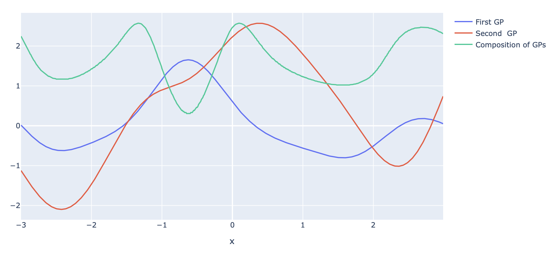
Figure 1: Composition of two Gaussian processes with SqExp covariance kernel $K(s,t)=e^{-(s-t)^{2}}$.

The recent seminal work by Finocchio and Schmidt–Hieber [20] on deepGPs shows that using a model selection prior to select active variables in the successive Gaussian processes, and conditioning individual GP sample paths to verify certain smoothness constraints, the induced posterior distributions contract nearly optimally and adaptively in quadratic loss for compositional structures in regression, for a variety of kernel choices. Focusing on compositions of constrained GPs (with bounded sample paths and derivatives), the paper [4] uses an adapted concentration function for deepGPs and derives near-optimal contraction rates in density estimation and classification. In [1], the authors investigate the use of deepGPs for a class of nonlinear inverse problems.

This work follows the footsteps of [20] and aims at answering the following two questions. The first concerns the possibility to obtain theory and optimality results for a deepGP construction as simple as possible that comes closer to current implementations of deepGPs in practice. The second concerns the possibility to allow for a high-dimensional ambient space as well as a smaller intrinsic dimension.

1. Can deepGP priors avoid an explicit model selection step?
   While the deepGP prior construction in [20] is completely natural and ‘canonical’ from the theoretical perspective, both the conditioning step (to match smoothness constraints) and the model selection prior (for which the posterior on submodels is often expensive to compute) make posterior sampling involved in view of practical implementation. One main objective here is to try to simplify the construction of the prior as much as possible while keeping optimality properties, and thereby come closer to the practically used deepGPs, for which lengthscale parameters are often kept free and then adjusted in an empirical Bayes [17] or hierarchical Bayes [41] fashion. In view of this last observation, we propose a prior with a ‘soft’ model selection based on a prior on lengthscales instead of the previous ‘hard’ model selection prior.

2. How do deepGPs scale with respect to ‘dimension’?
   Below we shall allow in some results the input space dimension $d$ to grow with $n$. Even though any method must then face a ‘curse of dimensionality’, if the effective ‘intrinsic’ dimension of the problem remains fixed or very slowly grows with $n$, it is conceivable that rates of convergence can still be obtained. While recent work on deep methods has shown that convergence rates only depending on intrinsic dimension(s) can be derived [42], most results are quite generous in the dependence on dimension of the constant factor in the rate. In particular, we are not aware of works allowing for input and ‘intrinsic’ dimensions to possibly grow with $n$ ([33] considers an example of Bayesian deep ReLU network with growing $d$ but fixed intrinsic dimension). We demonstrate below that our construction can adapt to the intrinsic dimension even for a high-dimensional ambient space (with $d$ sublinear in $n$). This requires a careful tracking of the dependence on dimension, in particular revisiting earlier results in the GP literature to make the dependence on $d$ precise.

The main contributions of the paper are as follows:

1. we introduce a new idea of freezing–of–paths for multi-bandwidth Gaussian processes. The benefit of random lengthscales of a stationary kernel for adaptation to smoothness has been established for a while [6, 34, 52, 54]. Such an adaptation to the regularity of the underlying truth is made possible by letting the lengthscales grow polynomially with $n$ in a suitable way with sufficient probability under the prior. In the present paper, we show that letting lengthscales appropriately vanish (instead of diverge) enables adaptation to structure (instead of smoothness) or in other words to perform variable selection, by ‘freezing’ irrelevant dimensions through the corresponding (tempered) posterior distributions. Intuitively, sample paths become almost constant in the directions with vanishing lengthscales, performing effectively a form of ‘soft’ model selection.

2. we show that the previous two effects of lengthscale parameters, namely adaptation to smoothness and to structure (by using respectively diverging and vanishing lengthscales), can be obtained using a single prior for lengthscales: the horseshoe distribution [8], that both puts a lot of mass near zero and at the tails, is shown to lead to optimal contraction rates with near-optimal scaling in terms of dimension. Our results also include exponential prior distributions on lengthscales as in earlier contributions on Gaussian processes (e.g. [54]), although dependence on dimension may not be optimal in ‘large $d$’ regimes.

3. we study high-dimensional variable selection for standard smoothness classes and for compositional structures; in particular we allow the input dimension to grow polynomially with $n$ and the number of actually relevant variables to grow slowly with $n$. A main technical contribution of the paper consists in deriving dimension-dependent analogues of the inequalities that are at the heart of GP regression theory with a squared-exponential kernel. Namely, we give precise dependence on ambient and intrinsic dimensions of the metric entropy of the unit ball of the RKHS of the covariance kernel, of the small ball probability of the GP and on quantities measuring approximation properties of this RKHS.

We note that the results are not only relevant for deep learning applications, but also already for shallow (standard) Gaussian processes, for which the freezing-of-paths effect described above is shown to lead to effective variable selection. Also, from the technical perspective, in order to leverage the smaller intrinsic dimensionality of the problem, a key new ingredient in the proofs consists in replacing the prior by a ‘low-dimensional’ oracle GP defined on the relevant coordinates. We also note that the results obtained in this paper are for tempered posterior distributions, where the tempering parameter can take any fixed value smaller than $1$; we refer to the discussion in Section 4 for more elements on this point and the currently open question of extending this to the standard posterior distribution (corresponding to a tempering parameter equal to $1$).

The paper is organised as follows: Section 2 introduces the statistical model and deep Gaussian process priors. We recall the main elements of a frequentist theoretical analysis of GP regression in Section 2.2. The main results are presented in Section 3: Theorem 2 deals with variable selection, possibly in high dimensions, for multibandwidth GPs. The case of adaptation to compositional structures via deep horseshoe GPs is considered in Theorems 3 and 4. A discussion follows in Section 4. Proofs are provided in Section 5. A key result underlying the proofs and bounding the GPs’ concentration function is presented in Section 6. Auxiliary lemmas and their proofs can be found in the appendix [12].

Notation. For two real numbers $a,b$, we let $a\wedge b=\min(a,b)$, $a\vee b=\max(a,b)$. We denote by $\phi$ the density of a standard normal random variable. The $\varepsilon$-covering number $N\left(\varepsilon,S,D\right)$ of a semimetric space $S$ equipped with a semimetric $D$ is the minimal number of balls of radius $\varepsilon$ needed to cover $S$. For a vector $A=\left(A_{1},\dots,A_{d}\right)$, denote

$$\bar{A}\coloneqq\underset{i=1,\dots,d}{\max}\ A_{i},\qquad|A|=\sum_{i}A_{i},$$

and $A_{I}=(A_{i})_{i\in I}$ for $I\subset[\![1,n]\!]$. For $f$ integrable on $\mathds{R}^{d}$, let $\hat{f}(t)=\int_{\mathds{R}^{d}}e^{-i\langle t,s\rangle}f(s)ds$ denote its Fourier transform, with ${\langle}\cdot,\cdot{\rangle}$ the euclidean inner product. In the following, $C,C_{1},c_{1},C_{2},c_{2},\dots$ denote absolute constants whose value may change from line to line.

2 The deep horseshoe GP prior

Consider a nonparametric regression model with random design, where one observes $(X,Y):=(X_{i},Y_{i})_{1\leq i\leq n}$, with $X_{1},\dots,X_{n}$ independent identically distributed design points sampled from a probability measure $\mu$ on $I^{d}$ for $I$ an interval of $\mathbb{R}$ chosen for simplicity to be $\left[-1,1\right]$ in the sequel and

$$Y_{i}=f_{0}(X_{i})+\varepsilon_{i},$$ (1)

for $f_{0}:I^{d}\to\mathbb{R}$ an unknown regression function and $\varepsilon_{i}$ independent $\mathcal{N}(0,\sigma_{0}^{2})$ errors, with $\sigma_{0}$ assumed known for simplicity. We consider estimation of $f_{0}$ with respect to the integrated quadratic loss

$$\left\lVert f_{0}-f\right\rVert_{L^{2}(\mu)}^{2}=\int(f_{0}-f)^{2}d\mu.$$

For a given regression function $f$, let $P_{f}$ denote the distribution of one observation $(X_{i},Y_{i})$ under model (1), which has density

$$p_{f}(x,y)=\left(2\pi\sigma_{0}^{2}\right)^{-1/2}e^{-(y-f(x))^{2}/(2\sigma_{0}^{2})}$$

with respect to $\mu\otimes\lambda$, for $\lambda$ the Lebesgue measure on $\mathbb{R}$.

For a real $\beta>0$, $\lfloor\beta\rfloor$ the largest integer strictly smaller than $\beta$ and $r$ an integer, let $\mathcal{C}^{\beta}[-1,1]^{r}$ denote the classical Hölder space equipped with the norm $\left\lVert\,\cdot\,\right\rVert_{\beta,\infty}$. It consists of functions $f:[-1,1]^{r}\to\mathbb{R}$ whose norm defined as

$$\left\lVert f\right\rVert_{\beta,\infty}=\max\left(\max_{|\boldsymbol{\alpha}|\leq\lfloor\beta\rfloor}\left\lVert\partial^{\boldsymbol{\alpha}}f\right\rVert_{\infty},\max_{\boldsymbol{\alpha}:|\boldsymbol{\alpha}|=\lfloor\beta\rfloor}\underset{\boldsymbol{x},\boldsymbol{y}\in[-1,1]^{d},\ \boldsymbol{x}\neq\boldsymbol{y}}{\sup}\frac{\left|\partial^{\boldsymbol{\alpha}}f(\boldsymbol{x})-\partial^{\boldsymbol{\alpha}}f(\boldsymbol{y})\right|}{\left|\boldsymbol{x}-\boldsymbol{y}\right|^{\beta-\lfloor\beta\rfloor}_{\infty}}\right)$$ (2)

is finite, with the multi-index notation $\boldsymbol{\alpha}=(\alpha_{1},\dots,\alpha_{d})\in\mathbb{N}^{d}$, $|\boldsymbol{\alpha}|\coloneqq|\boldsymbol{\alpha}|_{1}$ and $\partial^{\boldsymbol{\alpha}}=\partial^{\boldsymbol{\alpha}_{1}}\dots\partial^{\boldsymbol{\alpha}_{d}}$. We note that functions with finite Hölder norm are bounded, for any $\beta>0$.

2.1 Structural assumptions for multivariate regression

In order to assess the performance of machine learning methods, a popular benchmark is the regression setting (1) equipped with some ‘ structural’ assumptions. In the unconstrained case where only a smoothness condition is assumed on $f_{0}$, rates for $\beta$–Hölder smooth functions are typically of the form $n^{-\beta/(2\beta+d)}$, and so are prone to the curse of dimensionality (the rate becomes extremely slow for large $d$). A common approach is to assume that the multivariate regression function $f_{0}$ admits a certain unknown ‘structure’, of ‘effective dimension $d^{*}$’ possibly much smaller than $d$. For instance, in the simplest setting considered below, $f_{0}$ may only depend on a small but unknown number of coordinates. The goal is then to find algorithms that are able to achieve optimal risk bounds that adapt to the unknown underlying structure, and that therefore scale with $d^{*}$ instead of $d$.

A first basic setting: shallow variable selection. Let us first consider the simple setting where $f_{0}:\left[-1,1\right]^{d}=I^{d}\to\mathbb{R}$ only depends on $d^{*}$ variables, that is

$$f_{0}(x_{1},\dots,x_{d})=g(x_{i_{1}},\dots,x_{i_{d^{*}}}),$$ (3)

for some $g\in\mathcal{C^{\beta}}(I^{d^{*}})$ and $\beta>0$. The subset of indices $i_{1},\ldots,i_{d^{*}}$ is unknown to the statistician and the target convergence rate in quadratic loss is $n^{-\beta/(2\beta+d^{*})}$.

Define, for $K,\beta>0$ and $d^{*}\leq d$ two integers, and recalling that $I=[-1,1]$,

$$\mathcal{F}_{VS}(K,\beta,d,d^{*}) =\Big{\{}f_{0}:I^{d}\to\mathbb{R}\text{ such that }\eqref{vs}\text{ holds for some }g\in\mathcal{C}^{\beta}(I^{d^{*}}),$$ (4)

$$\quad\quad\left\lVert g\right\rVert_{\infty}\leq 1\text{ and }\|g\|_{\beta,\infty}\leq K\Big{\}}$$

As in recent works in deep learning and similar to [20], we assume that an upper-bound $M_{0}$ is known for the true function $f_{0}$ and without loss of generality we assume $M_{0}=1$.

Compositional structure. Following [42], suppose that $f$ can be written as a composition

$$f=h_{q}\circ\dots\circ h_{0},$$ (5)

with $h_{i}:\,I^{d_{i}}\to I^{d_{i+1}}$, for $(d_{i})$ a sequence of integers such that $d_{0}=d$ and $d_{q+1}=1$. Since $h_{i}$ takes values in $\mathbb{R}^{d_{i+1}}$, one may write $h_{i}=(h_{ij})$, where $h_{ij}$ for $j=1,\dots,d_{i+1}$ are its $1$–dimensional coordinate functions.

The compositional class $\mathcal{F}_{\text{deep}}(\lambda,\mathbb{\beta},K)$. Let us further assume that $h_{ij}$’s as above only depend on a subset $\mathcal{S}_{ij}$ of at most $t_{i}\leq d_{i}$ variables, and $h_{ij}$ restricted to the variables $\mathcal{S}_{ij}$ belongs to $\mathcal{C}^{\beta_{i}}(I^{t_{i}})$. For $\lambda=(q,d_{1},\dots,d_{q},t_{0},\dots,t_{q})$, $\mathbb{\beta}=(\beta_{0},\dots,\beta_{q})$ and $K>0$, let

$$\mathcal{F}_{deep}(\lambda,\mathbb{\beta},K)=\left\{h_{q}\circ\dots\circ h_{0}:\,I^{d}\to I,\ h_{i}:\,I^{d_{i}}\to I^{d_{i+1}},\ h_{ij}\in\mathcal{F}_{VS}(K,\beta_{i},d_{i},t_{i})\right\}.$$ (6)

Minimax optimal rate. The minimax rate of estimation in quadratic loss over this class

$$(r_{n}^{*})^{2}=\inf_{T}\sup_{f\in\mathcal{F}(\lambda,\mathbb{\beta},K)}E_{f}\|T-f\|_{2}^{2},$$

for $T$ ranging over the set of estimators of $f$, is, up to logarithmic factors,

$$r_{n}^{*}\asymp\underset{i=0,\dots,q}{\max}\ n^{-\frac{\beta_{i}\alpha_{i}}{2\beta_{i}\alpha_{i}+t_{i}}},\qquad\text{where }\alpha_{i}:=\prod_{l=i+1}^{q}(\beta_{l}\wedge 1),$$ (7)

under the mild condition $t_{i}\leq\min(d_{0},\ldots,d_{i-1})$, see [42].

2.2 Key ingredients

Posterior distributions and frequentist analysis. Given a prior distribution $\Pi$ on regression functions, the posterior mass $\Pi[B\,|\,X,Y]$ of a measurable set $B$ is given by Bayes’ formula: this is the next display for $\rho=1$. More generally, one may set, for any $\rho\in(0,1]$,

$$\Pi_{\rho}[B\,|\,X,Y]=\frac{\int_{B}\prod_{1\leq i\leq n}p_{f}(X_{i},Y_{i})^{\rho}d\Pi(f)}{\int\prod_{1\leq i\leq n}p_{f}(X_{i},Y_{i})^{\rho}d\Pi(f)}.$$

When $\rho=1$ this is the usual conditional probability that $f$ belongs to $B$ given the data. If $0<\rho<1$, this quantity is called ${\rho}$–posterior (or tempered posterior). Its use is very much widespread in machine learning, in particular in PAC–Bayesian settings [14, 58]. We use the tempered posterior in our main result, and discuss in more details the links with the case $\rho=1$ in Section 4.

Gaussian process ($\rho$–) posteriors: theory. For any centered Gaussian process $W$ on the Banach space of continuous functions on $I$ equipped with the $\left\lVert\,\cdot\,\right\rVert_{\infty}$ norm, the probability measure of any ball $\left\{f:\left\lVert f-g\right\rVert_{\infty}<\varepsilon\right\}$ is lower bounded by a quantity depending on the mass of the centered ball of radius $\varepsilon$ and on how well $g$ can be approximated by elements of the RKHS $(\mathbb{H},\left\lVert\,\cdot\,\right\rVert_{\mathbb{H}})$ of the covariance kernel of the process. More precisely, according to Proposition 11.19 of [22], for any $\varepsilon>0$,

$$P\left[\left\lVert W-g\right\rVert_{\infty}<\varepsilon\right] \geq e^{-\varphi_{g}(\varepsilon/2)},$$

$$\varphi_{g}(\varepsilon) =\underset{h\in\mathbb{H}:\ \left\lVert h-g\right\rVert_{\infty}\leq\varepsilon}{\inf}\frac{1}{2}\left\lVert h\right\rVert_{\mathbb{H}}^{2}-\log P\left[\left\lVert W\right\rVert_{\infty}<\varepsilon\right].$$ (8)

The function $\varphi_{g}$ in (2.2) is called the concentration function of the Gaussian process $W$ and plays a key role in the study of contraction rates for GPs [53]. It is the sum of two terms: the first term with the infimum is the approximation term whereas the second term is called the small ball term (the probability within the log is the small ball probability of the process $W$).

In nonparametric regression with fixed design, [54] proved that posterior contraction rates that are adaptive to the unknown smoothness of the regression function are achievable for stationary Gaussian process priors, with a dilatation parameter of the sample paths distributed as a Gamma variable. As a particular case, consider the squared exponential process SqExp defined as the zero-mean Gaussian process with covariance kernel $K(s,t)=\exp(-\left\lVert t-s\right\rVert^{2})$ (and $\left\lVert\,\cdot\,\right\rVert$ the euclidean norm) on $[-1,1]^{d}$. Next, for $k,\theta>0$, one sets

$$A^{d} \sim\text{Gamma}\left(k,\theta\right)$$

$$f\ \big{|}\ A \sim\left\{W_{At}:\ t\in[-1,1]^{d}\right\}.$$

This construction induces a prior on the Banach space of continuous functions for which the posterior concentrates in the empirical $L_{2}-$norm at rate $\varepsilon_{n}\asymp n^{-\beta/(2\beta+d)}$ (up to a log factor) whenever $f_{0}$ has $\beta$-Hölder regularity, $\beta>0$.

Although this rate coincides with the minimax estimation rate over a ball in $\mathcal{C^{\beta}}[-1,1]^{d}$, it becomes very slow for large $d$. However, if the fixed design is located on a $d^{*}$-dimensional Riemannian manifold, $d^{*}<d$, of the ambient space $[-1,1]^{d}$, we expect the faster rate $n^{-\beta/(2\beta+d^{*})}$ to be attainable. The work [56] achieves it with a dilated Gaussian process as well, the dilatation factor $A$ being distributed as $A^{d^{*}}\sim\text{Gamma}\left(k,\theta\right)$. One may note that this approach requires an estimate of $d^{*}$ to be applied and that posterior contraction rates are obtained for local distances on the manifold (such as the empirical $L_{2}$-norm) only, but not on the ambient space.

When the regression function $f_{0}$ depends on a small number of variables $d^{*}$ only, a special case of the add-GP prior from [57] gives optimal posterior contraction rates $n^{-\beta/(2\beta+d^{*})}$ without the need to estimate $d^{*}$. This is achieved by the introduction of an additional layer in the prior, drawing via Bernoulli random variables in which direction the Gaussian sample paths have to be dilated (the sample paths being constant in the other directions). From a practical point-of-view, this ‘hard’ selection of variables adds a combinatorial complexity to posterior sampling.

Below, we introduce the Horseshoe Gaussian process prior to answer the question of variable selection and posterior contraction rates for the most natural global $L^{2}$ loss (in contrast to a loss e.g. restricted only on active directions) via a soft selection of dilated variables.

2.3 Deep Horseshoe Gaussian Process prior

We introduce a Gaussian process prior with independent inverse–lengthscales distributed following a half-horseshoe distribution. This distribution possesses two interesting properties for our goals. Its density has a pole at $0$, which allows to ‘freeze’ irrelevant dimensions, drawing small inverse lengthscales with high probability. It also has heavy tails, so that it performs an adequate scaling on the ambient dimensions with sufficiently large probability.

The single-layer case. In the following, we use the real map

$$\Psi\colon\ x\mapsto\left(x\wedge 1\right)\ \vee\ (-1).$$

For $\pi$ a density function on $\mathbb{R}_{+}$, consider the following prior $\Pi$ on regression functions $f$

$$A_{j} \overset{\text{i.i.d.}}{\sim}\pi$$ (9)

$$f\ |\ (A_{1},\dots,A_{d}) \sim\Psi(W^{A}),$$

where

$$W^{A}=\left\{W_{(A_{1}s_{1},\dots,A_{d}s_{d})}:\ s=(s_{1},\dots,s_{d})\in[-1,1]^{d}\right\},$$

for $W$ the squared exponential process SqExp. For a given value of $A$, we call $W^{A}$ a multibandwidth Gaussian process.

Although the theory below can be applied to arbitrary scaling distributions $\pi$, we consider two main examples in the sequel: an exponential and a horseshoe distribution. Let us define $\pi_{\tau}$, $\tau>0$, as the (half-) horseshoe density (introduced in [8]) i.e. the density of a random variable $X_{\tau}$ distributed as

$$\xi \sim C^{+}(0,1)$$

$$X_{\tau}\ |\ \xi\ \sim\mathcal{N}^{+}(0,\tau^{2}\xi^{2}),$$

with $C^{+}(0,1)$ a standard half-Cauchy distribution and $\mathcal{N}^{+}(\mu,\sigma^{2})$ the half-normal distribution of $|X|$, $X\sim\mathcal{N}(\mu,\sigma^{2})$. We refer to [49] for posterior contraction results in the case of estimation of sparse vectors, with priors based on $\pi_{\tau}$ and discussions on the influence of $\tau$.

When $\pi=\pi_{\tau}$ the horseshoe density on $\mathds{R}_{+}$ in (9), we call the above hierarchical prior the Horseshoe Gaussian Process prior and denote it $\textsf{HGP}(\tau)$.

The multi-layer case. In order to perform inference in more complex models, we introduce a deepGP-type prior, mixing ideas from [20] and the just introduced prior (9).

We first place discrete priors $\Pi_{q}$ on the number of layers $q$ and $\Pi_{d}[d_{1},\dots,d_{q}|q]$ on the successive ambient dimensions in the composition (5). We assume that $\Pi_{q}[q]>0$ and $\Pi_{d}[d_{1},\dots,d_{q}|q]>0$ for any integers $q\geq 0$ and $d_{i}\geq 1$.

Given $q,d_{1},\ldots,d_{q}$, we define a random regression function $f=W_{q}\circ\dots\circ W_{0}$ where, for $i=0,\dots,q$, the map $W_{i}\colon I^{d_{i}}\to\mathbb{R}^{d_{i+1}}$ is a multivariate Gaussian process indexed by $I^{d_{i}}$ and $\Psi$ is applied element-wise. We assume that for $j=1,\dots,d_{i+1}$, the coordinates $(W_{i})_{j}$ are independently (accross $i$ and $j$) and identically (across $j$) distributed as a prior of the form (9). Constraining the sample paths between $-1$ and $1$ ensures that the composition is well-defined.

The Deep Horseshoe Gaussian Process Deep–HGP is a special case of this construction where the prior on lengthscales is a horseshoe prior: it is defined as the hierarchical prior

$$\begin{split}q&\sim\Pi_{q}\\ d_{1},\dots,d_{q}\ |\ q&\sim\Pi_{d}[\cdot|q]\\ g_{ij}\ |\ (q,d_{1},\dots,d_{q})&\overset{\text{ind.}}{\sim}\textsf{HGP}(\tau_{i})\\ f\ |\ (q,d_{1},\dots,d_{q},g_{ij})&=g_{q}\circ\dots\circ g_{0}.\end{split}$$ (10)

for $\tau_{i}>0$, $i=0,\ldots,q$. In the above, $g_{i}=(g_{ij})_{j}$ with $g_{ij}:I^{d_{i}}\to I$, $1\leq j\leq d_{i+1}$.

Some comments are in order. Here for full flexibility we draw first a prior on the number of compositions $q$ and ‘inner’ dimension parameters $d_{1},\ldots,d_{q}$: at the $j$–th level of the composition, there are $d_{j+1}$ coordinate functions $(g_{ij})$ distributed as the HGP process, each of these functions depending on $d_{j}$ parameters (and setting $d_{q+1}=1$ the output dimension). Note that on each layer $j$, all $d_{j}$ variables are present simultaneously as input to each Gaussian process component, although the scalings (distributed as horseshoe random variables) calibrate the ‘strength’ (or ‘importance’) of these variables.

3 Main results: deep simultaneous adaptation to structure and smoothness

To gain intuition on our proposed procedure, we now build up progressively the results, starting from a standard smoothness condition in regression (no composition) where the regression function depends on an effective number of coordinates possibly smaller than the input dimension $d$. Section 3.1 presents a simple oracle result while Section 3.2 considers more precise results allowing for adaptation and growing dimension. The ‘deep’ case of compositional structures is considered in Section 3.3. Recall that $\sigma_{0}^{2}$ is the variance of the noise in (1) and set

$$\xi:=2\sigma_{0}^{2}/\sqrt{1+4\sigma_{0}^{2}}.$$ (11)

3.1 “Freezing of paths" for variable selection: a new effect of scaling for Gaussian processes

The first result assumes that the true regression function depends on a number $d^{*}$ of coordinates only, and that for now the indices of the active variables are known.

Theorem 1 (freezing of paths).

Let $d\geq 2$ be a fixed integer and for $K\geq 1,\beta>0$, set $\mathcal{F}(K):=\mathcal{F}_{VS}(K,\beta,d,d^{*})$. Fix $\rho\in(0,1)$, let $f_{0}\in\mathcal{F}(K)$ and suppose

$$f_{0}(x_{1},\ldots,x_{d})=g_{0}(x_{i_{1}},\ldots,x_{i_{d^{*}}}),$$

with $S_{0}:=\{i_{1},\ldots,i_{d^{*}}\}\subset\{1,\ldots,n\}$ and some $1\leq d^{*}\leq d$. Let $\Pi$ be a multibandwidth prior

$$f(x)\sim\Psi(W_{(a_{1}x_{1},\ldots,a_{d}x_{d})})$$

with $W$ a $d$–dimensional SqExp Gaussian process with deterministic scaling parameters

$$a_{i}=\begin{cases}n^{\frac{1}{2\beta+d^{*}}},&\quad\text{if }i\in S_{0}\\ 1/\sqrt{n},&\quad\text{if }i\notin S_{0}\end{cases}.$$ (12)

Then, there exists $M>0$ such that the $\rho$–posterior $\Pi_{\rho}[\cdot\,|\,X,Y]$ verifies

$$\sup_{f_{0}\in\mathcal{F}(K)}E_{f_{0}}\Pi_{\rho}\left[f:\ \left\lVert f-f_{0}\right\rVert_{L^{2}(\mu)}\geq M\log^{1+d^{*}}(n)n^{-\frac{\beta}{2\beta+d^{*}}}\,|\,X,Y\right]\to 0.$$

Theorem 1 shows that by taking GP lengthscale parameters that are very small, of order $1/\sqrt{n}$, for the coordinates $j$ such that $f_{0}$ in fact does not depend on $x_{j}$, and taking lengthscales equal to the ‘standard nonparametric cut-off’ $n^{1/(2\beta+d^{*})}$ (for estimating $\beta$–smooth functions in dimension $d^{*}$) on the other coordinates, leads to an optimal minimax contraction rate $n^{-\beta/(2\beta+d^{*})}$ for the integrated squared loss up to a logarithmic factor for the $\rho$–posterior distribution (the power in the log factor is improved in the next result). Inspection of the proof shows that for $i\notin S_{0}$, one may take $a_{i}$ to be any value smaller than $C/\sqrt{n}$ for some fixed $C>0$.

The intuition behind the result is that taking a small lengthscale for coordinate $i$ ‘freezes’ the GP path along this coordinate, making it almost constant in that coordinate, which corresponds to the limiting case $a_{i}=0$. Note that Theorem 1 is an ‘oracle’ result in that it assumes both $\beta$ and $d^{*}$ (and even the indices $i_{j}$) to be known. Adaptive versions are considered below. While the result is somewhat expected if one sets $a_{i}=0$ for $i\notin S_{0}$ (this would correspond to a ‘hard’ variable selection), the fact that the rate remains optimal for small but non-zero values of $a_{i}$ suggests that there may be room for a ‘soft’ variable selection procedure that would allow for small $a_{i}$ in a data-driven way: this is the purpose of our next Theorem.

3.2 Single layer setting: horseshoe GP

The next statement is our main result on variable selection for (non-deep) Gaussian processes. It is a non-asymptotic result that allows for dimensions varying with $n$. It is stated for an arbitrary prior $\pi$ on lengthscales. We then particularise it over the next paragraphs by stating simpler asymptotic versions and giving examples of lengthscale priors that satisfy the conditions. We consider both the fixed dimensional case and the case where both $d^{*}$ and $d$ vary with $n$.

Theorem 2 (Variable selection).

Let $1\leq d^{*}\leq d$ be two integers and for $K\geq 1,\beta>0$, set $\mathcal{F}(K):=\mathcal{F}_{VS}(K,\beta,d,d^{*})$. Let $\xi$ be as in (11) and fix $0<\rho<1$. Let $\Pi$ be a multibandwidth prior (9) with density $\pi$ on scaling parameters that satisfies

$$\left(\int_{0}^{\frac{\xi}{8d\sqrt{\rho n}}}\pi(a)da\right)^{d-d^{*}}\left(\int_{a^{*}}^{2a^{*}}\pi(a)da\right)^{d^{*}}\geq 2\exp(-n\rho\varepsilon_{n}^{2}/2),$$ (13)

where $a^{*}=a_{n}^{*}$ and $\varepsilon_{n}$ verify $a^{*}\geq 1$, that $1/\sqrt{n}\leq\varepsilon_{n}\leq 1$, and

$$64\xi^{-2}\geq\varepsilon_{n}^{2}\geq\{B_{1}{a^{*}}^{-2\beta}\}\vee\{B_{2}{a^{*}}^{d^{*}}\log^{1+d^{*}}(n)/n\},$$ (14)

where $B_{1}=c_{1}K^{2}c_{2}^{d^{*}}$ and $B_{2}=K^{2}(c_{3}d^{*c_{4}})^{d^{*}}$, with $c_{1},\ldots,c_{4}\geq 1$ constants depending only on $\beta$, $\xi$ and $\rho$. Then, there exists $M=M(\rho,\xi)>0$ such that, for $n\geq 3$,

$$\sup_{f_{0}\in\mathcal{F}(K)}E_{f_{0}}\Pi_{\rho}[f:\ \left\lVert f-f_{0}\right\rVert_{L^{2}(\mu)}\geq M\varepsilon_{n}\,|\,X,Y]\leq\frac{1}{n\varepsilon_{n}^{2}}+e^{-\rho n\varepsilon_{n}^{2}}.$$

Theorem 2 gives a contraction of the $\rho$–posterior distribution at rate $\varepsilon_{n}$ around the true $f_{0}$, provided $n\varepsilon_{n}^{2}$ is suitably large. A more explicit expression of $\varepsilon_{n}$ is given in the next Corollary.

Corollary 1 (Optimal $a^{*}$ and posterior rate).

Optimising $a^{*}$ in (14), leads to setting

$$(a^{*})^{2\beta+d^{*}}=(B_{1}n)/(B_{2}\log^{1+d^{*}}(n))\vee 1.$$ (15)

Condition (14) then becomes, for $a^{*}$ as in (15),

$$64\xi^{-2}\geq\varepsilon_{n}^{2} \geq\left[B_{3}(\log{n})^{\frac{2\beta(1+d^{*})}{2\beta+d^{*}}}n^{-\frac{2\beta}{2\beta+d^{*}}}\right]\vee\left[B_{2}\log^{1+d^{*}}(n)/n\right],$$ (16)

where $B_{3}=K^{2}c_{5}^{d^{*}}d^{*d^{*}\frac{c_{6}}{2\beta+d^{*}}}$, recalling $B_{2}=K^{2}(c_{3}d^{*c_{4}})^{d^{*}}$, and $c_{3},\ldots,c_{6}\geq 1$ are constants only depending on $\beta,\xi,\rho$. If additionally (13) holds (conditions for this are given below), then the $\rho$–posterior rate can be taken as the right-hand side of (16).

In the asymptotic regime $n\to\infty$, for $\varepsilon_{n}$ taken equal to the right hand-side of (16), it follows that $\varepsilon_{n}\to 0$ and $n\varepsilon_{n}^{2}\to\infty$, so that provided (13) holds, the posterior mass in the last display of Theorem 2 goes to $0$, and the posterior contracts to $f_{0}$ at rate $\varepsilon_{n}$ asymptotically. For reasonable (i.e. fixed or growing slowly with $n$) values of $d^{*}$, the first term in (16) dominates and, again under (13), the resulting rate $\varepsilon_{n}$ goes to $0$ with $n$. Next we investigate a few examples of priors for which (13) holds with a resulting $\varepsilon_{n}$ given by (16).

The proof of Theorem 2 is based on considering an oracle process defined on the $d^{*}$ relevant dimensions. The rates can then carry over to the full prior thanks to Condition (13), which ensures that the lengthscale prior $\pi$ tunes down irrelevant dimensions, so that the difference between the processes is small with high probability. These deviations are controlled via new dimension–dependent estimates of characteristics of the squared-exponential Gaussian process (via its RKHS), see Theorem 5 and Lemmas 2–4, coupled with concentration of measures tools. This theorem is a main theoretical novelty of the paper: a lengthscale prior which puts large mass on small values allows to ‘freeze’ irrelevant directions, so that the overall prior behaves like a smaller-dimensional one.

Fixed dimensions. Let us now examine the case where the dimensions $d,d^{*}$ are fixed, independent of $n$. We derive conditions on two natural priors: an exponential prior, as used e.g. in [53] for adaptation to smoothness, and a horseshoe prior.

Example 1 (Exponential prior with fixed scaling $\lambda$).

Consider $\pi(a)=\lambda e^{-\lambda a}1\!{\rm l}_{a>0}$ an exponential prior of parameter $\lambda>0$. A simple calculation, see Lemma 16, shows that (13) is verified if

$$n\varepsilon_{n}^{2}\geq(2/\rho)\left[d\log\left(\frac{16d\sqrt{\rho n}}{\xi\lambda}\right)+2\lambda d^{*}a^{*}+\log 2\right],$$ (17)

as long as $\lambda\in[1/a^{*},8d\sqrt{\rho n}/\xi]$. As a particular case, for fixed $d,d^{*},K,\lambda$, and $a^{*}$ as in (15), this condition is automatically satisfied for large enough $n$ if (16) holds.

Example 2 (Horseshoe prior with fixed parameter $\tau$).

Consider $\pi=\pi_{\tau}$ a horseshoe prior of parameter $\tau>0$. Then (13) is verified if, setting $e_{0}=2/(2\pi)^{3/2}$,

$$n\varepsilon_{n}^{2}\geq(2/\rho)\left[d\log\left(\frac{8d\sqrt{\rho n}}{\xi e_{0}\tau}\right)+d^{*}\log(10a^{*}/\tau)+\log 2\right],$$ (18)

as long as $\tau\in[\xi/(8d\sqrt{\rho n}),a^{*}]$, see Lemma 17. In particular, for fixed $d,d^{*},K,\tau$, and $a^{*}$ as in (15), this condition is automatically satisfied for large enough $n$ if (16) holds.

To obtain (18), one simply uses that the horseshoe density is bounded from below by a constant on the integration interval; this is sensible for a fixed $\tau$ but can be significantly improved for small $\tau$, as seen below.

Corollary 2 (Fixed dimensions).

In the setting of Theorem 2, suppose the input dimension $d$ is fixed (independent of $n$). Let $\pi$ be either the exponential prior or the horseshoe prior with fixed (independent of $n$) respective parameters $\lambda$ and $\tau$. Then for large enough $M>0$ (depending on $\beta,d^{*}$ only), as $n\to\infty$,

$$\sup_{f_{0}\in\mathcal{F}(K)}E_{f_{0}}\Pi_{\rho}[f:\ \left\lVert f-f_{0}\right\rVert_{L^{2}(\mu)}\geq M\varepsilon_{n}\,|\,X,Y]\to 0,$$

where $\varepsilon_{n}$ is given by $\varepsilon_{n}=(\log{n})^{\frac{2\beta(1+d^{*})}{2\beta+d^{*}}}n^{-\frac{2\beta}{2\beta+d^{*}}}$. In particular, the posterior distribution achieves the minimax convergence rate up to a logarithmic factor.

An important consequence of Corollary 2 is that it is possible to derive a (near-)optimal rate adapting to the unknown number $d^{*}$ and coordinates of the active variables with continuous priors, that is, even without setting the scaling exactly to zero on certain coordinates (i.e. without performing a ‘hard model selection’). Even more surprisingly at first, such ‘soft model selection’ is possible (at least with tempered posteriors) using a prior not putting a particularly large amount of mass near $0$, such as an exponential prior. In particular, simple priors on scalings such as exponentials or gamma distributions considered in [53] have prior mass permitting for ‘enough’ variable selection in order for their (tempered)–posterior distribution to contract at near optimal rate, without using oracle knowledge of which coordinates are active or not.

At this point it may seem as if variable selection can be achieved at no cost with just simple random scalings on coordinates. This is not (completely) so, the reason being that the dependence on the input dimension $d$ in the convergence rate that arises from e.g. putting exponential priors on scalings is far from optimal. This can be seen from (17), or similarly (18) for $\pi_{\tau}$ with fixed $\tau$, as follows. Recall that (17)–(18) are non-asymptotic conditions, so one may let $d,d^{*}$ depend on $n$. Suppose for instance $d=n^{\delta}$ for some $\delta>0$ and $d^{*}$ is fixed, say $d^{*}=1$ to fix ideas. Then (17) cannot hold with $\varepsilon_{n}$ the lower bound in (16): indeed, the latter is up to a log-factor of order $n^{1/(2\beta+1)}$, so is a $o(n^{\delta})$ as soon as $\delta>1/(2\beta+1)$, which shows that in this setting the rate is suboptimal for large enough $\beta$’s.

The previous comments naturally make one wonder if variable selection is still feasible with a better dependence on dimensions with continuous scaling. The next section investigates this, in a setting where $d$ can go to $\infty$ with $n$.

High-dimensional variable selection. Let us now study the problem of variable selection if $d$ is possibly allowed to depend on $n$. In the high-variable selection problem as in the first setting of Section 2.1, the work [57] derives up to constants the minimax rate of estimation for the squared $\left\lVert\,\cdot\,\right\rVert_{L^{2}(\mu)}$ loss which is up to a constant factor depending on $K$, $\beta$ and $d^{*}$,

$$(\epsilon_{n}^{*})^{2}\asymp n^{-\frac{2\beta}{2\beta+d^{*}}}+\frac{d^{*}}{n}\log(d/d^{*}).$$

The first term corresponds to the rate of estimation of a low-dimensional function $g\in\mathcal{C}^{\beta}[-1,1]^{d^{*}}$ and the second is the rate for the variable selection problem. Under Condition (19) below, the first term dominates. Note however that, as the dependence of the constants in $d^{*}$ is not explicit in the last display, this result allows for $d\to\infty$ and a fixed $d^{*}$ but not both $d^{*},d$ going to infinity.

Let us consider the high-dimensional variable selection setting where $d$ can go to infinity; we also allow the effective dimension $d^{*}$ to slowly grow with $n$: more precisely for some $\delta<1/2$ and $C_{1},C_{2}>0$ suppose

$$1\leq d^{*}\leq(\log{n})^{1/2-\delta},\qquad 1\leq d^{*}\leq d\leq C_{1}n^{C_{2}}.$$ (19)

One may hope to obtain a convergence rate that depends on the effective dimension $d^{*}$ only, not on $d$. In Appendix E [12], Corollary 4, we derive a lower bound result that shows that under mild conditions on the design distribution, and if the radius of the considered Hölder ball is not too large, the minimax rate for the integrated quadratic risk is bounded below by $C_{2}D_{2}^{d^{*}}n^{-2\beta/(2\beta+d^{*})}$, for constants $C_{2},D_{2}$ independent of $d^{*}$. We show below that this rate can be achieved by a well-chosen horseshoe GP in the regime (19), up to a slowly-varying term $D_{3}^{d^{*}}$. To do so, one first determines a horseshoe scaling parameter $\tau$ for which condition (13) holds, and then we state the high-dimensional variable selection result as Corollary 3 (more details on optimality can be found below in Section E Corollary 4).

Example 3 (Horseshoe prior with vanishing parameter $\tau$).

Consider $\pi=\pi_{\tau}$ a horseshoe prior of parameter $\tau>0$. Then (13) is verified for large enough $n$ if

$$10a^{*}e^{-n\rho\varepsilon_{n}^{2}/2d^{*}}\leq\tau\leq\frac{\xi}{d^{2}}\frac{1}{\sqrt{\rho n}}$$ (20)

For $a^{*},\varepsilon_{n}$ as in (15)–(16), the last display holds for large enough $n$ and fixed $K$ (or more generally $K\leq C^{d^{*}}$ for some $C>1$) if one sets for some $\delta>0$

$$\tau=\tau^{*}:=(n^{1+\delta}d^{4})^{-1/2}.$$

For a proof of both claims, see Lemma 18.

Corollary 3 (High-dimensional horseshoe GP).

In the setting of Theorem 2, suppose $d^{*},d$ verify Condition (19). Let $\Pi$ be the multibandwidth prior (9) with horseshoe scaling density $\pi_{\tau^{*}}$ and $\tau^{*}=(n^{1+\delta}d^{4})^{-1/2}$, $\delta>0$. Then, for $K\geq 1$, there exists $M=M(\xi,\rho)>0$ such that

$$\sup_{f_{0}\in\mathcal{F}(K)}E_{f_{0}}\Pi_{\rho}[f:\ \left\lVert f-f_{0}\right\rVert_{L^{2}(\mu)}\geq M\varepsilon_{n}\,|\,X,Y]\to 0,$$

as $n\to\infty$ where, for some constant $C$ that depends on $\beta,\xi,\rho$ only,

$$\varepsilon_{n}^{2}=K^{2}C^{d^{*}}(\log{n})^{\frac{2\beta(1+d^{*})}{2\beta+d^{*}}}n^{-\frac{2\beta}{2\beta+d^{*}}}.$$

In particular, for $K^{2}\leq C^{d^{*}}$, the rate $\varepsilon_{n}^{2}$ is of order $n^{-2\beta/(2\beta+d^{*})}$, up to a smaller order term at most of order $C^{2d^{*}}(\log{n})^{\frac{2\beta(1+d^{*})}{2\beta+d^{*}}}$.

The rate $\varepsilon_{n}^{2}$ obtained in Corollary 3 is optimal in the minimax sense up to the smaller order term $K^{2}C^{d^{*}}$ (up to a log factor). As mentioned above, as long as $K$ does not grow faster than $C_{4}^{d^{*}}$ this is a slower order term compared to the main term $n^{-2\beta/(2\beta+d^{*})}$ (in regime (19)) in the minimax lower bound from Corollary 4: in this case the rate is minimax optimal up to a slower order term $C_{5}^{d^{*}}$. We also note that a growth in $C^{d^{*}}$ for the radius $K$ of the Hölder ball is typical for functions in Hölder spaces of dimension $d^{*}$, see Appendix D [12], where this is checked for functions of product form.

The idea behind Corollary 3 is that for small values of the parameter $\tau$, the horseshoe distribution becomes very ‘sparse’ in the sense that most nonzero values are very close to $0$: this is reminiscent of the high-dimensional statistics literature for sparse models, see e.g. [50, 48], where near-optimal posterior rates for horseshoe posteriors are derived in sparse settings. We now turn to a deep learning setting, where the Gaussian process is allowed to have several compositional layers.

3.3 Multilayer setting: Deep Horseshoe GP

We go back for now to the fixed dimensional case, but we consider the additional problem of adaptation to an unknown compositional structure. The following result shows that, assuming the regression function can be expressed as a composition (5), such adaptation can be achieved with a prior mimicking this structure and organizing Gaussian processes in layers. In particular, in the Deep–HGP prior, the distribution on the scalings of the individual Gaussian processes allows for adaptation to the regularity as we have seen above, but also adaptation to a sparse network of compositions.

Theorem 3.

Let $\lambda=(q,d_{1},\dots,d_{q},t_{0},\dots,t_{q})$, $\mathbb{\beta}=(\beta_{0},\dots,\beta_{q})$, $d\geq 1$, $K\geq 1$ and suppose $f_{0}\in\mathcal{F}_{\text{deep}}(\lambda,\mathbb{\beta},K)$. Let $\Pi$ be the Deep–HGP prior (10) with fixed parameters $\tau_{i}>0$. Then, for any $0<\rho<1$, $\Pi_{\rho}[\cdot\,|\,X,Y]$ contracts to $f_{0}$ at the rate

$$\varepsilon_{n}=\max_{i=0,\dots,q}(\log{n})^{\frac{\alpha_{i}\beta_{i}(1+t_{i})}{2\alpha_{i}\beta_{i}+t_{i}}}n^{-\frac{\alpha_{i}\beta_{i}}{2\alpha_{i}\beta_{i}+t_{i}}}$$

in $\left\lVert\,\cdot\,\right\rVert_{L^{2}(\mu)}$ distance, where $\alpha_{i}=\prod_{l=i+1}^{q}(\beta_{l}\wedge 1)$: for any $M_{n}\to\infty$

$$E_{f_{0}}\Pi_{\rho}[f:\ \left\lVert f-f_{0}\right\rVert_{L^{2}(\mu)}\geq M_{n}r_{n}\,|\,X,Y]\to 0.$$

Theorem 3 shows that the fractional posterior attains the minimax rate of convergence of contraction (7) over the class $\mathcal{F}_{\text{deep}}(\lambda,\beta,K)$ up to the logarithmic factor $\log^{\gamma}n$, $\gamma=\max_{i=0,\dots,q}\ 2\alpha_{i}\beta_{i}(1+t_{i})/(2\alpha_{i}\beta_{i}+t_{i})$. For simplicity, we only considered the situation where inverse-bandwidths are distributed as horseshoe random variables. As above in the fixed $d$ setting with GPs, one can derive similar results for exponential priors on scalings. However, given the benefits of the horseshoe prior in high-dimensional settings (see also below), we focus on this choice.

Theorem 3 can be compared to Theorem 2 of [20], providing rates for a deepGP construction over a compositional functional class. The present result on the Deep–HGP prior now shows that adaptation to the structure can be achieved with $\rho$–posteriors without imposing a hyperprior on all the parameters describing the structure. It is sufficient to specify a prior on the depth and width of the composition. As in our results of Section 3.2 on (single-layer) GPs, instead of imposing a ‘hard’ selection of relevant variables on each layer, a continuous distribution on the lengthscales, with sufficient mass on small values, is enough for simultaneous adaptation to smoothness and sparse compositional structure.

In view of Corollary 3, one naturally wonders if the Deep–HGP prior is able to perform adaptation to the structure and the regularity in a high-dimensional framework as well. More precisely, suppose $f_{0}:\left[-1,1\right]^{d}\to\mathbb{R}$ belongs to $\mathcal{F}_{\text{deep}}(\lambda,\mathbb{\beta},K)$ with $d=d_{0}$ and $t_{0}$ possibly depending on $n$. As in (19), we suppose $t_{0},d_{0}$ verify, for some $\delta<1/2$ and $C_{1},C_{2}>0$,

$$1\leq t_{0}\leq(\log{n})^{1/2-\delta},\qquad 1\leq t_{0}\leq d_{0}=d\leq C_{1}n^{C_{2}}.$$ (21)

The next result shows that letting the horseshoe scale parameter $\tau_{0}$ of the first layer in the composition vanish in the Deep–HGP prior, while keeping the other scale parameters $\tau_{i},i=1,\ldots q$ across the other layes, constant, is enough to still obtain a near-minimax rate of contraction for the fractional posterior. Choosing $\tau_{0}$ appropriately small (although independent of the true unknown $t_{0}$) allows one obtain sparsity on the first layer, mitigating the effect of the growing input dimension $d$.

Theorem 4.

Under the same assumptions as in Theorem 3, now suppose $t_{0}$ and $d_{0}$ satisfy Condition (21), and that $d_{1},\ldots,d_{q}$ are fixed, non $n$–dependent integers. Let $\Pi$ be the Deep–HGP prior with $\tau_{0}=d^{-2}n^{-1}$ and $\tau_{i}>0,i=1,\ldots,q$ be fixed. For any $0<\rho<1$, there exists $c_{1},c_{2}$ depending on $\beta_{0}$ and $\rho$ such that the $\rho$–posterior contracts to $f_{0}$ at the rate

$$\varepsilon_{n}^{2}=\left[c_{1}K^{2}c_{2}^{t_{0}}(\log{n})^{\frac{2\beta_{0}\alpha_{0}(1+t_{0})}{2\beta_{0}\alpha_{0}+t_{0}}}n^{-\frac{2\beta_{0}\alpha_{0}}{2\beta_{0}\alpha_{0}+t_{0}}}\right]\vee\max_{i=1,\dots,q}(\log{n})^{\frac{2\alpha_{i}\beta_{i}(1+t_{i})}{2\alpha_{i}\beta_{i}+t_{i}}}n^{-\frac{2\alpha_{i}\beta_{i}}{2\alpha_{i}\beta_{i}+t_{i}}}$$

in $\left\lVert\,\cdot\,\right\rVert_{L^{2}(\mu)}$ distance, that is, for any $M_{n}\to\infty$,

$$E_{f_{0}}\Pi_{\rho}[f:\ \left\lVert f-f_{0}\right\rVert_{L^{2}(\mu)}\geq M_{n}\varepsilon_{n}\,|\,X,Y]\to 0.$$

To the best of our knowledge, Theorem 4 is the first result on deep methods in high-dimensional regression where both the input dimension $d_{0}=d_{0}(n)$ and first effective dimension $t_{0}=t_{0}(n)$ are allowed to grow with $n$. It combines both the ability of the horseshoe prior to select relevant dimensions in the input space and its ability to perform model selection in presence of a compositional parameter. It is particularly interesting given that these methods are most often applied to high-dimensional problems.

Compared to the condition on $\tau$ in Corollary 3, the preceding result requires a smaller $\tau_{0}$. In the present setting, given the flexibility of the sample paths from deep Gaussian processes, it is necessary to ’stabilize’ each GP to avoid ’wild’ behavior. From a technical point of view, it translates into more restrictive prior mass conditions for these GPs and the need for more efficient variable selection. This is achieved with a horseshoe prior that is more peaked near $0$, given the choice of the smaller parameter.

Remark 1.

In Theorem 4, we let the dimensions indexed by $i=0$ on the first layer of the composition to possibly grow with $n$. Extending this result to a situation where $d_{i},i>0$ can also grow with $n$ is not straightforward. Indeed, inspection of the proof of Theorems 3 and 4 shows that the rate involves a multiplicative factor $\sum_{i=1}^{q+1}d_{i}$ whose dependence on the inner dimensions of the composition is linear and thus prevents polynomially growing $d_{i}$’s. As this factor does not involve $d_{0}$, it still allows for $t_{0},d_{0}$ as in (21).

4 Discussion and open questions

In this work, we provide theoretical guarantees for the convergence of fractional posterior distributions using deep Gaussian process priors. One key insight is in the role played by lengthscale parameters: not only do these enable adaptation to smoothness, but they can also at the same time perform variable selection by ‘freezing’ the Gaussian process paths in suitable directions, a point relevant also for standard (non-deep) Gaussian processes; this has not been recognised so far in the literature to the best of our knowledge. The fact that adaptation to smoothness and structure can be performed simultaneously is particularly appealing computationally in that there is no need to include a model selection part in the building of the prior (if that was the case, posterior sampling would require to have access to the posterior distribution over models, which is often costly to implement). The obtained deepGP prior is then simple enough so that it corresponds to recently proposed algorithms, see below for more on this. One possible (at least formal) limitation to our results is the fact that the results are valid for any fractional posterior ($\rho<1$) but that they do not apply to the standard posterior ($\rho=1$). We argue below that this does not represent an essential limitation for statistical inference if one is willing to lose slightly in terms of constants in front of the convergence rates, which is generally considered acceptable for most nonparametric models. We also derive new results on deep methods for high-dimensional input space, and on the way obtain explicit dimension-dependent constants for the characteristics of the involved GPs.

The use of fractional posteriors. We obtain our main results for fractional posterior distributions, where the parameter $\rho$ can be taken to be any constant in $(0,1)$. The main reason for this is of technical nature: in order for one to use the general theory of convergence of Bayesian posteriors in [21], one needs to build sieve sets, capturing most prior mass, whose entropy or ‘complexity’ is well controlled. However, especially in complex settings such as deep learning models, sieves can be difficult to construct, in particular since the probability of the complement of the sieve is required to have a form of exponentially fast decrease, with at the same time the requirement to control the entropy of the sieve set. This difficulty leads [20] to condition sample paths of Gaussian processes to verify certain smoothness constraints. This can be avoided using $\rho$–posteriors, since convergence of these can be guaranteed under prior mass conditions only [7, 28, 30, 58], so we do not need to condition on boundedness of derivatives in our prior construction. This is an advantage also computationally, as adding more conditioning constraints may typically slow down MCMC samplers.

A natural question is whether the results for fractional posteriors obtained here also hold for the standard posterior ($\rho=1$). It seems delicate to answer this using the current tools available for proving posterior convergence; given that construction of sieves (while keeping the prior simple) looks particularly difficult, it is conceivable that, at least in say regression settings, one may be able to state an adapted version of the generic theorem of [21]. Although beyond the scope of the present contribution, one may note that promising results are obtained in [3], where in regression with heavy-tailed priors both standard and fractional posteriors are shown to converge at the same rate up to constants, for a prior for which the construction of sieves seems also presently out of reach, which suggests that posterior convergence for $\rho=1$ under prior mass conditions only is not exceptional.

On the other hand, we argue that, at least for the set of applications of Bayesian (possibly tempered) posteriors considered here, one does not loose much, except slightly in the constants in the convergence rate: here as $\rho$ is fixed (and can be chosen e.g. to be $\rho=1/2$) we did not keep the dependence in $\rho$ in the constants, but it is shown in [30] that nonparametric rates arising from $\rho$–fractional posteriors are typically the same as for the usual posterior but with effective sample size $n^{\prime}=n\rho$; for $\rho=1/2$ the constant in terms of $\rho$ in the rate is not particularly large then, so is not a main concern. Also, regarding sampling algorithms in practice, most sampling methods such as MCMC are of similar difficulty with the fractional or the original likelihood, so this is not a main concern computationally (we discuss below sampling from deepGP fractional posteriors from Example 1). One loses, though, the interpretation of the posterior as a conditional distribution and possibly efficiency for $\sqrt{n}$–estimable parameters that comes with the Bernstein–von Mises theorem, which will not hold as such for $\rho$–posteriors but again typically with a variance inflated by $1/\rho$; this can be remedied under some conditions though, as investigated in [30]. However, again, this is not a main concern here, as we are mainly interested in estimation rates up to constants.

Simulations. Although our main focus here is on theoretical guarantees, we note that sampling from the deep Gaussian process fractional posteriors with exponential priors on GP lengthscales (Example 1) is readily available using the R package deepgp [40]. The later provides MCMC samples for standard posteriors ($\rho=1$) using Vecchia approximation; one can similarly obtain MCMC samples from fractional posteriors with any $\rho<1$ using the following remark. Note that using a fractional likelihood with a given $\rho\in(0,1)$ to form the fractional posterior in Gaussian regression with independent errors $\mathcal{N}(0,\sigma^{2})$ is equivalent to using the standard likelihood in the case the errors are misspecified as independent $\mathcal{N}(0,\sigma^{2}/\rho)$. Since posterior sampling is conditional on the observed values, and the deepgp package allows for specifying a given noise level, it suffices to specify it to the misspecified value $\sigma^{2}/\rho$ (while data will truly be generated with errors of variance $\sigma^{2}$). We refer to [41] for illustrations and details on the sampling schemes (we note that it should also be possible to modify the code, which presently allows for Gamma priors, to include horseshoe priors on lengthscales as in Examples 2–3).

For given lengthscale parameters, the prior considered in the present work coincides with that considered in the paper [17] introducing deepGPs, where the kernel is termed ARD (Automatic Relevance Determination) and the lengthscales are called weights. In [17], the weights/lengthscales are then calibrated using a variational approach. Many different posterior approximating schemes for deepGPs have been proposed over the last few years, using in particular variational approximations; we refer to [41] for an overview and discussion. Obtaining theoretical guarantees for these different approaches, in particular for the Deep HGP posteriors introduced here, is an interesting avenue for future work.

5 Proof of the main results

We denote by $\nu$ the spectral measure of the squared-exponential SqExp process. Let us recall that this process is stationary with covariance $K(s,t)=\exp(-\|s-t\|^{2})=k(s-t)$ and that by Bochner’s theorem $k(t)=\int e^{-t{\langle}u,t{\rangle}}\nu(du)$; in particular it follows that $\nu$ has Lebesgue density $u\to\exp(-\|u\|^{2}/4)/(2^{d}\pi^{d/2})$.

Preliminaries: reducing the problem to a prior mass condition. Given a rate $(\varepsilon_{n})$, Theorem 6 and Proposition 1 in Appendix F [12] ensure that if $\Pi$ satisfies, for $f_{0}\in C[-1,1]^{d}$ and $\rho\in(0,1)$,

$$\Pi\left[\left\lVert f-f_{0}\right\rVert_{\infty}\leq\frac{2\sigma_{0}^{2}}{\sqrt{1+4\sigma_{0}^{2}}}\varepsilon_{n}\right]\geq e^{-n\rho\varepsilon_{n}^{2}},$$ (22)

then the fractional posterior is such that, for $D_{\rho}$ the $\rho$–Rényi divergence as in (66),

$$E_{0}\Pi_{\rho}\left(\eta:\>\frac{1}{n}D_{\rho}(p_{\eta}^{n},p_{\eta_{0}}^{n})\geq 4\frac{\rho\varepsilon_{n}^{2}}{1-\rho}\,|\,X\right)\leq e^{-n\rho\varepsilon_{n}^{2}}+(n\varepsilon_{n}^{2})^{-1}.$$

Let us now focus on the considered regression model. Assuming that the regression functions we consider are bounded, say $\left\lVert f\right\rVert_{\infty},\left\lVert g\right\rVert_{\infty}\leq 1$, using $1-x\leq-\log x$ and $1-e^{-x}\geq xe^{-x}$ both for $x\geq 0$ and the additivity of the Rényi divergence for densities of independent observations, it follows that

$$\frac{1}{n}D_{\rho}(p_{f}^{\otimes n},p_{g}^{\otimes n}) =-\frac{1}{1-\rho}\log\int e^{-\frac{\rho-\rho^{2}}{2\sigma_{0}^{2}}(f-g)^{2}}d\mu\geq\frac{1}{1-\rho}\left[1-\int e^{-\frac{\rho-\rho^{2}}{2\sigma_{0}^{2}}(f-g)^{2}}d\mu\right]$$

$$\geq\frac{\rho}{2\sigma_{0}^{2}}e^{-2\frac{\rho-\rho^{2}}{\sigma_{0}^{2}}}\left\lVert f-g\right\rVert^{2}_{L_{2}(\mu)}.$$ (23)

We note that under the regularity assumptions on $f_{0}$ and with the use of the ‘link’ function $\Psi$, the boundedness assumption is satisfied for both $f_{0}$ and a draw $f$ from the posterior in our different theorems. Consequently, in the following, the proofs consist in proving (22) for $f_{0}$ as in the different statements and for the different priors considered. This will imply

$$E_{0}\Pi_{\rho}\left(f:\>\left\lVert f-g\right\rVert^{2}_{L_{2}(\mu)}\geq\frac{8\sigma_{0}^{2}}{1-\rho}e^{2\frac{\rho-\rho^{2}}{\sigma_{0}^{2}}}\varepsilon_{n}^{2}\,|\,X\right)\leq e^{-n\rho\varepsilon_{n}^{2}}+(n\varepsilon_{n}^{2})^{-1},$$

which suffices to conclude.

5.1 Proof of Theorem 1

The proof of the theorem is a (simpler) variation on the proof of Theorem 2 to follow: therein, it suffices to work with the fixed values of scaling parameters specified in (12). For easy reference the precise argument is given below the end of the proof of Theorem 2.

5.2 Proof of Theorem 2

Given $A\in\mathds{R}_{+}^{d}$, let us denote by $\varphi_{f_{0}}^{A}$ the concentration function of the Gaussian process $W^{A}$ as in (9) and its RKHS by $\mathbb{H}^{A}$. To derive the result, we prove below that (22) is satisfied, since any $f_{0}\in\mathcal{F}(K)$ satisfies $\left\lVert f_{0}\right\rVert_{\infty}\leq 1$ and $\left\lVert\Psi(W^{A})\right\rVert_{\infty}\leq 1$ by definition. Also, since $\left\lVert f_{0}-\Psi(W^{A})\right\rVert_{\infty}\leq\left\lVert f_{0}-W^{A}\right\rVert_{\infty}$, we bound this last quantity instead as it then implies (22) for $f=\Psi(W^{A})$.

Since we assume $f_{0}\in\mathcal{F}_{VS}(K,\beta,d,d^{*})$, we have $f_{0}(x_{1},\dots,x_{d})=g_{0}(x_{i_{1}},\dots,x_{i_{d^{*}}})$ for some $g_{0}\in\mathcal{F}(K,\beta,d^{*})$. Let us set, for $S_{0}=\{1,\ldots,d\}\setminus\{i_{1},\dots,i_{d^{*}}\}$ and $\xi=2\sigma_{0}^{2}/\sqrt{1+4\sigma_{0}^{2}}$,

$$I_{i}=\begin{cases}[0,\xi/(8d\sqrt{\rho n})],&\ \text{if }i\in S_{0},\\ [a^{*},2a^{*}],&\ \text{otherwise},\end{cases}$$

for $a^{*}\in[1,n]$ as in the statement of the Theorem. For a given vector $A$, let us introduce $\tilde{A}=(\tilde{A}_{1},\ldots,\tilde{A}_{d})$ with $\tilde{A}_{i}=A_{i}\mathds{1}_{i\in\left\{i_{1},\dots,i_{d^{*}}\right\}}$ for $i=1,\ldots,d$. For any $\varepsilon>0$,

$$\Pi\left[f:\ \left\lVert f-f_{0}\right\rVert_{\infty}<\xi\varepsilon\right]=P\left[\left\lVert W^{A}-f_{0}\right\rVert_{\infty}<\xi\varepsilon\right]$$

$$\quad\geq\int_{I_{1}}\dots\int_{I_{d}}P\left[\left\lVert W^{A}-f_{0}\right\rVert_{\infty}<\xi\varepsilon\,|\,A\right]\prod_{i=1}^{d}\pi(A_{i})dA_{i}.$$

One may now split the contribution of $A_{i}$’s into subsets of indices as follows

$$P\left[\left\lVert W^{A}-f_{0}\right\rVert_{\infty}<\xi\varepsilon\,|\,A\right]\ \geq\ P\left[\left\lVert W^{\tilde{A}}-f_{0}\right\rVert_{\infty}<\xi\varepsilon/2\,,\,\left\lVert W^{\tilde{A}}-W^{A}\right\rVert_{\infty}<\xi\varepsilon/2\,|\,A\right]$$

$$\geq\ P\left[\left\lVert W^{\tilde{A}}-f_{0}\right\rVert_{\infty}<\xi\varepsilon/2\,|\,A\right]-P\left[\left\lVert W^{\tilde{A}}-W^{A}\right\rVert_{\infty}>\xi\varepsilon/2\,|\,A\right].$$

In what follows we bound from below and above respectively the quantities, for $\eta=\xi\varepsilon/2$,

$$P_{1}(\eta) =\int_{I_{1}}\dots\int_{I_{d}}P\left[\left\lVert W^{\tilde{A}}-f_{0}\right\rVert_{\infty}<\eta\,|\,A\right]\prod_{i=1}^{d}\pi(A_{i})dA_{i},$$ (24)

$$P_{2}(\eta) =\int_{I_{1}}\dots\int_{I_{d}}P\left[\left\lVert W^{\tilde{A}}-W^{A}\right\rVert_{\infty}>\eta\,|\,A\right]\prod_{i=1}^{d}\pi(A_{i})dA_{i}.$$ (25)

In the bounds $P_{1},P_{2}$ to follow, we use that the involved scaling parameters $A_{i}$ belong to the respective intervals $I_{i}$ defined above.

Starting with (24), denote $A^{*}=\left(A_{i_{1}},\dots,A_{i_{d^{*}}}\right)\in\mathds{R}_{+}^{d^{*}}$. Conditionally on the $A_{i}$’s, the Gaussian process $W^{\tilde{A}}$, interpreted as a process on variables indexed by $i_{1},\ldots,i_{d^{*}}$ only, has the same distribution as the Gaussian process $W^{A^{*}}$ on $\left[-1,1\right]^{d*}$ (they are both centered with same covariance kernel; in slight abuse of notation we denote also $W$ for the process in the $d^{*}$–dimensional space). Since $W^{A^{*}}$ is independent of $A_{i}$ for $i\in S_{0}$, for $\eta>0$,

$$P\left[\left\lVert W^{\tilde{A}}-f_{0}\right\rVert_{\infty}<\eta\,|\,A\right]=P\left[\left\lVert W^{A^{*}}-g_{0}\right\rVert_{\infty}<\eta\,|\,A^{*}\right].$$

The term $P_{1}$ can then be bounded from below by

$$P_{1}(\eta) =\prod_{i\in S_{0}}\pi(I_{i})\cdot\int_{I_{i_{1}}}\dots\int_{I_{i_{d^{*}}}}P\left[\left\lVert W^{A^{*}}-g_{0}\right\rVert_{\infty}<\eta\,|\,A^{*}\right]\prod_{j=1}^{d^{*}}\pi(A_{i_{j}})dA_{i_{j}}$$

$$\geq\prod_{i\in S_{0}}\pi(I_{i})\cdot\int_{I_{i_{1}}}\dots\int_{I_{i_{d^{*}}}}e^{-\varphi_{g_{0}}^{A^{*}}(\eta/2)}\prod_{j=1}^{d^{*}}\pi(A_{i_{j}})dA_{i_{j}},$$

where we use Lemma 1 to bound from below the probability in the display.

We now use Theorem 5 applied to $g_{0}$, a function with input dimension $d^{*}$. We set $\varepsilon=\varepsilon_{n}$ to be chosen so that $\eta=\xi\varepsilon_{n}/2$. Suppose,

$$8\geq \quad\xi\varepsilon_{n} \geq 4\mathcal{C}_{1}K(a^{*})^{-\beta},$$ (26)

$$\rho n\varepsilon_{n}^{2}/2 \geq\mathcal{C}_{2}K^{2}(a^{*})^{d^{*}}+(C{d^{*}}^{c}a^{*})^{d^{*}}\log^{1+d^{*}}(8a^{*}/\varepsilon_{n}),$$ (27)

where $\mathcal{C}_{i}=\mathcal{C}_{i}(\beta,d^{*}),i=1,2$ are constants of the form $c_{i}C_{i}^{d^{*}}$ as in the statement of Theorem 5. Up to making $\mathcal{C}_{1},\mathcal{C}_{2}$ larger, one can always assume $\mathcal{C}_{1},\mathcal{C}_{2}\geq 1$. Below we will also use that if $\varepsilon_{n}\leq 1,a^{*}\geq 1$ verifying the last display exist, then $a^{*}\leq n$. Indeed, the last term in the second inequality is bounded from below by $(C{d^{*}}^{c}a^{*})^{d^{*}}\log^{1+d^{*}}(8a^{*})$. As $8a^{*}\geq e$ one must have $(C{d^{*}}^{c}a^{*})^{d^{*}}\leq\rho n\varepsilon_{n}^{2}/2$ where $C\geq 1$, so that $a^{*}\leq(n\varepsilon_{n}^{2})^{1/d^{*}}\leq n$.

By Theorem 5 we have $\varphi_{g_{0}}^{A^{*}}(\varepsilon_{n})\leq\rho n\varepsilon_{n}^{2}/2$, uniformly for $a^{*}\leq A_{i_{j}}\leq 2a^{*}$. One deduces

$$P_{1}(\xi\varepsilon_{n}/2)\geq\prod_{i\in S_{0}}\pi(I_{i})\cdot e^{-\rho n\varepsilon_{n}^{2}/2}\cdot\prod_{i\notin S_{0}}\pi(I_{i}).$$

Let us now deal with the term $P_{2}$ in (25). First one notes that, given A,

$$X:=W^{\tilde{A}}-W^{A}$$

is a centered Gaussian process. In order to bound it, one first computes

$$\sigma^{2} =\underset{t\in[-1,1]^{d}}{\sup}\mathbb{E}[X^{2}(t)\,|\,A]=\underset{t\in[-1,1]^{d}}{\sup}2\left(1-e^{-\sum_{i\in S_{0}}A_{i}^{2}t_{i}^{2}}\right)$$

$$=2\left(1-e^{-\sum_{i\in S_{0}}A_{i}^{2}}\right)\leq 2\left(d-d^{*}\right)\ \underset{i\in S_{0}}{\max}\ A_{i}^{2},$$

using $e^{-u}\geq 1-u$ for any $u$ and $\left|S_{0}\right|=d-d^{*}$. Setting $M\coloneq e^{-\sum_{i\in S_{0}}A_{i}^{2}s_{i}^{2}}$, $N\coloneq e^{-\sum_{i\in S_{0}}A_{i}^{2}t_{i}^{2}}$, $P\coloneq e^{-\sum_{i\not\in S_{0}}A_{i}^{2}(s_{i}-t_{i})^{2}}$, $Q\coloneq e^{-\sum_{i\in S_{0}}A_{i}^{2}(s_{i}-t_{i})^{2}}$,

$$D\left(s,t\right)^{2} \coloneqq\mathbb{E}[\left|X(s)-X(t)\right|^{2}\,|\,A]$$

$$=\mathbb{E}\left[\left(W^{\tilde{A}}(t)-W^{A}(t)-W^{\tilde{A}}(s)+W^{A}(s)\right)^{2}\,|\,A\right]$$

$$=4+2PM-2PQ-2M-2N+2PN-2P$$

$$=2\left(1-Q\right)+2\left(1-P\right)\left(1+Q-M-N\right).$$

For $s,t\in[-1,1]^{d}$, using again $e^{-u}\geq 1-u$,

$$1-Q\leq\left|s-t\right|_{\infty}^{2}\ \left(d-d^{*}\right)\ \underset{i\in S_{0}}{\max}\ A_{i}^{2},\quad 1-P\leq\left|s-t\right|_{\infty}^{2}\ d^{*}\ \underset{i\notin S_{0}}{\max}\ A_{i}^{2}.$$

For any $x,y,z\geq 0$, we have $1+e^{-z}-e^{-x}-e^{-y}\leq 2-e^{-x}-e^{-y}\leq x+y$, using the inequalities $e^{-z}\leq 1$ and $e^{-x}\geq 1-x$. Deduce

$$1+Q-M-N\leq\sum_{i\in S_{0}}(s_{i}^{2}+t_{i}^{2})A_{i}^{2}\leq 2\left(d-d^{*}\right)\underset{i\in S_{0}}{\max}\ A_{i}^{2}.$$

Combining the previous bounds one obtains, for any $s,t\in[-1,1]^{d}$,

$$D(s,t)^{2}\leq 2\left|s-t\right|_{\infty}^{2}\left(d-d^{*}\right)\underset{i\in S_{0}}{\max}\ A_{i}^{2}\ \left[1+2d^{*}\ \underset{i\notin S_{0}}{\max}\ A_{i}^{2}\right].$$

On the other hand, using $D(s,t)^{2}\leq 2\mathbb{E}[X(s)^{2}+X(t)^{2}\,|\,A]\leq 4\sigma^{2}$ for any $s,t$, we have

$$\underset{s,t\in[0,1]^{d}}{\sup}\ D(s,t)\leq 2\sigma.$$

According to Lemma 9, since $X(0)=0$ almost surely, we have

$$\mathbb{E}\left[\left\lVert X\right\rVert_{\infty}\,|\,A\right]\leq 4\sqrt{2}\int_{0}^{\sigma}\sqrt{\log\ 2N\left(\epsilon,[-1,1]^{d},D\right)}d\epsilon.$$

Writing $Z^{2}=2\left(d-d^{*}\right)\underset{i\in S_{0}}{\max}\ A_{i}^{2}\ \left[1+2d^{*}\ \underset{i\notin S_{0}}{\max}\ A_{i}^{2}\right]$, this quantity is upper bounded by

$$4\sqrt{2}\int_{0}^{\sigma}\sqrt{\log\ 2N\left(\epsilon/Z,[-1,1]^{d},|\cdot|_{\infty}\right)}d\epsilon\leq 4\sqrt{2d}\int_{0}^{\sigma}\sqrt{\log\ \frac{4Z}{\epsilon}}d\epsilon,$$

using $2N(\eta,[-1,1]^{d},|\cdot|_{\infty})\leq(4/\eta)^{d}$ for $\eta\leq 1$, which is the case here since $\sigma/Z\leq 1$ (see also below). By a change of variable $v=\sqrt{\log(4Z/\epsilon)}$ , the upper bound is, with $C^{\prime}=32\sqrt{2}$,

$$4\sqrt{2d}\int_{\sqrt{\log\ \frac{4Z}{\sigma}}}^{\infty}8Zv^{2}e^{-v^{2}}dv=C^{\prime}\sqrt{d}Z\int_{\sqrt{\log\ \frac{4Z}{\sigma}}}^{\infty}v^{2}e^{-v^{2}}dv.$$

Integrating by parts, $\int_{a}^{\infty}v^{2}e^{-v^{2}}dv=ae^{-a^{2}}/2+\int_{a}^{\infty}e^{-v^{2}}dv/2$. For $a\geq 1$ we have $\int_{a}^{\infty}e^{-v^{2}}dv\leq\int_{a}^{\infty}v^{2}e^{-v^{2}}dv$ so that $\int_{a}^{\infty}v^{2}e^{-v^{2}}dv\leq ae^{-a^{2}}$. Let us apply this to the previous bound, noting that $\log 4Z/\sigma\geq\log 4\geq 1$, using the upper bound on $\sigma$ obtained above and the definition of $Z$. One obtains, using that $\sigma\to\sigma\sqrt{\log(4Z/\sigma)}$ is increasing on $[0,4Z/\sqrt{e}]$, and that $\sigma^{2}\leq\bar{\sigma}^{2}:=2(d-d^{*})\max_{i\in S_{0}}A_{i}^{2}\leq Z^{2}\leq(4Z/e^{1/2})^{2},$

$$\mathbb{E}\left[\left\lVert X\right\rVert_{\infty}\,|\,A\right]\leq 8\sqrt{2d}\sigma\sqrt{\log 4Z/\sigma}\leq 16d\ \underset{i\in S_{0}}{\max}\ A_{i}\ \sqrt{\frac{1}{2}\log\left(16[1+2d^{*}\ \underset{i\notin S_{0}}{\max}\ A_{i}^{2}]\right)}.$$

Assuming $\max_{i\notin S_{0}}A_{i}^{2}\geq 1$, we obtain for some universal $c_{1}>0$,

$$\mathbb{E}\left[\left\lVert X\right\rVert_{\infty}\,|\,A\right]\leq c_{1}d\cdot\underset{i\in S_{0}}{\max}\ A_{i}\cdot\sqrt{\log\left(1+2d^{*}\ \underset{i\notin S_{0}}{\max}\ A_{i}^{2}\right)}.$$

One can now use Gaussian concentration to control the deviations of $\|X\|_{\infty}$ from its expectation. Suppose

$$\varepsilon_{n}\geq 4\xi^{-1}c_{1}d\cdot\underset{i\in S_{0}}{\max}\ A_{i}\cdot\sqrt{\log\left(1+2d^{*}\ \underset{i\notin S_{0}}{\max}\ A_{i}^{2}\right)}.$$ (28)

Combining Lemma 8 and the above bound on $\mathbb{E}\left[\left\lVert X\right\rVert_{\infty}\,|\,A\right]$ gives

$$P\left[\left\lVert X\right\rVert_{\infty}>\xi\varepsilon_{n}/2\,|\,A\right]\leq P\left[\left\lVert X\right\rVert_{\infty}-\mathbb{E}\left\lVert X\right\rVert_{\infty}>\xi\varepsilon_{n}/4\,|\,A\right]\leq e^{-\xi^{2}\varepsilon_{n}^{2}/32\sigma^{2}}.$$ (29)

Recall that, for $A_{i}\in I_{i}$,

$$\max_{i\in S_{0}}A_{i}\leq\xi/(8d\sqrt{\rho n}),$$

which gives $\sigma^{2}\leq\xi^{2}/(32\rho n)$, so that the last but one display is bounded from above by $e^{-\rho n\varepsilon_{n}^{2}}$, uniformly for $A_{i}$ in the corresponding interval $I_{i}$. One deduces

$$P_{2}(\xi\varepsilon_{n}/2)\leq e^{-\rho n\varepsilon_{n}^{2}}\prod_{i=1}^{d}\pi(I_{i}).$$

Combining this with the obtained lower-bound on $P_{1}(\xi\varepsilon_{n}/2)$, one gets, using $e^{-\rho n\varepsilon_{n}^{2}/2}\geq 2e^{-\rho n\varepsilon_{n}^{2}}$ if $n\varepsilon_{n}^{2}\geq 1/4\rho$, that $P_{1}(\xi\varepsilon_{n}/2)-P_{2}(\xi\varepsilon_{n}/2)\geq e^{-\rho n\varepsilon_{n}^{2}/2}\prod\pi(I_{i})/2$, so that

$$\Pi\left[f:\ \left\lVert f-f_{0}\right\rVert_{\infty}<\xi\varepsilon_{n}\right]\geq e^{-\rho n\varepsilon_{n}^{2}/2}\prod_{i=1}^{d}\pi(I_{i})/2\geq e^{-\rho n\varepsilon_{n}^{2}},$$ (30)

where we used (13).

Let us now optimise in terms of $\varepsilon_{n}$ verifying the conditions (26)–(27)–(28). Since

$$\max_{i\in S_{0}}A_{i}\leq\xi/(8d\sqrt{\rho n}),\qquad\max_{i\notin S_{0}}A_{i}\leq n$$

for $A_{i}\in I_{i}$, we have that (28) holds if, for some $c_{2}>0$ depending on $\rho$,

$$\varepsilon_{n}^{2}\geq c_{2}\frac{\log(1+2d^{*}n^{2})}{n}.$$ (31)

Now turning to $\eqref{condieps}-\eqref{condiepsb}$, recalling $\mathcal{C}_{i}=\mathcal{C}_{i}(\beta,d^{*})\geq 1$ and $K\geq 1$, it suffices to have, using $\varepsilon_{n}\geq 1/\sqrt{n}$ and $a^{*}\leq n$ as noted earlier,

$$\varepsilon_{n}^{2}\geq\{B_{1}{a^{*}}^{-2\beta}\}\vee\{B_{2}{a^{*}}^{d^{*}}\log^{1+d^{*}}(n)/n\},$$ (32)

where $B_{1}=C(\xi^{-1}\mathcal{C}_{1}K)^{2}$ and $B_{2}=C\rho^{-1}{K}^{2}\mathcal{C}_{2}(c_{1}d^{*c_{2}})^{d^{*}}$, with $c_{1},c_{2},C$ universal constants. We note that (32) implies (31) for $C$ large enough, using $a^{*}\geq 1$ and $n\geq 3$ (which implies $\log(d^{*})\lesssim\log^{1+d^{*}}(n)$). This concludes the proof of Theorem 2, provided $\varepsilon_{n}\leq 8\xi^{-1}$.

Proof of Theorem 1. One follows the proof of Theorem 2, noting that the fixed values of scaling parameters specified in (12) belong to the intervals $I_{i}$ from the proof of Theorem 2, and where now there is no conditioning on $A_{i}$ (those have given values now).

Let us set $a^{*}=n^{1/(2\beta+s)}$, $\varepsilon_{n}^{2}=M\log^{1+s}(n)n^{-2\beta/(2\beta+s)}$ and $d^{*}=s$. Then the conditions (26), (27), (28) and (32) arising on $\varepsilon_{n}$ in the proof of Theorem 2 are satisfied for $M$ large enough depending on $s$, $K$, $\beta$, $\xi$ and $\rho$. This gives

$$\Pi\left[f:\ \left\lVert f-f_{0}\right\rVert_{\infty}<\xi\varepsilon_{n}\right]\geq e^{-\rho n\varepsilon_{n}^{2}}.$$

One concludes similarly as for the proof of Theorem 2, using the discussion following (22).

5.3 Proof of Theorem 3

The proof of Theorem 2 needs to be suitably generalized and modified: as we shall see below, the considered $L^{\infty}$ balls for the various layers of the composition need to have carefully chosen radii. To obtain the results, one needs to verify the prior mass condition (22) for $\varepsilon_{n}$ as in the statement of the theorem. For any $f_{0}\in\mathcal{F}_{\text{deep}}(\lambda,\mathbb{\beta},K)$ where $\lambda=(q,d_{1},\dots,d_{q},t_{0},\dots,t_{q})$, we now have

$$\Pi\left[f:\ \left\lVert f-f_{0}\right\rVert_{\infty}<\xi\varepsilon_{n}\right]\geq \Pi_{q}[\{q\}]\Pi[\{d_{1},\dots,d_{q}\}|\ q]$$

$$\Pi\left[\left\lVert\Psi(g_{q})\circ\dots\circ\Psi(g_{0})-h_{q}\circ\dots\circ h_{0}\right\rVert_{\infty}<\xi\varepsilon_{n}\ |\ q,d_{1},\dots,d_{q}\right].$$

Let us now fix $0\leq i\leq q$ and $1\leq j\leq d_{i}$, such that we focus on the marginal distribution of $\Psi(g_{ij})$. Lemma 7 indeed ensures that for any $\varepsilon_{n}(i)>0$, denoting $\mathbf{d}=(d_{1},\ldots,d_{q})$,

$$\Pi\left[\left\lVert\Psi(g_{q})\circ\dots\circ\Psi(g_{0})-h_{q}\circ\dots\circ h_{0}\right\rVert_{\infty}<\xi q\prod_{i=0}^{q}[2^{|\beta_{i}-1|}t_{i}K\vee 1]\max_{i=0,\dots,q}\varepsilon_{n}(i)^{\alpha_{i}}\ |\ q,\mathbf{d}\right]$$

$$\geq\ \prod_{i=0}^{q}\prod_{j=1}^{d_{i+1}}\Pi\left[\left\lVert\Psi(g_{ij})-h_{ij}\right\rVert_{\infty}\leq\xi^{1/\alpha_{i}}\varepsilon_{n}(i)\ |\ q,\mathbf{d}\right],$$ (33)

for $\alpha_{i}=\prod_{l=i+1}^{q}(\beta_{l}\wedge 1)$. Since the $h_{ij}$ are bounded by $1$ in supnorm, the factors in the above product are lower bounded by

$$\Pi\left[\left\lVert g_{ij}-h_{ij}\right\rVert_{\infty}\leq\xi^{1/\alpha_{i}}\varepsilon_{n}(i)\ |\ q,d_{1},\dots,d_{q}\right].$$

If we can find $\varepsilon_{n}(i)$ such that the above quantity is lower bounded by $e^{-\rho n\varepsilon_{n}(i)^{2\alpha_{i}}}$, then we can verify that $\varepsilon_{n}=C(K,\lambda)\max_{i=0,\dots,q}\varepsilon_{n}(i)^{\alpha_{i}}$ such that $n\varepsilon_{n}^{2}\to\infty$, for

$$C(K,\lambda)=\left[q\prod_{i=0}^{q}[2^{|\beta_{i}-1|}t_{i}K\vee 1]\right]\vee\sum_{i=0}^{q}d_{i+1},$$

is a posterior contraction rate thanks to (22). Having $n\varepsilon_{n}^{2}\to\infty$ ensures that the remaining mass in Theorem 6 in Appendix F [12] is vanishing, so that $\varepsilon_{n}$ is indeed a contraction rate. Indeed, up to the constant factor

$$L=\Pi_{q}[\{q\}]\Pi[\{d_{1},\dots,d_{q}\}|\ q]$$

independent of $n$, we can derive (22) from the lower bound on the right-hand side of (33)

$$Le^{-\rho n\varepsilon_{n}^{2}}.$$

Indeed, as long as $n\varepsilon_{n}^{2}\to\infty$, we could replace $\varepsilon_{n}$ with $C\varepsilon_{n}$, $C\geq 1$, for $C$ such that $Le^{-\rho n\varepsilon_{n}^{2}}\geq e^{-\rho nC\varepsilon_{n}^{2}}$. Since the left side of (22) increases when replacing $\varepsilon_{n}$ with $C\varepsilon_{n}$, (22) would be satisfied with $C\varepsilon_{n}$. This is enough as we seek to express $\varepsilon_{n}$ up to a large enough constant.

From here, we can continue as in the proof of Theorem 2. Since we assume $h_{ij}\in\mathcal{F}_{VS}(K,\beta_{i},d_{i},t_{i})$, we have $h_{ij}(x_{1},\dots,x_{d})=f_{ij}(x_{k_{1}},\dots,x_{k_{t_{i}}})$ for some $f_{ij}\in\mathcal{F}(K,\beta_{i},t_{i})$. Let us set, for $S_{0}=\{1,\ldots,d_{i}\}\setminus\{k_{1},\dots,k_{t_{i}}\}$, $\xi=2\sigma_{0}^{2}/\sqrt{1+4\sigma_{0}^{2}}$, and

$$v_{i,n}\coloneqq\frac{\xi\varepsilon_{n}(i)^{1-\alpha_{i}}}{8\sqrt{\rho nd_{i}}},$$

the intervals

$$I_{k}=\begin{cases}[0,v_{i,n}],&\ \text{if }k\in S_{0},\\ [a^{*},2a^{*}],&\ \text{otherwise},\end{cases}$$

for $a^{*}\in[1,n/2]$. Let’s also consider an arbitrary vector $A_{ij}$ such that $(A_{ij})_{k}\in I_{k}$ for $1\leq k\leq d$ (in the following, we note $\mathcal{A}_{k}=(A_{ij})_{k}$ for simplicity). If we can show $\prod_{k=1}^{d_{i}}\pi(I_{k})\geq 2e^{-\rho n\varepsilon_{n}(i)^{2\alpha_{i}}/2}$, and, $\mathcal{C}_{1,i},\mathcal{C}_{2,i}$ constants of the form $c_{j,i}C_{j,i}^{t_{i}}$, $j=1,2$, as in the statement of Theorem 5,

$$4\geq\xi^{1/\alpha_{i}}\varepsilon_{n}(i)/2 \geq 4\mathcal{C}_{1,i}K(a^{*})^{-\beta_{i}},$$ (34)

$$\rho n\varepsilon_{n}(i)^{2\alpha_{i}}/2 \geq\mathcal{C}_{2,i}K^{2}(a^{*})^{t_{i}}+(Ct_{i}^{c}a^{*})^{t_{i}}\log^{1+t_{i}}(8a^{*}/\xi^{1/\alpha_{i}}\varepsilon_{n}(i)),$$ (35)

(counterparts of (26) and (27)) and, for some $c_{1}>0$,

$$\varepsilon_{n}(i) \geq 4\xi^{-1/\alpha_{i}}c_{1}d_{i}\cdot\underset{k\in S_{0}}{\max}\ \mathcal{A}_{k}\cdot\sqrt{\log\left(1+2t_{i}\ \underset{k\notin S_{0}}{\max}\ \mathcal{A}_{k}^{2}\right)},$$ (36)

$$\max_{k\in S_{0}}\mathcal{A}_{k} \leq\frac{\xi\varepsilon_{n}(i)^{1-\alpha_{i}}}{8\sqrt{\rho nd_{i}}}$$ (37)

(the first is a counterpart of (28), the second ensures that an upper bound $e^{-\xi^{2}\varepsilon_{n}(i)^{2}/32\sigma_{i}^{2}}$ obtained as in (29) is further upper bounded by $\exp(-\rho n\varepsilon_{n}(i)^{2\alpha_{i}})$, as $\sigma_{i}^{2}\leq 2d_{i}\max_{k}\mathcal{A}_{k}^{2}$). Under these conditions, we can conclude

$$\Pi\left[\left\lVert g_{ij}-h_{ij}\right\rVert_{\infty}\leq\xi^{1/\alpha_{i}}\varepsilon_{n}(i)\ |\ q,d_{1},\dots,d_{q}\right]\geq e^{-\rho n\varepsilon_{n}(i)^{2\alpha_{i}}}$$

in the same way we obtained (30).

From (37), which is satisfied by definition of $v_{i,n}$, and $\underset{k\notin S_{0}}{\max}\ A_{k}\leq n$, (36) is satisfied whenever

$$\varepsilon_{n}(i)^{4\alpha_{i}-2}\geq c_{2}\frac{\log(1+2t_{i}n^{2})}{n}$$ (38)

for some $c_{2}>0$. Now turning to $\eqref{condiepsdeep}-\eqref{condiepsbdeep}$, recalling $\mathcal{C}_{j,i}=\mathcal{C}_{j,i}(\beta_{i},t_{i})\geq 1$ and $K_{+}=K\vee 1$, it suffices to have, using $\varepsilon_{n}(i)\geq 1/\sqrt{n}$ and $a^{*}\leq n$ as noted earlier,

$$\varepsilon_{n}(i)^{2\alpha_{i}}\geq\{B_{1}{a^{*}}^{-2\alpha_{i}\beta_{i}}\}\vee\{B_{2}{a^{*}}^{t_{i}}\log^{1+t_{i}}(n)/n\},$$ (39)

where $B_{1}^{1/\alpha_{i}}=C(\mathcal{C}_{1,i}K_{+}t_{i}^{2})^{2}$ and $B_{2}=C\rho^{-1}{K_{+}}^{2}\mathcal{C}_{2,i}(c_{1}t_{i}^{c_{2}})^{t_{i}}$, with $c_{1},c_{2},C$ universal constants. If $\varepsilon_{n}(i)\leq 1$, we note that (39) implies (38) for $C$ large enough, using $\alpha_{i}\leq 1$, $a^{*}\geq 1$ and $n\geq 3$ (which implies $\log(t_{i})\lesssim\log^{1+t_{i}}(n)$).

Optimising $a^{*}$ in (32), leads to setting

$$(a^{*})^{2\alpha_{i}\beta_{i}+t_{i}}=(B_{1}n)/(B_{2}\log^{1+t_{i}}(n))\vee 1.$$ (40)

Condition (39) then becomes, for $a^{*}$ as in (40),

$$\varepsilon_{n}(i)^{2\alpha_{i}}\geq\left[B_{3}(\log{n})^{\frac{2\alpha_{i}\beta_{i}(1+t_{i})}{2\alpha_{i}\beta_{i}+t_{i}}}n^{-\frac{2\alpha_{i}\beta_{i}}{2\alpha_{i}\beta_{i}+t_{i}}}\right]\vee\left[B_{2}\log^{1+t_{i}}(n)/n\right],$$ (41)

where $B_{3}=K^{2}c_{5}^{t_{i}}t_{i}^{t_{i}\frac{c_{6}}{2\alpha_{i}\beta_{i}+t_{i}}}$, recalling $B_{2}=K^{2}(c_{3}t_{i}^{c_{4}})^{t_{i}}$, and $c_{3},\ldots,c_{6}\geq 1$ are constants only depending on $\beta_{i},\rho$. For $\varepsilon_{n}(i)$ equal to the lower bound in (41), we indeed have $\varepsilon_{n}(i)\leq 1$ and, for $n$ large enough, $\varepsilon_{n}(i)^{2}=B_{3}^{1/\alpha_{i}}(\log{n})^{\frac{2\beta_{i}(1+t_{i})}{2\alpha_{i}\beta_{i}+t_{i}}}n^{-\frac{2\beta_{i}}{2\alpha_{i}\beta_{i}+t_{i}}}$. Condition (37) is then satisfied by definition.

It now remains to prove that $\prod_{k=1}^{d_{i}}\pi(I_{k})\geq e^{-\rho n\varepsilon_{n}(i)^{2\alpha_{i}}/2}$ given the definition of $v_{i,n}$ and condition (40). Using the fact that $1\leq a^{*}\leq n/2$, a straightforward modification of the proof of Lemma 17 gives that it is satisfied for a parameter $\tau_{i}>0$ satisfying

$$n\varepsilon_{n}(i)^{2\alpha_{i}}\geq(2/\rho)\left[t_{i}\log(10a^{*}/\tau_{i})-d_{i}\log\left(v_{i,n}e_{0}\tau_{i}\right)+\log 2\right],$$ (42)

whenever $v_{i,n}<\tau_{i}<a^{*}$. This last condition is satisfied for any fixed $\tau_{i}>0$ as $v_{i,n}\to 0$ and $a^{*}\to\infty$. Also, equation (42) is satisfied for large enough $n$ as the left-hand side has a polynomial growth and the right-hand side has a logarithmic growth in $n$.

This concludes the proof of Theorem 3.

5.4 Proof of Theorem 4

We proceed as in the proof of Theorem 3 but with the new horseshoe prior with shrinking parameter $\tau_{0}$ on the lengthscales of the first layer, with special attention to that layer of GPs, $i=0$, as $d_{0},t_{0}$ may now go to infinity. As in Corollary 3, for $i=0$, we now have

$$\varepsilon_{n}(0)\geq\left[B_{3}(\log{n})^{\frac{2\alpha_{0}\beta_{0}(1+t_{0})}{2\alpha_{0}\beta_{0}+t_{0}}}n^{-\frac{2\alpha_{0}\beta_{0}}{2\alpha_{0}\beta_{0}+t_{0}}}\right]\vee\left[B_{2}\log^{1+t_{0}}(n)/n\right],$$ (43)

which as $n\to\infty$, under (21), is equal to $\varepsilon_{n}(0)=C^{t_{0}}n^{-\frac{2\alpha_{0}\beta_{0}}{2\alpha_{0}\beta_{0}+t_{0}}}(\log{n})^{\frac{2\alpha_{0}\beta_{0}(1+t_{0})}{2\alpha_{0}\beta_{0}+t_{0}}}$, for $C$ depending on $K$, $\rho$ and $\beta_{i}$, $i\geq 0$. Also the condition on $\tau_{0}$ becomes

$$10a^{*}e^{-n\rho\varepsilon_{n}(0)^{2\alpha_{0}}/4t_{0}}\leq\tau_{0}\leq C_{0}\frac{\varepsilon_{n}(0)^{1-\alpha_{0}}}{\sqrt{nd_{0}^{4}}}$$ (44)

for $a^{*}$ as in (40) and $C_{0}$ depending $\xi$ and $\rho$, via a slight modification of Lemma 18. As it is satisfied under the assumption of the theorem, this concludes the proof.

6 Dimension-dependent bounds for multibandwidth SqExp Gaussian processes

In order to prove posterior contraction rates for deep GPs, a key step is to derive an upper bound for the concentration function (2.2). The next Theorem enables us in particular to revisit Lemmas 4.2 and 4.3 from [6], with explicit multiplicative constants depending on the ambient dimension $d$ in the result. This is a novel contribution to the literature on squared-exponential GPs, to the best of our knowledge. Also, these results allow us to deploy the HGP and Deep–HGP priors in the high-dimensional setting. For simplicity we do not consider here the anisotropic case in which the function $f_{0}$ can have varying smoothness across coordinates, although this could be done as well, following the approach of [6]. We focus on the variable selection aspect of the problem, assuming the same regularity on the active directions of $f_{0}$.

Theorem 5.

Let $W^{A}$ be a SqExp Gaussian process in dimension $d\geq 1$ with deterministic vector of scalings $A=(A_{1},\ldots,A_{d})$ with $a\leq A_{i}\leq 2a$ for $i=1,\ldots,d$ and some $a\geq\sqrt{\log(2)/d}/2$. Let $\varphi^{A}_{f_{0}}(\varepsilon)$ be the concentration function of $W^{A}$. Suppose $f_{0}\in\mathcal{F}(\beta,K,d)$ for some $\beta,K>0$. There exist constants $\mathcal{C}_{1}(\beta,d)$ and $\mathcal{C}_{2}(\beta,d)$ depending only on $\beta,d$ and a universal $c,C>0$ such that, if

$$\mathcal{C}_{1}(\beta,d)K^{2}a^{-\beta}\leq\varepsilon\leq 4,$$

then

$$\varphi_{f_{0}}^{A}(\varepsilon)\leq\mathcal{C}_{2}(\beta,d)K^{2}a^{d}+(Ca)^{d}d^{cd}\log^{1+d}(2a/\varepsilon).$$

Moreover, for $i=1,2$ one can take $\mathcal{C}_{i}(\beta,d)=c_{i}(\beta)C_{i}(\beta)^{d}$ for some constants $c_{i}(\beta),C_{i}(\beta)$ that depend only on $\beta$.

The proof of this result can be found in Appendix A [12].

[Acknowledgments] The authors would like to thank François Bachoc, Agnès Lagnoux, Johannes Schmidt-Hieber and Aad van der Vaart for insightful comments. This work is co-funded by ANR GAP project (ANR-21-CE40-0007) and the European Union (ERC, BigBayesUQ, project number: 101041064).

This supplementary material contains the proof of Theorem 5 as well as the proofs of a number of technical lemmas. It also contains results on Hölder spaces in increasing dimensions (Appendices D and E), including a lower bound for the minimax rate in regression in this setting. Appendix F is concerned with fractional posteriors, while Appendix G verifies the conditions for different priors on scalings.

Appendix A Proof of Theorem 5

In order to prove Theorem 5, we need to bound from above the concentration function of the SqExp Gaussian process $W^{A}$.

Recall that the concentration function of the Gaussian process $W$ with RKHS $\mathbb{H}$ is

$$\varphi_{g}(\varepsilon)\coloneqq\underset{h\in\mathbb{H}:\ \left\lVert h-g\right\rVert_{\infty}\leq\varepsilon}{\inf}\,\frac{1}{2}\left\lVert h\right\rVert_{\mathbb{H}}^{2}-\log P\left[\left\lVert W\right\rVert_{\infty}<\varepsilon\right].$$

The form of the RKHS for the SqExp Gaussian process is recalled in Section A.1. Then, in Lemma 2 and 3, we bound successively the two parts of the $\varphi_{g}$ in the last display for $W=W^{A}$ in terms of $\varepsilon,d$, the scale parameters $A$ and the smoothness of $g$. Combining the conclusions of the two Lemmas, one obtains Theorem 5. ∎

A.1 RKHS of multi-bandwidth SqExp Gaussian process

  

The RKHS $\mathbb{H}^{A}$ of the SqExp process $W^{A}(t),t\in[-1,1]^{d}$ with bandwidth sequence $(A_{1},\ldots,A_{d})$ has been characterised in [54], Lemma 4.1, in case of a common bandwidth $A_{1}=\cdots=A_{d}$, result extended in [6], Lemma 4.1, to the case of different bandwidths.

The space $\mathbb{H}^{A}$ is the set of real parts of functions

$$t\to\int e^{i{\langle}u,t{\rangle}}g(u)\nu_{A}(u)=:h_{g}(t),$$ (45)

where the spectral measure $\nu_{A}$ admits a density $f_{\nu,A}(u)=f_{\nu}(u_{1}/A_{1},\ldots,u_{d}/A_{d})/(A_{1}\cdots A_{d})$ with respect to Lebesgue measure, and $g$ runs over the complex Hilbert space $L^{2}(\nu_{A})$. We recall that in the case of the SqExp process $f_{\nu}$ is given by $f_{\nu}\colon s\mapsto\prod_{i}e^{-s_{i}^{2}/4}/\sqrt{4\pi}$.

Also, the results of [54, 6] show, since $[-1,1]^{d}$ has an interior point, that the squared-RKHS norm of the element $h_{g}$ of $\mathbb{H}^{A}$ in the last display is

$$\|h_{g}\|_{\mathbb{H}^{A}}^{2}=\|g\|_{L^{2}(\nu_{A})}^{2}=\int g(u)^{2}f_{\nu,A}(u)du.\\$$ (46)

The key role played by the RKHS in the characterization of posterior contraction rates for Gaussian processes priors is explained by the following lemma.

Lemma 1 (Proposition 11.19 in [22]).

For any mean zero Gaussian random element $W$ in a separable Banach space $\mathbb{B}$ with norm $\|\cdot\|$, any $f$ in the closure in $\mathbb{B}$ of its RKHS and any $\epsilon>0$,

$$P(\left\lVert W-f\right\rVert<\epsilon)>e^{-\varphi_{f}(\epsilon/2)},$$

where $\varphi_{f}$ if the concentration function of $W$ at point $f$ as defined in (2.2).

A.2 Dimension-dependent upper bounds on the concentration function

  

Dimension-dependent bound on the approximation term. Let us denote for $K,\beta>0$ and $d$ an integer,

$$\mathcal{F}(K,\beta,d)=\left\{f:I^{d}\to\mathbb{R}:\ \ f\in\mathcal{C}^{\beta}(I^{d})\text{ and }\|f\|_{\beta,\infty}\leq K\right\}.$$ (47)

The following lemma deals with the "approximation" part of the concentration function.

Lemma 2.

Suppose $f_{0}\in\mathcal{F}(\beta,K,d)$ as in (47) for some $\beta,K>0$ and $d$ an integer. Let $A=\left(A_{1},\dots,A_{d}\right)$ be such that $a\leq A_{i}\leq 2a$ for $i=1,\ldots,d$ and $a>0$. Then, there exist positive constants $\mathcal{C}_{1}=\mathcal{C}_{1}(\beta,d)$ and $\mathcal{C}_{2}=\mathcal{C}_{2}(\beta,d)$ that depend only on $\beta,d$ such that

$$\underset{\begin{subarray}{c}h\in\mathbb{H}^{A}:\\ \left\lVert h-f_{0}\right\rVert_{\infty}\leq\mathcal{C}_{1}K^{2}\ a^{-\beta}\end{subarray}}{\inf}\left\lVert h\right\rVert_{\mathbb{H}^{A}}^{2}\leq\mathcal{C}_{2}K^{2}a^{d}.$$

Moreover, for $i=1,2$ one can take $\mathcal{C}_{i}=c_{i}(\beta)C_{i}(\beta)^{d}$ for some constants $c_{i}(\beta),C_{i}(\beta)$ that depend only on $\beta$.

Proof.

We revisit the proof of Lemma 4.2 from [6], making the dependence in dimension $d$ explicit. Let $v$ be a complex-valued function such that $\int v(t)dt=1$, $\int|t|^{\beta}|v(t)|dt<\infty$,

$$\int t^{k}v(t)dt=0\ \text{ for }\ k=0,\dots,\lfloor\beta\rfloor,$$

and its Fourier transform $\widehat{v}$ is compactly supported (all integrals being over $\mathbb{R}$).

Define $V:\ \mathbb{R}^{d}\to\mathbb{C}$ by $V(t)=v(t_{1})\cdots v(t_{d})$ and

$$V_{A}(t):=V(A_{1}t_{1},\dots,A_{d}t_{d})\prod_{i=1}^{d}A_{i}.$$

By Lemma 12, we extend $f_{0}$ to a function $f_{0}:\ \mathds{R}^{d}\to\mathds{R}$ with $\left\lVert f_{0}\right\rVert_{\beta,\infty}\leq K\mathcal{E}_{\beta}(d)$. Next we set $\tilde{f_{0}}=f_{0}\cdot h$, where $h:\mathbb{R}^{d}\to[0,1]$ is a $\mathcal{C}^{\infty}$–function, equal to $1$ on $[-1,1]^{d}$, to $0$ outside of $[-2,2]^{d}$ and with $\|h\|_{\beta,\infty}\leq 2dC_{1,\beta}^{d}$ (from Lemma 11, it suffices to build such a function, say $\eta$, for the case $d=1$, and to set $h(t_{1},\ldots,t_{d})=\eta(t_{1})\cdots\eta(t_{d})$), where $C_{1,\beta}$ only depend on $\beta$. By construction, the function $\tilde{f_{0}}$ equals $f_{0}$ on $[-1,1]^{d}$, has compact support within $[-2,2]^{d}$, and by Leibniz’s rule and the same argument as in the proof of Lemma 11

$$\|\tilde{f_{0}}\|_{\beta,\infty}\leq 2^{\lfloor\beta\rfloor+1}dKC_{1,\beta}^{d}\mathcal{E}_{\beta}(d),$$

where $C_{1,\beta}$ only depends on $\beta$.

Additionally, $\mathbb{H}^{A}$ is the set of real parts of functions $t\mapsto\int e^{i\langle s,t\rangle}\eta(s)d\nu_{A}(s)$ for $\nu_{A}$ the measure with Lebesgue density $s\mapsto\prod_{i}\frac{1}{\sqrt{4\pi}A_{i}}e^{-s_{i}^{2}/4A_{i}^{2}}$ and $\eta\in L^{2}\left(\nu_{A}\right)$ (see Appendix A.1). The corresponding RKHS norm is also equal to the $L^{2}(\nu_{A})$–norm of $\eta$. The convolution $h\coloneqq V_{A}\ast\tilde{f}_{0}$ is then an element of $\mathbb{H}^{A}$ since for any $t\in[-1,1]^{d}$

$$h(t) =(2\pi)^{-d}\int_{\mathds{R}^{d}}e^{i\ \langle s,t\rangle}\widehat{\tilde{f}}_{0}(s)\widehat{V}_{A}(s)ds$$

$$=(2\pi)^{-d}\int_{\mathds{R}^{d}}e^{i\ \langle s,t\rangle}\widehat{\tilde{f}}_{0}(s)\widehat{V}_{A}(s)\prod_{j=1}^{d}(\sqrt{4\pi}A_{i}e^{s_{i}^{2}/4A_{i}^{2}})d\nu_{A}(s).$$

with its square norm bounded by $(2\pi)^{-2d}\left\lVert\tilde{f_{0}}\right\rVert^{2}_{2}\left\lVert\frac{|\widehat{v}|^{2}}{\sqrt{2}^{-1/2}\phi(\cdot\ /\sqrt{2})}\right\rVert_{\infty}^{d}\prod_{i=1}^{d}A_{i}$ according to the Plancherel theorem. Also, $\|\tilde{f_{0}}\|_{2}^{2}\leq 4^{d}\|\tilde{f_{0}}\|_{\infty}^{2}\leq 4^{d}\|\tilde{f_{0}}\|_{\beta,\infty}^{2}$, so that an upper bound for this last quantity is $c_{1,\beta}C_{1,\beta}^{d}K^{2}\prod_{i}A_{i}$, using Lemma 12, which provides an estimate of $\mathcal{E}_{\beta}(d)$ of the form $c_{\beta}C_{\beta}^{d}$.

It remains to show that $h$ approximates $f_{0}$ well enough on the unit cube. It follows by Taylor expansion at order $\lfloor\beta\rfloor$ of $\tilde{f}_{0}$ around $t\in[-1,1]^{d}$. For any $s\in\mathds{R}^{d}$,

$$\tilde{f}_{0}(t+s)=\sum_{\boldsymbol{\alpha}:|\boldsymbol{\alpha}|\leq\lfloor\beta\rfloor}\partial^{\boldsymbol{\alpha}}\tilde{f}_{0}(t)\frac{s^{\prod\alpha_{i}}}{\prod\alpha_{i}!}+S(t,s),$$

such that $|S(t,s)|\leq C\|\tilde{f_{0}}\|_{\beta,\infty}\left\lVert s\right\rVert_{\infty}^{\beta}$, independently of $t$ and for $C$ depending on $\beta$ only. By assumptions on $v$, we find that for $t\in[-1,1]^{d}$

$$V_{A}\ast\tilde{f}_{0}(t)-f_{0}(t)=\int_{\mathds{R}^{d}}V(s)(\tilde{f}_{0}(t-s/A)-\tilde{f}_{0}(t))ds=\int_{\mathds{R}^{d}}V(s)S(t,-s/A)ds.$$

As a consequence, $\left|h(t)-f_{0}(t)\right|\leq C\|\tilde{f_{0}}\|_{\beta,\infty}\int_{\mathds{R}^{d}}V(s)\left\lVert s\right\rVert_{\infty}^{\beta}ds\ a^{-\beta}$. Observing that

$$\int_{\mathds{R}^{d}}V(s)\left\lVert s\right\rVert_{\infty}^{\beta}ds\leq\int_{\mathds{R}^{d}}V(s)\sum_{j=1}^{d}|s_{i}|^{\beta}ds=d\int_{\mathds{R}}v(t)|t|^{\beta}dt$$

concludes the proof. ∎

Dimension-dependent lower bounds on the small ball probability. We now deal with the small ball probability in the concentration function and bound it. We note that, for $\nu_{A}$ the spectral measure of the process $W^{A}$, $\int e^{\left\lVert t\right\rVert_{2}/2}d\nu_{A}(t)<\infty$ as verified in Lemma 10 below.

Lemma 3.

There exists absolute constants $C$, $c$ such that for $0<\varepsilon\leq 4$ and any given $A_{i}\geq 1/(96\sqrt{d})$, with $\bar{A}=\max_{i}A_{i}>\sqrt{\log 2}/(2\sqrt{d})$,

$$\varphi_{0}^{A}(\varepsilon)\coloneqq-\log P\left[\left\lVert W^{A}\right\rVert_{\infty}<\varepsilon\,|\,A\right]\leq C^{d}d^{cd}\log\left(\frac{\bar{A}}{\varepsilon}\right)^{1+d}\ \prod_{i=1}^{d}A_{i}.$$

Proof.

We extend the proof of Lemma 4.6 in [54], keeping all the dependencies on the dimension explicit. We start with formula (3.19) in [29] which states that, for any $\varepsilon,\lambda>0$,

$$\varphi_{0}^{A}(2\varepsilon)+\log\Phi\left(\lambda+\Phi^{-1}(e^{-\varphi_{0}^{A}(\varepsilon)})\right)\leq\log\ N\left(\varepsilon/\lambda,\mathbb{H}^{A}_{1},\left\lVert\cdot\right\rVert_{\infty}\right),$$

with $\mathbb{H}^{A}_{1}$ the unit ball of $\mathbb{H}^{A}$ and $\Phi$ the standard normal distribution function. For the choice $\lambda=\sqrt{2\varphi_{0}^{A}(\varepsilon)}$ and with the inequality $\Phi\left(\sqrt{2x}+\Phi^{-1}(e^{-x})\right)\geq 1/2$ for any $x>0$ (see Lemma 4.10 in [54]), we get

$$\varphi_{0}^{A}(2\varepsilon)\leq\log\ 2N\left(\varepsilon/\sqrt{2\varphi_{0}^{A}(\varepsilon)},\mathbb{H}^{A}_{1},\left\lVert\cdot\right\rVert_{\infty}\right).$$ (48)

Before going further, it is necessary to prove a crude bound of the form

$$\varphi_{0}^{A}(\varepsilon)\lesssim(\bar{A}/\varepsilon)^{\tau},$$

for some $\tau>0$. The Karhunen-Loève expansion of $W^{A}$ ensures that for an orthonormal basis $h_{1},h_{2},\dots$ of $\mathbb{H}^{A}$ and the map $u_{A}:\mathbb{H}^{A}\mapsto C\left([-1,1]^{d},\ \left\lVert\cdot\right\rVert_{\infty}\right)$ defined by $u_{A}(h)=h$, $W^{A}$ is equal in distribution to $\sum_{j=1}^{\infty}\xi_{j}u_{A}(h_{j})$, for $\xi_{j}$ i.i.d. $\mathcal{N}\left(0,1\right)$ variables and the series converging almost surely in $C\left([-1,1]^{d},\ \left\lVert\cdot\right\rVert_{\infty}\right)$. As in [31], we introduce the functional $e_{l}$ defined as

$$e_{l}(v)\coloneqq\inf\left\{\eta>0\colon\ N(\eta,v(B_{E}),\left\lVert\cdot\right\rVert_{F})\leq 2^{l-1}\right\}$$

defined for any compact operator $v$ from a Banach space $\left(E,\left\lVert\cdot\right\rVert_{E}\right)$, with unit ball $B_{E}$, into another one with norm $\left\lVert\cdot\right\rVert_{F}$. In our case, we obtain

$$e_{l}\left(u_{A}\right)=\inf\left\{\eta>0:\ \log\ N\left(\eta,\mathbb{H}^{A}_{1},\left\lVert\cdot\right\rVert_{\infty}\right)\leq(l-1)\log 2\right\}.$$

Lemma 4 implies that, for $B^{2}=\int e^{\left\lVert t\right\rVert_{2}/2}d\nu(t)$ and $\varepsilon<2B(C_{1}d)^{d}$,

$$\log\ N\left(\varepsilon,\mathbb{H}^{A}_{1},\left\lVert\cdot\right\rVert_{\infty}\right)\leq C_{2}^{d}d^{4d}\log\left(\frac{1}{\varepsilon}\right)^{1+d}\prod_{i=1}^{d}A_{i},$$ (49)

and $\log\ N\left(\varepsilon,\mathbb{H}^{A}_{1},\left\lVert\cdot\right\rVert_{\infty}\right)=0$ for $\epsilon\geq 2B(C_{1}d)^{d}$. By definition, $e_{l}\left(u_{A}\right)$ is smaller than the solution $\eta^{*}$ of $C_{2}^{d}d^{4d}\log\left(\frac{1}{\eta^{*}}\right)^{1+d}\bar{A}^{d}=(l-1)\log 2$, provided it is smaller than $2B(C_{1}d)^{d}$, and smaller than $2B(C_{1}d)^{d}$ otherwise, which gives

$$\eta^{*}=\begin{cases}e^{-\left(C_{2}d^{4}\right)^{-\frac{d}{1+d}}\bar{A}^{-\frac{d}{1+d}}\left[(n-1)\log 2\right]^{\frac{1}{1+d}}},&\text{if }l>1,\\ 2B(C_{1}d)^{d},&\text{if }l=1,\end{cases}$$

noting that $B\geq 1$. For $u_{A}^{*}$ the dual of $u_{A}$, we rewrite the first equation on p.300 in [46] as

$$\underset{l\leq m}{\sup}\ l^{\alpha}e_{l}\left(u_{A}^{*}\right)\leq 32\ \underset{l\leq m}{\sup}\ l^{\alpha}e_{l}\left(u_{A}\right)$$ (50)

for any $m\geq 1$ and $\alpha>0$. Also, for any $l\geq 2$,

$$le_{l}\left(u_{A}\right) \leq le^{-\left(C_{2}d^{4}\right)^{-\frac{d}{1+d}}\bar{A}^{-\frac{d}{1+d}}\left[(l-1)\log 2\right]^{\frac{1}{1+d}}}$$

$$\leq\frac{2}{\log 2}\left(C_{2}d^{4}\right)^{d}\bar{A}^{d}\left(\frac{(l-1)\log 2}{\left(C_{2}d^{4}\right)^{d}\bar{A}^{d}}\right)e^{-\left(C_{2}d^{4}\right)^{-\frac{d}{1+d}}\bar{A}^{-\frac{d}{1+d}}\left[(l-1)\log 2\right]^{\frac{1}{1+d}}}$$

$$\leq\frac{2}{\log 2}\left(\frac{1+d}{e}\right)^{1+d}\left(C_{2}d^{4}\bar{A}\right)^{d}\leq\left(Cd^{6}\right)^{d}\bar{A}^{d},$$

since $h\colon\ x\to xe^{-x^{\frac{1}{1+d}}}$ is upper bounded by $(1+d)^{1+d}e^{-(1+d)}$ on $\mathds{R}_{+}^{*}$ ($h(0)=0$, $h^{\prime}(x)=0$ has $x=\left(1+d\right)^{1+d}$ for solution, $h$ is non-negative on the positive real line and vanishing) . Taking $\alpha=1$ in (50) and using the bound from Lemma 10, this implies that, for $m\geq 1$,

$$me_{m}\left(u_{A}^{*}\right) \leq\underset{l\leq m}{\sup}\ le_{l}\left(u_{A}^{*}\right)$$

$$\leq 32\underset{l\leq m}{\sup}\ le_{l}\left(u_{A}\right)$$

$$\leq\left(64B(C_{1}d)^{d}\right)\vee\left(32(Cd^{6})^{d}\bar{A}^{d}\right)\leq C_{3}^{d}d^{6d}\bar{A}^{d}.$$

From Lemma 2.1 in [31], itself cited from [35], and this last upper bound, we obtain the following upper bound on

$$l_{n}(u)=\inf\left\{\Bigg{(}E\left\lVert\sum_{j=n}^{\infty}\xi_{j}x_{j}\right\rVert_{\infty}^{2}\Bigg{)}^{1/2}\colon\ W^{A}=_{d}\sum_{j=1}^{\infty}\xi_{j}x_{j},\ \xi_{j}\overset{\text{i.i.d.}}{\sim}\mathcal{N}(0,1),\ x_{j}\in C([-1,1]^{d},\ \left\lVert\cdot\right\rVert_{\infty})\right\},$$

the $n$–th approximation number of $u$ as defined in Section 2 of [31], p.1562, $n\geq 1$. For $c_{1},c_{2}$ universal constants independent of $d$:

$$l_{n}(u)\leq c_{1}\sum_{m\geq c_{2}n}e_{m}\left(u^{*}\right)m^{-1/2}\left(1+\log m\right)\leq C_{3}^{d}d^{6d}\bar{A}^{d}n^{-1/2}\log(n).$$

From the proof of Proposition 2.3 in [31], we find that, for $\varepsilon>0$, $\sigma\coloneqq\mathbb{E}\left[\left\lVert W^{A}\right\rVert_{\infty}^{2}\right]^{1/2}$ and

$$n(\varepsilon)\coloneqq\max\left\{n:\ 4l_{n}(u)\geq\varepsilon\right\},$$

the following bound stands

$$P\left[\left\lVert W^{A}\right\rVert_{\infty}<\varepsilon\right]\geq\frac{3}{4}\left(\frac{\varepsilon}{6\sigma n(\varepsilon)}\right)^{n(\varepsilon)},$$

which implies

$$\varphi_{0}^{A}(\varepsilon)\leq n(\varepsilon)\log\left(\frac{8\sigma n(\varepsilon)}{\varepsilon}\right).$$ (51)

We note that $n(\varepsilon)$ is well-defined as long as $\varepsilon\leq 4$: indeed, $l_{n}(u)$ decreases with $n$ and $l_{1}(u)\coloneqq\sigma>\mathbb{E}\left[\big{(}W^{A}_{0}\big{)}^{2}\right]^{1/2}=1$. The above bound on $l_{n}(u)$ ensures that $n(\varepsilon)\leq M^{2}\log^{3}M$, for $M=\left(C_{3}d^{6}\right)^{d}\bar{A}^{d}\varepsilon^{-1}$. This bound combined with Lemma 5 then gives

$$\varphi_{0}^{A}(\varepsilon)\leq C^{d}d^{c_{1}d}\bar{A}^{c_{2}d}\varepsilon^{-c_{3}},$$

which we plug into (48) with (49)

$$\varphi_{0}^{A}(\varepsilon)\leq C^{d}d^{cd}\log\left(\frac{\bar{A}}{\varepsilon}\right)^{1+d}\ \prod_{i=1}^{d}A_{i},$$

for $0<\varepsilon\leq 4$. This concludes the proof. ∎

A.3 Auxiliary lemmas for the proof of Lemmas 2 and 3

Lemma 4.

Let $\mathbb{H}^{A}_{1}$ be the unit ball of $\mathbb{H}^{A}$ and $B^{2}\coloneqq\int e^{\left\lVert t\right\rVert_{2}/2}d\nu(t)$. Assume $A_{i}\geq 1/(96\sqrt{d})$, for $i=1,\dots,d$. There exist absolute constants $C_{1},C_{2}$ such that, for $0<\varepsilon<2B(C_{1}d)^{d}$,

$$\log\ N\left(\varepsilon,\mathbb{H}^{A}_{1},\left\lVert\cdot\right\rVert_{\infty}\right)\leq C_{2}^{d}d^{4d}\log\left(\frac{1}{\varepsilon}\right)^{1+d}\prod_{i=1}^{d}A_{i}.$$

and, for $\varepsilon\geq 2B(C_{1}d)^{d}$,

$$\log\ N\left(\varepsilon,\mathbb{H}^{A}_{1},\left\lVert\cdot\right\rVert_{\infty}\right)=0.$$

Proof.

Lemma 4.1 in [6] states that the elements from $\mathbb{H}_{1}^{A}$ are the real parts of functions $t\mapsto\int e^{i\langle s,t\rangle}\eta(s)d\nu_{A}(s)$, for $\nu_{A}$ the measure with Lebesgues density $s\mapsto\prod_{i}\frac{1}{\sqrt{4\pi}A_{i}}e^{-s_{i}^{2}/4A_{i}^{2}}$, defined on $[-1,1]^{d}$ and such that $\eta$ takes values in $\mathbb{C}$ and satisfies $\int|\eta(s)|^{2}d\nu_{A}(s)\leq 1$.

Let’s take an arbitrary function as above and write $h$ is extension to $\mathbb{C}^{d}$ (defined as above, for $t\in\mathbb{C}^{d}$). Cauchy-Schwartz inequality and a change of variable ensure that

$$|h(t)|^{2}\leq\int_{\mathds{R}^{d}}e^{\langle s,2A\cdot\text{Re}(t)\rangle}d\nu(s).$$

Here, Re is the real part applied coordinate-wise to the vector $t$ of complex coordinates and $A\cdot\text{Re}(t)=(A_{1}\text{Re}(t_{1}),\dots,A_{d}\text{Re}(t_{d}))$. As in the proof of Lemma 4.4 in [6], this ensures, along with the dominated convergence theorem and $\int_{\mathds{R}_{d}}e^{\frac{1}{2}\left\lVert s\right\rVert_{2}}d\nu(s)<\infty$, that $h$ can be extended analytically to

$$U=\left\{z\in\mathbb{C}^{d}\colon\ \left\lVert 2A\cdot\text{Re}(z)\right\rVert_{2}<1/2\right\},$$

a set which contains the strip

$$\mathcal{S}=\left\{z\in\mathbb{C}^{d}\colon\ |\text{Re}(z_{j})|\leq R_{j}=\frac{1}{12A_{j}\sqrt{d}},\ j=1,\dots,d\right\}.$$

For any $z\in\mathcal{S}$, we can see that $|h(z)|^{2}\leq\int_{\mathds{R}_{d}}e^{\frac{1}{2}\left\lVert s\right\rVert_{2}}d\nu(s)=B^{2}$. With $R=(R_{1},\dots,R_{d})$, we partition $[-1,1]^{d}$ into rectangles $V_{1},\dots,V_{m}$, with centers $t_{1},\dots,t_{m}$, such that for any $z\in[-1,1]^{d}$ there exists $t_{j}$ such that $|z_{i}-(t_{j})_{i}|\leq R_{i}/4$, $i=1,\dots,d$. We can find such partition with $m\leq\prod_{j=1}^{d}\left(1\vee\lceil 8/R_{j}\rceil\right)=\prod_{j=1}^{d}\left(1\vee\lceil 96A_{j}\sqrt{d}\rceil\right)$. We define the piecewise polynomials $P=\sum_{j=1}^{m}P_{j,p_{j}}\mathds{1}_{V_{j}}$ of arbitrary degree $k$ such that

$$P_{j,p_{j}}(t)=\sum_{|n|\leq k}p_{j,n}(t-t_{j})^{n}.$$

Here the sum ranges over all multi-index vectors $n=(n_{1},\dots,n_{d})\in\mathbb{N}^{d}$ with $|n|=n_{1}+\dots+n_{d}\leq k$, and for $s=(s_{1},\dots,s_{d})\in\mathds{R}^{d}$ the notation $s^{n}$ denotes $s_{1}^{n_{1}}\cdots s_{d}^{n_{d}}$. We obtain a finite number of such functions by discretizing the coefficients $p_{j,n}$ for any $j$ and $n$ over a grid of mesh $\varepsilon/R^{n}$ in $[-B/R^{n};B/R^{n}]$, for arbitrary $\varepsilon>0$ and where $B$ is as above and $R^{n}=\prod_{j}R_{j}^{n_{j}}$. The log cardinality of this set is then

$$\log\left(\prod_{j=1}^{m}\prod_{|n|\leq k}\left\lceil\frac{2B/R^{n}}{\varepsilon/R^{n}}\vee 1\right\rceil\right)\leq mk^{d}\log(2B/\varepsilon\ \vee 1).$$

Applying the Cauchy formula $d$ times in the circles $O_{j}$ of radius $R_{j}$ and center $t_{ij}$ (i.e., the coordinates of the point $t_{i}$) in the complex plane and noting $\partial^{n}$ the partial derivative of orders $n=(n_{1},\dots,n_{d})$ and $n!=n_{1}!n_{2}!\dots n_{d}!$,

$$\left|\frac{\partial^{n}h(t_{i})}{n!}\right|\leq\frac{1}{(2\pi)^{d}}\left|\oint_{O_{1}}\cdots\oint_{O_{d}}\frac{h(z)}{(z-t_{i})^{n+1}}dz_{1}\dots dz_{d}\right|\leq B/R^{n}.$$

Consequently, for $z\in V_{j}$, and appropriately chosen $p_{j}$, we find

$$\left|\sum_{|n|>k}\frac{\partial^{n}h(t_{i})}{n!}(z-t_{i})^{n}\right|\leq B\sum_{|n|>k}\frac{1}{R^{n}}(R/4)^{n}$$

and

$$\left|\sum_{|n|\leq k}\frac{\partial^{n}h(t_{i})}{n!}(z-t_{i})^{n}-P_{j,p_{j}}(z)\right|\leq\sum_{|n|\leq k}\frac{\varepsilon}{R^{n}}(R/2)^{n}.$$

The sum of these two terms is upper bounded by

$$B\sum_{l=k+1}^{\infty}\frac{(l+1)^{d-1}}{2^{l}}+\varepsilon\sum_{l=1}^{k}\frac{(l+1)^{d-1}}{2^{l}}\leq 2B\sum_{l=k+2}^{\infty}\frac{l^{d-1}}{2^{l}}+\varepsilon\sum_{l=1}^{k}\frac{(l+1)^{d-1}}{2^{l}}.$$

One first checks that $l^{d-1}2^{-l}\leq(2/3)^{l}$ for $l\geq\left(d/\log(4/3)\right)^{2}$ (since $\log l\leq\sqrt{l}$ for $l\geq 1$). So, as long as

$$k\geq\log(3/2)^{-1}\log\left(\varepsilon^{-1}\right)\vee\left(d/\log(4/3)\right)^{2},$$ (52)

we have $\sum_{l=k+1}^{\infty}l^{d-1}2^{-l}\leq 2(2/3)^{k}\leq 2\varepsilon$. On the other hand, computing the $q$-th derivative of $(1-x)^{-1}$ at $x=1/2$, one finds that

$$\sum_{l=1}^{k}\frac{l^{d-1}}{2^{l}}\leq\sum_{l=1}^{\infty}(l+1)\dots(l+d-1)2^{-l}\leq(d-1)!2^{d}.$$

Combining the previous bounds and choosing $k$ as the smallest integer verifying inequality (52), one deduces that there exists an $\varepsilon(Cd)^{d}$–covering, i.e. with radius

$$\varepsilon\left(4B+(d-1)!2^{d}\right)\leq\varepsilon\left(4e^{1/4}2^{d}/\sqrt{\pi}+(d-1)!2^{d}\right)\leq\varepsilon(Cd)^{d},$$

where we used Lemma 10 in the first inequality. Therefore, we have constructed an $\varepsilon(Cd)^{d}$ covering of $\mathbb{H}^{A}_{1}$ and, writing $\tilde{\varepsilon}=\varepsilon(Cd)^{d}$, we conclude that, for $\tilde{\varepsilon}$ small enough,

$$\log\ N\left(\tilde{\varepsilon},\mathbb{H}^{A}_{1},\left\lVert\cdot\right\rVert_{\infty}\right)$$

$$\leq\left\lceil\log(3/2)^{-1}\log\left(\frac{(Cd)^{d}}{\tilde{\varepsilon}}\right)\vee\left(d/\log(4/3)\right)^{2}\right\rceil^{d}\log(2B(Cd)^{d}/\tilde{\varepsilon}\ \vee 1)\prod_{j=1}^{d}\left(1\vee\lceil 96A_{j}\sqrt{d}\rceil\right)$$

This bound is null for $\tilde{\varepsilon}\geq 2B(Cd)^{d}$ and otherwise upper bounded by

$$C_{2}^{d}d^{4d}\log\left(\tilde{\varepsilon}^{-1}\right)^{1+d}\prod_{j=1}^{d}A_{j},$$

for $C_{2}$ an absolute constant, which proves the assertion in the lemma. In the last display, we used Lemma 10 to bound $B$.

∎

Lemma 5.

Let $d\geq 1$, $A\in\mathds{R}_{+}^{d}$ with $A_{i}\geq 1$, $W^{A}$ as in (9) and $\sigma=\mathbb{E}\left[\left\lVert W^{A}\right\rVert_{\infty}^{2}\,|\,A\right]^{1/2}$. Then, there exists a universal constant $C>0$ such that, for $\bar{A}=\max_{i}A_{i}>\sqrt{\log 2}/(2\sqrt{d})$,

$$\sigma^{2}\leq Cd\log(d\bar{A}).$$

Proof.

Since $\sigma^{2}=\mathbb{E}\left[\left\lVert W^{A}\right\rVert_{\infty}\,|\,A\right]^{2}+\mathbb{V}\left[\left\lVert W^{A}\right\rVert_{\infty}\,|\,A\right]$, we bound these two terms. First

$$\sup_{t\in[-1,1]^{d}}\ \mathbb{E}[W_{At}^{2}\,|\,A]=1$$

and Lemma 8 gives the bound on the tail probability

$$P\left(\big{|}\left\lVert W^{A}\right\rVert_{\infty}-\mathbb{E}\left\lVert W^{A}\right\rVert_{\infty}\big{|}>u\,|\,A\right)\leq 2e^{-u^{2}/2}.$$

Then

$$\mathbb{V}[\left\lVert W^{A}\right\rVert_{\infty}\,|\,A]=\int_{0}^{\infty}2xP\left(\big{|}\left\lVert W^{A}\right\rVert_{\infty}-\mathbb{E}\left\lVert W^{A}\right\rVert_{\infty}\big{|}>x\,|\,A\right)dx\leq 4\int_{0}^{\infty}xe^{-x^{2}/2}dx=4.$$

We control the other term via Lemma 9 as follows

$$\mathbb{E}[\left\lVert W^{A}\right\rVert_{\infty}\,|\,A]\leq\mathbb{E}\left|X\right|+4\sqrt{2}\int_{0}^{S/2}\sqrt{\log\left(2N(\varepsilon,[-1,1]^{d},D)\right)}d\varepsilon$$

for $X\sim\mathcal{N}(0,1)$, $D(s,t)=2\left(1-e^{-\sum_{i}A_{i}^{2}(t_{i}-s_{i})^{2}}\right)$ and

$$S\coloneqq\sup\left\{s,t\in[-1,1]^{d}:\ D(s,t)\right\}=2\left(1-e^{-4\sum_{i}A_{i}^{2}}\right).$$

We note that, for $\varepsilon<1$, $\left\lVert s-t\right\rVert_{2}\leq\sqrt{-\log(1-\varepsilon/2)}/\bar{A}$ implies $D(s,t)\leq\varepsilon$, and as a result, for $B_{0}(r)$ the euclidean ball in $\mathds{R}^{d}$ of radius $r>0$ around $0$,

$$N\left(\varepsilon,[-1,1]^{d},D\right)\leq N\left(\sqrt{-\log(1-\varepsilon/2)}/\bar{A},B_{0}(2\sqrt{d}),\left\lVert\cdot\right\rVert_{2}\right)\leq\left(\frac{6\sqrt{d}\bar{A}}{\sqrt{-\log(1-\varepsilon/2)}}\right)^{d}$$

by standard arguments (see Lemma C.2 in [22], using that $\sqrt{-\log(1-\varepsilon/2)}/\bar{A}\leq 2\sqrt{d}$ by assumptions). The above integral is then bounded by

$$\int_{0}^{1-e^{-4d\bar{A}^{2}}}\sqrt{\log\left(2N(\varepsilon,[-1,1]^{d},D)\right)}d\varepsilon$$

$$\leq\sqrt{d}\left[\sqrt{\log(12d\bar{A})}+\int_{0}^{1-e^{-4d\bar{A}^{2}}}\sqrt{\log\left(\frac{1}{\sqrt{-\log(1-\varepsilon/2)}}\right)}d\varepsilon\right]$$

$$\leq\sqrt{d}\left[\sqrt{\log(12d\bar{A})}+c_{0}\right]\leq C\sqrt{d\log(d\bar{A})},$$

for universal constants $c_{0},C$, where we have used $\sqrt{a+b}\leq\sqrt{a}+\sqrt{b}$ for $a,b>0$. Therefore $\sigma^{2}\lesssim d\log(d\bar{A})$ as announced. ∎

Appendix B The horseshoe density

Recall that $\pi_{\tau}$ denotes the horseshoe density (Section 2.3). Then, for any $t>0$,

$$\pi_{\tau}(t) =\frac{4}{\pi}\frac{1}{\sqrt{2\pi}\tau}\ \int_{\mathds{R}^{+}}\frac{1}{\lambda(1+\lambda^{2})}e^{-\frac{t^{2}}{2\lambda^{2}\tau^{2}}}d\lambda$$ (53)

$$\underset{v=\lambda^{-2}}{=}\frac{2}{\sqrt{2\pi^{3}}\tau}\int_{\mathds{R}^{+}}\frac{1}{v+1}e^{-\frac{t^{2}}{2\tau^{2}}v}dv=2\frac{e^{t^{2}/(2\tau^{2})}}{\sqrt{2\pi^{3}}\tau}\underbrace{\int_{1}^{+\infty}\frac{1}{v}e^{-\frac{t^{2}}{2\tau^{2}}v}dv}_{\eqqcolon E_{1}\left(\frac{t^{2}}{2\tau^{2}}\right)}.$$

It is known that (see Chapter 5 in [2]), for $x>0$,

$$\frac{1}{2}e^{-x}\log\left(1+\frac{2}{x}\right)<E_{1}(x)<e^{-x}\log\left(1+\frac{1}{x}\right),$$

so that we have the bound (see also the appendix of [8]), for $t>0$,

$$\frac{2}{(2\pi)^{3/2}\tau}\log\left(1+\frac{4\tau^{2}}{t^{2}}\right)<\pi_{\tau}(t)<\frac{2}{\sqrt{2\pi^{3}}\tau}\log\left(1+\frac{2\tau^{2}}{t^{2}}\right).$$ (54)

The following lemma gives bounds on the probabilities of events of interest in the study of the different priors we study in the paper.

Lemma 6.

Let $d^{*}\geq 1$ and $\beta>0,\tau>0$. Then for any $0<\delta\leq\tau$,

$$\int_{0}^{\delta}\pi_{\tau}(t)dt\geq e_{0}(\delta/\tau),$$ (55)

where $e_{0}=2(\log{5})/(2\pi)^{3/2}$. Also, for $\delta>0$,

$$\int_{0}^{\delta}\pi_{\tau}(t)dt\geq 1-\frac{4\tau}{\sqrt{2\pi^{3}}\delta}.$$ (56)

For any $\tau\leq 1\leq a$,

$$\int_{a}^{2a}\pi_{\tau}(t)dt\geq\exp(-\log(10a/\tau)).$$ (57)

Proof.

The first inequality follows from the lower bound in (54) noting that the logarithm in the integral is at least $\log{5}$ if $\delta\leq\tau$. For the second inequality, the upper bound in (54) gives

$$\int_{0}^{\delta}\pi_{\tau}(t)dt \geq 1-\int_{\delta}^{\infty}\frac{2}{\sqrt{2\pi^{3}}\tau}\log\left(1+\frac{2\tau^{2}}{t^{2}}\right)dt$$

$$\geq 1-\frac{4\tau}{\sqrt{2\pi^{3}}}\int_{\delta}^{\infty}t^{-2}dt\geq 1-\frac{4\tau}{\sqrt{2\pi^{3}}\delta}.$$

For the third inequality, one first bounds $\pi_{\tau}$ from below using (54) and next use $\log\left(1+x\right)\geq\log(5)x/4$ for $x\leq 4$ by concavity, noting that $4\tau^{2}/t^{2}\leq\tau^{2}/a^{2}\leq 1$ for $t\in[a,2a]$ since one assumes $\tau\leq a$. One deduces

$$\int_{a}^{2a}\pi_{\tau}(t)dt\geq(2/(2\pi)^{3/2})\tau^{-1}\log{5}\int_{a}^{2a}(\tau^{2}/t^{2})dt\geq\exp(-\log(Ca/\tau)),$$

where $C=(2\pi)^{3/2}/\log{5}<10$, which concludes the proof.

∎

Appendix C Additional lemmas

Lemma 7.

Let $q\geq 0$ and $d_{i}\geq 1$ for $0\leq i\leq q+1$, with $d_{0}=d$ and $d_{q+1}=1$. For $0\leq i\leq q,\ 1\leq j\leq d_{i+1},\ 1\leq t_{i}\leq d_{i}$ and some $\beta_{i}>0$, $K>0$, let $h_{ij}:\ [-1,1]^{d_{i}}\to[-1,1]\in\mathcal{F}_{VS}(K,\beta_{i},d_{i},t_{i})$ be a function that depends on a subset $S_{ij}$ of $t_{i}$ coordinates and such that the restriction ${\left.\kern-1.2pth_{ij}\vphantom{\big{|}}\right|_{S_{ij}}}$ satisfies $\left\lVert{\left.\kern-1.2pth_{ij}\vphantom{\big{|}}\right|_{S_{ij}}}\right\rVert_{\beta_{i},\infty}\leq K$.

Then, the maps $h_{i}=\left(h_{ij}\right)_{j=1,\dots,d_{i+1}}^{T}$ satisfy for any $\tilde{h}_{i}=\left(\tilde{h}_{ij}\right)_{j=1,\dots,d_{i+1}}^{T}$, with $\tilde{h}_{ij}:[-1,1]^{d_{i}}\to[-1,1]$,

$$\left\lVert h_{q}\circ\dots h_{0}-\tilde{h}_{q}\circ\dots\tilde{h}_{0}\right\rVert_{\infty}\leq\prod_{i=0}^{q}[2^{|\beta_{i}-1|}t_{i}K\vee 1]\sum_{i=0}^{q}\left\lVert\left|h_{i}-\tilde{h}_{i}\right|_{\infty}\right\rVert_{\infty}^{\alpha_{i}}$$

with $\alpha_{i}=\prod_{l=i+1}^{q}\beta_{l}\wedge 1$ (and $\alpha_{q}=1$ by convention).

Proof.

We follow the proof of Lemma 16 in [20] and prove the assertion by induction. For $q=0$, the bound is trivial. For $q=k+1>0$, assume that the statement is true for the nonnegative integer $k$. We write $H_{k}=h_{k}\circ\dots h_{0}$ and $\tilde{H}_{k}=\tilde{h}_{k}\circ\dots\tilde{h}_{0}$ and use the triangle inequality so that

$$\left|h_{k+1}\circ H_{k}(x)-\tilde{h}_{k+1}\circ\tilde{H}_{k}(x)\right|_{\infty}$$

$$\leq\left|h_{k+1}\circ H_{k}(x)-h_{k+1}\circ\tilde{H}_{k}(x)\right|_{\infty}+\left|h_{k+1}\circ\tilde{H}_{k}(x)-\tilde{h}_{k+1}\circ\tilde{H}_{k}(x)\right|_{\infty}$$

To bound the first term, we note that for any $1\leq j\leq d_{k+2}$, if $\beta_{k+1}\leq 1$,

$$\left|h_{(k+1)j}\circ H_{k}(x)-h_{(k+1)j}\circ\tilde{H}_{k}(x)\right|\leq K\left|H_{k}(x)-\tilde{H}_{k}(x)\right|_{\infty}^{\beta_{k+1}},$$

while for $\beta_{k+1}>1$, we use that for any $s\in I^{d_{k+1}}$, $h_{(k+1)j}(s)$ is equal to $g(s^{\prime})$ for $g\colon I^{t_{k+1}}\mapsto[-1,1]$ and $s^{\prime}$ consisting of elements of $s$ whose indices are in $S_{(k+1)j}$. By the mean-value theorem $h_{(k+1)j}\circ H_{k}(x)-h_{(k+1)j}\circ\tilde{H}_{k}(x)=\nabla{g}(c)^{T}\cdot(H_{k}(x)-\tilde{H}_{k}(x))$ for some $c\in I^{t_{k+1}}$, implying

$$\left|h_{(k+1)j}\circ H_{k}(x)-h_{(k+1)j}\circ\tilde{H}_{k}(x)\right|\leq t_{k+1}K\left|H_{k}(x)-\tilde{H}_{k}(x)\right|_{\infty},$$

where we used the regularity assumption on $g$. Then, we note that $\left|H_{k}(x)-\tilde{H}_{k}(x)\right|_{\infty}\leq 2$ and, for any $\beta>0$ and $0\leq x\leq 2$, $\max(x,x^{\beta})\leq 2^{|\beta-1|}x^{1\wedge\beta}$. Therefore,

$$\left|h_{k+1}\circ H_{k}(x)-\tilde{h}_{k+1}\circ\tilde{H}_{k}(x)\right|_{\infty}$$

$$\leq 2^{|\beta_{k+1}-1|}t_{k+1}K\left|H_{k}(x)-\tilde{H}_{k}(x)\right|_{\infty}^{\beta_{k+1}\wedge 1}+\left|h_{k+1}\circ\tilde{H}_{k}(x)-\tilde{h}_{k+1}\circ\tilde{H}_{k}(x)\right|_{\infty}$$

$$\leq 2^{|\beta_{k+1}-1|}t_{k+1}K\left(\prod_{i=0}^{k}[2^{|\beta_{i}-1|}t_{i}K\vee 1]\sum_{i=0}^{k}\left\lVert\left|h_{i}-\tilde{h}_{i}\right|_{\infty}\right\rVert_{\infty}^{\prod_{l=i+1}^{k}\beta_{l}\wedge 1}\right)^{\beta_{k+1}\wedge 1}+\left\lVert\left|h_{k+1}-\tilde{h}_{k+1}\right|_{\infty}\right\rVert_{\infty}$$

$$\leq\prod_{i=0}^{k+1}[2^{|\beta_{i}-1|}t_{i}K\vee 1]\sum_{i=0}^{k}\left\lVert\left|h_{i}-\tilde{h}_{i}\right|_{\infty}\right\rVert_{\infty}^{\prod_{l=i+1}^{k+1}\beta_{l}\wedge 1}+\prod_{i=0}^{k+1}[2^{|\beta_{i}-1|}t_{i}K\vee 1]\left\lVert\left|h_{k+1}-\tilde{h}_{k+1}\right|_{\infty}\right\rVert_{\infty}$$

$$=\prod_{i=0}^{k+1}[2^{|\beta_{i}-1|}t_{i}K\vee 1]\sum_{i=0}^{k+1}\left\lVert\left|h_{i}-\tilde{h}_{i}\right|_{\infty}\right\rVert_{\infty}^{\alpha_{i}}$$

where we use that $(y+z)^{\alpha}\leq y^{\alpha}+x^{\alpha}$ for $y,z\geq 0$, $\alpha\in[0,1]$. ∎

In the paper, we also use the following results on the concentration of the supremum of a Gaussian process around its mean, and a bound on it. It applies to the different Gaussian processes considered as they are defined on $\mathbb{R}^{d}$ and their paths are almost-surely continuous. We recall that the sample paths of the squared exponential process SqExp are almost surely continuous. As a consequence, the separability condition (as defined in [23]) of the next lemma is satisfied with continuous transformation and combinations of such processes.

Lemma 8 (Gaussian supremum concentration, Theorem 2.5.8 from [23]).

Let $W(t)$, $t\in T$ be a separable centred Gaussian process whose supremum is finite with positive probability. Let $\sigma^{2}$ be the supremum of the variances $EW(t)^{2}$ and $\left\lVert W\right\rVert_{\infty}=\underset{t\in T}{\sup}|W(t)|$. Then,

$$P\left(\left\lVert W\right\rVert_{\infty}\geq E\left\lVert W\right\rVert_{\infty}+u\right)\leq e^{-u^{2}/2\sigma^{2}},\quad P\left(\left\lVert W\right\rVert_{\infty}\leq E\left\lVert W\right\rVert_{\infty}-u\right)\leq e^{-u^{2}/2\sigma^{2}}.$$

Lemma 9 (Expected supnorm bound on the Gaussian process, Theorem 2.3.7 of [23]).

Let $W(t)$, $t\in T$, be a Gaussian process, defining the metric $d\left(s,t\right)^{2}\coloneqq\mathbb{E}\left|X(s)-X(t)\right|^{2}$ on $T$ and such that

$$\int_{0}^{\infty}\sqrt{\log\ N\left(u,T,d\right)}du<\infty.$$

Then, for $t_{0}\in T$ and $\underset{s,t\in T}{\sup}\ d(s,t)=2\sigma$,

$$E\left\lVert W\right\rVert_{\infty}\leq E|W(t_{0})|+4\sqrt{2}\int_{0}^{\sigma}\sqrt{\log\ 2N\left(u,T,d\right)}du.$$

Lemma 10.

Let $\nu$ be the spectral measure of the squared-exponential SqExp process. Set $B:=\int e^{\left\lVert t\right\rVert_{2}/2}d\nu(t)$. Then, for any integer $d\geq 1$, for $c_{0}=e^{1/4}/\sqrt{\pi}$,

$$B\leq c_{0}2^{d}.$$

Proof.

Using the explicit expression of the spectral measure $\nu$, one can write

$$\int e^{\left\lVert t\right\rVert_{2}/2}d\nu(t)=\left(2^{d}\pi^{d/2}\right)^{-1}\int e^{\left\lVert t\right\rVert_{2}/2-\left\lVert t\right\rVert_{2}^{2}/4}d\lambda(t)=\frac{1}{2^{d-1}\Gamma(d/2)}\int_{0}^{\infty}r^{d-1}e^{r/2-r^{2}/4}dr,$$

by change of variables in the integration of a radial function and using that the surface area of the sphere in dimension $d$ equals $2\pi^{d/2}/\Gamma(d/2)$. The above integral equals

$$e^{1/4}\int_{0}^{\infty}r^{d-1}e^{-\frac{(r-1)^{2}}{4}}dr=e^{1/4}\int_{-1}^{\infty}(r+1)^{d-1}e^{-\frac{r^{2}}{4}}dr$$

$$\leq e^{1/4}\left[2^{d-1}+\int_{1}^{\infty}(2r)^{d-1}e^{-\frac{r^{2}}{4}}dr\right]\leq e^{1/4}2^{d-1}\left[1+\sqrt{4\pi}E|\mathcal{N}(0,2)|^{d-1}\right].$$

Using the formula $E|\mathcal{N}(0,1)|^{p}=2^{p/2}\Gamma(\{p+1\}/2)/\sqrt{\pi}$ and that this quantity is always at least $1/\sqrt{2}$ for $p\geq 0$, the last expression under brackets in the last display is at most $2E|\mathcal{N}(0,2)|^{d-1}=2^{d}\Gamma(d/2)/\sqrt{\pi}$, which concludes the proof. ∎

Appendix D Hölder spaces in growing dimension

For a real $\beta>0$ and $d$ an integer, let us denote by $\mathcal{C}^{\beta}[-1,1]^{d}$ the classical Hölder space equipped with the following norm $\left\lVert\,\cdot\,\right\rVert_{\beta,\infty}$ (as we allow the dimension $d$ to possibly increase with $n$, the choice of norm plays a role): it consists of functions $f:[-1,1]^{d}\to\mathbb{R}$ whose norm defined as

$$\left\lVert f\right\rVert_{\beta,\infty}=\max\left(\max_{|\boldsymbol{\alpha}|\leq\lfloor\beta\rfloor}\left\lVert\partial^{\boldsymbol{\alpha}}f\right\rVert_{\infty},\max_{\boldsymbol{\alpha}:|\boldsymbol{\alpha}|=\lfloor\beta\rfloor}\underset{\boldsymbol{x},\boldsymbol{y}\in[-1,1]^{d},\ \boldsymbol{x}\neq\boldsymbol{y}}{\sup}\frac{\left|\partial^{\boldsymbol{\alpha}}f(\boldsymbol{x})-\partial^{\boldsymbol{\alpha}}f(\boldsymbol{y})\right|}{\left|\boldsymbol{x}-\boldsymbol{y}\right|^{\beta-\lfloor\beta\rfloor}_{\infty}}\right)$$ (58)

is finite, with the multi-index notation $\boldsymbol{\alpha}=(\alpha_{1},\dots,\alpha_{d})\in\mathbb{N}^{d}$, $|\boldsymbol{\alpha}|\coloneqq|\boldsymbol{\alpha}|_{1}$ and $\partial^{\boldsymbol{\alpha}}=\partial^{\boldsymbol{\alpha}_{1}}\dots\partial^{\boldsymbol{\alpha}_{d}}$.

Example 4.

Suppose that $f:I^{d}\to\mathbb{R}$ is a bounded function with all derivatives $\partial^{\boldsymbol{\alpha}}f$ bounded by a constant $M$ (possibly depending on $d$) on $I^{d}$, for $|\boldsymbol{\alpha}|<\lfloor\beta\rfloor$ and $\left|\partial^{\boldsymbol{\alpha}}f(\boldsymbol{x})-\partial^{\boldsymbol{\alpha}}f(\boldsymbol{y})\right|\leq M\left|\boldsymbol{x}-\boldsymbol{y}\right|^{\beta-\lfloor\beta\rfloor}_{\infty}$ for $|\boldsymbol{\alpha}|=\lfloor\beta\rfloor$. Then $\left\lVert f\right\rVert_{\beta,\infty}\leq M$.

As a special example, let us consider the class of functions $g:I^{d}\to\mathbb{R}$ that are of the form

$$g(x_{1},\ldots,x_{d})=g_{1}(x_{1})\cdots g_{d}(x_{d}),$$

where $g_{j}$ are univariate functions and suppose $\max_{j}\|g_{j}\|_{\beta,\infty}\leq M$, for the norm $\|\cdot\|_{\beta,\infty}$ as defined above (now in the special case $d=1$). This means in particular that all $1$-dimensional derivatives of $g_{j}$’s are bounded by $M$. A simple calculation (Lemma 11) shows that the $\|\cdot\|_{\beta,\infty}$–norm of $g$ is bounded by $2dM^{d}$. In particular if $M\leq M_{0}<1$ then $\|g\|_{\beta,\infty}$ is uniformly bounded in $d$. Otherwise if $M\geq 1$ we have $\|g\|_{\beta,\infty}\leq(C^{\prime}M)^{d}=C^{d}$ for large $C,C^{\prime}>0$, which shows a growth in $C^{d}$ for the Hölder norms of such product functions in dimension $d$.

Lemma 11.

Let $\beta,M>0$ and $g(x_{1},\ldots,x_{d})=g_{1}(x_{1})\cdots g_{d}(x_{d})$, where $g_{j}$ are univariate functions with $\max_{j}\|g_{j}\|_{\beta,\infty}\leq M$, for $\|\cdot\|_{\beta,\infty}$ as in (58). Then

$$\|g\|_{\beta,\infty}\leq 2dM^{d}.$$

Proof.

One first notes, since $\partial^{\boldsymbol{\alpha}}g=\partial^{\alpha_{1}}g_{1}\cdots\partial^{\alpha_{d}}g_{d}$ that $\left\lVert\partial^{\boldsymbol{\alpha}}g\right\rVert_{\infty}\leq M^{d}$ using that, since $g_{j}$’s have $\|\cdot\|_{\beta,\infty}$–norms bounded by $M$, each term is bounded by $M$. So, the first term in (58) is at most $M^{d}$. Turning to the second term in (58), suppose first $\lfloor\beta\rfloor=0$. Then one writes $g(\boldsymbol{x})-g(\boldsymbol{y})$ as a telescopic sum

$$g(\boldsymbol{x})-g(\boldsymbol{y})=\sum_{k=1}^{d}g(\boldsymbol{x}_{k})-g(\boldsymbol{x}_{k-1})$$

with $\boldsymbol{x}_{0}=\boldsymbol{x},\boldsymbol{x}_{1}=(y_{1},x_{2},\ldots,x_{d}),\boldsymbol{x}_{2}=(y_{1},y_{2},x_{3},\ldots,x_{d}),\ldots,\boldsymbol{x}_{d}=\boldsymbol{y}$, and

$$|g(\boldsymbol{x}_{k})-g(\boldsymbol{x}_{k-1})|\leq|g_{k}(y_{k})-g_{k}(x_{k})|(\max_{i\neq k}\|g_{i}\|_{\infty})^{d-1}\leq M^{d-1}M|x_{k}-y_{k}|^{\beta}\leq M^{d}\|\boldsymbol{x}-\boldsymbol{y}\|_{\infty}^{\beta},$$

using $\|g_{i}\|_{\beta,\infty}\leq M$ for all $i$. By the triangle inequality, this shows that if $\lfloor\beta\rfloor=0$ then the last term in (58) is at most $dM^{d}$. If now $\lfloor\beta\rfloor\geq 1$, then since $|\boldsymbol{\alpha}|=\lfloor\beta\rfloor$ for the last term in (58), there is at least one index with $\alpha_{i}\neq 0$. Without loss of generality suppose $\alpha_{1}\geq 1$. Then

$$\partial^{\boldsymbol{\alpha}}g(\boldsymbol{x})-\partial^{\boldsymbol{\alpha}}g(\boldsymbol{y})=\partial^{\alpha_{1}}g_{1}(x_{1})(\partial^{\boldsymbol{\alpha_{-}}}g_{-}(\boldsymbol{x_{-}})-\partial^{\boldsymbol{\alpha_{-}}}g_{-}(\boldsymbol{y_{-}}))+(\partial^{\alpha_{1}}g_{1}(x_{1})-\partial^{\alpha_{1}}g_{1}(y_{1}))\partial^{\boldsymbol{\alpha_{-}}}g_{-}(\boldsymbol{y_{-}}),$$

where $\boldsymbol{\alpha_{-}}=(\alpha_{2},\ldots,\alpha_{d}),\boldsymbol{x_{-}}=(x_{2},\ldots,x_{d}),\boldsymbol{y_{-}}=(y_{2},\ldots,y_{d})$ and

$$g_{-}(\boldsymbol{x_{-}})=g_{2}(x_{2})\cdots g_{d}(x_{d}).$$

Otherwise, since $\alpha_{1}\geq 1$ we have $|\boldsymbol{\alpha_{-}}|\leq p-1$ which means $h:=\partial^{\boldsymbol{\alpha_{-}}}g_{-}$ is differentiable and its gradient has coordinates bounded by $M^{d-1}$. By the mean-value theorem $h(\boldsymbol{x_{-}})-h(\boldsymbol{y_{-}})=\nabla{h}(c)\cdot(\boldsymbol{x_{-}}-\boldsymbol{y_{-}})$ for some $c\in I^{d-1}$, so

$$|h(\boldsymbol{x_{-}})-h(\boldsymbol{y_{-}})|\leq\|\nabla{h}(c)\|_{1}\|\boldsymbol{x_{-}}-\boldsymbol{y_{-}}\|_{\infty}\leq(d-1)M^{d-1}\|\boldsymbol{x}-\boldsymbol{y}\|_{\infty}.$$

Using that $\|g_{i}\|_{\beta,\infty}\leq M$ leads to

$$|\partial^{\boldsymbol{\alpha}}g(\boldsymbol{x})-\partial^{\boldsymbol{\alpha}}g(\boldsymbol{y})|\leq(d-1)M^{d}\|\boldsymbol{x}-\boldsymbol{y}\|_{\infty}+|\partial^{\alpha_{1}}g_{1}(y_{1})-\partial^{\alpha_{1}}g_{1}(x_{1})|M^{d-1}.$$

For the last absolute value, if $\alpha_{1}=\lfloor\beta\rfloor$, we have $|\partial^{\alpha_{1}}g_{1}(y_{1})-\partial^{\alpha_{1}}g_{1}(x_{1})|\leq M|x_{1}-y_{1}|^{\beta-\lfloor\beta\rfloor}$, otherwise if $\alpha_{1}<\lfloor\beta\rfloor$ using the mean-value theorem as before leads to $|\partial^{\alpha_{1}}g_{1}(y_{1})-\partial^{\alpha_{1}}g_{1}(x_{1})|\leq M|x_{1}-y_{1}|$. Putting all bounds together leads to

$$|\partial^{\boldsymbol{\alpha}}g(\boldsymbol{x})-\partial^{\boldsymbol{\alpha}}g(\boldsymbol{y})|/\|\boldsymbol{x}-\boldsymbol{y}\|_{\infty}^{\beta-\lfloor\beta\rfloor}\leq 2(d-1)M^{d}+2M^{d}=2dM^{d}.$$

∎

The following Lemma is concerned with the extension of a Hölder function, with Hölder norm defined in (58), defined on the unit cube to the whole d-dimensional real space. It shows that such extension to a Hölder-regular function is possible, with a an additional multiplicative factor depending on the regularity and the dimension in front of the norm.

Lemma 12 (Whitney’s theorem).

A function $f\in\mathcal{F}(\beta,K,d)$ as in (6) can be extended to a Hölder function on the whole $\mathbb{R}^{d}$, and the Hölder norm of the extension is at most $\mathcal{E}_{\beta}(d)K$, for $\mathcal{E}_{\beta}(d)=c(\beta)C(\beta)^{d}$ with constants $c(\beta),C(\beta)$ that only depends on $\beta$: in particular this bound is uniform over elements of $\mathcal{F}(\beta,K,d)$.

Proof.

It follows from the proof of extensions of Whitney’s type found in Section 6 of [43]. ∎

Remark 2.

It has recently been proved that for integer $\beta$, the constant $\mathcal{E}_{\beta}(d)$ can be taken of polynomial order in $d$ ([15] proves $\mathcal{E}_{\beta}(d)\leq c(\beta)d^{5\beta/2}$ for integer $\beta$).

Appendix E Dimension–dependent minimax risk: lower bound

The purpose of this section is to verify that the minimax rate of convergence in the nonparametric model considered in the paper and for the squared–integrated loss is under mild conditions and slow growth of the dimension $d$ (e.g. $d=o(\sqrt{\log{n}})$) of the order $n^{-2\beta/(2\beta+d)}$ up to a smaller order slowly varying factor. To verify this one rewrites the classical lower bound proof for the nonparametric rate by keeping the dependence on the dimension $d$ explicit.

Consider a $\mathcal{C}^{\infty}$ function $K:\mathbb{R}\to\mathbb{R}^{+}$ that verifies, for $K_{\,|\,I}$ its restriction to $I=[-1,1]$,

$$\|K_{\,|\,I}\|_{\beta,\infty}\leq 1/2\quad\text{and}\quad K(x)>0\iff x\in(-1/2,1/2).$$ (59)

The construction of such a function is standard, see e.g. [47], Section 2.5 (here slightly adapted to our norm definition: in case $\lfloor\beta\rfloor\geq 1$, one checks that intermediates derivatives from $1$ to $\lfloor\beta\rfloor$ are bounded by $1/2$, for a constant $a$ in Eq. (2.34) in [47] small enough).

In the following, we assume for simplicity that the variance $\sigma_{0}^{2}$ of the Gaussian noise in the regression model is known to be equal to $1$.

Lemma 13.

Let $n,d\geq 1$ and $\beta,D>0$. Consider the random design regression model and suppose the distribution of $X_{1}$ admits a density $g$ on $\mathbb{R}$ with $0<c_{g}\leq g\leq C_{g}<\infty$. Then there exists an integer $N_{1}=N(\beta,D,d)$ such that for $n\geq N_{1}$,

$$\mathcal{R}_{n}:=\inf_{T}\sup_{f\in\mathcal{F}(D,\beta,d)}E_{f}\|T-f\|_{L^{2}(\mu)}^{2}\geq C(\beta,D,d)n^{-\frac{2\beta}{2\beta+d}},$$

where, for constants $C_{0}(\beta),C_{1}(\beta)$ that depends only on $\beta$,

$$C(\beta,D,d) =C_{0}(\beta)C_{1}(\beta)^{\frac{1}{2\beta+d}}\cdot\left(\frac{c_{g}}{C_{g}}\right)^{d}\left(D\frac{\|K\|_{2}^{d}}{4d\|K\|_{\beta,\infty}^{d}}\right)^{\frac{2d}{2\beta+d}}$$

$$N(\beta,D,d) =C4^{\beta}\frac{d^{2}}{D^{2}C_{g}^{d}}\frac{\|K\|_{\beta,\infty}^{d}}{\|K\|_{2}^{d}}.$$

Before proving Lemma 13, we give a corollary in the main case of interest in the paper of functions depending on $d^{*}$ coordinates only: in this case the minimax rate is bounded from below by the corresponding quantities as in Lemma 13 but with $d$ replaced by the effective dimension $d^{*}$. Under the assumed condition on $d^{*}$, it is shown in the proof of the Corollary below that the result then holds for a sufficiently large $n\geq N_{0}$ independent on $d,d^{*}$.

Corollary 4.

Under the conditions of Lemma 13, let $1\leq d^{*}\leq d$ and suppose, for some $\varepsilon\in(0,1/2)$,

$$d^{*}\leq(\log{n})^{1/2-\varepsilon}.$$ (60)

There exists an integer $N_{0}=N(\beta,D)$ such that, for constants $c_{2}=c_{2}(\beta),C_{2}=C_{2}(\beta)$ depending only on $\beta$, $c_{g},C_{g}$ and of the choice of kernel $K$, for all $n\geq N_{0}$,

$$\inf_{T}\sup_{f\in\mathcal{F}_{VS}(D,\beta,d,d^{*})}E_{f}\|T-f\|_{L^{2}(\mu)}^{2}\geq\left(C_{2}c_{2}^{d^{*}}D^{\frac{2d^{*}}{2\beta+d^{*}}}\right)n^{-\frac{2\beta}{2\beta+d^{*}}}.$$

In particular under (60), for fixed $D$ the minimax rate for the squared–integrated loss is bounded from below by $n^{-\frac{2\beta}{2\beta+d^{*}}}$ up to a slowly-varying multiplicative factor $c_{2}^{d^{*}}$.

Proof of Corollary 4.

Since for any $f\in\mathcal{F}_{VS}(D,\beta,d,d^{*})$ we have $f(x_{1},\ldots,x_{d})=g(x_{i_{1}},\ldots,x_{i_{d^{*}}})$ for some $g\in\mathcal{C}^{\beta}(I^{d^{*}})$ with $\|g\|_{\beta,\infty}\leq K$, one first notes that the considered minimax risk is bounded from below by

$$\inf_{\tilde{T}}\sup_{g\in\mathcal{F}(D,\beta,d^{*})}E_{g}\|\tilde{T}-g\|_{L^{2}(\mu)}^{2},$$

where $\tilde{T}$ is a measurable function in $L^{2}(\mu)$ depending only on the coordinates with indices $i_{1},\ldots,i_{d^{*}}$: indeed, denoting by $\mathbb{T}$ the orthogonal projection of $T$ onto the (closed) subspace of $L^{2}(\mu)$ of functions depending only on the specified coordinates, it holds $\|T-f\|_{L^{2}(\mu)}\geq\|\mathbb{T}-g\|_{L^{2}(\mu)}$, hence the claim. The result follows from applying Lemma 13 with $d=d^{*}$, and by noting that the condition that $n$ is larger than $N(\beta,D,d^{*})$ therein, together with (60), translates into $n$ larger than a large enough constant $N_{0}$ (depending on $\beta,D$ only). ∎

Proof of Lemma 13.

The proof is similar to the proof of Theorem 2.8 in [47], by adapting the construction in $d$ dimensions. Two further differences are the assumption on the design points $X_{i}$’s (here these are random of law $\mu$) and the loss function, which here is the integrated $L^{2}(\mu)$-loss, instead of the plain $L^{2}$ loss for deterministic design. This creates a few minor differences as explained below. We give the details for the sake of completeness.

One uses a classical lower bound argument via many hypotheses, with squared loss

$$d(f,g)^{2}=\int_{-1}^{1}(f(x)-g(x))^{2}d\mu(x)$$

and class of functions $\Theta=\mathcal{F}(D,\beta,d)$. By the arguments of Section 2.2 in [47] and Theorem 2.5 therein, it suffices to find hypotheses, for suitable $M\geq 1$,

$$\theta_{j}=f_{j}(\cdot),\ \ j=0,\ldots,M,$$

with $\theta_{j}\in\Theta$, that verify, for any $0\leq j<k\leq M$ and suitable $s=s_{n}=s_{n}(\beta,D,d)>0$,

$$d(\theta_{j},\theta_{k})\geq 2s,$$ (61)

and for $P_{j}:=P_{\theta_{j}}$, some $\alpha\in(0,1/8)$, for $K(P,Q)$ the KL–divergence between $P$ and $Q$,

$$\frac{1}{M}\sum_{j=1}^{M}K(P_{j},P_{0})\leq\alpha\log{M}.$$ (62)

Then for a universal constant $C>0$, the minimax risk $\mathcal{R}_{n}$ is bounded from below by $Cs_{n}$.

Let us set, for $c_{0}=c_{0}(D,\beta,d)>0$ to be chosen below,

$$m:=\lceil c_{0}n^{\frac{1}{2\beta+d}}\rceil,\quad h_{n}=1/m,$$ (63)

and suppose $n\geq N(D,\beta,d)$ is large enough so that $m\geq 2$. For $\boldsymbol{k}=(k_{1},\ldots,k_{d})\in\{-m+1,\ldots,m\}^{d}$ a multiindex, let us set

$$x_{\boldsymbol{k}}=\left(\frac{k_{1}-1/2}{m},\ldots,\frac{k_{d}-1/2}{m}\right).$$

This defines a grid of points in the unit cube, indexed by ${\boldsymbol{k}}$. Define, for $K$ as in (59), $h_{n}$ as in (63), and $L>0$ to be specified,

$$\varphi_{{\boldsymbol{k}}}(x)=Lh_{n}^{\beta}\prod_{j=1}^{d}K\left(\frac{x_{j}-x_{k_{j}}}{h_{n}}\right)=:Lh_{n}^{\beta}K_{d}\left(\frac{x-x_{{\boldsymbol{k}}}}{h_{n}}\right),$$ (64)

where $K_{d}(y)=K(y_{1})\cdot K(y_{2})\cdots\cdot K(y_{d})$ for $y\in\mathbb{R}^{d}$. Let $\Omega$ denote the set

$$\Omega=\left\{\omega=(\omega_{{\boldsymbol{k}}})_{{\boldsymbol{k}}\in\{-m+1,\ldots,m\}^{d}}\in\{0,1\}^{(2m)^{d}}\right\}.$$

For any $\omega\in\Omega$ and $x\in[-1,1]^{d}$, denote, for ${\boldsymbol{k}}$ running in $\{-m+1,\ldots,m\}^{d}$,

$$f_{\omega}(x)=\sum_{{\boldsymbol{k}}}\omega_{\boldsymbol{k}}\varphi_{\boldsymbol{k}}(x).$$ (65)

To conclude, it is enough to show that: [Step 1] all $f_{\omega}$ belongs to $\Theta$; to find [Step 2] a number $M$ of hypotheses $f_{\omega^{(j)}}$ that are ‘well-separated’ in terms of their respective $L^{2}(\mu)$–distance, with separation of at least $2s_{n}$, so that (61) holds with $s=s_{n}$; to verify [Step 3] that (62) holds for $P_{j}=P_{f_{\omega^{(j)}}}$; according to the discussion above, the final rate is then $Cs_{n}$.

Step 1. The fact that all $f_{\omega}$ are in $\Theta$ is verified in Lemma 14 below for the choice $L=D/(4d\|K\|_{\beta,\infty}^{d})$ that we make from now on.

Step 2. One uses Varshamov–Gilbert’s lemma (Lemma 2.9 in [47]) to find a number $M\geq 2^{(2m)^{d}/8}$ of elements $\omega^{(1)},\ldots,\omega^{(M)}\in\Omega$, with $\omega^{(1)}=(0,0,\ldots,0)$ with Hamming distance $\rho(\omega^{(j)},\omega^{(k)})$ between any of these $(j\neq k)$ being at least $(2m)^{d}/8$. Now setting $f_{j}(x)=f_{\omega^{(j)}}(x)$ for $j=0,\ldots,M$, we have for $p\neq q$ and $I=[-1,1]$,

$$d(f_{p},f_{q})^{2} =\sum_{{\boldsymbol{k}}}(\omega^{(p)}_{\boldsymbol{k}}-\omega^{(q)}_{\boldsymbol{k}})^{2}\int_{I^{d}}\varphi_{\boldsymbol{k}}^{2}d\mu$$

$$\geq\rho(\omega^{(p)},\omega^{(q)})(Lh_{n}^{\beta})^{2}\left(c_{g}h_{n}\int_{I}K^{2}\right)^{d}$$

$$\geq(2c_{g}m)^{d}L^{2}h_{n}^{2\beta+d}\|K\|_{2}^{2d}/8.$$

This shows that $s_{n}$ is up to a universal constant at least equal to $L2^{d}c_{g}^{d}\|K\|_{2}^{d}m^{-\beta}$.

Step 3. The final rate $s_{n}$ is now determined by a specific choice of $m$ arising such that (62) is verified. To compute $K(P_{j},P_{0})$ one notes first that $P_{0}$ has density $\phi(y)g(x)$, where $\phi$ is the standard Gaussian density, since $f_{0}=0$ from our choice $\omega^{(0)}=0$ above. Since $P_{j}$ has density $\phi(y-f_{j}(x))g(x)$, the standard formula for the KL between Gaussians gives $K(P_{j},P_{0})=n\int f_{j}^{2}(x)g(x)dx/2$. By a similar computation as for Step 2, using now $\|g\|_{\infty}\leq C_{g}(d)$,

$$K(P_{j},P_{0}) \leq nL^{2}h_{n}^{2\beta}\sum_{\boldsymbol{k}}\omega_{\boldsymbol{k}}^{(j)}\left(C_{g}h_{n}\int_{I}K^{2}\right)^{d}/2$$

$$\leq nL^{2}(2C_{g}m)^{d}h_{n}^{2\beta+d}\|K\|_{2}^{2d}/16=nL^{2}(2C_{g})^{d}m^{-2\beta}\|K\|_{2}^{2d}/16.$$

Using $n\leq(m/c_{0})^{2\beta+d}$ and setting $B_{d}:=(2C_{g})^{d}\|K\|_{2}^{2d}/16$ yields $K(P_{j},P_{0})\leq L^{2}c_{0}^{-2\beta-d}B_{d}m^{d}$. Using $\log M\geq m^{d}(\log{2})/8$ from Step 2, (62) is satisfied if $L^{2}c_{0}^{-2\beta-d}B_{d}<\alpha\log(2)/8$. Taking e.g. $\alpha=1/16$, one may then choose

$$c_{0}=\left(12L^{2}B_{d}/\alpha\right)^{\frac{1}{2\beta+d}}.$$

The final squared–rate is then given by $s^{2}=L^{2}\|K\|_{2}^{2d}m^{-2\beta}(2c_{g})^{d}$ up to a universal constant. Let us choose $n$ large enough so that $c_{0}n^{1/(2\beta+d)}\geq 2$ and $m^{-2\beta}\geq(2c_{0}n^{1/(2\beta+d)})^{-2\beta}$. This gives

$$s^{2}\geq L^{2}\|K\|_{2}^{2d}(2c_{g})^{d}(2c_{0})^{-2\beta}n^{-2\beta/(2\beta+d)}.$$

Inserting the expressions of $c_{0},L,B_{d}$ gives the result, noting that $C_{g}^{2\beta/(2\beta+d)}\leq C_{g}$. ∎

Lemma 14.

Let $D>0$. Suppose $L$ in (64) is chosen as $L=D/(4d\|K\|_{\beta,\infty}^{d})$. Then for any $\omega\in\Omega$, the function $f_{\omega}$ in (65) belongs to $\Theta=\mathcal{F}(D,\beta,d)$.

Proof.

First, we note that it is enough to prove that an individual function $\varphi_{\boldsymbol{k}}$ belongs to $\mathcal{F}(D/2,\beta,d)$. Indeed, recall that the supports of the functions $\varphi_{\boldsymbol{k}}$ are disjoint (up to null sets, i.e. their boundaries) small cubes that cover the unit cube $I^{d}$. If $x,y\in I^{d}$ belong to the same cube centered at $x_{\boldsymbol{k}}$, then $f_{\omega}(x)-f_{\omega}(y)=\varphi_{\boldsymbol{k}}(x)-\varphi_{{\boldsymbol{k}}}(y)$. If $x,y\in I^{d}$ belong to different cubes centered at $x_{\boldsymbol{k}}$ and $x_{{\boldsymbol{k}}^{\prime}}$ respectively, consider the segment $[x;y]$ in $I^{d}$. It intersects the boundary of the cube centered at $x_{\boldsymbol{k}}$ (resp. $x_{{\boldsymbol{k}}^{\prime}}$) at a point $z_{\boldsymbol{k}}$ (resp. $z^{\prime}_{{\boldsymbol{k}}^{\prime}}$). Since $\varphi_{\boldsymbol{k}}$ vanishes at the boundary of the cube centered at $x_{\boldsymbol{k}}$, we have $\varphi_{\boldsymbol{k}}(z_{\boldsymbol{k}})=0=\varphi_{{\boldsymbol{k}}^{\prime}}(z^{\prime}_{{\boldsymbol{k}}^{\prime}})$. We write

$$f_{\omega}(x)-f_{\omega}(y)=\varphi_{\boldsymbol{k}}(x)-\varphi_{{\boldsymbol{k}}^{\prime}}(y)=\varphi_{\boldsymbol{k}}(x)-\varphi_{\boldsymbol{k}}(z_{\boldsymbol{k}})+\varphi_{{\boldsymbol{k}}^{\prime}}(z^{\prime}_{{\boldsymbol{k}}^{\prime}})-\varphi_{{\boldsymbol{k}}^{\prime}}(y).$$

Since $\max(\|x-z_{\boldsymbol{k}}\|_{\infty},\|y-z^{\prime}_{{\boldsymbol{k}}^{\prime}}\|_{\infty})\leq\|x-y\|_{\infty}$, we deduce from the previous lines that if indeed all $\varphi_{\boldsymbol{k}}$ belong to $\mathcal{F}(D/2,\beta,d)$ then $f_{\omega}$ belongs to $\Theta=\mathcal{F}(D,\beta,d)$.

Now thus focusing on a given function $\varphi_{\boldsymbol{k}}$, note that by definition it can be written $Lh_{n}^{\beta}\prod_{j=1}^{d}\gamma_{j}(x_{j})$, with $\gamma_{j}(x_{j})=K(\{x_{j}-x_{k_{j}}\}/h_{n})$. It is enough to show that the $\|\cdot\|_{\beta,\infty}$–norm of the product $\prod_{j=1}^{d}\gamma_{j}$ is at most $h_{n}^{-\beta}2d\|K\|_{\beta,\infty}^{d}$. Proving this is a slight variation on the proof of Lemma 11. The only difference is the factor $1/h_{n}$ present within $K$ in the definition of $\gamma_{j}$. This factor intervenes each time that one takes a derivative or bounds the ratios in (58). Each derivative makes appear an extra factor $1/h_{n}$ while bounding the ratio in (58) gives an extra factor $(1/h_{n})^{\beta-\lfloor\beta\rfloor}$. Each individual bound in the proof of Lemma 11 then contains an extra factor either $h_{n}^{-\beta}$ or $h_{n}^{-q}$ for some integer $q\leq\beta$. Since $h_{n}=1/m\leq 1$ we have $h_{n}^{-q}\leq h_{n}^{-\beta}$ so one obtains an overall bound that contains only an extra multiplicative factor $h_{n}^{-\beta}$ compared to the bound from Lemma 11, which concludes the proof. ∎

Appendix F Fractional posteriors

For $0<\alpha<1$, the Rényi divergence of order $\alpha$ between two densities $f$ and $g$ on a measurable space $(E,\mathcal{A},\Lambda)$ is given by

$$D_{\alpha}(f,g)=-\frac{1}{1-\alpha}\log\left(\int_{E}f^{\alpha}g^{1-\alpha}d\Lambda\right).$$ (66)

Further define the usual Kullback-Leibler divergence $K(f,g)=\int f\log(f/g)d\Lambda$ and its second-variation $V(f,g)=\int f\left(\log(f/g)-K(f,g)\right)^{2}d\Lambda$.

Consider a generic dominated statistical model $\{P_{\eta}^{n},\eta\in S\}$, with $dP_{\eta}^{n}=p_{\eta}^{n}d\Lambda^{n}$ for $\Lambda^{n}$ a dominating measure. One observes $X\sim P_{\eta_{0}}^{n}$ for some unknown true parameter $\eta_{0}\in S$. Let us set, for $\varepsilon>0$,

$$B_{n}(p_{\eta_{0}}^{n},\varepsilon)=B_{n}(\eta_{0},\varepsilon) =\left\{\eta:\>K(p_{\eta_{0}}^{n},p_{\eta}^{n})\leq n\varepsilon^{2},\>V(p_{\eta_{0}}^{n},p_{\eta}^{n})\leq n\varepsilon^{2}\right\},$$ (67)

The following is a slight variation on Theorem 16 of [30].

Theorem 6.

For any nonnegative sequence $\varepsilon_{n}$ and $\rho\in(0,1)$, if

$$\Pi(B_{n}(\eta_{0},\varepsilon_{n}))\geq e^{-n\rho\varepsilon_{n}^{2}},$$ (68)

then for $D_{\rho}$ the Rényi divergence of order $\rho$,

$$E_{0}\Pi_{\rho}\left(\eta:\>\frac{1}{n}D_{\rho}(p_{\eta}^{n},p_{\eta_{0}}^{n})\geq 4\frac{\rho\varepsilon_{n}^{2}}{1-\rho}\,|\,X\right)\leq e^{-n\rho\varepsilon_{n}^{2}}+(n\varepsilon_{n}^{2})^{-1}.$$

Proof.

By Lemma 15, on a subset $C_{n}$ of $P_{0}$-probability at least $1-1/(n\varepsilon_{n}^{2})$, for any measurable set $A\subset S$,

$$\begin{split}E_{0}\Pi_{\rho}(A\,|\,X)=E_{0}\frac{\int_{A}\frac{p_{\eta}^{n}(X)^{\rho}}{p_{\eta_{0}}^{n}(X)^{\rho}}d\Pi(\eta)}{\int\frac{p_{\eta}^{n}(X)^{\rho}}{p_{\eta_{0}}^{n}(X)^{\rho}}d\Pi(\eta)}&\leq E_{0}\frac{\int_{A}\frac{p_{\eta}^{n}(X)^{\rho}}{p_{\eta_{0}}^{n}(X)^{\rho}}d\Pi(\eta)}{\Pi(B_{n}(\eta_{0},\varepsilon_{n}))e^{-2{\rho}n\varepsilon_{n}^{2}}}1_{C_{n}}+P_{0}(C_{n}^{c})\\ &=\frac{\int_{A}\int p_{\eta}^{n}(x)^{\rho}p_{\eta_{0}}^{n}(x)^{1-\rho}d\Lambda^{n}(x)d\Pi(\eta)}{\Pi(B_{n}(\eta_{0},\varepsilon_{n}))e^{-2{\rho}n\varepsilon_{n}^{2}}}+(n\varepsilon_{n}^{2})^{-1},\end{split}$$

where the last equality follows from Fubini’s theorem. Set

$$A_{n} :=\left\{\eta:\ \int p_{\eta}^{n}(x)^{\rho}p_{\eta_{0}}^{n}(x)^{1-\rho}d\Lambda^{n}(x)\leq e^{-4n\rho\varepsilon_{n}^{2}}\right\}$$

$$=\left\{\eta:\ -\frac{1}{n(1-\rho)}\log\int p_{\eta}^{n}(x)^{\rho}p_{\eta_{0}}^{n}(x)^{1-\rho}d\Lambda^{n}(x)\geq 4\frac{\rho\varepsilon_{n}^{2}}{1-\rho}\right\}$$

$$=\left\{\eta:\ \frac{1}{n}D_{\rho}(p_{\eta}^{n},p_{\eta_{0}}^{n})\geq 4\frac{\rho\varepsilon_{n}^{2}}{1-\rho}\right\}.$$

Substituting $A_{n}$ into the second-last display and using (68) yields

$$E_{0}\Pi_{\rho}(A_{n}\,|\,X) \leq\frac{\int_{A_{n}}e^{-4n\rho\varepsilon_{n}^{2}}d\Pi(\eta)}{\Pi(B_{n}(\eta_{0},\varepsilon_{n}))e^{-2{\rho}n\varepsilon_{n}^{2}}}+(n\varepsilon_{n}^{2})^{-1}\leq e^{-n\rho\varepsilon_{n}^{2}}+(n\varepsilon_{n}^{2})^{-1}.$$

∎

Lemma 15.

For any distribution $\Pi$ on $S$, any $C,\varepsilon>0$ and $0<\rho\leq 1$, with $P_{0}$-probability at least $1-1/(C^{2}n\varepsilon^{2})$, we have

$$\int_{S}\frac{p_{\eta}^{n}(X)^{\rho}}{p_{\eta_{0}}^{n}(X)^{\rho}}d\Pi(\eta)\geq\Pi(B_{n}(\eta_{0},\varepsilon))e^{-\rho(C+1)n\varepsilon^{2}}.$$

Proof.

Suppose $\Pi(B_{n}(\eta_{0},\varepsilon))>0$ (otherwise the result is immediate), and denote by $\bar{\Pi}=\Pi(\cdot\cap B_{n}(\eta_{0},\varepsilon))/\Pi(B_{n}(\eta_{0},\varepsilon))$ the normalized prior to $B_{n}(\eta_{0},\varepsilon)$. Now let us bound from below

$$\int_{S}\frac{p_{\eta}^{n}(X)^{\rho}}{p_{\eta_{0}}^{n}(X)^{\rho}}d\Pi(\eta)\geq\int_{B_{n}(\eta_{0},\varepsilon)}\frac{p_{\eta}^{n}(X)^{\rho}}{p_{\eta_{0}}^{n}(X)^{\rho}}d\Pi(\eta)=\Pi(B_{n}(\eta_{0},\varepsilon))\int\frac{p_{\eta}^{n}(X)^{\rho}}{p_{\eta_{0}}^{n}(X)^{\rho}}d\bar{\Pi}(\eta).$$ (69)

Since $\bar{\Pi}$ is a probability measure on $S$, Jensen’s inequality applied to the logarithm gives,

$$\log\left(\int\frac{p_{\eta}^{n}(X)^{\rho}}{p_{\eta_{0}}^{n}(X)^{\rho}}d\bar{\Pi}(\eta)\right)\geq\rho\int\log\left(\frac{p_{\eta}^{n}(X)}{p_{\eta_{0}}^{n}(X)}\right)d\bar{\Pi}(\eta).$$

Consider now the random variable $Z:=\int\log\left(\frac{p_{\eta}^{n}(X)}{p_{\eta_{0}}^{n}(X)}\right)d\bar{\Pi}(\eta)$. Then

$$E_{0}|Z|\leq\int_{B_{n}(\eta_{0},\varepsilon)}E_{0}\left\arrowvert\log\left(\frac{p_{\eta}^{n}(X)}{p_{\eta_{0}}^{n}(X)}\right)\right\arrowvert d\bar{\Pi}(\eta) =\int_{B_{n}(\eta_{0},\varepsilon)}\int\left\arrowvert\log\left(\frac{p_{\eta}^{n}(x)}{p_{\eta_{0}}^{n}(x)}\right)\right\arrowvert p_{\eta_{0}}^{n}(x)d\Lambda^{n}(x)d\bar{\Pi}(\eta))$$

$$\leq n\varepsilon^{2}+1.$$

Thus Z is integrable and using Fubini’s theorem,

$$E_{0}Z=\int_{B_{n}(\eta_{0},\varepsilon)}\int\log\left(\frac{p_{\eta}^{n}(x)}{p_{\eta_{0}}^{n}(x)}\right)p_{\eta_{0}}^{n}(x)d\Lambda^{n}(x)d\bar{\Pi}(\eta)=\int_{B_{n}(\eta_{0},\varepsilon)}-K(p_{\eta_{0}}^{n},p_{\eta}^{n})d\bar{\Pi}(\eta)\geq-n\varepsilon^{2}.$$

Turning to the variance,

$$\text{Var}_{0}(Z)=\text{Var}_{0}(-Z) =E_{0}\left(\int\log\left(\frac{p_{\eta_{0}}^{n}(X)}{p_{\eta}^{n}(X)}\right)d\bar{\Pi}(\eta)-\int_{B_{n}(\eta_{0},\varepsilon)}K(p_{\eta_{0}}^{n},p_{\eta}^{n})d\bar{\Pi}(\eta)\right)^{2}$$

$$=E_{0}\left(\int\log\left(\frac{p_{\eta_{0}}^{n}(X)}{p_{\eta}^{n}(X)}\right)-K(p_{\eta_{0}}^{n},p_{\eta}^{n})d\bar{\Pi}(\eta)\right)^{2}$$

$$\leq\int_{B_{n}(\eta_{0},\varepsilon)}E_{0}\left(\log\left(\frac{p_{\eta_{0}}^{n}(X)}{p_{\eta}^{n}(X)}\right)-K(p_{\eta_{0}}^{n},p_{\eta}^{n})\right)^{2}d\bar{\Pi}(\eta)\leq n\varepsilon^{2}$$

using that $\bar{\Pi}$ is supported on $B_{n}(\eta_{0},\varepsilon)$. Also, $P_{0}(|Z-E(Z)|\geq Cn\varepsilon^{2})\leq 1/(Cn\varepsilon^{2})$ by Chebychev’s inequality. Thus, on the event $\{|Z-E(Z)|\leq Cn\varepsilon^{2}\}$, which has a probability at least $1-1/(Cn\varepsilon^{2})$,

$$\log\left(\int\frac{p_{\eta}^{n}(X)^{\rho}}{p_{\eta_{0}}^{n}(X)^{\rho}}d\bar{\Pi}(\eta)\right)\geq\rho(Z-EZ+EZ)\geq-\rho(C+1)n\varepsilon^{2}.$$

Substituting this bound into (69) then gives the result. ∎

In the regression model (1), where one wants to recover $\eta_{0}=f_{0}$, the data distribution has density with respect to $(\mu\otimes\lambda)^{\otimes n}$ given by, recalling $\mu$ is the distribution of the design points and $\lambda$ Lebesgue’s measure on $\mathbb{R}$,

$$p_{f}^{n}((y_{1},x_{1}),\dots,(y_{n},x_{n}))=\prod_{i=1}^{n}(2\pi\sigma_{0}^{2})^{-1/2}e^{-\frac{(y_{i}-f(x_{i}))^{2}}{2\sigma_{0}^{2}}},$$ (70)

for $f$ ranging over the set $C[-1,1]^{d}$ of continuous functions over $[-1,1]^{d}$. The following proposition shows that the set $B_{n}(p_{f}^{n},\varepsilon)$ above contains a supremum–norm ball, which simplifies the verification of assumption (68) in Theorem 6.

Proposition 1.

For any $f\in C[-1,1]^{d}$, $p_{f}^{n}$ as in (70) and $\varepsilon\leq\sigma_{0}^{-1}$, for $B_{n}$ the neighborhood as in (67),

$$B_{n}(p_{f}^{n},\varepsilon)\supseteq\left\{g\in C[-1,1]^{d}\colon\ \left\lVert g-f\right\rVert_{\infty}\leq\frac{2\sigma_{0}^{2}}{\sqrt{1+4\sigma_{0}^{2}}}\varepsilon\right\}.$$

Proof.

For $p_{f}^{n},p_{g}^{n}$ as in (70), i.e. densities that factorise, $K(p_{f}^{n},p_{g}^{n})=nK(p_{f}^{1},p_{g}^{1})$ and $V(p_{f}^{n},p_{g}^{n})=nV(p_{f}^{1},p_{g}^{1})$. In the following, we write $p_{f}=p_{f}^{1}$ and $p_{g}=p_{g}^{1}$. For any $f,g$ in $C[-1,1]^{d}$, we get

$$K(p_{f},p_{g}) =\int_{[-1,1]^{d}\times\mathds{R}}\frac{e^{-\frac{(y_{-}f(x))^{2}}{2\sigma_{0}^{2}}}}{\sqrt{2\pi\sigma_{0}^{2}}}\frac{(y-g(x))^{2}-(y-f(x))^{2}}{2\sigma_{0}^{2}}d(\mu\otimes\lambda)(x,y)$$

$$=\int_{[-1,1]^{d}\times\mathds{R}}\frac{g(x)^{2}-f(x)^{2}-2y(g(x)-f(x))}{2\sigma_{0}^{2}}\frac{e^{-\frac{(y-f(x))^{2}}{2\sigma_{0}^{2}}}}{\sqrt{2\pi\sigma_{0}^{2}}}d(\mu\otimes\lambda)(x,y)$$

$$=\int_{[-1,1]^{d}}\frac{g(x)^{2}-f(x)^{2}-2f(x)(g(x)-f(x))}{2\sigma_{0}^{2}}d\mu(x)$$

$$=\left\lVert f-g\right\rVert_{L^{2}(\mu)}^{2}/(2\sigma_{0}^{2})\leq\left\lVert f-g\right\rVert_{\infty}^{2}/(2\sigma_{0}^{2}).$$

Similarly,

$$V(p_{f},p_{g}) \leq\int_{[-1,1]^{d}\times\mathds{R}}\ \frac{\left[g(x)^{2}-f(x)^{2}-2y(g(x)-f(x))\right]^{2}}{4\sigma_{0}^{4}}\frac{e^{-\frac{(y-f(x))^{2}}{2\sigma_{0}^{2}}}}{\sqrt{2\pi\sigma_{0}^{2}}}d(\mu\otimes\lambda)(x,y)$$

$$=\int_{[-1,1]^{d}\times\mathds{R}}\ (g-f)(x)^{2}\frac{\left[g(x)+f(x)-2y\right]^{2}}{4\sigma_{0}^{4}}\frac{e^{-\frac{(y-f(x))^{2}}{2\sigma_{0}^{2}}}}{\sqrt{2\pi\sigma_{0}^{2}}}d(\mu\otimes\lambda)(x,y)$$

$$=\left(\left\lVert g-f\right\rVert_{L^{2}(\mu)}^{2}/\sigma_{0}^{2}+\left\lVert g-f\right\rVert_{L^{4}(\mu)}^{4}/(4\sigma_{0}^{4})\right)\leq\left\lVert f-g\right\rVert_{\infty}^{2}\frac{1+4\sigma_{0}^{2}}{4\sigma_{0}^{4}},$$

the last inequality being true whenever $\left\lVert f-g\right\rVert_{\infty}\leq 1$, which follows from $\varepsilon\leq\sigma_{0}^{-1}$. To conclude, we note that $2\sigma_{0}^{2}\geq 4\sigma_{0}^{4}/(1+4\sigma_{0}^{4})$. ∎

Appendix G Verifications for specific priors on scaling parameters

Lemma 16.

Let $n\geq 1$, $\rho\in(0,1)$, $1\leq d^{*}\leq d$ and $a^{*}\geq 1$. Suppose

$$1/a^{*}\leq\lambda\leq 8\sqrt{\rho nd}/\xi.$$

Condition (13) is verified for $\pi$ an exponential prior $\mathcal{E}(\lambda)$ of density $a\to\lambda e^{-\lambda a}1\!{\rm l}_{a>0}$ if

$$n\varepsilon_{n}^{2}\geq(2/\rho)\left[d\log\left(\frac{16d\sqrt{\rho n}}{\xi\lambda}\right)+2\lambda d^{*}a^{*}+\log 2\right].$$

Proof.

One bounds from below each integral in (13). Starting with the second integral

$$\int_{a^{*}}^{2a^{*}}\pi(a)da=e^{-\lambda a^{*}}-e^{-2\lambda a^{*}}\geq e^{-2\lambda a^{*}},$$

using that $e^{-x}\geq 2e^{-2x}$ if $x>\log{2}$, which holds in particular if $x>1$ (corresponding to the assumption $\lambda a^{*}\geq 1$ if one takes $x=\lambda a^{*}$). For the first integral, let us set $E:=\xi/(8\sqrt{\rho})$ and bound from below, with $e^{-x}\leq 1-x/2$ for $x\leq 1$ (applied here for $x=E\lambda/d\sqrt{n}\leq 1$),

$$\left(\int_{0}^{E/d\sqrt{n}}\lambda e^{-\lambda a}da\right)^{d-d^{*}}=\left(1-e^{-E\lambda/d\sqrt{n}}\right)^{d-d^{*}}\geq\exp\{d\log\left(1-(1-\frac{E\lambda}{2d\sqrt{n}})\right)\}.$$

Combining the previous bounds gives that (13) holds under the conditions of the lemma. ∎

Lemma 17.

Let $n\geq 1$, $\rho\in(0,1)$, $1\leq d^{*}\leq d$ and $a^{*}\geq 1$. Suppose

$$\xi/(8d\sqrt{\rho n})\leq\tau\leq a^{*}.$$

Condition (13) is verified for $\pi=\pi_{\tau}$ a horseshoe prior of parameter $\tau>0$ if

$$n\varepsilon_{n}^{2}\geq(2/\rho)\left[d\log\left(\frac{8d\sqrt{\rho n}}{\xi e_{0}\tau}\right)+d^{*}\log(10a^{*}/\tau)+\log 2\right],$$

where $e_{0}=2\log{5}/(2\pi)^{3/2}$.

Proof.

The proof is similar to that of Lemma 16, but we now use Lemma 6 to bound $\pi_{\tau}$ from below. Using (55) with $\xi/(8d\sqrt{\rho n})\leq\tau$ and (57) with $\tau\leq a^{*}$, one obtains that the left-hand side of (13) is bounded from below by

$$\left(\frac{e_{0}\xi}{8\tau d\sqrt{\rho n}}\right)^{d}\exp(-d^{*}\log(10a^{*}/\tau)),$$

which gives the result by rearranging.

∎

Lemma 18.

Let $n\geq 1$, $\rho\in(0,1)$, $1\leq d^{*}\leq d$ and $a^{*}\geq 1$. Consider $\pi=\pi_{\tau}$ a horseshoe prior of parameter $\tau>0$. Then (13) is verified for large enough $n$ if

$$10a^{*}e^{-n\rho\varepsilon_{n}^{2}/4d^{*}}\leq\tau\leq\frac{\xi}{d^{2}}\frac{1}{\sqrt{\rho n}}$$ (71)

In particular, for $a^{*},\varepsilon_{n}$ as in (15)–(16), the latter display holds for large enough $n$ and fixed $K$ if one sets for $s>0$

$$\tau=\tau^{*}:=(n^{1+s}d^{4})^{-1/2}.$$

Proof.

We proceed as for the proof of Lemma 17, now using the lower bound (56) of $\pi_{\tau}$. Setting $\delta=\xi/(8d\sqrt{\rho n})$,

$$\left(\int_{0}^{\delta}\pi_{\tau}(a)da\right)^{d-d^{*}}\geq\left(1-4\tau/(\delta\sqrt{2\pi^{3}})\right)^{d},$$

choosing $\tau\leq\delta\sqrt{2\pi^{3}}/8$ so that the term in brackets in the last display is at least $1/2$. Since $\log(1-x)\geq-x(\log{2})$ for $x\leq 1/2$ by concavity, one deduces

$$\left(\int_{0}^{\delta}\pi_{\tau}(a)da\right)^{d-d^{*}}\geq\exp\{-d(\log{2})(32/\sqrt{2\pi^{3}})(d\sqrt{\rho n}/\xi)\tau\}\geq\exp\left\{-d^{2}\frac{5\sqrt{\rho n}}{\xi}\tau\right\}.$$

This is larger than $2\exp(-\rho n\varepsilon_{n}^{2}/4)$ for large enough $n$ under the condition of the lemma, using that $n\varepsilon_{n}^{2}\to\infty$ as $n\to\infty$.

The bound from below of the second integral in (13) is exactly the same as in Lemma 17, and the lower bound on $\tau$ of the present lemma follows by asking that the obtained bound $\exp(-d^{*}\log(10a^{*}/\tau))$ is at least $\exp\{-\rho n\varepsilon_{n}^{2}/4\}$. ∎

References

• [1] {bmisc}[author] \bauthor\bsnmAbraham, \bfnmKweku\binitsK. and \bauthor\bsnmDeo, \bfnmNeil\binitsN. (\byear2023). \btitleDeep Gaussian Process Priors for Bayesian Inference in Nonlinear Inverse Problems. \bnoteArxiv preprint 2312.14294. \endbibitem
• [2] {bbook}[author] \beditor\bsnmAbramowitz, \bfnmMilton\binitsM. and \beditor\bsnmStegun, \bfnmIrene A.\binitsI. A., eds. (\byear1992). \btitleHandbook of mathematical functions with formulas, graphs, and mathematical tables. \bpublisherDover Publications, Inc., New York \bnoteReprint of the 1972 edition. \bmrnumber1225604 \endbibitem
• [3] {barticle}[author] \bauthor\bsnmAgapiou, \bfnmSergios\binitsS. and \bauthor\bsnmCastillo, \bfnmIsmaël\binitsI. (\byear2023). \btitleHeavy-tailed Bayesian nonparametric adaptation. \bnotearXiv e-print 2308.04916. \endbibitem
• [4] {barticle}[author] \bauthor\bsnmBachoc, \bfnmFrançois\binitsF. and \bauthor\bsnmLagnoux, \bfnmAgnès\binitsA. (\byear2021). \btitlePosterior contraction rates for constrained deep Gaussian processes in density estimation and classification. \bnoteArxiv preprint 2112.07280. \bdoi10.48550/ARXIV.2112.07280 \endbibitem
• [5] {binproceedings}[author] \bauthor\bsnmBai, \bfnmJincheng\binitsJ., \bauthor\bsnmSong, \bfnmQifan\binitsQ. and \bauthor\bsnmCheng, \bfnmGuang\binitsG. (\byear2020). \btitleEfficient Variational Inference for Sparse Deep Learning with Theoretical Guarantee. In \bbooktitleAdvances in Neural Information Processing Systems \bvolume33 \bpages466–476. \endbibitem
• [6] {barticle}[author] \bauthor\bsnmBhattacharya, \bfnmAnirban\binitsA., \bauthor\bsnmPati, \bfnmDebdeep\binitsD. and \bauthor\bsnmDunson, \bfnmDavid\binitsD. (\byear2014). \btitleAnisotropic function estimation using multi-bandwidth Gaussian processes. \bjournalThe Annals of Statistics \bvolume42 \bpages352–381. \endbibitem
• [7] {barticle}[author] \bauthor\bsnmBhattacharya, \bfnmAnirban\binitsA., \bauthor\bsnmPati, \bfnmDebdeep\binitsD. and \bauthor\bsnmYang, \bfnmYun\binitsY. (\byear2019). \btitleBayesian fractional posteriors. \bjournalThe Annals of Statistics \bvolume47 \bpages39 – 66. \bdoi10.1214/18-AOS1712 \endbibitem
• [8] {barticle}[author] \bauthor\bsnmCarvalho, \bfnmCarlos M.\binitsC. M., \bauthor\bsnmPolson, \bfnmNicholas G.\binitsN. G. and \bauthor\bsnmScott, \bfnmJames G.\binitsJ. G. (\byear2010). \btitleThe horseshoe estimator for sparse signals. \bjournalBiometrika \bvolume97 \bpages465-480. \bdoi10.1093/biomet/asq017 \endbibitem
• [9] {barticle}[author] \bauthor\bsnmCastillo, \bfnmIsmaël\binitsI. (\byear2008). \btitleLower bounds for posterior rates with Gaussian process priors. \bjournalElectron. J. Stat. \bvolume2 \bpages1281–1299. \bdoi10.1214/08-EJS273 \bmrnumber2471287 \endbibitem
• [10] {barticle}[author] \bauthor\bsnmCastillo, \bfnmIsmaël\binitsI. (\byear2012). \btitleA semiparametric Bernstein-von Mises theorem for Gaussian process priors. \bjournalProbability Theory and Related Fields \bvolume152 \bpages53–99. \bmrnumber2875753 \endbibitem
• [11] {barticle}[author] \bauthor\bsnmCastillo, \bfnmIsmaël\binitsI., \bauthor\bsnmKerkyacharian, \bfnmGérard\binitsG. and \bauthor\bsnmPicard, \bfnmDominique\binitsD. (\byear2014). \btitleThomas Bayes’ walk on manifolds. \bjournalProbab. Theory Related Fields \bvolume158 \bpages665–710. \bdoi10.1007/s00440-013-0493-0 \bmrnumber3176362 \endbibitem
• [12] {barticle}[author] \bauthor\bsnmCastillo, \bfnmI.\binitsI. and \bauthor\bsnmRandrianarisoa, \bfnmT.\binitsT. (\byear2024). \btitleSupplementary material to ’Deep Horseshoe Gaussian Processes’. \endbibitem
• [13] {barticle}[author] \bauthor\bsnmCastillo, \bfnmIsmaël\binitsI. and \bauthor\bsnmRousseau, \bfnmJudith\binitsJ. (\byear2015). \btitleA Bernstein–von Mises theorem for smooth functionals in semiparametric models. \bjournalAnn. Statist. \bvolume43 \bpages2353–2383. \bdoi10.1214/15-AOS1336 \bmrnumber3405597 \endbibitem
• [14] {bbook}[author] \bauthor\bsnmCatoni, \bfnmOlivier\binitsO. (\byear2004). \btitleStatistical learning theory and stochastic optimization. \bseriesLecture Notes in Mathematics \bvolume1851. \bpublisherSpringer-Verlag, Berlin \bnoteLecture notes from the 31st Summer School on Probability Theory held in Saint-Flour, July 8–25, 2001. \bdoi10.1007/b99352 \bmrnumber2163920 \endbibitem
• [15] {barticle}[author] \bauthor\bsnmChang, \bfnmAlan\binitsA. (\byear2017). \btitleThe Whitney extension theorem in high dimensions. \bjournalRev. Mat. Iberoam. \bvolume33 \bpages623–632. \bdoi10.4171/RMI/952 \bmrnumber3651018 \endbibitem
• [16] {binproceedings}[author] \bauthor\bsnmChérief-Abdellatif, \bfnmBadr-Eddine\binitsB. (\byear2020). \btitleConvergence Rates of Variational Inference in Sparse Deep Learning. In \bbooktitleProceedings of the 37th International Conference on Machine Learning, ICML 2020. \bseriesProceedings of Machine Learning Research \bvolume119 \bpages1831–1842. \endbibitem
• [17] {binproceedings}[author] \bauthor\bsnmDamianou, \bfnmAndreas\binitsA. and \bauthor\bsnmLawrence, \bfnmNeil D.\binitsN. D. (\byear2013). \btitleDeep Gaussian Processes. In \bbooktitleProceedings of the Sixteenth International Conference on Artificial Intelligence and Statistics. \bseriesProceedings of Machine Learning Research \bvolume31 \bpages207–215. \endbibitem
• [18] {binproceedings}[author] \bauthor\bparticlede \bsnmG. Matthews, \bfnmAlexander G.\binitsA. G., \bauthor\bsnmHron, \bfnmJiri\binitsJ., \bauthor\bsnmRowland, \bfnmMark\binitsM., \bauthor\bsnmTurner, \bfnmRichard E.\binitsR. E. and \bauthor\bsnmGhahramani, \bfnmZoubin\binitsZ. (\byear2018). \btitleGaussian Process Behaviour in Wide Deep Neural Networks. In \bbooktitleInternational Conference on Learning Representations. \endbibitem
• [19] {barticle}[author] \bauthor\bsnmDutordoir, \bfnmVincent\binitsV., \bauthor\bsnmSalimbeni, \bfnmHugh\binitsH., \bauthor\bsnmHambro, \bfnmEric\binitsE., \bauthor\bsnmMcLeod, \bfnmJohn\binitsJ., \bauthor\bsnmLeibfried, \bfnmFelix\binitsF., \bauthor\bsnmArtemev, \bfnmArtem\binitsA., \bauthor\bsnmvan der Wilk, \bfnmMark\binitsM., \bauthor\bsnmHensman, \bfnmJames\binitsJ., \bauthor\bsnmDeisenroth, \bfnmMarc P.\binitsM. P. and \bauthor\bsnmJohn, \bfnmST\binitsS. (\byear2021). \btitleGPflux: A Library for Deep Gaussian Processes. \bjournalarXiv e-prints \bpagesarXiv:2104.05674. \bdoi10.48550/arXiv.2104.05674 \endbibitem
• [20] {barticle}[author] \bauthor\bsnmFinocchio, \bfnmGianluca\binitsG. and \bauthor\bsnmSchmidt-Hieber, \bfnmJohannes\binitsJ. (\byear2023). \btitlePosterior contraction for deep Gaussian process priors. \bjournalJournal of Machine Learning Research \bvolume24 \bpages1–49. \endbibitem
• [21] {barticle}[author] \bauthor\bsnmGhosal, \bfnmSubhashis\binitsS., \bauthor\bsnmGhosh, \bfnmJayanta K.\binitsJ. K. and \bauthor\bparticlevan der \bsnmVaart, \bfnmAad W.\binitsA. W. (\byear2000). \btitleConvergence rates of posterior distributions. \bjournalAnn. Statist. \bvolume28 \bpages500–531. \bdoi10.1214/aos/1016218228 \bmrnumber1790007 \endbibitem
• [22] {bbook}[author] \bauthor\bsnmGhosal, \bfnmSubhashis\binitsS. and \bauthor\bparticlevan der \bsnmVaart, \bfnmAad\binitsA. (\byear2017). \btitleFundamentals of nonparametric Bayesian inference. \bseriesCambridge Series in Statistical and Probabilistic Mathematics \bvolume44. \bpublisherCambridge University Press, Cambridge. \bdoi10.1017/9781139029834 \bmrnumber3587782 \endbibitem
• [23] {bbook}[author] \bauthor\bsnmGiné, \bfnmEvarist\binitsE. and \bauthor\bsnmNickl, \bfnmRichard\binitsR. (\byear2016). \btitleMathematical foundations of infinite-dimensional statistical models. \bseriesCambridge Series in Statistical and Probabilistic Mathematics, [40]. \bpublisherCambridge University Press, New York. \bdoi10.1017/CBO9781107337862 \bmrnumber3588285 \endbibitem
• [24] {binproceedings}[author] \bauthor\bsnmGiordano, \bfnmMatteo\binitsM., \bauthor\bsnmRay, \bfnmKolyan\binitsK. and \bauthor\bsnmSchmidt-Hieber, \bfnmJohannes\binitsJ. (\byear2022). \btitleOn the inability of Gaussian process regression to optimally learn compositional functions. In \bbooktitleAdvances in Neural Information Processing Systems \bvolume35 \bpages22341–22353. \endbibitem
• [25] {barticle}[author] \bauthor\bsnmHazan, \bfnmTamir\binitsT. and \bauthor\bsnmJaakkola, \bfnmTommi\binitsT. (\byear2015). \btitleSteps toward deep kernel methods from infinite neural networks. \bjournalarXiv preprint arXiv:1508.05133. \endbibitem
• [26] {barticle}[author] \bauthor\bsnmJiang, \bfnmSheng\binitsS. and \bauthor\bsnmTokdar, \bfnmSurya T.\binitsS. T. (\byear2021). \btitleVariable selection consistency of Gaussian process regression. \bjournalAnn. Statist. \bvolume49 \bpages2491–2505. \bdoi10.1214/20-aos2043 \bmrnumber4338372 \endbibitem
• [27] {barticle}[author] \bauthor\bsnmKohler, \bfnmMichael\binitsM. and \bauthor\bsnmLanger, \bfnmSophie\binitsS. (\byear2021). \btitleOn the rate of convergence of fully connected deep neural network regression estimates. \bjournalAnn. Statist. \bvolume49 \bpages2231–2249. \bdoi10.1214/20-aos2034 \bmrnumber4319248 \endbibitem
• [28] {bincollection}[author] \bauthor\bsnmKruijer, \bfnmWillem\binitsW. and \bauthor\bparticlevan der \bsnmVaart, \bfnmAad\binitsA. (\byear2013). \btitleAnalyzing posteriors by the information inequality. In \bbooktitleFrom probability to statistics and back: high-dimensional models and processes. \bseriesInst. Math. Stat. (IMS) Collect. \bvolume9 \bpages227–240. \bpublisherInst. Math. Statist., Beachwood, OH. \bdoi10.1214/12-IMSCOLL916 \bmrnumber3202636 \endbibitem
• [29] {barticle}[author] \bauthor\bsnmKuelbs, \bfnmJames\binitsJ. and \bauthor\bsnmLi, \bfnmWenbo V.\binitsW. V. (\byear1993). \btitleMetric entropy and the small ball problem for Gaussian measures. \bjournalJ. Funct. Anal. \bvolume116 \bpages133–157. \bdoi10.1006/jfan.1993.1107 \bmrnumber1237989 \endbibitem
• [30] {barticle}[author] \bauthor\bsnmL’Huillier, \bfnmAlice\binitsA., \bauthor\bsnmTravis, \bfnmLuke\binitsL., \bauthor\bsnmCastillo, \bfnmIsmaël\binitsI. and \bauthor\bsnmRay, \bfnmKolyan\binitsK. (\byear2023). \btitleSemiparametric Inference Using Fractional Posteriors. \bjournalJournal of Machine Learning Research \bvolume24 \bpages1–61. \endbibitem
• [31] {barticle}[author] \bauthor\bsnmLi, \bfnmWenbo V.\binitsW. V. and \bauthor\bsnmLinde, \bfnmWerner\binitsW. (\byear1999). \btitleApproximation, metric entropy and small ball estimates for Gaussian measures. \bjournalAnn. Probab. \bvolume27 \bpages1556–1578. \bdoi10.1214/aop/1022677459 \bmrnumber1733160 \endbibitem
• [32] {bbook}[author] \bauthor\bsnmNeal, \bfnmRadford M\binitsR. M. (\byear2012). \btitleBayesian learning for neural networks \bvolume118. \bpublisherSpringer Science & Business Media. \endbibitem
• [33] {bmisc}[author] \bauthor\bsnmOhn, \bfnmIlsang\binitsI. and \bauthor\bsnmLin, \bfnmLizhen\binitsL. (\byear2022). \btitleAdaptive variational Bayes: Optimality, computation and applications. \bnoteeprint Arxiv 2109.03204. \endbibitem
• [34] {barticle}[author] \bauthor\bsnmPati, \bfnmDebdeep\binitsD., \bauthor\bsnmBhattacharya, \bfnmAnirban\binitsA. and \bauthor\bsnmCheng, \bfnmGuang\binitsG. (\byear2015). \btitleOptimal Bayesian estimation in random covariate design with a rescaled Gaussian process prior. \bjournalJ. Mach. Learn. Res. \bvolume16 \bpages2837–2851. \bmrnumber3450525 \endbibitem
• [35] {bbook}[author] \bauthor\bsnmPisier, \bfnmGilles\binitsG. (\byear1989). \btitleThe volume of convex bodies and Banach space geometry. \bseriesCambridge Tracts in Mathematics \bvolume94. \bpublisherCambridge University Press, Cambridge. \bdoi10.1017/CBO9780511662454 \bmrnumber1036275 \endbibitem
• [36] {bbook}[author] \bauthor\bsnmRasmussen, \bfnmCarl Edward\binitsC. E. and \bauthor\bsnmWilliams, \bfnmChristopher K. I.\binitsC. K. I. (\byear2006). \btitleGaussian processes for machine learning. \bseriesAdaptive Computation and Machine Learning. \bpublisherMIT Press, Cambridge, MA. \bmrnumber2514435 \endbibitem
• [37] {binproceedings}[author] \bauthor\bsnmRocková, \bfnmVeronika\binitsV. and \bauthor\bsnmPolson, \bfnmNicholas\binitsN. (\byear2018). \btitlePosterior Concentration for Sparse Deep Learning. In \bbooktitleAnnual Conference on Neural Information Processing Systems 2018, NeurIPS 2018 \bpages938–949. \endbibitem
• [38] {binproceedings}[author] \bauthor\bsnmSalimbeni, \bfnmHugh\binitsH. and \bauthor\bsnmDeisenroth, \bfnmMarc\binitsM. (\byear2017). \btitleDoubly Stochastic Variational Inference for Deep Gaussian Processes. In \bbooktitleAdvances in Neural Information Processing Systems \bvolume30. \endbibitem
• [39] {binproceedings}[author] \bauthor\bsnmSalimbeni, \bfnmHugh\binitsH., \bauthor\bsnmDutordoir, \bfnmVincent\binitsV., \bauthor\bsnmHensman, \bfnmJames\binitsJ. and \bauthor\bsnmDeisenroth, \bfnmMarc\binitsM. (\byear2019). \btitleDeep Gaussian Processes with Importance-Weighted Variational Inference. In \bbooktitleProceedings of the 36th International Conference on Machine Learning. \bseriesProceedings of Machine Learning Research \bvolume97 \bpages5589–5598. \endbibitem
• [40] {bmanual}[author] \bauthor\bsnmSauer, \bfnmAnnie\binitsA. (\byear2022). \btitledeepgp: Deep Gaussian Processes using MCMC \bnoteR package version 1.1.1. \endbibitem
• [41] {barticle}[author] \bauthor\bsnmSauer, \bfnmAnnie\binitsA., \bauthor\bsnmCooper, \bfnmAndrew\binitsA. and \bauthor\bsnmGramacy, \bfnmRobert B.\binitsR. B. (\byear2023). \btitleVecchia-Approximated Deep Gaussian Processes for Computer Experiments. \bjournalJournal of Computational and Graphical Statistics \bvolume32 \bpages824-837. \bdoi10.1080/10618600.2022.2129662 \endbibitem
• [42] {barticle}[author] \bauthor\bsnmSchmidt-Hieber, \bfnmJohannes\binitsJ. (\byear2020). \btitleNonparametric regression using deep neural networks with ReLU activation function. \bjournalAnn. Statist. \bvolume48 \bpages1875–1897. \bdoi10.1214/19-AOS1875 \bmrnumber4134774 \endbibitem
• [43] {bbook}[author] \bauthor\bsnmStein, \bfnmElias M.\binitsE. M. (\byear1971). \btitleSingular Integrals and Differentiability Properties of Functions (PMS-30), Volume 30. \bpublisherPrinceton University Press, \baddressPrinceton. \bdoidoi:10.1515/9781400883882 \endbibitem
• [44] {barticle}[author] \bauthor\bsnmSzabó, \bfnmBotond\binitsB., \bauthor\bparticlevan der \bsnmVaart, \bfnmAad W.\binitsA. W. and \bauthor\bparticlevan \bsnmZanten, \bfnmHarry\binitsH. (\byear2015). \btitleFrequentist coverage of adaptive nonparametric Bayesian credible sets. \bjournalAnn. Statist. \bvolume43 \bpages1391–1428. \bnote(with discussion). \endbibitem
• [45] {barticle}[author] \bauthor\bsnmTeckentrup, \bfnmAretha L.\binitsA. L. (\byear2020). \btitleConvergence of Gaussian process regression with estimated hyper-parameters and applications in Bayesian inverse problems. \bjournalSIAM/ASA J. Uncertain. Quantif. \bvolume8 \bpages1310–1337. \bdoi10.1137/19M1284816 \bmrnumber4164077 \endbibitem
• [46] {barticle}[author] \bauthor\bsnmTomczak-Jaegermann, \bfnmNicole\binitsN. (\byear1987). \btitleDualité des nombres d’entropie pour des opérateurs à valeurs dans un espace de Hilbert. \bjournalC. R. Acad. Sci. Paris Sér. I Math. \bvolume305 \bpages299–301. \bmrnumber910364 \endbibitem
• [47] {bbook}[author] \bauthor\bsnmTsybakov, \bfnmAlexandre B.\binitsA. B. (\byear2009). \btitleIntroduction to nonparametric estimation. \bseriesSpringer Series in Statistics. \bpublisherSpringer, New York \bnoteRevised and extended from the 2004 French original, Translated by Vladimir Zaiats. \bdoi10.1007/b13794 \bmrnumber2724359 \endbibitem
• [48] {barticle}[author] \bauthor\bparticlevan der \bsnmPas, \bfnmStéphanie\binitsS., \bauthor\bsnmSzabó, \bfnmBotond\binitsB. and \bauthor\bparticlevan der \bsnmVaart, \bfnmAad\binitsA. (\byear2017). \btitleUncertainty quantification for the horseshoe (with discussion). \bjournalBayesian Anal. \bvolume12 \bpages1221–1274. \bnoteWith a rejoinder by the authors. \bdoi10.1214/17-BA1065 \bmrnumber3724985 \endbibitem
• [49] {barticle}[author] \bauthor\bparticlevan der \bsnmPas, \bfnmS. L.\binitsS. L., \bauthor\bsnmKleijn, \bfnmB. J. K.\binitsB. J. K. and \bauthor\bparticlevan der \bsnmVaart, \bfnmA. W.\binitsA. W. (\byear2014). \btitleThe horseshoe estimator: Posterior concentration around nearly black vectors. \bjournalElectronic Journal of Statistics \bvolume8 \bpages2585 – 2618. \bdoi10.1214/14-EJS962 \endbibitem
• [50] {barticle}[author] \bauthor\bparticlevan der \bsnmPas, \bfnmS. L.\binitsS. L., \bauthor\bsnmKleijn, \bfnmB. J. K.\binitsB. J. K. and \bauthor\bparticlevan der \bsnmVaart, \bfnmA. W.\binitsA. W. (\byear2014). \btitleThe horseshoe estimator: posterior concentration around nearly black vectors. \bjournalElectron. J. Stat. \bvolume8 \bpages2585–2618. \bdoi10.1214/14-EJS962 \bmrnumber3285877 \endbibitem
• [51] {barticle}[author] \bauthor\bparticlevan der \bsnmVaart, \bfnmAad\binitsA. and \bauthor\bparticlevan \bsnmZanten, \bfnmHarry\binitsH. (\byear2007). \btitleBayesian inference with rescaled Gaussian process priors. \bjournalElectron. J. Stat. \bvolume1 \bpages433–448. \bdoi10.1214/07-EJS098 \bmrnumber2357712 \endbibitem
• [52] {barticle}[author] \bauthor\bparticlevan der \bsnmVaart, \bfnmAad\binitsA. and \bauthor\bparticlevan \bsnmZanten, \bfnmHarry\binitsH. (\byear2011). \btitleInformation rates of nonparametric Gaussian process methods. \bjournalJ. Mach. Learn. Res. \bvolume12 \bpages2095–2119. \bmrnumber2819028 \endbibitem
• [53] {barticle}[author] \bauthor\bparticlevan der \bsnmVaart, \bfnmA. W.\binitsA. W. and \bauthor\bparticlevan \bsnmZanten, \bfnmJ. H.\binitsJ. H. (\byear2008). \btitleRates of contraction of posterior distributions based on Gaussian process priors. \bjournalAnn. Statist. \bvolume36 \bpages1435–1463. \bdoi10.1214/009053607000000613 \bmrnumber2418663 \endbibitem
• [54] {barticle}[author] \bauthor\bparticlevan der \bsnmVaart, \bfnmA. W.\binitsA. W. and \bauthor\bparticlevan \bsnmZanten, \bfnmJ. H.\binitsJ. H. (\byear2009). \btitleAdaptive Bayesian estimation using a Gaussian random field with inverse gamma bandwidth. \bjournalAnn. Statist. \bvolume37 \bpages2655–2675. \bdoi10.1214/08-AOS678 \bmrnumber2541442 \endbibitem
• [55] {barticle}[author] \bauthor\bsnmYang, \bfnmYun\binitsY., \bauthor\bsnmBhattacharya, \bfnmAnirban\binitsA. and \bauthor\bsnmPati, \bfnmDebdeep\binitsD. (\byear2017). \btitleFrequentist coverage and sup-norm convergence rate in Gaussian process regression. \bjournalarXiv e-prints \bpagesarXiv:1708.04753. \bdoi10.48550/arXiv.1708.04753 \endbibitem
• [56] {barticle}[author] \bauthor\bsnmYang, \bfnmYun\binitsY. and \bauthor\bsnmDunson, \bfnmDavid B.\binitsD. B. (\byear2016). \btitleBayesian manifold regression. \bjournalThe Annals of Statistics \bvolume44 \bpages876 – 905. \bdoi10.1214/15-AOS1390 \endbibitem
• [57] {barticle}[author] \bauthor\bsnmYang, \bfnmYun\binitsY. and \bauthor\bsnmTokdar, \bfnmSurya T.\binitsS. T. (\byear2015). \btitleMinimax-optimal nonparametric regression in high dimensions. \bjournalAnn. Statist. \bvolume43 \bpages652–674. \bdoi10.1214/14-AOS1289 \bmrnumber3319139 \endbibitem
• [58] {barticle}[author] \bauthor\bsnmZhang, \bfnmTong\binitsT. (\byear2006). \btitleFrom $\epsilon$-entropy to KL-entropy: analysis of minimum information complexity density estimation. \bjournalAnn. Statist. \bvolume34 \bpages2180–2210. \bdoi10.1214/009053606000000704 \bmrnumber2291497 \endbibitem