SATDI: Simulation and Analysis for Time-Delay Interferometry
Abstract
Time-delay interferometry (TDI) is essential for space-based gravitational wave (GW) missions to effectively suppress laser frequency noise and achieve targeting sensitivity. The principle of the TDI is to synthesize multiple laser link measurements between spacecraft and create virtual equal-arm interferometry. This process blends instrumental noises and tunes the response function to GW, yielding data characterized by TDI combinations. Extracting signals requires modeling GW signals under TDI operations in the frequency domain. In this work, we introduce a versatile framework, SATDI, which integrates simulation and analysis for TDI. The simulation aims to implement TDI to instrumental noises and GW signals, investigate influential factors in noise suppressions, and explore GW characterizations across different TDI configurations. The analysis component focuses on developing robust algorithms for modeling TDI responses to extract GWs and accurately determine source parameters. LISA is selected as the representative space mission to demonstrate the effectiveness of our framework. We simulate and analyze data containing GW signals from massive black hole binary coalescence, examining data from both first-generation and second-generation TDI Michelson configurations. The results not only validate the framework but also illustrate the influence of different factors on parameter estimation.
I Introduction
LISA is planned to be launched in the mid 2030s and open a new era of gravitational wave (GW) observation in the milli-Hz band [1, 2]. The mission will feature a triangle constellation formed by three spacecraft (S/C). Drag-free technology will be employed to maintain test-masses housed within each S/C on geodesic trajectories. Laser interferometry will be utilized to precisely monitor the relative motion between test-mass caused by GWs. However, due to orbital dynamics and laser stability, the laser frequency noise will be orders of magnitude higher than the desired sensitivity for GW observations. To overcome the laser noise, time delay interferometry (TDI) was developed for GW space missions [3, 4]. Based on the laser noise suppression capabilities of TDI, two generations have been categorized. The first-generation TDI configurations could cancel laser frequency fluctuations in a static unequal arm constellation [4, 5, 6, 7, 8, 9, 10, 11, 12, and references therein], while the second-generation could further suppress the laser noise in time-varying arm lengths [13, 14, 15, 16, 17, 18, 19, 20, 21, and references therein].
To assess the feasibility and capabilities of TDI, several simulators have been developed for the LISA mission. LISA Simulator was built to simulate the data and response function in the frequency domain [22, 23]. Synthetic LISA was developed to investigate scientific and technical requirements for original LISA [10]. TDISim was developed to study the technical solutions and data simulation of TDI [24]. LISACode [25] and the successor LISANode [26] aim to perform more specific and systematic TDI simulation for LISA, incorporating functional components such as PyTDI [27], LISA GW Response [28], and LISA instrument [29]. On the other side, experimental demonstrations have also (partially) validated the feasibility of TDI [30, 31].
Another essential aspect of TDI studies is the extraction of signals from TDI data streams, where the GWs are characterized by the arrangement of TDI link combinations. Determining source parameters requires modeling the TDI response in the frequency domain. Additionally, as the primary targeting source of space missions, GW signals from massive black hole binaries (MBHB) could persist for days to months in the sensitive frequency band, and the antenna patterns with orbital motions must also be taken into account. With the modeled GW signals under TDI, classical algorithms for inferring parameters of MBHBs include Markov chain Monte Carlo (MCMC) or nested sampler [32, 33, 34, 35, 36]. To expedite likelihood calculations, GPU acceleration and heterodyne (or relative binning) algorithms have been developed [37, 38, 39]. Specifically focusing on the MBHBs, BBHx was developed to enhance LISA data analysis for massive binaries with GPU acceleration [37, 34], and PyCBC has extended chirp signal identification and inference from ground-based to space-borne interferometers [40]. Moreover, machine learning techniques have been applied to boost GW parameter inference [41, 42, 43, 44, 45, 46, 47, 48, and reference therein]. On the other side, unlike ground-based GW observations, space-based detectors simultaneously detect GWs from various sources. A global analysis method has been proposed to identify and infer the parameters of sources simultaneously [49, 50]. Eryn, as a multipurpose toolbox for Bayesian inference, has been developed to fulfill the global fitting algorithm [36].
In this work, we present a generic framework, SATDI, which integrates simulation and analysis of TDI. The simulation aims to 1) implement various TDI combinations for instrumental noises and GW signals in both the time-domain and frequency-domain, 2) evaluate TDI noise levels and diagnose the influential factors, and 3) characterize GW signals across different TDI configurations. The analysis focuses on developing robust algorithms to identify GWs and accurately determine the source parameter in the frequency-domain. Furthermore, the framework will explore new TDI observables and evaluate their performance in noise suppressions and GW analysis. In a companion paper Wang [51], we utilize this framework to introduce a novel TDI configuration referred as hybrid Relay and validate its capabilities in laser noise suppression, clock noise cancellation, and the robustness in inferring the GW signal from MBHBs. In current study, employing LISA as the representative case, we outline the procedures and algorithms for simulation and analysis. Data containing a GW signal from coalescing MBHB are simulated for both first-generation and second-generation TDI Michelson configurations, and the analysis is performed with different data combinations and influential factors. The results not only confirm the validity of the framework but also illustrate the influence of different factors on parameter estimation.
This paper is organized as follows: In Section II, we introduce the numerical algorithm to pre-calculate the time delays based on the geometry of TDI. The simulation processes are presented in Section III, where we specify the noise budgets and formulate the GW response in TDI. In Section IV, we demonstrate parameter inferences with different TDI observables and setups. A brief conclusion and discussion are given in Sec. V. (We set in this work unless otherwise specified in the equations.)
II Time delay interferometry
II.1 Simulation of mission orbits
LISA is designed to employ three S/C to form a triangular constellation with an arm length of km, trailing the Earth by 20∘. TAIJI is another space GW mission utilizing a LISA-like orbit with a triangular interferometer of km, leading/trailing the Earth by 20∘ [52, 53, 54, 55, 56]. These two orbital formations could be formulated using the Clohessy-Wiltshire frame [57, 58]. In previous works, we have developed a workflow to optimize the LISA-like orbits using an ephemeris framework and calculate the mismatches of TDI combinations in dynamic cases [59, 60, 61]. In addition to LISA and TAIJI, the orbits of ASTROD-GW [62, 63] and AMIGO are calculated for free-falling trajectories [64, 65, 66, 67, 68]. All these missions are proposed to utilize TDI and their numerical orbits serve as input for our framework.
The ephemeris framework serves as a fundamental tool for orbital simulation. To calculate the orbit with sufficient accuracy, various interactions are considered, including 1) Newtonian and first-order post-Newtonian interactions among the Sun, major planets, Pluto, Moon, Ceres, Pallas, and Vesta; 2) figure interactions between the Sun, Earth, Moon, and other bodies treated as point masses; 3) perturbations from a selected set of 340 asteroids; and 4) tidal effects on the Moon caused by the Earth [69, 70]. Once the initial conditions of the S/C and celestial bodies are set at starting mission time, the numerical integration is carried out under the gravitational forces in the solar system. The coordinate time of orbit calculations is based on barycentric dynamical time (TDB), and the time difference between the proper time on the S/C and coordinate time could be calculated by including the relativistic effects as specified in [71].
These pre-calculated orbit data are essential components of simulation and analysis. While simulation can utilize the orbital data directly assuming the positions and velocities are true values for the missions, the analysis should be based on the observed orbital data with errors in principle. The orbit positioning for a deep space mission with a separation of km from Earth may have an uncertainty ranging from less than a kilometer to tens of kilometers depending on ground tracking data and inter-S/C measurements [72, 73]. Our tests show that this level of orbital positioning error has a trivial impact on the current analysis. Therefore, we temporarily ignore the errors of orbit determination during the analysis process. In this work, we select the LISA orbit previously obtained in [61], which meets the requirement of relative velocities between S/C less than 5 m/s for km arm length [1].
II.2 Formulation and geometry of TDI
TDI constructs equivalent equal arm interferometry by combining multiple link measurements. In the current payload designs of LISA, two optical benches are deployed on each S/C, and the three measurements are gathered on each optical bench [74, 24, 18, 19, and references therein]. The interferometric measurements on S/C are illustrated in Fig. 1.
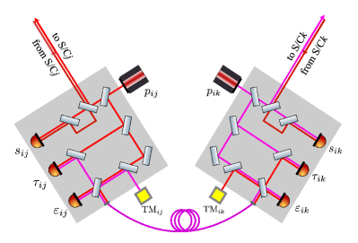
In Fig. 1, the , , and refer to the science interferometer, test-mass interferometer, and reference interferometer on each optical bench, respectively. With only considering laser noise, acceleration noise, and optical metrology noise, three interferometric measurements are expressed as
| (1) | ||||
where denotes laser noise on the optical bench of S/C pointing to S/C, represents optical path noise on the S/C facing , denotes the acceleration noise from test mass on the S/C pointing to , and is a time-delay operator, where is the arm length or propagation time from S/C to .
The expressions of TDI have been formulated in previous literature [4, 5, 6, 7, 9, 15, 13, 12]. As the fiducial TDI configuration, the expression of the first-generation Michelson-X could be written as
| (2) | ||||
where is a combination of interferometric measurements from S/C to S/C as defined in [74, 24, 18]. For the links in the counterclockwise directions (S/C2 S/C1, S/C3S/C2 and S/C1S/C3), the are
| (3) |
For the links in the clockwise directions, their expressions are slightly different,
| (4) |
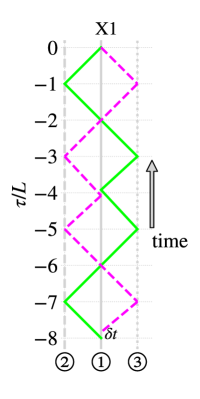
The corresponding second-generation TDI channels Michelson-X1 could be written as
| (5) | ||||
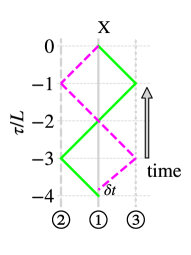
Their geometries are illustrated in Fig. 2, which will guide time-delay calculations in the following subsection.
For each TDI configuration, whether first-generation or second-generation, three ordinary channels could be constructed by cyclically permuting the indexes of three S/C. Then three (quasi-)orthogonal or optimal observables, denoted as (A, E, T), can be composed from ordinary observables using a linear combination [75, 76],
| (6) |
The A and E channels are expected to be science data streams capable of effectively detecting GW, while the T channel is expected to be GW-insensitive data and to characterize instrumental noises.
II.3 Algorithm for time delay calculation
Time delays are key quantities in TDI used to operate interferometric measurements as shown in Eqs. (1)-(5). Their calculations are implemented along the geometry of a TDI combination as illustrated in Fig. 2. Three vertical lines in Fig. 2 represent the trajectories of three S/C in the time direction. The horizontal separations between vertical lines indicate the spatial distances between S/C. The green and magenta lines show the two beams in the TDI link combination. The ticks on the y-axis represent the time delay with respect to the interferometric time . We select the Michelson-X observable to briefly explain the procedures of calculation, and a more detailed description can be found in [77]. The calculation starts from S/C1 at the earliest time point moving toward S/C2 at along the green line. The propagation time and position of laser arrival are determined at S/C2. The second step continues from S/C2 to S/C1 along the path of the green line to obtain the laser travel time and position of S/C1. When the calculation along green line reaches the S/C1 at the latest time point , the calculation continues along the magenta line in the backward time direction. The calculation stops at the initial sending S/C after completing a loop. Afterward, the time delays with respect to the latest time points are resolved from the result from each step, as well as the S/C positions.
During the propagation time calculation, additional relativistic time delays caused by gravitational fields are considered [78]. The time delay from the sending time at to the receiving time at is obtained by [79, 80],
| (7) |
where is the coordinate distance between the sender and receiver, is the speed of light, and is the relativistic time delay caused by gravitational field,
| (8) |
where is the gravitational constant, is the mass of the celestial body, and are unit vectors from the celestial body to the and positions, and and represent the radial distances of sender and receiver from the gravitating body, respectively. In the current calculation, the leading order of relativistic time delay caused by the gravitational field of the Sun is included, the effects from other planets are disregarded. Additionally, due to the orbital motion of the S/C, an iteration process is utilized to determine the arrival time and position of the receiver,
| (9) | ||||
The Chebyshev polynomial interpolation is employed to precisely determine the position of S/C at any given moment [81, 82].
In this calculation, the propagation time between S/C are computed numerically based on their orbit data. In a realistic scenario, the ranging time from sender to receiver would be estimated from measurements taken on S/C [83, 84, 85, 86, references therein]. In the simulation of the next section, the propagation time with a ranging error is taken into account to evaluate the residual laser noise in the TDI channels. For analysis of the GW signal from MBHB in Section IV, the uncertainties of arm lengths are expected to be trivial and negligible.
III Simulation of TDI
III.1 Simulation diagram
The diagram illustrating simulation and analysis process is presented in Fig. 3. The initial step involves selecting a mission with noise budgets and setting targeting source(s) is(are) set. In the second step, a TDI configuration is chosen, and the geometry of the link combination is generated accordingly. Subsequently, the time delays and positions of S/C are calculated by implementing algorithms in Section II. Based on the noise budgets, time-domain noises are generated for each component with a specified sample rate (In this work, we choose 4 Hz), assuming that the different noises are uncorrelated. TDI is then implemented by synthesizing these noises, and the data at each time point is obtained by using Lagrange interpolation [87, 88]. After TDI, the noise data are yielded with laser noise suppression.
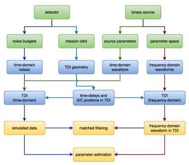
On the other hand, a GW signal from MBHB is simulated using a set of chosen parameters. The GW waveform in the time-domain is generated from the waveform model SEOBNRv4HM [89]. Subsequently, TDI is applied to the waveform in the SSB coordinate with TDB, and the responded waveform is computed considering the orbital motion of detector. The waveform is then injected into the noise data and yields the simulated data containing a GW signal. In the next step, the analysis is performed in the frequency domain. The frequency-domain waveforms are generated from a targeted parameter space using the reduced order model (ROM) of SEOBNRv4HM [90]. The waveforms multiplied by the response function of TDI are used for matched filtering to identify GW signs and infer the source parameters.
III.2 Noises
There are various types of observation noises for LISA [91], and our current focus is on laser frequency noise, acceleration noise, and optical metrology noise. The dominant laser frequency noise is generated by Nd:YAG lasers with a stability of , corresponding to an amplitude spectral density (ASD) of [1]. In this investigation, the first-generation and second-generation TDI Michelson observables are examined for laser noise suppressions. A ranging error between S/C is considered which includes a bias of 3 ns (0.9 m) and noise with a spectrum of [91, 92, 93].
Clock noise is assumed to be sufficiently canceled out by using the algorithm in [94] and is therefore ignored in current simulation. Both the acceleration noise and optical path noise are included with spectra
| (10) | ||||
where and are tunable amplitudes of noise for each optical bench, with and assigned to all components in current setups.
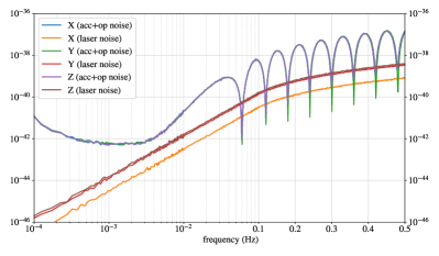
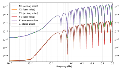
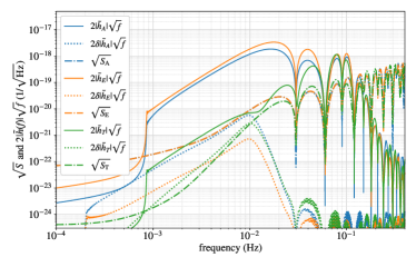
The examinations of laser noise suppressions in Michelson configurations are performed as tests, and the PSDs of residual laser noise are presented in Fig. 4. The results for the first-generation TDI channels, (X, Y, Z), are displayed in the upper plot, and the results for the second-generation TDI channels (X1, Y1, Z1) are depicted in the lower panel. Compared to the secondary noises including acceleration noise and optical metrology noise, residual laser noises in first-generation TDI channels are moderately lower at lower frequencies and slightly higher at characteristic frequencies in the current dataset. This level of laser noise is mainly limited by the path mismatches of two beams due to the orbital dynamics. For the second-generation TDI channels, the residual laser noise is significantly lower than secondary noises, and this level of suppression is subject to the ranging errors between S/C.
III.3 GW waveforms
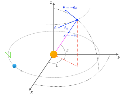
The conventions for waveform simulation in SSB coordinates are illustrated in Fig. 5 [96, 95]. For a source of MBHB, its location is described by the ecliptic longitude and ecliptic latitude . The propagation vector of GW will be
| (11) |
The orthogonal vectors in the longitude and latitude directions are defined as
| (12) | ||||
| (13) |
By defining the polarization angle , the principal directions are rotated from ,
| (14) | ||||
| (15) |
The tensors for and polarizations can be generated,
| (16) | ||||
| (17) |
Therefore, the GW responded in a laser link from the sender at to the receiver at could be expressed as
| (18) | ||||
where is the unit vector from sender to receiver, and represents the incoming GW signal from a source. The arrival time with the influence of GW could be obtained from
| (19) |
where is propagation time in the solar systems dynamics obtained from Eqs. (7)-(9), and the last term on the right side is the effects of GW. Approximating the wave propagation time as and position as , the GW at a given time point can be expressed as
| (20) |
The GW response in relative frequency deviation from sender to receiver could be written as [95]
| (21) |
With the responded GW in a single link, the time-domain waveform in a TDI channel will be
| (22) |
where the first term on the right side is cumulative effects of links from one (adding) beam, and the second term denotes the combination of another beam which will be subtracted from the first term. The response in the frequency domain could be expressed as
| (23) |
The frequency-domain waveform of TDI will be
| (24) |
The frequency evolution with time is calculated to obtain the instantaneous location of the detector and its response,
| (25) |
In contrast to Eq. (21), an approximation is usually applied , and the GW in the single link is written as
| (26) |
For the LISA mission, the velocity of the S/C in SSB coordinates will be 30 km/s, and the position of sender will deviate from the original location by 250 km during a transmission time of 8.33 s. Therefore, the approximation in Eq. (26) may introduce some inaccuracy in the calculation. We choose one source for simulation to examine the deviations between two algorithms given by Eqs. (21) and (26). The parameters for waveform simulation are shown in Table. 1.
| parameter | value | description |
|---|---|---|
| mass of primary BH in source frame | ||
| mass of secondary BH in source frame | ||
| 6791.8 Mpc | luminosity distance | |
| (redshift = 1.0 [97, 98]) | ||
| rad | inclination angle | |
| 4.603 rad | ecliptic longitude | |
| 0.314 rad | ecliptic latitude | |
| 0.55 rad | polarization angle | |
| 56.0 day | merger time at SSB center | |
| with respect to initial orbit time | ||
| reference phase | ||
| duration | 25 days | duration of chirp signal |
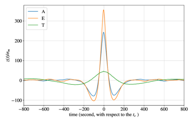
The simulated waveforms of the second-generation TDI Michelson configuration are shown in Fig. 6. In the upper panel, the time-domain waveforms in three optimal channels are present for the last 600 before the coalescence. The x-axis is the time in TDB relative to the arrival time of the merger signal at the SSB center. And the coalescence reaches the detector earlier than at the SSB center in current case. As depicted by the waveforms, the amplitudes and phases of waveforms are modulated by the TDI. The amplitudes of waveforms in A and E are significantly suppressed around s, corresponding to their lowest characteristic frequency, Hz. For higher frequencies, the wavelength of GW is shorter than , causing the mixed phase to cross one cycle in TDI. The different amplitudes of A and E also verify that two observables have different antenna patterns [99], despite two channels having identical averaged-sensitivities. The waveform in the T channel is noticeably canceled in low frequencies, and the amplitude is amplified with the increase of frequencies.
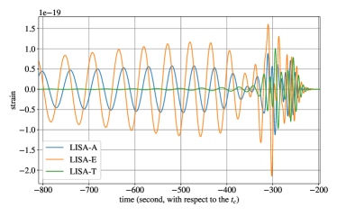
In the middle plot of Fig. 6, Fourier transforms are applied to the time-domain waveforms, as well as the differences between two waveforms (), generated from Eqs (21) and (26). These differences are depicted by the dotted lines, and the noise ASDs of TDI channels are also shown for comparison. The ASDs of A (blue dashed-dotted line) and E (orange dashed-dotted line) are equal and overlapped, and the T channel exhibits lower than the other two channels at lower frequencies and becomes comparable at high frequencies. For current source, the differences between two algorithms vary among three channels. In the T channel, the discrepancy could exceed its noise level within the frequency range of [1 mHz, 10 mHz]. The residual waveform in the A channel may be comparable to the noise level at certain frequencies, whereas the waveform difference in the E channel is one order of magnitude lower than its noise. The divergence levels of GW signals may vary with different sources. On the other hand, the waveforms in the frequency domain clearly show that GW signals are significantly suppressed by TDI around their characteristic frequencies ( for ).
In the lower panel of Fig. 6, in addition to the predominant harmonic mode of the GW, extra modes of waveform are simulated and plotted for the A channel. The dashed lines indicate the waveforms from time-domain simulation, and the solid lines represent the waveforms obtained by using the frequency-domain model. As shown by the curves, the waveforms exhibit good agreements in terms of amplitudes. However, the waveforms from time-domain and frequency-domain approximants are best fitted at different phases/times. As a result, their match decreases when matched filtering is implemented with integrated multiple harmonics. As a compromise, only the dominant mode is injected into the noise data to perform the analysis.
IV Analysis
The simulated data is synthesized by injecting the waveforms into the noise data. Initially, the ordinary data streams of the first-generation TDI observables (X, Y, Z) and the second-generation observables (X1, Y1, Z1) are generated. Then, the optimal data streams are composed using Eq. (6). The analysis strategy in current study comprises two steps, the first step involves matched filtering for signal identification, and the second step focuses on parameter inference for the binary.
IV.1 Identification of chirp signal
The fiducial strategy for identifying GW chirp signals involves filtering the data with a pre-built template bank [100, 101, 102, 40, and references therein]. The template bank should adequately cover the targeting parameter space with a required density [103, 104, 105, 106, and references therein]. Machine learning techniques have been applied to identify the chirp signals in advanced LIGO/Virgo data [107, 108]. For ground-based GW searches, chirp signals typically last seconds to dozens of seconds in the sensitive band of detectors, and the motion of detector with the Earth could be ignored. The template bank is built to cover the intrinsic parameters of the binary sources, such as masses and spins. However, for space-borne GW detectors, chirp signals could persist for days to months in their sensitive band, and the motion of interferometer could alter the response function to GWs. Moreover, TDI introduces the additional modulation into the observed signals. Therefore, the template bank may need to include extrinsic parameters to sufficiently match the observed signals. Weaving et al. [40] generated a template bank searched for MBHB in the LISA mock data, and verified the feasibility of the signal identification strategy. Given that the template bank searches are computing expensive, we only introduce the matched filtering algorithm here.
The matched filter is an optimal algorithm for identifying a GW signal with a known waveform. The output of the filtering can be expressed as [100]
| (27) |
where is the data in the frequency domain, is a waveform template, is the noise PSD of the data stream, and is a reference time which refers to coalescence time here. A normalization factor can be obtained for the template,
| (28) |
Then, the signal-to-noise ratio (SNR) of the matched filtering is given by
| (29) |
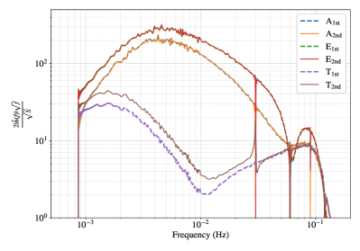
Using a frequency-domain waveforms modeled with fitted parameters in Section III.3, a matched filter is implemented to the optimal channels of the second-generation TDI Michelson, and the results are presented in the upper panel of Fig. 7. Among the three optimal channels, the E channel exhibits the highest SNR (), followed by the A channel with a lower SNR (). The T channel shows a significantly lower SNR () compared to the other two channels. Additionally, the SNR profile of the T channel is broader than that of other two channels, and this should be due to that its SNR is mainly contributed from lower frequencies.
An optimal SNR is defined for the template fully matching the signal in data,
| (30) | ||||
The ratio between the waveform and noise ASD partially reflect the SNR contribution across a log-scaled frequency range. The ratios for Michelson configuration from both first-generation and second-generation TDI are depicted in the lower panel of Fig. 7. As expected, the E channels exhibit the highest values among three observables, and the A channel is slightly lower than E for this instance. The A/E observables from both first-generation and second-generation TDI configurations are (nearly) identical, except at characteristic frequencies. Their largest SNR contributions are expected to occur in the frequency band around 5 mHz. However, noticeable differences are observed in the T channels between two different generations. As we have previously analyzed in [99, 51], benefiting from unequal arm interferometry, the T channels from Michelson TDI are more sensitive compared to the equal-arm case. The T channel may contain GW signals resulting from imperfect cancellation of the three ordinary channels (X, Y, Z) or (X1, Y1, Z1). The second-generation observables process more recurrent links than the first-generation, amplifying the effect of unequal arm length. Consequently, the SNR in the T channel of the second-generation is higher than that of the first-generation. On the other side, in these observables, especially for the second-generation, the ratios exhibit discontinuities at their characteristic frequencies, caused by the overestimated PSDs at these frequencies due to averaging.
IV.2 Parameter inference
Source parameters are inferred from the observed data by using Bayesian analysis. The posteriors of parameters are calculated from
| (31) |
where is prior probabilities of parameters. is the likelihood function of a set of parameters [109],
| (32) |
and is the correlation matrix of noises in selected TDI channels,
| (33) |
where is the observation time which is 30 days in this investigation, / are PSD or cross-spectral density of data streams which estimated by using algorithm detailed in [100]. For networks with multiple detectors, the joint log-likelihood is given by
| (34) |
The prior setups are shown in Table 2. Instead of inferring individual component masses (), the redshifted chirp mass and mass ratio are estimated. The prior of chirp mass is adjustable for different mass binaries, and the prior of mass ratio is set to be a range of [0.1, 0.2]. The prior ranges of these two parameters are set to be relatively smaller to reduce computing time, and it will not affect the final results. The luminosity distance uses a distribution in the comoving volume by using the cosmological parameters from Planck 2018 [97, 98]. The inclination follows a sinusoidal distribution, the sky location () is uniformly distributed in a spherical surface, the reference phase is evenly distributed in , and the coalescence time is uniformly sampled within 180 seconds with respect to the injected time. The Nested sampler [110, 111] is employed to perform the parameter inference.
| Variable | Prior | range | unit |
|---|---|---|---|
| uniform | |||
| uniform | [0.1, 0.2] | ||
| Comoving | [5000, 8000] | Mpc | |
| [0, ] | rad | ||
| uniform | [0, ] | rad | |
| [] | rad | ||
| uniform | [0, ] | rad | |
| uniform | [-180, +180] | second | |
| uniform | [0, ] | rad |
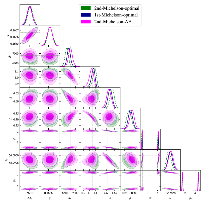
Three cases are executed for the first comparison with different TDI datasets: 1) three optimal channels (A, E, T) of first-generation Michelson, 2) three optimal channels from second-generation Michelson, and 3) two science channels from second-generation Michelson (A, E). The inferred distributions of parameters are shown in Fig. 8. The parameters inferred from three scenarios are moderately different. The distributions of the mass parameters are almost identical, while the distributions for extrinsic parameters vary with datasets. As aforementioned, the detectability of the T channel is sensitive to arm differences during the orbital motion, and the time-varying information could be averaged and discarded in the frequency-domain analysis. As a result, accurately inferring the signal in the T channel could be tricky or otherwise cause bias in estimation. As shown in the result, since the T channel from second-generation Michelson accumulates more SNR than it does in first-generation, the distributions of extrinsic parameters inferred from second-generation channels diverge from the injected values more than the first-generation, especially for the luminosity distance and longitude . After removing the T data stream, two science channels from the second-generation can constrain all parameters in sensible regions. As we also can see from the corner plot, the and are correlated as expected. The inclination not only degenerates with the distance but also the ecliptic latitude , and the longitude is correlated with arrival time . Both polarization angle and reference phase are inferred with bimodal distributions.
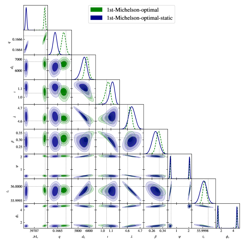
In another case, for a LISA-like mission, the orbital motion of interferometer will modulate the amplitude and phase of waveform. Hence, the effects of orbit dynamics should be taken into account when modeling TDI waveforms in the frequency-domain, especially for a long-duration signal. To access this impact, an inference with static constellation is performed using the first-generation Michelson optimal channels. The results are presented in Fig. 9. Compared to the dynamic model, the inferred values from the static model diverge from the true values, particularly for the intrinsic parameters, chirp mass and mass ratio , while the extrinsic parameters are still within the credible regions. Furthermore, the extrinsic parameters estimated from dynamic model exhibit better constraints with smaller uncertainties. One reason for this could be the better matched waveforms, and another reason could be that the motion of detector helps to resolve the location of source by demodulated response function.
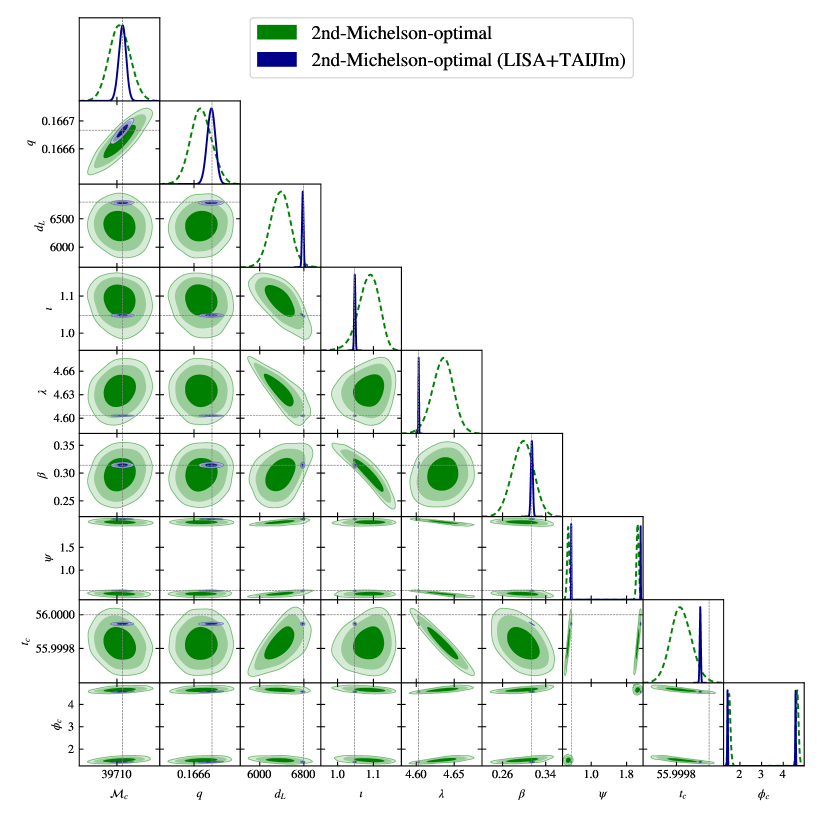
In principle, simulating and analyzing a variety of sources would be necessary to validate the analysis performance. However, this process would be computationally costly. To assess the analysis performance more rigorously, a more challenging case could be utilized to examine whether the parameters can be accurately inferred. As proposed in [55], the inclusion of the TAIJIm observatory in the network with LISA can significantly promote the determinations of parameters for MBHBs. By jointly analyzing simulated data for TAIJIm along with LISA, the result, shown by the blue regions in Fig. 10, indicates that all parameters can be inferred accurately with much smaller uncertainties. This suggests the correctness and robustness of analysis. Additionally, the joint data analysis also mitigates the inaccurate influence from the Michelson T channels and produces sensible distributions.
V Conclusion and discussion
In this work, we introduce a generic framework designed for simulating and analyzing TDI data. Our objectives include investigating key factors influencing TDI implementations, developing algorithms for GW analysis, and exploring the potential of alternative TDI observables. By utilizing numerical orbit simulations, the framework is capable of generating time-domain data comprising both noises and GW signals in TDI channels. Additionally, the current version of the framework incorporates parameter inference by matched filtering the modeled GW signal for MBHB. We specifically focus on simulating and analyzing a chirping GW signal using data streams from both first-generation and second-generation TDI Michelson configurations. The results validate the effectiveness of the framework and reveal the potential drawbacks of the fiducial Michelson configuration under scenarios with dynamic unequal arm lengths. Furthermore, we propose an alternative TDI configuration to mitigate the impacts of unequal arm and null frequencies in a companion paper [51].
LISA is chosen as the typical mission for demonstrating the simulation and analysis in this study, and the framework is also applicable to other space-based GW missions employing TDI. The validation of these processes are carried out by selecting MBHBs, which are the primary targets of LISA. In the data analysis, harmonic modes of GWs beyond the are omitted, although incorporating additional modes could improve parameter inference. In addition, the Doppler effect resulting from detector motion is disregarded, as the modulation is expected to be insignificant for a one-month chirp signal at current SNR levels. However, this modulation could become significant and should be considered for less massive binaries with longer durations, such as stellar-mass compact binaries. Extended analysis incorporating greater completeness will be pursued in future work.
A challenge in GW observations in the milli-Hz band is the simultaneous detection of various sources, both of the same and different types, leading to heavily overlapped signals. Additionally, instrumental noises may vary over time, and observed data may not be continuous. As the framework evolves, these effects will be integrated into the simulation, warranting comprehensive investigations into their impacts on GW analysis. Moreover, networks with multiple detectors show promise for boosting GW detections in space [112], and the joint analysis could offer significant benefits, as tentatively explored in this study. Relevant simulations and analyses will be conducted in future work.
Acknowledgements.
GW thanks Alex Nitz, Runqiu Liu, and Minghui Du for helpful communications and discussions. GW was supported by the National Key R&D Program of China under Grant No. 2021YFC2201903, and NSFC No. 12003059. This work made use of the High Performance Computing Resource in the Core Facility for Advanced Research Computing at Shanghai Astronomical Observatory. This work are performed by using the python packages [113], [114], [115], PyCBC [101, 116], LALSuite [117, 118], [98], [119], [110] and [111], and the plots are make by utilizing [120], [121] and [122].References
- Amaro-Seoane et al. [2017] P. Amaro-Seoane, H. Audley, S. Babak, and et al (LISA Team), Laser Interferometer Space Antenna, arXiv e-prints , arXiv:1702.00786 (2017).
- Colpi et al. [2024] M. Colpi et al., LISA Definition Study Report, (2024), arXiv:2402.07571 [astro-ph.CO] .
- Ni et al. [1997] W.-T. Ni, J.-T. Shy, S.-M. Tseng, X. Xu, H.-C. Yeh, W.-Y. Hsu, W.-L. Liu, S.-D. Tzeng, P. Fridelance, E. Samain, D. Lee, Z.-Y. Su, and A.-M. Wu, Progress in mission concept study and laboratory development for the ASTROD (Astrodynamical Space Test of Relativity using Optical Devices), in Small Spacecraft, Space Environments, and Instrumentation Technologies, Society of Photo-Optical Instrumentation Engineers (SPIE) Conference Series, Vol. 3116, edited by F. A. Allahdadi, E. K. Casani, and T. D. Maclay (1997) pp. 105–116.
- Armstrong et al. [1999] J. W. Armstrong, F. B. Estabrook, and M. Tinto, Time-Delay Interferometry for Space-based Gravitational Wave Searches, Astrophys. J. 527, 814 (1999).
- Estabrook et al. [2000] F. B. Estabrook, M. Tinto, and J. W. Armstrong, Time-delay analysis of LISA gravitational wave data: Elimination of spacecraft motion effects, Phys. Rev. D 62, 042002 (2000).
- Armstrong et al. [2001] J. W. Armstrong, F. B. Estabrook, and M. Tinto, Sensitivities of alternate LISA configurations, Classical and Quantum Gravity 18, 4059 (2001).
- Larson et al. [2002] S. L. Larson, R. W. Hellings, and W. A. Hiscock, Unequal arm space borne gravitational wave detectors, Phys. Rev. D 66, 062001 (2002), arXiv:gr-qc/0206081 .
- Dhurandhar et al. [2002] S. V. Dhurandhar, K. Rajesh Nayak, and J. Y. Vinet, Algebraic approach to time-delay data analysis for LISA, Phys. Rev. D 65, 102002 (2002), arXiv:gr-qc/0112059 [gr-qc] .
- Tinto et al. [2003] M. Tinto, D. A. Shaddock, J. Sylvestre, and J. W. Armstrong, Implementation of time-delay interferometry for LISA, Phys. Rev. D 67, 122003 (2003), arXiv:gr-qc/0303013 [gr-qc] .
- Vallisneri [2005a] M. Vallisneri, Synthetic LISA: Simulating time delay interferometry in a model LISA, Phys. Rev. D 71, 022001 (2005a), arXiv:gr-qc/0407102 [gr-qc] .
- Petiteau et al. [2008] A. Petiteau, G. Auger, H. Halloin, O. Jeannin, E. Plagnol, S. Pireaux, T. Regimbau, and J.-Y. Vinet, LISACode: A scientific simulator of LISA, Phys. Rev. D 77, 023002 (2008), arXiv:0802.2023 [gr-qc] .
- Tinto and Dhurandhar [2021] M. Tinto and S. V. Dhurandhar, Time-delay interferometry, Living Rev. Rel. 24, 1 (2021).
- Shaddock et al. [2003] D. A. Shaddock, M. Tinto, F. B. Estabrook, and J. Armstrong, Data combinations accounting for LISA spacecraft motion, Phys. Rev. D 68, 061303 (2003), arXiv:gr-qc/0307080 .
- Cornish and Hellings [2003] N. J. Cornish and R. W. Hellings, The Effects of orbital motion on LISA time delay interferometry, Class. Quant. Grav. 20, 4851 (2003), arXiv:gr-qc/0306096 [gr-qc] .
- Tinto et al. [2004] M. Tinto, F. B. Estabrook, and J. Armstrong, Time delay interferometry with moving spacecraft arrays, Phys. Rev. D 69, 082001 (2004), arXiv:gr-qc/0310017 .
- Vallisneri [2005b] M. Vallisneri, Geometric time delay interferometry, Phys. Rev. D 72, 042003 (2005b), [Erratum: Phys. Rev. D 76, 109903(2007)], arXiv:gr-qc/0504145 [gr-qc] .
- Dhurandhar et al. [2010] S. Dhurandhar, K. Nayak, and J. Vinet, Time Delay Interferometry for LISA with one arm dysfunctional, Class. Quant. Grav. 27, 135013 (2010), arXiv:1001.4911 [gr-qc] .
- Tinto and Hartwig [2018] M. Tinto and O. Hartwig, Time-Delay Interferometry and Clock-Noise Calibration, Phys. Rev. D 98, 042003 (2018), arXiv:1807.02594 [gr-qc] .
- Bayle et al. [2019] J.-B. Bayle, M. Lilley, A. Petiteau, and H. Halloin, Effect of filters on the time-delay interferometry residual laser noise for LISA, Phys. Rev. D 99, 084023 (2019), arXiv:1811.01575 [astro-ph.IM] .
- Muratore et al. [2020] M. Muratore, D. Vetrugno, and S. Vitale, Revisitation of time delay interferometry combinations that suppress laser noise in LISA, arXiv e-prints (2020), arXiv:2001.11221 [astro-ph.IM] .
- Vallisneri et al. [2020] M. Vallisneri, J.-B. Bayle, S. Babak, and A. Petiteau, TDI-infinity: time-delay interferometry without delays, (2020), arXiv:2008.12343 [gr-qc] .
- Cornish and Rubbo [2003] N. J. Cornish and L. J. Rubbo, The LISA response function, Phys. Rev. D 67, 022001 (2003), [Erratum: Phys.Rev.D 67, 029905 (2003)], arXiv:gr-qc/0209011 .
- Rubbo et al. [2004] L. J. Rubbo, N. J. Cornish, and O. Poujade, Forward modeling of space borne gravitational wave detectors, Phys. Rev. D 69, 082003 (2004), arXiv:gr-qc/0311069 .
- Otto [2015] M. Otto, Time-Delay Interferometry Simulations for the Laser Interferometer Space Antenna (2015).
- Petiteau et al. [2008] A. Petiteau, G. Auger, H. Halloin, O. Jeannin, E. Plagnol, S. Pireaux, T. Regimbau, and J.-Y. Vinet, LISACode: A Scientific simulator of LISA, Phys. Rev. D 77, 023002 (2008), arXiv:0802.2023 [gr-qc] .
- Bayle et al. [2022] J.-B. Bayle, O. Hartwig, A. Petiteau, and M. Lilley, Lisanode (2022).
- Staab et al. [2023a] M. Staab, J.-B. Bayle, and O. Hartwig, Pytdi (2023a).
- Bayle et al. [2023a] J.-B. Bayle, Q. Baghi, A. Renzini, and M. Le Jeune, Lisa gw response (2023a).
- Bayle et al. [2023b] J.-B. Bayle, O. Hartwig, and M. Staab, Lisa instrument (2023b).
- de Vine et al. [2010] G. de Vine, B. Ware, K. McKenzie, R. E. Spero, W. M. Klipstein, and D. A. Shaddock, Experimental Demonstration of Time-Delay Interferometry for the Laser Interferometer Space Antenna, Phys. Rev. Lett. 104, 211103 (2010), arXiv:1005.2176 [astro-ph.IM] .
- Vinckier et al. [2020] Q. Vinckier, M. Tinto, I. Grudinin, D. Rieländer, and N. Yu, Experimental demonstration of time-delay interferometry with optical frequency comb, Phys. Rev. D 102, 062002 (2020).
- Cornish and Shuman [2020] N. J. Cornish and K. Shuman, Black Hole Hunting with LISA, Phys. Rev. D 101, 124008 (2020), arXiv:2005.03610 [gr-qc] .
- Marsat et al. [2021] S. Marsat, J. G. Baker, and T. Dal Canton, Exploring the Bayesian parameter estimation of binary black holes with LISA, Phys. Rev. D 103, 083011 (2021), arXiv:2003.00357 [gr-qc] .
- Katz [2022] M. L. Katz, Fully automated end-to-end pipeline for massive black hole binary signal extraction from LISA data, Phys. Rev. D 105, 044055 (2022), arXiv:2111.01064 [gr-qc] .
- Pratten et al. [2023] G. Pratten, A. Klein, C. J. Moore, H. Middleton, N. Steinle, P. Schmidt, and A. Vecchio, LISA science performance in observations of short-lived signals from massive black hole binary coalescences, Phys. Rev. D 107, 123026 (2023), arXiv:2212.02572 [gr-qc] .
- Karnesis et al. [2023] N. Karnesis, M. L. Katz, N. Korsakova, J. R. Gair, and N. Stergioulas, Eryn : A multi-purpose sampler for Bayesian inference, Mon. Not. Roy. Astron. Soc. 526, 4814 (2023), arXiv:2303.02164 [astro-ph.IM] .
- Katz et al. [2020] M. L. Katz, S. Marsat, A. J. K. Chua, S. Babak, and S. L. Larson, GPU-accelerated massive black hole binary parameter estimation with LISA, Phys. Rev. D 102, 023033 (2020), arXiv:2005.01827 [gr-qc] .
- Cornish [2021] N. J. Cornish, Heterodyned likelihood for rapid gravitational wave parameter inference, Phys. Rev. D 104, 104054 (2021), arXiv:2109.02728 [gr-qc] .
- Zackay et al. [2018] B. Zackay, L. Dai, and T. Venumadhav, Relative Binning and Fast Likelihood Evaluation for Gravitational Wave Parameter Estimation, (2018), arXiv:1806.08792 [astro-ph.IM] .
- Weaving et al. [2023] C. R. Weaving, L. K. Nuttall, I. W. Harry, S. Wu, and A. Nitz, Adapting the PyCBC pipeline to find and infer the properties of gravitational waves from massive black hole binaries in LISA, (2023), arXiv:2306.16429 [astro-ph.IM] .
- Williams et al. [2021] M. J. Williams, J. Veitch, and C. Messenger, Nested sampling with normalizing flows for gravitational-wave inference, Phys. Rev. D 103, 103006 (2021), arXiv:2102.11056 [gr-qc] .
- Gabbard et al. [2022] H. Gabbard, C. Messenger, I. S. Heng, F. Tonolini, and R. Murray-Smith, Bayesian parameter estimation using conditional variational autoencoders for gravitational-wave astronomy, Nature Phys. 18, 112 (2022), arXiv:1909.06296 [astro-ph.IM] .
- Langendorff et al. [2023] J. Langendorff, A. Kolmus, J. Janquart, and C. Van Den Broeck, Normalizing Flows as an Avenue to Studying Overlapping Gravitational Wave Signals, Phys. Rev. Lett. 130, 171402 (2023), arXiv:2211.15097 [gr-qc] .
- Dax et al. [2023] M. Dax, S. R. Green, J. Gair, M. Pürrer, J. Wildberger, J. H. Macke, A. Buonanno, and B. Schölkopf, Neural Importance Sampling for Rapid and Reliable Gravitational-Wave Inference, Phys. Rev. Lett. 130, 171403 (2023), arXiv:2210.05686 [gr-qc] .
- Ruan et al. [2023a] W.-H. Ruan, H. Wang, C. Liu, and Z.-K. Guo, Rapid search for massive black hole binary coalescences using deep learning, Phys. Lett. B 841, 137904 (2023a), arXiv:2111.14546 [astro-ph.IM] .
- Ruan et al. [2023b] W. Ruan, H. Wang, C. Liu, and Z. Guo, Parameter Inference for Coalescing Massive Black Hole Binaries Using Deep Learning, Universe 9, 407 (2023b), arXiv:2307.14844 [astro-ph.IM] .
- Du et al. [2023] M. Du, B. Liang, H. Wang, P. Xu, Z. Luo, and Y. Wu, Advancing Space-Based Gravitational Wave Astronomy: Rapid Detection and Parameter Estimation Using Normalizing Flows, (2023), arXiv:2308.05510 [astro-ph.IM] .
- Sun et al. [2023] T.-Y. Sun, C.-Y. Xiong, S.-J. Jin, Y.-X. Wang, J.-F. Zhang, and X. Zhang, Efficient parameter inference for gravitational wave signals in the presence of transient noises using normalizing flow, (2023), arXiv:2312.08122 [gr-qc] .
- Littenberg et al. [2020] T. Littenberg, N. Cornish, K. Lackeos, and T. Robson, Global Analysis of the Gravitational Wave Signal from Galactic Binaries, Phys. Rev. D 101, 123021 (2020), arXiv:2004.08464 [gr-qc] .
- Littenberg and Cornish [2023] T. B. Littenberg and N. J. Cornish, Prototype global analysis of LISA data with multiple source types, Phys. Rev. D 107, 063004 (2023), arXiv:2301.03673 [gr-qc] .
- Wang [2024] G. Wang, Time delay interferometry with minimal null frequencies, (2024), arXiv:2403.xxxx [gr-qc] .
- Hu and Wu [2017] W.-R. Hu and Y.-L. Wu, The Taiji Program in Space for gravitational wave physics and the nature of gravity, Natl. Sci. Rev. 4, 685 (2017).
- Ruan et al. [2020] W.-H. Ruan, C. Liu, Z.-K. Guo, Y.-L. Wu, and R.-G. Cai, The LISA-Taiji network, Nature Astron. 4, 108 (2020), arXiv:2002.03603 [gr-qc] .
- Wang et al. [2020] G. Wang, W.-T. Ni, W.-B. Han, S.-C. Yang, and X.-Y. Zhong, Numerical simulation of sky localization for LISA-TAIJI joint observation, Phys. Rev. D 102, 024089 (2020), arXiv:2002.12628 .
- Wang et al. [2021a] G. Wang, W.-T. Ni, W.-B. Han, P. Xu, and Z. Luo, Alternative LISA-TAIJI networks, Phys. Rev. D 104, 024012 (2021a), arXiv:2105.00746 [gr-qc] .
- Wang and Han [2021] G. Wang and W.-B. Han, Alternative LISA-TAIJI networks: Detectability of the isotropic stochastic gravitational wave background, Phys. Rev. D 104, 104015 (2021), arXiv:2108.11151 [gr-qc] .
- Dhurandhar et al. [2005] S. V. Dhurandhar, K. R. Nayak, S. Koshti, and J. Y. Vinet, Fundamentals of the LISA stable flight formation, Class. Quant. Grav. 22, 481 (2005), arXiv:gr-qc/0410093 [gr-qc] .
- Nayak et al. [2006] K. R. Nayak, S. Koshti, S. V. Dhurandhar, and J. Y. Vinet, On the minimum flexing of LISA’s arms, Class. Quant. Grav. 23, 1763 (2006).
- Wang and Ni [2013a] G. Wang and W.-T. Ni, Numermcal simulation of time delay interferometry for NGO/eLISA, Class. Quant. Grav. 30, 065011 (2013a), arXiv:1204.2125 [gr-qc] .
- Dhurandhar et al. [2013] S. V. Dhurandhar, W. T. Ni, and G. Wang, Numerical simulation of time delay interferometry for a LISA-like mission with the simplification of having only one interferometer, Adv. Space Res. 51, 198 (2013), arXiv:1102.4965 [gr-qc] .
- Wang and Ni [2019] G. Wang and W.-T. Ni, Numerical simulation of time delay interferometry for TAIJI and new LISA, Res. Astron. Astrophys. 19, 058 (2019), arXiv:1707.09127 [astro-ph.IM] .
- Ni [2013a] W.-T. Ni, Dark energy, co-evolution of massive black holes with galaxies, and ASTROD-GW, Adv. Space Res. 51, 525 (2013a), arXiv:1104.5049 [astro-ph.CO] .
- Ni [2013b] W.-T. Ni, ASTROD-GW: Overview and Progress, Int. J. Mod. Phys. D 22, 1341004 (2013b), arXiv:1212.2816 [astro-ph.IM] .
- Wang [2011] G. Wang, Time-delay Interferometry for ASTROD-GW (2011).
- Wang and Ni [2012] G. Wang and W.-T. Ni, Time-delay Interferometry for ASTROD-GW, Chin. Astron. Astrophys. 36, 211 (2012), and references therein.
- Wang and Ni [2015] G. Wang and W.-T. Ni, Orbit optimization and time delay interferometry for inclined ASTROD-GW formation with half-year precession-period, Chin. Phys. B24, 059501 (2015), arXiv:1409.4162 [gr-qc] .
- Wang and Ni [2013b] G. Wang and W.-T. Ni, Orbit optimization for ASTROD-GW and its time delay interferometry with two arms using CGC ephemeris, Chin. Phys. B22, 049501 (2013b), arXiv:1205.5175 [gr-qc] .
- Ni et al. [2020] W.-T. Ni, G. Wang, and A.-M. Wu, Astrodynamical middle-frequency interferometric gravitational wave observatory AMIGO: Mission concept and orbit design, Int. J. Mod. Phys. D 29, 1940007 (2020), arXiv:1909.04995 [gr-qc] .
- Folkner et al. [2014] W. M. Folkner, J. G. Williams, D. H. Boggs, R. S. Park, and P. Kuchynka, The Planetary and Lunar Ephemerides DE430 and DE431 (2014), iPN Progress Report 42-196.
- Park et al. [2021] R. S. Park, W. M. Folkner, J. G. Williams, and D. H. Boggs, The JPL Planetary and Lunar Ephemerides DE440 and DE441, Astron. J. 161, 105 (2021).
- Soffel et al. [2003] M. Soffel et al., The IAU 2000 resolutions for astrometry, celestial mechanics and metrology in the relativistic framework: Explanatory supplement, Astron. J. 126, 2687 (2003), arXiv:astro-ph/0303376 .
- Yang et al. [2022] P. Yang, Y. Huang, P. Li, H. Wang, M. Fan, S. Liu, Q. Shan, S. Qin, and Q. Liu, Orbit determination of china’s first mars probe tianwen-1 during interplanetary cruise, Advances in Space Research 69, 1060 (2022).
- Li et al. [2024] P. Li, Y. Huang, and X. Hu, (2024), in preparation.
- Otto et al. [2012] M. Otto, G. Heinzel, and K. Danzmann, TDI and clock noise removal for the split interferometry configuration of LISA, Class. Quant. Grav. 29, 205003 (2012).
- Prince et al. [2002] T. A. Prince, M. Tinto, S. L. Larson, and J. W. Armstrong, The LISA optimal sensitivity, Phys. Rev. D 66, 122002 (2002), arXiv:gr-qc/0209039 [gr-qc] .
- Vallisneri et al. [2008] M. Vallisneri, J. Crowder, and M. Tinto, Sensitivity and parameter-estimation precision for alternate LISA configurations, Class. Quant. Grav. 25, 065005 (2008), arXiv:0710.4369 [gr-qc] .
- Wang et al. [2021b] G. Wang, W.-T. Ni, W.-B. Han, and C.-F. Qiao, Algorithm for time-delay interferometry numerical simulation and sensitivity investigation, Phys. Rev. D 103, 122006 (2021b), arXiv:2010.15544 [gr-qc] .
- Ashby and Bender [2008] N. Ashby and P. L. Bender, Measurement of the Shapiro Time Delay Between Drag-Free Spacecraft, Astrophys. Space Sci. Libr. 349, 219 (2008).
- Shapiro [1964] I. I. Shapiro, Fourth Test of General Relativity, Phys. Rev. Lett. 13, 789 (1964).
- Kopeikin [2009] S. M. Kopeikin, Post-Newtonian limitations on measurement of the PPN parameters caused by motion of gravitating bodies, Mon. Not. Roy. Astron. Soc. 399, 1539 (2009), arXiv:0809.3433 [gr-qc] .
- Newhall [1989] X. X. Newhall, Numerical Representation of Planetary Ephemerides, Celestial Mechanics 45, 305 (1989).
- Li and Tian [2004] G. Li and L. Tian, PMOE 2003 Planetary ephemeris framework (V) creating and using of ephemeris files, Publication of Purple Mountain Astronomical Observatory 23, 160 (2004).
- Heinzel et al. [2011] G. Heinzel, J. J. Esteban, S. Barke, M. Otto, Y. Wang, A. F. Garcia, and K. Danzmann, Auxiliary functions of the LISA laser link: Ranging, clock noise transfer and data communication, Class. Quant. Grav. 28, 094008 (2011).
- Reinhardt et al. [2023] J. N. Reinhardt, M. Staab, K. Yamamoto, J.-B. Bayle, A. Hees, O. Hartwig, K. Wiesner, and G. Heinzel, Ranging Sensor Fusion in LISA Data Processing: Treatment of Ambiguities, Noise, and On-Board Delays in LISA Ranging Observables, (2023), arXiv:2307.05204 [gr-qc] .
- Tinto et al. [2005] M. Tinto, M. Vallisneri, and J. W. Armstrong, TDIR: Time-delay interferometric ranging for space-borne gravitational-wave detectors, Phys. Rev. D 71, 041101 (2005), arXiv:gr-qc/0410122 .
- Page and Littenberg [2023] J. Page and T. B. Littenberg, Bayesian time delay interferometry for orbiting LISA: Accounting for the time dependence of spacecraft separations, Phys. Rev. D 108, 044065 (2023), arXiv:2305.14186 [gr-qc] .
- Shaddock et al. [2004] D. A. Shaddock, B. Ware, R. E. Spero, and M. Vallisneri, Post-processed time-delay interferometry for LISA, Phys. Rev. D 70, 081101 (2004), arXiv:gr-qc/0406106 .
- Bayle [2019] J.-B. Bayle, Simulation and Data Analysis for LISA : Instrumental Modeling, Time-Delay Interferometry, Noise-Reduction Permormance Study, and Discrimination of Transient Gravitational Signals, Ph.D. thesis, Paris U. VII, APC (2019).
- Bohé et al. [2017] A. Bohé et al., Improved effective-one-body model of spinning, nonprecessing binary black holes for the era of gravitational-wave astrophysics with advanced detectors, Phys. Rev. D 95, 044028 (2017), arXiv:1611.03703 [gr-qc] .
- Cotesta et al. [2020] R. Cotesta, S. Marsat, and M. Pürrer, Frequency domain reduced order model of aligned-spin effective-one-body waveforms with higher-order modes, Phys. Rev. D 101, 124040 (2020), arXiv:2003.12079 [gr-qc] .
- Bayle and Hartwig [2023] J.-B. Bayle and O. Hartwig, Unified model for the LISA measurements and instrument simulations, Phys. Rev. D 107, 083019 (2023), arXiv:2212.05351 [gr-qc] .
- Hartwig et al. [2022] O. Hartwig, J.-B. Bayle, M. Staab, A. Hees, M. Lilley, and P. Wolf, Time-delay interferometry without clock synchronization, Phys. Rev. D 105, 122008 (2022), arXiv:2202.01124 [gr-qc] .
- Staab et al. [2023b] M. Staab, M. Lilley, J.-B. Bayle, and O. Hartwig, Laser noise residuals in LISA from onboard processing and time-delay interferometry, (2023b), arXiv:2306.11774 [astro-ph.IM] .
- Hartwig and Bayle [2021] O. Hartwig and J.-B. Bayle, Clock-jitter reduction in LISA time-delay interferometry combinations, Phys. Rev. D 103, 123027 (2021), arXiv:2005.02430 [astro-ph.IM] .
- Katz et al. [2022] M. L. Katz, J.-B. Bayle, A. J. K. Chua, and M. Vallisneri, Assessing the data-analysis impact of LISA orbit approximations using a GPU-accelerated response model, Phys. Rev. D 106, 103001 (2022), arXiv:2204.06633 [gr-qc] .
- Vallisneri and Galley [2012] M. Vallisneri and C. R. Galley, Non-sky-averaged sensitivity curves for space-based gravitational-wave observatories, Class. Quant. Grav. 29, 124015 (2012), arXiv:1201.3684 [gr-qc] .
- Aghanim et al. [2020] N. Aghanim et al. (Planck), Planck 2018 results. VI. Cosmological parameters, Astron. Astrophys. 641, A6 (2020), [Erratum: Astron.Astrophys. 652, C4 (2021)], arXiv:1807.06209 [astro-ph.CO] .
- Robitaille et al. [2013] T. P. Robitaille et al. (Astropy), Astropy: A Community Python Package for Astronomy, Astron. Astrophys. 558, A33 (2013), arXiv:1307.6212 [astro-ph.IM] .
- Wang and Ni [2023] G. Wang and W.-T. Ni, Revisiting time delay interferometry for unequal-arm LISA and TAIJI, Phys. Scripta 98, 075005 (2023), arXiv:2008.05812 [gr-qc] .
- Allen et al. [2012] B. Allen, W. G. Anderson, P. R. Brady, D. A. Brown, and J. D. E. Creighton, FINDCHIRP: An Algorithm for detection of gravitational waves from inspiraling compact binaries, Phys. Rev. D 85, 122006 (2012), arXiv:gr-qc/0509116 .
- Usman et al. [2016] S. A. Usman et al., The PyCBC search for gravitational waves from compact binary coalescence, Class. Quant. Grav. 33, 215004 (2016), arXiv:1508.02357 [gr-qc] .
- Nitz et al. [2017] A. H. Nitz, T. Dent, T. Dal Canton, S. Fairhurst, and D. A. Brown, Detecting binary compact-object mergers with gravitational waves: Understanding and Improving the sensitivity of the PyCBC search, Astrophys. J. 849, 118 (2017), arXiv:1705.01513 [gr-qc] .
- Babak et al. [2013] S. Babak et al., Searching for gravitational waves from binary coalescence, Phys. Rev. D 87, 024033 (2013), arXiv:1208.3491 [gr-qc] .
- Brown et al. [2012] D. A. Brown, I. Harry, A. Lundgren, and A. H. Nitz, Detecting binary neutron star systems with spin in advanced gravitational-wave detectors, Phys. Rev. D 86, 084017 (2012), arXiv:1207.6406 [gr-qc] .
- Dal Canton et al. [2014] T. Dal Canton et al., Implementing a search for aligned-spin neutron star-black hole systems with advanced ground based gravitational wave detectors, Phys. Rev. D 90, 082004 (2014), arXiv:1405.6731 [gr-qc] .
- Sakon et al. [2022] S. Sakon et al., Template bank for compact binary mergers in the fourth observing run of Advanced LIGO, Advanced Virgo, and KAGRA, (2022), arXiv:2211.16674 [gr-qc] .
- Gabbard et al. [2018] H. Gabbard, M. Williams, F. Hayes, and C. Messenger, Matching matched filtering with deep networks for gravitational-wave astronomy, Phys. Rev. Lett. 120, 141103 (2018), arXiv:1712.06041 [astro-ph.IM] .
- Schäfer et al. [2023] M. B. Schäfer et al., First machine learning gravitational-wave search mock data challenge, Phys. Rev. D 107, 023021 (2023), arXiv:2209.11146 [astro-ph.IM] .
- Romano and Cornish [2017] J. D. Romano and N. J. Cornish, Detection methods for stochastic gravitational-wave backgrounds: a unified treatment, Living Rev. Rel. 20, 2 (2017), arXiv:1608.06889 [gr-qc] .
- Feroz et al. [2009] F. Feroz, M. P. Hobson, and M. Bridges, MultiNest: an efficient and robust Bayesian inference tool for cosmology and particle physics, Mon. Not. Roy. Astron. Soc. 398, 1601 (2009), arXiv:0809.3437 [astro-ph] .
- Buchner et al. [2014] J. Buchner, A. Georgakakis, K. Nandra, L. Hsu, C. Rangel, M. Brightman, A. Merloni, M. Salvato, J. Donley, and D. Kocevski, X-ray spectral modelling of the AGN obscuring region in the CDFS: Bayesian model selection and catalogue, Astron. Astrophys. 564, A125 (2014), arXiv:1402.0004 [astro-ph.HE] .
- Cai et al. [2023] R.-G. Cai, Z.-K. Guo, B. Hu, C. Liu, Y. Lu, W.-T. Ni, W.-H. Ruan, N. Seto, G. Wang, and Y.-L. Wu, On networks of space-based gravitational-wave detectors, (2023), arXiv:2305.04551 [gr-qc] .
- Harris et al. [2020] C. R. Harris, K. J. Millman, S. J. van der Walt, R. Gommers, P. Virtanen, D. Cournapeau, E. Wieser, J. Taylor, S. Berg, N. J. Smith, R. Kern, M. Picus, S. Hoyer, M. H. van Kerkwijk, M. Brett, A. Haldane, J. F. del Río, M. Wiebe, P. Peterson, P. Gérard-Marchant, K. Sheppard, T. Reddy, W. Weckesser, H. Abbasi, C. Gohlke, and T. E. Oliphant, Array programming with NumPy, Nature 585, 357 (2020).
- Virtanen et al. [2020] P. Virtanen, R. Gommers, T. E. Oliphant, M. Haberland, T. Reddy, D. Cournapeau, E. Burovski, P. Peterson, W. Weckesser, J. Bright, S. J. van der Walt, M. Brett, J. Wilson, K. J. Millman, N. Mayorov, A. R. J. Nelson, E. Jones, R. Kern, E. Larson, C. J. Carey, İ. Polat, Y. Feng, E. W. Moore, J. VanderPlas, D. Laxalde, J. Perktold, R. Cimrman, I. Henriksen, E. A. Quintero, C. R. Harris, A. M. Archibald, A. H. Ribeiro, F. Pedregosa, P. van Mulbregt, and SciPy 1.0 Contributors, SciPy 1.0: Fundamental Algorithms for Scientific Computing in Python, Nature Methods 17, 261 (2020).
- pandas development team [2020] T. pandas development team, pandas-dev/pandas: Pandas (2020).
- Biwer et al. [2019] C. M. Biwer, C. D. Capano, S. De, M. Cabero, D. A. Brown, A. H. Nitz, and V. Raymond, PyCBC Inference: A Python-based parameter estimation toolkit for compact binary coalescence signals, Publ. Astron. Soc. Pac. 131, 024503 (2019), arXiv:1807.10312 [astro-ph.IM] .
- LIGO Scientific Collaboration et al. [2018] LIGO Scientific Collaboration, Virgo Collaboration, and KAGRA Collaboration, LVK Algorithm Library - LALSuite, Free software (GPL) (2018).
- Wette [2020] K. Wette, SWIGLAL: Python and Octave interfaces to the LALSuite gravitational-wave data analysis libraries, SoftwareX 12, 100634 (2020).
- Ashton et al. [2019] G. Ashton et al., BILBY: A user-friendly Bayesian inference library for gravitational-wave astronomy, Astrophys. J. Suppl. 241, 27 (2019), arXiv:1811.02042 [astro-ph.IM] .
- Hunter [2007] J. D. Hunter, Matplotlib: A 2D Graphics Environment, Comput. Sci. Eng. 9, 90 (2007).
- Lewis [2019] A. Lewis, GetDist: a Python package for analysing Monte Carlo samples, (2019), arXiv:1910.13970 [astro-ph.IM] .
- [122] http://www.gwoptics.org/ComponentLibrary/.