Statistical Mechanics of Dynamical System Identification

Abstract

Recovering dynamical equations from observed noisy data is the central challenge of system identification. We develop a statistical mechanical approach to analyze sparse equation discovery algorithms, which typically balance data fit and parsimony through a trial-and-error selection of hyperparameters. In this framework, statistical mechanics offers tools to analyze the interplay between complexity and fitness, in analogy to that done between entropy and energy. To establish this analogy, we define the optimization procedure as a two-level Bayesian inference problem that separates variable selection from coefficient values and enables the computation of the posterior parameter distribution in closed form. A key advantage of employing statistical mechanical concepts, such as free energy and the partition function, is in the quantification of uncertainty, especially in in the low-data limit; frequently encountered in real-world applications. As the data volume increases, our approach mirrors the thermodynamic limit, leading to distinct sparsity- and noise-induced phase transitions that delineate correct from incorrect identification. This perspective of sparse equation discovery, is versatile and can be adapted to various other equation discovery algorithms.

I Introduction

Identifying dynamical models from data represents a critical challenge in a world inundated with time-series data, yet lacking the tools for accurate and robust modeling. This is the central task of modern system identification [1]. Traditional methods of constructing ordinary and partial differential equations (ODEs and PDEs) from the first principles are increasingly limited by our intuitive understanding and the growing complexity of contemporary problems involving high-dimensional data and unfamiliar nonlinearities [2]. Conversely, modern deep learning approaches, while capable of identifying highly nonlinear relationships from time-dependent data [3, 4], often struggle with overfitting and lack the interpretability essential for human element in improving model generalization [5, 6].

This backdrop sets the stage for modern data-driven methods that search through a large set of hypothetical differential equations to achieve an optimal fit with observational data. Notable examples include Sparse Identification of Nonlinear Dynamics (SINDy) [7] and its extensions [8, 9, 10, 11], Symbolic Regression [12, 13], Sir Isaac [14], and equation learning [15]. These methods have seen diverse applications from sparse biochemical reaction networks [16] to atmospheric chemistry surrogate modeling, [17], uncertainty quantification [18], active matter [19], and fluid dynamics [20]. The parsimonious form of equations, apart from being directly interpretable by domain experts, also enables the key physical features of the model, namely generalization and extrapolation [21]. Despite their promise, these techniques face the added complexity of balancing parsimony with accuracy through trial-and-error hyperparameter tuning [22]. The effectiveness of these methods is contingent on the amount of available data and the level of noise present. There is currently a lack of understanding regarding these limiting cases, and how the various hyperparameters interact with them.

In this paper, we answer this question using Bayesian inference within a statistical mechanical approach to sparse equation discovery. Statistical mechanics has long been used to analyze the average-case behavior of inference problems from classifiers to sparse sensing and network structure [23, 24, 25, 26, 27, 28]; here we apply the same ideas to identify a small set of mechanistically interpretable, non-anonymous terms of dynamical equations. The proposed method, Z-SINDy, enables fast closed-form computations of the full posterior distribution while offering data-driven insights into the balance between complexity and fitness; particularly, in the extreme data and noise limits. The key computational advantage lies in separating the accounting of the discrete and continuous degrees of freedom similar to mixed-integer optimization [29], and using a closed-form expression for multivariate Gaussian integrals.

When Z-SINDy is applied to low-data scenarios, it returns the full posterior distribution over the dynamical models and thus provides uncertainty quantification at a fraction of computational cost of other approaches [30, 31, 32, 33, 34]. In high-data scenarios, we show that inference always condenses to a definite, though not necessarily correct model, and switches abruptly between models. Accordingly, as either the noise in the dataset or the sampling period are increased, we observe a detectability phase transition from correct to incorrect dynamical model, directly informing the tradeoff between model fidelity and sparsity. The statistical mechanics analysis can be further integrated with other SINDy advancements or applied to other cases of sparse inference.

II Statistical Mechanics for Sparse Inference

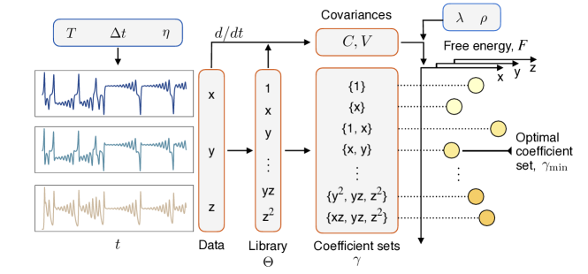
Figure 1: Schematic representation of the questions Z-SINDy aims to answer. A dataset consists of a trajectory of time length $T$ sampled with time step $\Delta t$ and measurement noise of magnitude $\eta$ (left blue box). From the data, a library of nonlinear functions $\Theta_{i}(\vec{x})$ is computer. The library functions are combined with empirical derivatives of the trajectory to compute the covariance matrices $C$ and vectors $\vec{V}$. The covariances along with the algorithm hyperparameters of sparsity $\lambda$ and resolution $\rho$ (right blue box) are used to compute the free energies $F^{(}l)_{\gamma_{l}}$ that quantify the balance between goodness of fit and number of fitting solutions. The best fit coefficient set $\gamma_{min}$ is the one that corresponds to the lowest free energy. In this paper we study how the probability of choosing the correct coefficient set depends on the parameters in blue boxes.

II.1 Background

System identification begins with an observed trajectory $\vec{x}(t)$ of a $d$-dimensional dynamical system. The trajectory covers the length of time $T$ sampled with period $\Delta t$, resulting in $n=T/\Delta t$ data points. For synthetic trajectory data, we presume that the integration time step is much smaller than $\Delta t$, making the integration error negligible. Trajectory measurement incurs uncorrelated additive Gaussian noise of magnitude $\eta$ in each dimension of dynamics. From the trajectory we compute the empirical derivative $\dot{\vec{x}}$ with second-order centered finite difference method to simplify the interpretation.

The goal of sparse equation discovery is to extract a dynamical equation $\dot{\vec{x}}=f(\vec{x})$ from the observed trajectories of $\vec{x}$, where $f(\cdot)$ is a sparse analytical expression. When $f(\cdot)$ is given by a library of candidate nonlinear functions, we seek an equation of the form:

$$\dot{x_{l}}\approx\sum\limits_{i=1}^{N}\Theta_{i}(\vec{x})^{T}\Xi_{il},$$ (1)

where the index $l$ enumerates the dynamical variables, the left hand side is the empirical derivative and right hand side is a linear combination of $N$ nonlinear functions of dynamical variables $\Theta_{i}(\vec{x})$ (i.e. the library) with a matrix of coefficients $\Xi_{il}$. The Sparse Identification of Nonlinear Dynamics (SINDy) seeks to optimize for the sparsest matrix of coefficients $\Xi_{il}$ that minimizes the residual of (1). This optimization problem involving two competing objectives - sparsity and fitness - leads to a challenging non-uniqueness in the resulting models. In practice, the problem is typically solved by optimizing a loss function that combines linear regression with a sparsity penalty. While sparsity is directly measured by the $\norm{\Xi}_{0}$ pseudonorm on the model coefficients, it is usually approximated by either the $\norm{\Xi}_{1}$ norm or sequential thresholded least squares [35, 7].

Where optimization-based SINDy provides a point estimate of the coefficients, Bayesian approaches aim to extract the maximum amount of information from the data, while providing an uncertainty quantification of the resulting equation. In the Bayesian setting, sparsity can be promoted by the choice of a sparsifying prior, such as Laplace, spike-and-slab, or horseshoe [36, 31, 33]. These priors aim to concentrate the posterior probability near $\Xi_{il}=0$, while remaining differentiable to enable Monte Carlo sampling.

The interplay of sparsity with large numbers of variables and data points in a probabilistic setting attracted significant attention of the statistical mechanics community, particularly the theory of disordered systems [28]. By using the so-called replica trick, researchers averaged over random data matrices to obtain the average behavior of different classes of inference problems, revealing multiple detectability and algorithmic phase transitions [24, 26, 27, 37]. Our approach here is different in two key aspects: first, we focus on identifying not a finite fraction of relevant variables but a finite number, thus attaching more interpretation to each term; second, instead of averaging over generic random Gaussian data matrices, we work with trajectory data, including the sampling period and numerical differentiation effects.

II.2 Z-SINDy

In the present paper we separate the Bayesian inference problem into two layers: the discrete layer describes which coefficients are active (non-zero), while the continuous layer describes the values of active coefficients. In particular, this new setting does not require the prior to be differentiable, allowing us to use a much simpler Bernoulli-Gaussian functional form:

$$p(\Xi)= \prod_{i}\frac{1}{1+e^{-\Lambda}}(\delta(\Xi_{i})+w(\Xi_{i})e^{-\Lambda})$$ (2)

$$= \frac{1}{(1+e^{-\Lambda})^{N}}\sum\limits_{\gamma}\left(\prod\limits_{i\notin\gamma}\delta(\Xi_{i})\right)\left(\prod\limits_{i\in\gamma}w(\Xi_{i})\right)e^{-\Lambda\absolutevalue{\gamma}},$$ (3)

where we omitted the index $l$ for simplicity of notation, since the inference is independent in each dimension with a shared set of library terms $\Theta_{i}(\vec{x})$. Within the Bernoulli-Gaussian prior, the hyperparameter $\Lambda$ regulates sparsity; $\delta(\cdot)$ is Dirac delta function that can be thought of as an infinitely narrow Gaussian; and $w(\cdot)$ is a prior function that quantifies the parameter uncertainty in the absence of data, which we take to be in the limit of an infinitely wide Gaussian (see SI for additional discussion). The prior form of (2) is symmetric under the permutation of indices $i$, highlighting that the inference procedure does not have a preference of any variable combination before seeing any data. The symmetry is made even more explicit by multiplying out the brackets to get to (3), which is given as a sum over the coefficient sets, e.g. $\gamma=\varnothing,\{\text{x,yz}\},\{\text{1,y,z,xy,xz}\}$. For $N$ library terms there are $2^{N}$ possible discrete coefficient sets that form the power set of library indices $\{\gamma_{l}\}=\raisebox{1.79993pt}{\Large$\wp$}(\{i\})$. The prior probability of any coefficient set depends only on its size $\absolutevalue{\gamma}$ but not its identity, and increasing the value of $\Lambda$ shifts progressively more probability weight from larger to smaller sets, while maintaining unbroken symmetry under index permutation.

Along with the prior, we define the forward model, i.e. the probability of observing the data given the coefficients (likelihood):

$$p(x|\Xi)\propto\exp(-\frac{1}{2\rho^{2}}\sum\limits_{t}\left(\dot{x}-\vec{\Theta}^{T}\vec{\Xi}\right)),$$ (4)

where we suppressed the time indexing on the empirical derivative and the library terms. The resolution hyperparameter $\rho$ regulates how closely the nonlinear function library aims to approximate the empirical dynamics derivative.

We use the forward model and the prior we derive the posterior via Bayes rule:

$$p(\Xi|x)=\frac{1}{\mathcal{Z}}\exp(-\frac{1}{2\rho^{2}}\sum\limits_{t}\left(\dot{x}-\vec{\Theta}^{T}\vec{\Xi}_{l}\right)-\Lambda\norm{\vec{\Xi}}_{0}),$$ (5)

where the expression inside $\exp(\cdot)$ is the $l_{0}$ regularized SINDy functional [7]. In statistical mechanics, this would be akin to Boltzmann’s distribution with $\rho^{2}$ playing the role of temperature, $\Lambda$ playing the role of chemical potential (cost of adding new particles to the system), and $\mathcal{Z}$ the partition function (normalization) of the distribution. The mode of this distribution, or the Maximum A Posteriori (MAP) estimate of the coefficients, would be equivalent to the original SINDy problem statement, but the $l_{0}$ regularization is challenging to optimize in practice.

Instead of performing optimization, we disentangle the mixture of continuous and discrete degrees of freedom in (5) by using the factorized form of the prior (3) to rewrite the posterior into a hierarchical form as a choice of active coefficient set followed by a choice of coefficient values. In this factorized form the posterior takes form of a linear mixture of multivariate Gaussians:

$$p(\Xi|x)= \frac{\sum_{\gamma}p(\vec{\Xi}_{\gamma}|\gamma,x)\mathcal{Z}_{\gamma}}{\sum_{\gamma}\mathcal{Z}_{\gamma}}$$ (6)

$$\mathcal{Z}_{\gamma}\equiv e^{-F_{\gamma}}=e^{-F^{\prime}_{\gamma}}e^{-\Lambda\absolutevalue{\gamma}}$$ (7)

$$F^{\prime}_{\gamma}= -\ln\mathcal{Z}_{0}-\frac{|\gamma|}{2}\ln(2\pi\rho^{2})+\frac{1}{2}\ln\det C_{\gamma}$$

$$- \frac{1}{2\rho^{2}}\vec{V}^{T}_{l,\gamma}C^{-1}_{\gamma}\vec{V}_{l,\gamma_{l}}$$ (8)

$$F_{\gamma}\equiv F^{\prime}_{\gamma}+\Lambda\absolutevalue{\gamma}=F^{\prime}_{\gamma}+\lambda\cdot n\absolutevalue{\gamma},$$ (9)

where the statistical weights $\mathcal{Z}_{\gamma}$ quantify the relative importance of each coefficient set (evidence) and are thus the central objects of the method, inspiring the name Z-SINDy. Since the statistical weights vary over many orders of magnitude, it is more convenient to represent them on logarithmic scale as free energies $F_{\gamma}$. In Bayesian terminology, $\mathcal{Z}_{\gamma}$ is the likelihood of each coefficient set, and $F_{\gamma}$ is the negative log-likelihood. The free energy is computed directly from subsets of the precomputed empirical correlation matrix $C$ and vectors $\vec{V}_{l}$ of library functions with each other and with empirical derivatives (see SI for derivation).

Much like in statistical physics the free energy quantifies the balance of energy and entropy of a coarse-grained state[38], here the free energy represents the goodness of fit of the empirical derivatives $\dot{x}_{l}$ with respect to all possible continuous values of coefficients within the same active set. The derivation and the final functional form of (8) are closely similar to the Bayesian Information Criterion (BIC) that combines the likelihood of a model with a penalty based on the number of parameters [39]. The free energy expression (9) selects for sparse solutions in two ways: while the BIC-like penalty we term “natural sparsity” scales with $\ln n$ (see SI for derivation), the prior driven penalty scales as $\Lambda=\lambda\cdot n$. The following sections use the free energy computation to compute the full posterior and its marginals to analyze model inference in different regimes.

III Results

III.1 Free energy trends

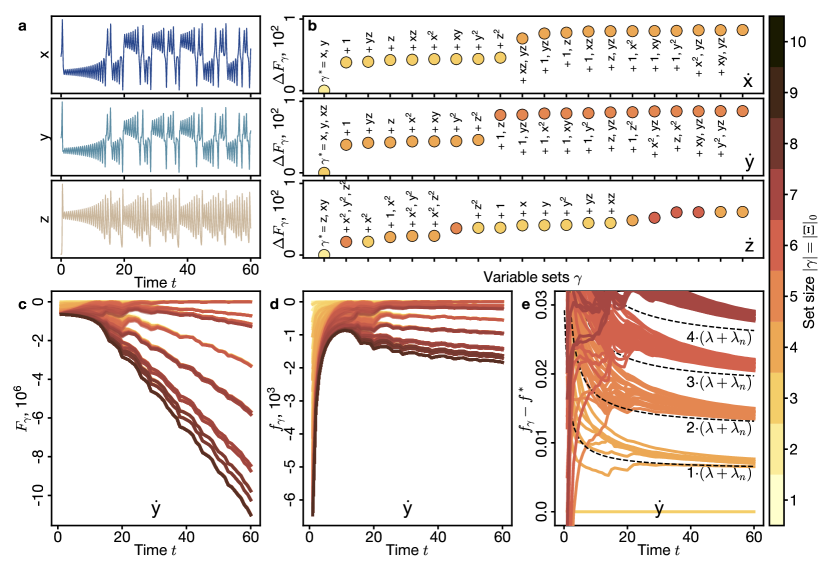
Figure 2: Free energy trends in Z-SINDy inference. (a) Sample trajectories of the Lorenz attractor sampled with time sampling period of $\Delta t=0.01$ and no noise. (b) Free energies of different coefficient sets for each dimension of dynamics relative to the best fit set $\gamma^{*}$ computed at $\rho=1.0$. Other coefficient sets are labeled by the extra library terms with respect to $\gamma^{*}$. (c) Free energy $F_{\gamma}$ of each of the $2^{N}=1024$ coefficient sets over time. (d) Free energy per data point $f_{\gamma}$ of each coefficient set. (e) Relative free energy per data point $f_{\gamma}-f^{*}$ of each coefficient set, stratified by the sparsity penalty $\lambda=0.006$ and the natural sparsity penalty $\lambda_{n}$. The color of markers and curves corresponds to the number of coefficients in each set $|\gamma|$.

In order to establish intuition for free energy scaling, we use the expression (8) to compute the free energies of all variable sets for an example model. We choose to focus our in-depth analysis on one 3-dimensional chaotic dynamical system, the classic Lorenz attractor first integrated numerically by Ellen Fetter [41, 42] (Fig. 2a), since it is a fairly typical chaotic system with polynomial nonlinearity [43], and the performance of SINDy-family algorithms does not strongly correlate with different features of chaotic systems [44]. For the library terms, we consider all monomials in variables $x,y,z$ up to 2nd order, resulting in $N=10$ library terms and $2^{N}=1024$ possible coefficient sets. The computational infrastructure of evaluating the library terms is based on the PySINDy package [45].

For a constant and moderate trajectory length $T$ and sparsity penalty $\lambda$ the free energies of different variable sets form a hierarchy shown in Fig. 2b for each dimension of dynamics: the correct variable set $\gamma^{*}$ has the lowest free energy, while the next several sets with higher free energies all have extra terms. If the trajectory data is only considered up to a variable upper limit of time $t$, the free energies of each variable set have asymptotically linear trajectories of different slopes (Fig. 2c). In order to compare the slopes, we compute the intensive free energy per data point $f_{\gamma}=F_{\gamma}/n$ that is asymptotically constant for each variable set (Fig. 2d). We further disentangle the different sets by computing the intensive free energy relative to its lowest value $\Delta f_{\gamma}=f_{\gamma}-f^{*}$ (Fig. 2e). By construction the relative free energy of the correct variable set is zero, and free energies of other sets are asymptotically stratified by the constant intensive sparsity penalty $\lambda$. While the sparsity penalty is an externally chosen hyperparameter of Z-SINDy, at low sample sizes the Bayesian inference procedure itself introduces an additional “natural” sparsity $\lambda_{n}=\ln(n/2\pi\rho^{2})/2n$ that enhances the selection for sparse coefficient sets similar to the BIC (see SI for derivation).

The asymptotically constant free energy per data point in this inference problem is similar to the thermodynamic free energy of interacting particle systems. For particle systems, nonlinear scaling of free energy with system size usually implies either long-range particle interactions or strong boundary effects. Indeed, the inference free energy has a nonlinear scaling at early times ($t<10$ on Fig. 2c), when the Lorenz dynamical system has only explored one lobe of the attractor and has not yet demonstrated the switching behavior. At longer times, the chaotic dynamics forget the initial condition and the effective sample size scales linearly with the amount of data, leading to a condensation of inference, as we explore in the following section.

III.2 Inference condensation

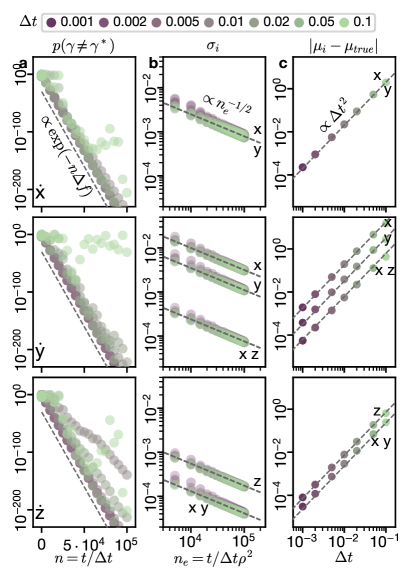
Figure 3: Condensation of Z-SINDy inference for trajectory datasets of variable runtime $t$, sampling time period $\Delta t$, resolution parameter $\rho\in\{0.1,1.0,10\}$. (a) The probability of choosing any variable set other than the one with lowest free energy decays exponentially with trajectory length. (b) The posterior standard deviation of each inferred coefficient decays as inverse square root of the trajectory length. (c) The absolute error of the posterior mean coefficient is limited by the systematic error of the finite difference derivative of the trajectory. Trend lines guide the eye to illustrate the functional form of the scalings. The line labels in (b-c) indicate which coefficient the standard deviation and the mean correspond to. Rows correspond to the three dimensions of dynamics. The standard deviation and error of the mean for the two variables explaining $\dot{x}$ coincide.

In order to connect the scaling of free energy to the outcomes of the inference procedure, we consider the limiting case of the posterior distribution (6). The probability of selecting the lowest free energy set is driven by the free energy gap between it and the next set:

$$p(\gamma^{*})=\frac{1}{1+\sum\limits_{\gamma\neq\gamma^{*}}e^{-(F_{\gamma}-F_{\gamma^{*}})}}\approx 1-e^{-n\Delta f},$$ (10)

where $\Delta f$ is the asymptotic difference of free energy per data point between the best and the second-best fitting coefficient sets. This expression implies that the probability of selecting any other variable set decays exponentially with trajectory length across a wide range of sampling frequencies (Fig. 3a). While the statistical weights $\mathcal{Z_{\gamma}}$ can get exponentially large or small, risking numerical overflow or underflow problems, the values of free energies do not face that problem. The exponential suppression of sub-optimal coefficient sets implies that it is sufficient to look for the lowest free energy coefficient set at given dataset parameters and inference hyperparameters.

Given the condensation of the discrete part of inference, what happens to the continuous part? Per (6), the Gaussian mixture reduces to a single multivariate Gaussian distribution with the covariance and mean parameters driven by the empirical correlations $C_{\gamma^{*}}$ and $\vec{V}_{l,\gamma^{*}}$. The posterior covariance matrix is given by $\Sigma_{\gamma^{*}}=\rho^{2}C^{-1}_{\gamma^{*}}$, scaling with the resolution parameter $\rho$ but decaying with increasing trajectory length, which can be combined into an effective time scale $n_{e}=t/\Delta t\rho^{2}$. The standard deviations of the posterior along each coefficient direction have different magnitudes but identical scaling of $n_{e}^{-1/2}$ as in the Central Limit Theorem (Fig. 3b).

The posterior Gaussian mean is given by $\vec{\mu}=C^{-1}_{\gamma}\vec{V}_{l,\gamma}$, which quickly converges to a constant value, which is not necessarily equal to the ground truth $\vec{\mu}_{true}$. Since the linear regression against the nonlinear library terms aims to explain the empirical derivative, it inherits the systematic error of the numerical differentiation procedure, well known in the studies of numerical integration [46] but rarely highlighted in system identification. For the second-order finite difference derivative employed here the systematic error scales as $\order{\Delta t^{2}}$, and this scaling propagates to the error of the mean (Fig. 3c). For large enough trajectory length the standard deviation becomes smaller than error of the mean $\sigma_{i}<\absolutevalue{\mu_{i}-\mu_{true}}$, and thus the inference converges to a small region that does not include the ground truth values.

Increasing the trajectory length leads to a condensation of inference to a particular set of coefficients with a narrow range of values. However, if the amount of data asymptotically does not distinguish between inferred models, then what does? In thermodynamic systems, free energy per particle is typically a function of external thermodynamic variables, such as temperature, magnetic field, or chemical potential. Small changes of the external parameter can shift the global free energy to a different state, leading to a thermodynamic phase transition. In a similar way, small changes in the inference hyperparameter $\lambda$ or noise in the data $\eta$ can lead to abrupt changes in the inferred model, as we show in the following sections.

III.3 Sparsity transitions

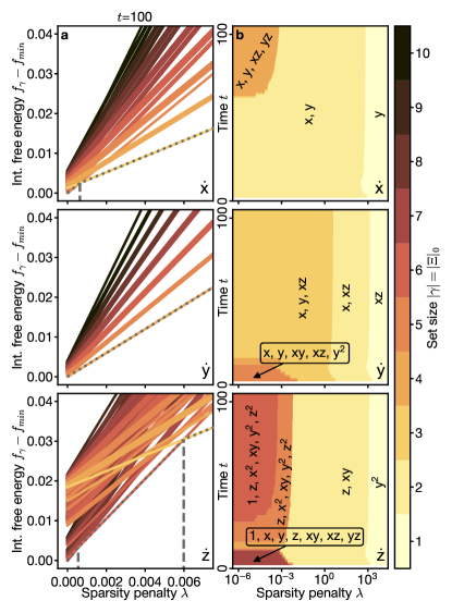
Figure 4: Sparsity penalty selects sparse solutions. (a) For a fixed trajectory of length $t=100$, the penalized intensive free energies of each coefficient set are linear functions of the sparsity penalty $\lambda$ with the slope given by the number of terms and the intercept by the goodness of fit. At any value of $\lambda$, the posterior condenses on the lowest free energy set (piecewise linear dotted lines), switching abruptly between solutions of different sparsity (vertical dashed lines). (b) As the sparsity penalty varies over many orders of magnitude, the best fit coefficient set changes abruptly several times from large to sparse, with a finite range of $\lambda$ recovering the correct set. The color of lines and backgrounds corresponds to the number of coefficient in each set.

The goal of SINDy-family approaches is to balance the data fit with the parsimony of the inferred models, operationalized by sparsity. Instead of prescribing a particular number of equation terms, the algorithm is supposed to find it adaptively, but how exactly does the sparsity penalty parameter $\lambda$ lead to sparse solutions?

We have established in the previous section that with enough data, Z-SINDy would always select the model with lowest free energy. Given a constant dataset, the penalized free energies are linear functions of the penalty ((9)), with the intercept given by data fit at zero penalty, and the slope given by the number of terms. Graphically, the ensemble of all the linear functions looks like a fan plot with all-integer slopes $1,2,3,\dots$ (Fig. 4a). As the external sparsity penalty $\lambda$ increases, the lowest free energy line changes in a series of abrupt transitions from lower-intercept higher-slope to higher-intercept lower-slope (shown in vertical dashed lines), similar to the plots produced by Least Angle Regression (LARS) [47]. However, because of the natural sparsity effect, the inference selects for sparse solutions even at $\lambda=0$. In order to include both external and natural sparsity, we therefore vary both $\lambda$ and the trajectory length $t$.

At moderate to high sparsity penalty $\lambda$ the selected variable sets are practically independent of trajectory length (Fig. 4b), but at low $\lambda$ the selection changes in two ways. Very short trajectories do not explore the entirety of available phase space: for the Lorenz system, the trajectory stays within a single lobe of the attractor for $t<15$ (Fig. 2a), and thus Z-SINDy identifies less sparse models (bottom-left corner of Fig. 4b panels). For moderate trajectory length the correct coefficient set is recovered for a wide range of $\lambda$ because of the natural sparsity $\lambda_{n}$. For long trajectories the natural sparsity disappears, leading to identification of less sparse sets (top-left corner of Fig. 4b panels). We conclude that Z-SINDy correctly identifies the sparse set of coefficients within a window of several orders of magnitude of sparsity penalty $\lambda$, but the boundaries of the region are quite abrupt.

III.4 Noise transition

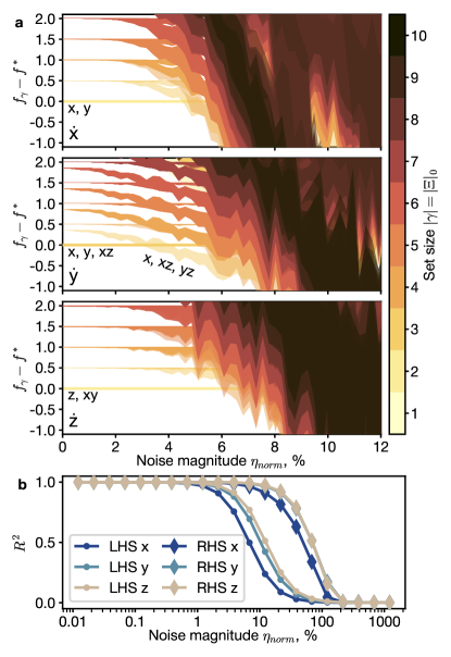
Figure 5: Additive noise prevents the identification of the correct coefficient set. (a) Each panel shows the free energies per data point with respect to the correct set for a trajectory of length $t=60$ at sampling period $\Delta t=0.01$. For each coefficient set, the shaded region shows the range of free energies across 10 realizations of random noise of given relative magnitude $\eta/\bar{\sigma}_{data}$, stratified by sparsity penalty $\lambda=0.5$. The color of the shaded regions corresponds to the number of coefficients in each set. (b) Coefficient of determination $R^{2}$ of the noisy left and right hand sides of the equation of motion with the correct right hand side for each dimension of dynamics, averaged over 5 noise realizations.

Along with sparsity, another important limitation to the performance of SINDy algorithms is the noise in the data. The robustness of SINDy is usually measured by how fast the error in the inferred coefficients grows with noise magnitude, and thus how much noise can the inference tolerate. While the denoising approaches [48, 49] and the weak form SINDy [10] improve noise tolerance significantly, they do not explain how the noise-induced breakdown happens, whether collecting a longer trajectory helps, and why denoising improves performance so much.

We seek to explain the noise-induced breakdown in free energy terms. The free energy of any variable set $\gamma$ depends not only on the trajectory length $t$, sparsity penalty $\lambda$, and noise magnitude $\eta$, but also on the noise realization. Within each realization, we compute the deterministic free energy per data point relative to the correct set $\gamma^{*}$ in each dimension, and then collect free energy statistics across multiple noise realizations. The relevant free energy statistic is not its mean but its range of fluctuations, since the inference condenses to the coefficient set with the lowest free energy.

The noise-induced transition graphically looks like an overlap between the horizontal line of the correct set and the free energy range of one of the competing sets (shaded regions in Fig. 5a). We normalize the noise magnitude by the standard deviation of the original trajectory averaged across the dimensions $\eta_{norm}=\eta/\sigma_{data}$. At low noise magnitude $\eta_{norm}$, the correct coefficient set $\gamma^{*}_{l}$ has the lowest free energy, clearly stratified from all other ones by the sparsity penalty, and is thus selected in inference. As noise magnitude increases, at about $\eta_{norm}\approx 4\%$ the model for $\dot{y}$ changes as the set $\gamma^{*}=\{\textrm{x, y, xz}\}$ first overlaps with the range of free energies of $\gamma=\{\textrm{x, xz, yz}\}$ and then lies entirely above the range. Within the free energy range overlap, the inference condenses to a single coefficient set that depends on the realization of the random noise, and thus the inference is unstable. At higher levels of noise above $\eta_{norm}\approx 6\%$ the horizontal line of the correct set lies fully above multiple overlapping free energy ranges, and thus the inference procedure would confidently select a coefficient set from many possible alternatives, none of which are correct. This inference scenario is qualitatively similar to the detection of weak communities in complex networks, where the single eigenvalue that carries community information gets buried within a continuous band of random eigenvalues [25].

Can this inference collapse be avoided with larger amounts of data? As trajectory length $t$ increases, the width of the free energy range shrinks proportional to $t^{-1/2}$, thus reducing the range of noise magnitudes $\eta$ where the inference outcome is realization-dependent (see SI for discussion). However, since the mean free energy per data point converges to a constant $\eta$-dependent value, the takeover of the correct coefficient set $\gamma^{*}$ by one or more competing ones is inevitable.

What part of the data processing pipeline drives the inference collapse? SINDy approaches aim to balance the noisy versions of the left and right hand sides of (1) $LHS_{noisy}$ and $RHS_{noisy}$ (LHS is derivatives, RHS is library terms) approximately, but how good is that approximation? We can perform that comparison since for a synthetic dataset we have access to both clean and noisy trajectories. The clean trajectory is an exact solution to (1) up to integration error, for which the two sides of the equation match $LHS_{true}=RHS_{true}$ and can be computed exactly by using the ground truth coefficients $\Xi_{il,true}$. We thus have three time series for each dimension, the linear correlation between which is easily measured by the coefficient of determination $R^{2}$.

The $R^{2}$ smoothly decrease from 1 at low noise to 0 at high noise, where neither LHS nor RHS of the noisy equation carry any resemblance to the truth (Fig. 5b). While there is a slight variation of the decay point of curves between dimensions, LHS decays at almost an order of magnitude lower noise level, and is thus primarily responsible for SINDy breakdown. Since the core of SINDy is linear regression, the curves such as Fig. 5b can be plotted for any denoising numerical derivative method and sampling time period and used as a diagnostic method to identify the limiting factor of performance and thus the most promising algorithmic improvement.

III.5 Uncertainty Quantification

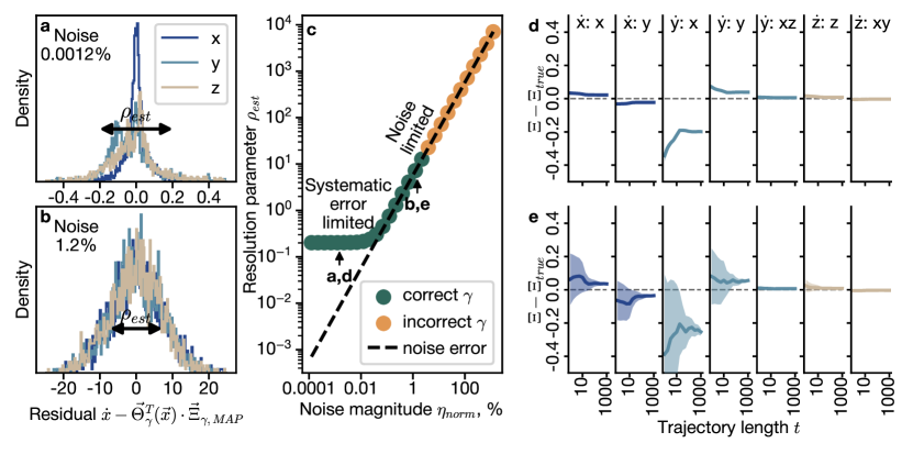
Figure 6: Uncertainty quantification from empirical residual. (a-b) Histograms of the derivative residual across the length of the trajectory for each of three dimensions of dynamics. The black arrow indicates the $\pm 1\cdot\rho_{est}$ range, equal to the sample standard deviation of the residual. (c) Inferred resolution parameter $\rho_{est}$ at each noise level. The marker color indicates whether the correct set of coefficients has been identified at given noise level. At low noise the residual is limited by the systematic error and thus the resolution parameter is constant. The dashed line indicates the analytic prediction of noise driven error in the derivative, which dominates at high noise. (d-e) Marginal posterior distributions for each of the seven active terms in the Lorenz system. The solid curves show the posterior mean relative to ground truth, the shaded region indicates $\pm 1$ standard deviation. The horizontal axes cover the range of trajectory length $t\in[1,1000]$ on logarithmic scale. Panels (a,d) are computed at low noise, panels (b,e) at moderate noise.

The analysis of the noisy LHS and RHS leads to the uncertainty quantification of the inferred coefficients in the limit of low data. The posterior distributions of all coefficients are Gaussian with parameters derived from the correlations $C,\vec{V}_{l}$, but require knowing the resolution parameter $\rho$. The resolution parameter describes the distribution of the the residual between the noisy LHS and RHS of the dynamical equation, and can be estimated from the empirical distribution by using the Maximum A Posteriori (MAP) values of the coefficients $\vec{\mu}$:

$$\rho_{est}=\sqrt{\frac{1}{n\cdot d}\sum\limits_{t,l}\left(LHS_{l,noisy}-RHS_{l,noisy}\right)^{2}}.$$ (11)

While for each dimension the residual itself $LHS_{noisy}-RHS_{noisy}$ is expected to have a Gaussian distribution, we can check the shape of the distribution empirically (Fig. 6a-b). At low noise level the distribution is different for each dimension and has a complex multimodal shape with long tails (panel a), while at moderate noise the distributions for all three dimensions have a consistent Gaussian shape (panel b). As the amount of noise on the trajectory varies over several orders of magnitude, the estimated resolution parameter $\rho_{est}$ switches from a flat value driven by the systematic error of the finite sampling period to the noise driven value $\rho=\eta/\Delta t\sqrt{2}$ (Fig. 6c, see SI for derivation).

The resolution parameter is the last missing piece in computing the error bar on the inferred coefficients and comparing them to the ground truth. At low noise the error bar is incredibly small, so that the systematic error in the coefficients is immediately visible for all trajectory lengths (Fig. 6d). At moderate noise the error bar increases and overlaps with the ground truth so that the systematic error is not visible at short trajectory length. As the trajectory length increases, the error bar shrinks proportional to $t^{-1/2}$ as discussed before, resulting in the same value of the statistically significant systematic error.

III.6 Inference phase diagram

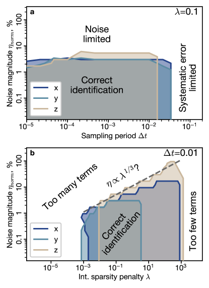
Figure 7: Inference of the correct dynamical equations is limited by the data noise $\eta$, sampling period $\Delta t$, and sparsity penalty $\lambda$. (a) Inference fails when either the noise level crosses a threshold (noise limited), or the sampling period becomes too large to resolve the smallest time scale of the dynamical system (systematic error limited), with the boundaries consistent across the three dimensions of dynamics. (b) The region of correct inference in noise and sparsity parameters is limited on three sides: too few terms at high $\lambda$, and too many terms at low $\lambda$ or high $\eta$. The dashed line guides the eye to illustrate a speculative power law on critical noise level $\eta\propto\lambda^{1/3}$.

Having characterized the inference breakdown with sparsity and noise separately, we can now answer the questions about the joint effect of dataset parameters and inference hyperparameters on the viability of system identification. We have shown that inference rapidly condenses to a single coefficient set with growing trajectory length $t$ that is determined by the lowest free energy per data point. Moderate values of $t$ incur the natural sparsity effect, but it vanishes for $t\to\infty$, so that the selected coefficient set becomes independent of data quantity. The value of the resolution hyperparameter $\rho$ modulates the inference condensation and affects the size of the confidence interval for the coefficients. This value can be chosen to match the statistics of the residual $\dot{x}_{l}-\vec{\Theta}^{T}\cdot\vec{\Xi}_{l}$ and provide accurate uncertainty quantification.

The remaining parameters interact in a more complex way as shown in the phase diagrams of Fig. 7. The noise magnitude $\eta_{norm}$ and sampling period $\Delta t$ impose separate, orthogonal limitations (Fig. 7a). At large sampling period, the samples can no longer resolve the smallest time scales of system dynamics and result in a large systematic error in the empirical derivative. At the same time, a small sampling period combined with presence of noise results in a large statistical error in the empirical derivative. However, while the error of each derivative sample grows as $1/\Delta t$, the number of samples per unit time grows at precisely the same rate $1/\Delta t$ and the two effects almost cancel each other out, resulting in a nearly horizontal upper bound of correct identification (see SI for additional discussion).

The interaction of noise magnitude $\eta_{norm}$ with sparsity penalty $\lambda$ is even more complex (Fig. 7b). The noiseless regime of identification has been explored in Fig. 4, revealing a finite range of several orders in $\lambda$ where the identified coefficient set has not too many and not too few terms, with a narrower range for $\dot{y}$ that has more terms in the correct coefficient set. While the sparsity penalty creates a gap between the free energies of sets of different size, growing noise level gradually reduces this gap until a free energy crossover (Fig. 5a). Qualitatively, a larger initial gap $\lambda$ would require more noise $\eta$ to close, resulting in a positive slope of the limiting curve on the phase diagram. The trade-off has the approximate shape of a power law $\eta\propto\lambda^{1/3}$ across six orders of magnitude of $\lambda$, but the limited resolution of the phase diagram and the complexity of the free energy landscape prevent a simple explanation of this scaling, leaving an important opening for further work.

IV Discussion

In this paper we introduce Z-SINDy, a Bayesian version of a simple form of SINDy that we analyze through the prism of statistical mechanics to understand how it works—and, importantly, how it breaks. We explicitly separate the discrete and continuous parts of equation coefficient inference and derive a closed-form posterior probability distribution of the coefficients. The probability of a particular discrete set condenses exponentially with growing trajectory length to a single coefficient set, though the set is not guaranteed to be correct. Even if the identified library terms are qualitatively correct, the value of the coefficients is subject to both systematic and noise driven errors. A combination of natural and externally imposed sparsity penalties induce a set of discontinuous transitions from a large coefficient set to a sparse one. The inference procedure correctly identifies the sparse set when the trajectory has moderate noise but fails at large noise, where the inferred equation depends strongly not only on noise magnitude, but also its specific realization. Before the noise induced transition, matching the residual statistics provides UQ for the inferred model. The combination of these results establishes the boundaries of applicability of SINDy, and the warning mechanisms for its breakdown.

Our study is not unique in application of Bayesian inference to the SINDy framework. While previous recent work relied on costly Monte Carlo sampling from the posterior [31, 33], several studies conducted concurrently but independently from ours used the closed-form computation of model evidence [50, 51]. They show that using Bayesian inference with Gaussian priors gives rise to the effect we term “natural sparsity”, but do not consider an explicitly sparsity-promoting prior such as Bernoulli-Gaussian. As a result, they focus on the $L_{1}$ error of the determined coefficients rather than the $L_{0}$ error in identifying the correct coefficient set $\gamma$. We provide both the boundaries of correct system identification, as well as the asymptotic scaling of coefficient errors with dataset size and sampling period.

IV.1 Statistical mechanics analogies

Instead of searching for the best fit alone, we characterize the whole landscape of models on a logarithmic scale by computing their free energies. This computation integrates out the continuous coefficient values and focuses on the coefficient sets, building a connection with coarse-grained statistical mechanics and thermodynamics of interacting particle systems [38]. The consideration of long time trajectories is akin to the thermodynamic limit and motivates the evaluation of intensive free energy per data point similar to the free energy per particle. The thermodynamic cost of adding another “particle” type into the model, i.e. another SINDy term, is given by the sparsity penalty $\lambda$ that functions as (negative) chemical potential. The chemical potential of all “particles” is identical, but the interactions between them are driven by the trajectory data and thus select a particular “particle” set, i.e. a set of active SINDy library terms. As the parameters of the dataset or the hyperparameters of the inference procedure are adjusted, the inferred model can change discontinuously, akin to a phase transition or a dynamical system bifurcation. The pattern of free energies of different coefficient sets exhibits rich structure, opening avenues for further study, including connection to the entropy metrics of dynamical system trajectories [52].

The connections between statistical mechanics, statistical inference, and machine learning have a rich history, focusing primarily on the average-case behavior of prediction risk [23]. Statistical mechanics helped identify and describe multiple inference regimes and phase transitions between them, from network structure inference to constraint satisfaction to compressed sensing [24, 25, 26, 28]. The so-called replica method has been used to characterize the regularized least squares regression that also lies at the core of SINDy [37], identifying the regimes where local greedy algorithms can efficiently identify the optimal set of predictor variables [27]. However, statistical physics studies often consider the large-data case $n\to\infty$ in which, in our notation, $\absolutevalue{\gamma}/n=const$, i.e. the set of selected coefficients is sparse but growing. This paper enriches the discussion by analyzing the case of dynamical systems in which the number of differential equation terms staying constant regardless of trajectory length $\absolutevalue{\gamma}=const$, paying attention to the specific interpretable nature of individual terms, and painting a detailed picture of inference breakdown.

IV.2 Integration with other SINDy techniques

The system identification scenario considered here aims to extract a parsimonious model [21], but focuses only on one aspect of parsimony—sparsity—over other aspects such as discovery of coordinates and parametric dependencies, both of which have been included in other data-driven methods. The coordinate discovery has been addressed by combining dynamics discovery with an autoencoder neural network that automatically discovers the sparse coordinates either in the optimization framework [53, 54] or the Bayesian framework [33]. The parametric dependence can be inferred by including a parameter library along with the dynamical equation library [55]. The parsimony requirements can be supplemented by other desired features of dynamical systems such as global stability [56]. Integrating fast posterior computations from the present paper with nonlinear coordinate transformation discovery, parametric inference, and dynamic stability remain important avenues for further work. Within the analysis of trajectories, additional improvements can be achieved by a finer-scale analysis of free energy fluctuations with respect to the general trend $F\sim f\cdot n$, as well as active learning to proactively sample the unexplored parts of phase space akin to the technique suggested in Refs. [30, 51].

All SINDy approaches rely on regression and thus require a reliable estimation of the dependent variable, the trajectory derivative. While here we employ the simplest derivative method, finite difference, most other contemporary SINDy algorithms rely on some version of denoising derivative, such as total variation [57], spectral derivative [58], weak form [10], or basis expansion [32, 11], which drastically improve the benchmark noise tolerance. However, such performance improvement might be misleading in quantifying the parameter uncertainty since the data uncertainty is discarded [32]. Moreover, the denoising process is itself parametric and trades random noise for a systematic error in the derivative and the library terms [57, 46], requiring hyperparameter optimization [22, 59]. For an experimental system where the ground truth equations are unknown, it is thus unclear whether small variations of the dynamical variables are due to measurement noise or genuine fine-scale dynamics. Z-SINDy does not make a choice between those options by keeping $\rho$ as a free parameter of how closely the linear combination of library terms should approximate the derivative. Since both the derivative and the library terms suffer from noise contamination, it is challenging to pick $\rho$ a priori but it can be estimated after the SINDy fit from the remaining unexplained variance in the derivative $\dot{x}-\Theta^{T}\cdot\Xi$ (see SI for additional discussion).

The free energy analysis presented here makes a prediction of the identification phase diagram for a known ground truth dynamical model. On one side, the residual distribution (Fig. 6a-b), the phase diagrams (Fig. 7), and the $R^{2}$ plots (Fig. 5b) are powerful diagnostic tools that quantify the limits of performance of a particular numerical algorithm and thus suggest how the boundary of detectability can be pushed, with the most immediate gains available through denoising. On the other side, the analysis establishes the noise tolerance that can be part of a closed-loop inference system: for a given dataset one can fit and integrate a SINDy model, compute its noise tolerance, and estimate the empirical noise magnitude. If the empirical noise is above the tolerance, then the model is misleading and should be rejected.

IV.3 Computational considerations

The main computational advantage of Z-SINDy is the closed form evaluation of the posterior distribution, avoiding the costly techniques of bootstrap resampling [30], Markov Chain Monte Carlo [33], and repeated ODE integration [31] that are required in other UQ system identification methods. On the other side, an important computational limitation to our method is the combinatorial enumeration of coefficient sets. While the free energy (8) of any particular set $\gamma$ is very cheap to compute, the number of all possible sets grows exponentially with the number of library terms $\absolutevalue{\{\gamma\}}=2^{N}$. In this paper we chose to evaluate free energies exhaustively for all sets to illustrate their scaling behavior. At the same time, the free energies of different sets are heavily stratified (e.g. Fig. 2c), and only a small fraction of sets are involved in sparsity- or noise-induced breakdowns. In order to make Z-SINDy more computationally efficient and thus tractable for realistic systems, future work should aim to understand the patterns of free energies better to reduce the number of sets to evaluate, for instance by using greedy methods [51], subset selection [60], least angle regression [47], mixed-integer optimization [29], or branch-and-bound methods [61]. At the same time, we hope that the physical intuition of coarse-graining, chemical potentials, and free energies per data point would inform the further development of statistical methods for dynamical systems.

References

- Ljung [2010] L. Ljung, Perspectives on system identification, Annual Reviews in Control 34, 1 (2010).
- North et al. [2023] J. S. North, C. K. Wikle, and E. M. Schliep, A review of data-driven discovery for dynamic systems, International Statistical Review 91, 464 (2023).
- Li et al. [2020] Z. Li, N. B. Kovachki, K. Azizzadenesheli, K. Bhattacharya, A. Stuart, A. Anandkumar, et al., Fourier neural operator for parametric partial differential equations, in International Conference on Learning Representations (2020).
- Rudin et al. [2022] C. Rudin, C. Chen, Z. Chen, H. Huang, L. Semenova, and C. Zhong, Interpretable machine learning: Fundamental principles and 10 grand challenges, Statistic Surveys 16, 1 (2022).
- Lipton [2018] Z. C. Lipton, The mythos of model interpretability: In machine learning, the concept of interpretability is both important and slippery., Queue 16, 31 (2018).
- Rudin [2019] C. Rudin, Stop explaining black box machine learning models for high stakes decisions and use interpretable models instead, Nature machine intelligence 1, 206 (2019).
- Brunton et al. [2016] S. L. Brunton, J. L. Proctor, and J. N. Kutz, Discovering governing equations from data by sparse identification of nonlinear dynamical systems, Proceedings of the national academy of sciences 113, 3932 (2016).
- Rudy et al. [2017] S. H. Rudy, S. L. Brunton, J. L. Proctor, and J. N. Kutz, Data-driven discovery of partial differential equations, Science advances 3, e1602614 (2017).
- Kaiser et al. [2018] E. Kaiser, J. N. Kutz, and S. L. Brunton, Sparse identification of nonlinear dynamics for model predictive control in the low-data limit, Proceedings of the Royal Society A 474, 20180335 (2018).
- Messenger and Bortz [2021] D. A. Messenger and D. M. Bortz, Weak SINDy: Galerkin-based data-driven model selection, Multiscale Modeling & Simulation 19, 1474 (2021).
- Hokanson et al. [2023] J. M. Hokanson, G. Iaccarino, and A. Doostan, Simultaneous identification and denoising of dynamical systems, SIAM Journal on Scientific Computing 45, A1413 (2023).
- Schmidt and Lipson [2009] M. Schmidt and H. Lipson, Distilling free-form natural laws from experimental data, science 324, 81 (2009).
- Udrescu et al. [2020] S.-M. Udrescu, A. Tan, J. Feng, O. Neto, T. Wu, and M. Tegmark, AI Feynman 2.0: Pareto-optimal symbolic regression exploiting graph modularity, Advances in Neural Information Processing Systems 33, 4860 (2020).
- Daniels and Nemenman [2015] B. C. Daniels and I. Nemenman, Automated adaptive inference of phenomenological dynamical models, Nature communications 6, 8133 (2015).
- Sahoo et al. [2018] S. Sahoo, C. Lampert, and G. Martius, Learning equations for extrapolation and control, in International Conference on Machine Learning (PMLR, 2018) pp. 4442–4450.
- Mangan et al. [2016] N. M. Mangan, S. L. Brunton, J. L. Proctor, and J. N. Kutz, Inferring biological networks by sparse identification of nonlinear dynamics, IEEE Transactions on Molecular, Biological and Multi-Scale Communications 2, 52 (2016).
- Yang et al. [2024] X. Yang, L. Guo, Z. Zheng, N. Riemer, and C. W. Tessum, Atmospheric chemistry surrogate modeling with sparse identification of nonlinear dynamics, arXiv preprint arXiv:2401.06108 (2024).
- Bakarji and Tartakovsky [2021] J. Bakarji and D. M. Tartakovsky, Data-driven discovery of coarse-grained equations, Journal of Computational Physics 434, 110219 (2021).
- Supekar et al. [2023] R. Supekar, B. Song, A. Hastewell, G. P. Choi, A. Mietke, and J. Dunkel, Learning hydrodynamic equations for active matter from particle simulations and experiments, Proceedings of the National Academy of Sciences 120, e2206994120 (2023).
- Loiseau and Brunton [2018] J.-C. Loiseau and S. L. Brunton, Constrained sparse galerkin regression, Journal of Fluid Mechanics 838, 42 (2018).
- Kutz and Brunton [2022] J. N. Kutz and S. L. Brunton, Parsimony as the ultimate regularizer for physics-informed machine learning, Nonlinear Dynamics 107, 1801 (2022).
- Van Breugel et al. [2020] F. Van Breugel, J. N. Kutz, and B. W. Brunton, Numerical differentiation of noisy data: A unifying multi-objective optimization framework, IEEE Access 8, 196865 (2020).
- Langley and Sage [1999] P. Langley and S. Sage, Tractable average-case analysis of naive bayesian classifiers, in ICML, Vol. 99 (Citeseer, 1999) pp. 220–228.
- Ganguli and Sompolinsky [2010] S. Ganguli and H. Sompolinsky, Statistical mechanics of compressed sensing, Physical review letters 104, 188701 (2010).
- Nadakuditi and Newman [2012] R. R. Nadakuditi and M. E. Newman, Graph spectra and the detectability of community structure in networks, Physical review letters 108, 188701 (2012).
- Zdeborová and Krzakala [2016] L. Zdeborová and F. Krzakala, Statistical physics of inference: Thresholds and algorithms, Advances in Physics 65, 453 (2016).
- Obuchi et al. [2018] T. Obuchi, Y. Nakanishi-Ohno, M. Okada, and Y. Kabashima, Statistical mechanical analysis of sparse linear regression as a variable selection problem, Journal of Statistical Mechanics: Theory and Experiment 2018, 103401 (2018).
- Krzakala and Zdeborová [2022] F. Krzakala and L. Zdeborová, Statistical physics methods in optimization and machine learning: An introduction to replica, cavity & message-passing techniques (2022).
- Bertsimas and Gurnee [2023] D. Bertsimas and W. Gurnee, Learning sparse nonlinear dynamics via mixed-integer optimization, Nonlinear Dynamics 111, 6585 (2023).
- Fasel et al. [2022] U. Fasel, J. N. Kutz, B. W. Brunton, and S. L. Brunton, Ensemble-SINDy: Robust sparse model discovery in the low-data, high-noise limit, with active learning and control, Proceedings of the Royal Society A 478, 20210904 (2022).
- Hirsh et al. [2022] S. M. Hirsh, D. A. Barajas-Solano, and J. N. Kutz, Sparsifying priors for bayesian uncertainty quantification in model discovery, Royal Society Open Science 9, 211823 (2022).
- North et al. [2022] J. S. North, C. K. Wikle, and E. M. Schliep, A bayesian approach for data-driven dynamic equation discovery, Journal of Agricultural, Biological and Environmental Statistics 27, 728 (2022).
- Gao and Kutz [2022] L. Gao and J. N. Kutz, Bayesian autoencoders for data-driven discovery of coordinates, governing equations and fundamental constants, arXiv preprint arXiv:2211.10575 (2022).
- Gao et al. [2023] L. Gao, U. Fasel, S. L. Brunton, and J. N. Kutz, Convergence of uncertainty estimates in ensemble and bayesian sparse model discovery, arXiv preprint arXiv:2301.12649 (2023).
- Donoho [2006] D. L. Donoho, For most large underdetermined systems of linear equations the minimal L1-norm solution is also the sparsest solution, Communications on Pure and Applied Mathematics: A Journal Issued by the Courant Institute of Mathematical Sciences 59, 797 (2006).
- Carvalho et al. [2009] C. M. Carvalho, N. G. Polson, and J. G. Scott, Handling sparsity via the horseshoe, in Artificial intelligence and statistics (PMLR, 2009) pp. 73–80.
- Bereyhi [2020] A. Bereyhi, Statistical mechanics of regularized least squares, Ph.D. thesis, Friedrich-Alexander-Universität Erlangen-Nürnberg (FAU) (2020).
- Goldenfeld [1992] N. Goldenfeld, Lectures on phase transitions and the renormalization group (Addison-Wesley, Reading MA, 1992).
- Schwarz [1978] G. Schwarz, Estimating the Dimension of a Model, The Annals of Statistics 6, 461 (1978).
- Note [1] We thank L. Fung and M. Juniper for directing our attention to the natural sparsity effect which they term “Occam factor” in their paper [51].
- Lorenz [1963] E. N. Lorenz, Deterministic nonperiodic flow, Journal of atmospheric sciences 20, 130 (1963).
- Sokol [2019] J. Sokol, The hidden heroines of chaos, Quanta Magazine (2019).
- Gilpin [2021] W. Gilpin, Chaos as an interpretable benchmark for forecasting and data-driven modelling, in Thirty-fifth Conference on Neural Information Processing Systems Datasets and Benchmarks Track (Round 2) (2021).
- Kaptanoglu et al. [2023] A. A. Kaptanoglu, L. Zhang, Z. G. Nicolaou, U. Fasel, and S. L. Brunton, Benchmarking sparse system identification with low-dimensional chaos, Nonlinear Dynamics , 1 (2023).
- de Silva et al. [2020] B. de Silva, K. Champion, M. Quade, J.-C. Loiseau, J. Kutz, and S. Brunton, PySINDy: A Python package for the sparse identification of nonlinear dynamical systems from data, Journal of Open Source Software 5, 2104 (2020).
- Hu et al. [2012] X. Hu, V. Tritschler, S. Pirozzoli, and N. Adams, Dispersion-dissipation condition for finite difference schemes, arXiv preprint arXiv:1204.5088 (2012).
- Efron et al. [2004] B. Efron, T. Hastie, I. Johnstone, and R. Tibshirani, Least angle regression, The Annals of Statistics 32, 407 (2004).
- Delahunt and Kutz [2022] C. B. Delahunt and J. N. Kutz, A toolkit for data-driven discovery of governing equations in high-noise regimes, IEEE Access 10, 31210 (2022).
- Cortiella et al. [2023] A. Cortiella, K.-C. Park, and A. Doostan, A priori denoising strategies for sparse identification of nonlinear dynamical systems: A comparative study, Journal of Computing and Information Science in Engineering 23, 011004 (2023).
- Niven et al. [2024] R. K. Niven, L. Cordier, A. Mohammad-Djafari, M. Abel, and M. Quade, Dynamical system identification, model selection and model uncertainty quantification by bayesian inference, arXiv preprint arXiv:2401.16943 (2024).
- Fung et al. [2024] L. Fung, U. Fasel, and M. P. Juniper, Rapid bayesian identification of sparse nonlinear dynamics from scarce and noisy data, arXiv preprint arXiv:2402.15357 (2024).
- Gaspard and Wang [1993] P. Gaspard and X.-J. Wang, Noise, chaos, and (, )-entropy per unit time, Physics reports 235, 291 (1993).
- Champion et al. [2019] K. Champion, B. Lusch, J. N. Kutz, and S. L. Brunton, Data-driven discovery of coordinates and governing equations, Proceedings of the National Academy of Sciences 116, 22445 (2019).
- Bakarji et al. [2023] J. Bakarji, K. Champion, J. Nathan Kutz, and S. L. Brunton, Discovering governing equations from partial measurements with deep delay autoencoders, Proceedings of the Royal Society A 479, 20230422 (2023).
- Nicolaou et al. [2023] Z. G. Nicolaou, G. Huo, Y. Chen, S. L. Brunton, and J. N. Kutz, Data-driven discovery and extrapolation of parameterized pattern-forming dynamics, Phys. Rev. Res. 5, L042017 (2023).
- Kaptanoglu et al. [2021] A. A. Kaptanoglu, J. L. Callaham, A. Aravkin, C. J. Hansen, and S. L. Brunton, Promoting global stability in data-driven models of quadratic nonlinear dynamics, Physical Review Fluids 6, 094401 (2021).
- Chartrand [2011] R. Chartrand, Numerical differentiation of noisy, nonsmooth data, International Scholarly Research Notices 2011 (2011).
- Schafer [2011] R. W. Schafer, What is a Savitzky-Golay filter?[lecture notes], IEEE Signal processing magazine 28, 111 (2011).
- Van Breugel et al. [2022] F. Van Breugel, Y. Liu, B. W. Brunton, and J. N. Kutz, PyNumDiff: A python package for numerical differentiation of noisy time-series data, Journal of Open Source Software 7, 4078 (2022).
- Foster and George [1994] D. P. Foster and E. I. George, The risk inflation criterion for multiple regression, The Annals of Statistics 22, 1947 (1994).
- Bertsimas and Parys [2020] D. Bertsimas and B. V. Parys, Sparse high-dimensional regression: Exact scalable algorithms and phase transitions, The Annals of Statistics 48, 300 (2020).
- Crameri [2023] F. Crameri, Scientific colour maps (2023).