Eigenphase shift decomposition of the RPA strength function based on the Jost-RPA method

Abstract

The S-matrix which satisfies the unitarity, giving the poles as RPA excited states, is derived using the extended Jost function within the framework of the RPA theory. An analysis on the correspondence between the component decomposition of the RPA strength function by the eigenphase shift obtained by diagonalisation of the S-matrix and the S- and K-matrix poles was performed in the calculation of the ¹⁶O quadrupole excitations. The results show the possibility that the states defined by the eigenphase shift can be expressed as RPA-excited eigenstates corresponding to the S-matrix poles in the continuum region.

I Introduction

In nuclear physics, which is a finite quantum many-body system, there are mainly two phenomena called “resonance”. One is the “resonance” that occurs in nuclear reactions and the other is the “resonance” that refers to a collective excitation of the nuclear structure (e.g. the giant resonance). Originally, “resonance” was referred to a vibration phenomenon in classical mechanics in which the amplitude of a vibrating body increases when it is stimulated by an external vibration equal to its eigenfrequency. The term “collective vibration mode” in nuclear structures is sometimes called “resonance”, e.g. the giant resonance, because it is considered to be analogous to “resonance” in classical mechanics. Such quantum states are generally represented by a linear combination of several different quantum states and are known as metastable states. In scattering theory, a resonance as a metastable state appears as a peak with width in the cross section, etc., and the peak energy and width are considered to be given by the real and imaginary parts of the poles of the S-matrix on the complex energy plane, respectively. This is due to the fact that the resonance formula, such as the so-called Breit-Wigner type, has been derived from models which reproduce the resonance state, and it has been confirmed that the resonance energy and width are given by the real and imaginary parts of the S-matrix poles. However, it is not strictly guaranteed that the real part of the poles of the S-matrix coincides with the resonance peak of the cross section, etc., due to the properties of the S-matrix as a multivalued function of energy jost-class . Moreover, due to the special quantum transition to continuum states and interference effects such as the Fano effect jost-fano , the cross section can become concave or asymmetric shape near the real part of the poles of the S-matrix. Another way of determining the resonance state (resonance energy) is to use the K-matrix; it is known that the poles of the K-matrix give the stationary wave solution of the Schrödinger equation for one-dimensional scattering problems. The K-matrix is defined as a Hermite matrix and its poles appear on the real axis of the complex energy. The phase shift can be defined using the S-matrix. When analyzing resonances using the phase shift $\delta$, it is considered that the presence of a resonance significantly increases the phase shift $\delta$ near the resonance energy and that the phase shift crosses $\delta=\frac{\pi}{2}$ at the resonance energy. The poles of the K-matrix are equal to the energy at which $\delta=\frac{\pi}{2}$. The K-matrix can be represented using the S-matrix, but the poles of each can be related to each other or independent jost-class . Therefore, there are still many unclear aspects of resonance in terms of its definition and classification.

The Jost function is a function of complex energy given as the coefficient which connects the regular and irregular solutions in the fundamental differential equation of a quantum system based on the Hamiltonian of the system, such as the Schrödinger equation. It is known that the Jost function can be used to define the S-matrix, and that the zeros of the Jost function on the complex energy plane provide the complex eigenvalues of the system as the poles of the S-matrix. The Jost function was originally formulated for the single-channel system jost , but it can also be defined for multi-channel systems Rakityansky ; jost-hfb ; JostRPA , since the Jost function can be given as a coefficient function which connects the regular and irregular solutions in systems where the fundamental equation is given by the differential equation. In Ref.jost-hfb we extended the Jost function within the framework of the Hartree-Fock- Bogoliubov (HFB) method. By focusing on S- and K-matrix poles in nucleon scattering targeting open-shell nuclei, we have attempted to analyze and classify the resonances. As a result, it is found that in nucleon scattering within the framework of HFB theory, there exist “shape resonances” formed by centrifugal force potentials and two types of “quasiparticle resonances” caused by pair-correlation effects. In such “resonance states”, the S- and the K-matrix poles are found to exist simultaneously. On the other hand, the S- and K-matrix poles can exist independently, in which case the behavior of the scattering wave function is not characteristic of a resonant state, especially inside the nucleus. In Ref. JostRPA , the Jost function was further extended within the framework of Random-Phase-Approximation (RPA) theory (hereafter this extended method will be referred to as the Jost-RPA method), and applied to the calculation of the $E1$ excitation modes of ¹⁶O. As a result, the poles corresponding to collective excitation modes such as the giant resonance were successfully found on the complex energy plane.

The S-matrix can be defined by using the Jost function due to the fact that the wave function obtained by multiplying the regular solution of the system by the inverse of the Jost function satisfies the scattering boundary conditions. In Ref.JostRPA , it was shown that the poles of the inverse matrix of the Jost function (the zero point of the determinant of the Jost function) in the representation of the Green function which gives the RPA response function correspond to the peak of the strength function of the $E1$ excitation mode, but the representation of the S-matrix using the Jost function has not been explicitly shown. If we focus only on the asymptotic of the wave function and the definition of the Jost function, it is most natural to consider that the S-matrix is defined as the Jost function ($\mbox{\boldmath$\mathcal{J}$}^{(-)}$) as the coefficient of the outgoing wave multiplied by the inverse of the Jost function as the coefficient of the incoming wave ($\mbox{\boldmath$\mathcal{J}$}^{(+)}$) as $\mbox{\boldmath$\mathcal{J}$}^{(+)-1}\mbox{\boldmath$\mathcal{J}$}^{(-)}$. However, the S-matrix defined in this way does not satisfy unitarity. It is essential to define the S-matrix which satisfies unitarity in order to analyze and discuss the classification of resonances using S- and K-matrices. The S-matrix which satisfies unitarity can be diagonalised to define eigenphase shifts. It may be possible to examine the detailed properties of a physical quantity (such as RPA strength functions, transition densities, wave functions, etc.) by decomposing it into “states” defined by the eigenphase shift Rakityansky ; Rodberg ; Carew ; Lee .

In this paper, we first present how to define and derive the S-matrix which satisfies unitarity in the Jost-RPA method (Sec.II.1). Then, we show how to decompose the RPA strength function by the states defined for each eigenphase shift obtained by diagonalisation the S-matrix in Sec.II.2. However, the eigenphase shift does not necessarily correspond to the RPA eigenstates, since the original S-matrix is made to give boundary conditions that connect to free particle states at $r\to\infty$ (scattering boundary conditions). Therefore, in Sec.II.3, we propose how to give the eigenphase shifts corresponding to the RPA eigenstates. In Sec.II.4, the expression of the formulae for the explicit treatment of isospin dependence is explained. In Sec.II.5, the S-matrix poles and eigenphase shift transition densities for isoscalar and isovector modes (which are obtained independently when the Coulomb interaction is neglected) are described. In Sec.III, we present numerical results of the application of the method developed in this paper to the quadrupole excitation ¹⁶O.

II Theory

II.1 Derivation of the S-matrix in the Jost-RPA

As shown in Ref.JostRPA , the Jost function $\mbox{\boldmath$\mathcal{J}$}^{(\pm)}$ in the extended Jost function method within RPA theory (Jost-RPA method) is defined as the coefficient function which connects $\mbox{\boldmath$\Phi$}^{(r)}$ and $\mbox{\boldmath$\Phi$}^{(\pm)}$ as

$$\mbox{\boldmath$\Phi$}^{(r)\mathsf{T}}=\frac{1}{2}\left(\mbox{\boldmath$\mathcal{J}$}^{(+)}\mbox{\boldmath$\Phi$}^{(-)\mathsf{T}}+\mbox{\boldmath$\mathcal{J}$}^{(-)}\mbox{\boldmath$\Phi$}^{(+)\mathsf{T}}\right)$$ (1)

where $\mbox{\boldmath$\Phi$}^{(r)}$ and $\mbox{\boldmath$\Phi$}^{(\pm)}$ are the regular and irregular solutions of the coordinate space representation RPA simultaneous differential equations, respectively. When the configuration number of the particle-hole excitation in the RPA is given by $N=N_{n}+N_{p}$, where $N_{n}$ and $N_{p}$ are the configuration numbers for neutrons and protons, respectively, $\mbox{\boldmath$\Phi$}^{(r)}$, $\mbox{\boldmath$\Phi$}^{(\pm)}$ and $\mbox{\boldmath$\mathcal{J}$}^{(\pm)}$ are given in a $2N\times 2N$ matrix form. Factor $2$ is due to the fact that the positive and negative energy solutions exist correlated with each other. For example, a particle-hole excitation configuration of ¹⁶O quadrupole excitation is shown in Table 2. In this case, $N_{n}=8$ and $N_{p}=8$ for neutrons and protons respectively, which means $N=N_{n}+N_{p}=16$.

From the asymptotic in the limit of $r\to\infty$ satisfied by the irregular solutions, it seems that $\mbox{\boldmath$\mathcal{J}$}^{(+)-1}\mbox{\boldmath$\mathcal{J}$}^{(-)}$ can be defined as an S-matrix if the scattering wave function $\mbox{\boldmath$\Psi$}^{(+)}$ is defined as.

$$\mbox{\boldmath$\Psi$}^{(+)\mathsf{T}}\equiv\frac{1}{2}\left[\mbox{\boldmath$\Phi$}^{(-)\mathsf{T}}+\left(\mbox{\boldmath$\mathcal{J}$}^{(+)-1}\mbox{\boldmath$\mathcal{J}$}^{(-)}\right)\mbox{\boldmath$\Phi$}^{(+)\mathsf{T}}\right],$$ (2)

however, $\mbox{\boldmath$\mathcal{J}$}^{(+)-1}\mbox{\boldmath$\mathcal{J}$}^{(-)}$ does not satisfy the unitarity (which the S-matrix must satisfy in the scattering problem).

To solve this problem, we first focus on the process of deriving the RPA Green’s function in the Jost-RPA method.

The RPA Green’s function in the Jost-RPA framework is represented by

$$\mbox{\boldmath$\mathcal{G}$}^{(\pm)}(r,r^{\prime})$$

$$=\mp i\frac{2m}{\hbar^{2}}\left[\theta(r-r^{\prime})\mbox{\boldmath$\Phi$}^{(\pm)}(r)\mbox{\boldmath$\mathcal{K}$}\left(\mbox{\boldmath$\mathcal{J}$}^{(\pm)-1}\right)\mbox{\boldmath$\Phi$}^{(r)\mathsf{T}}(r^{\prime})\right.$$

$$\left.+\theta(r^{\prime}-r)\mbox{\boldmath$\Phi$}^{(r)}(r)\left(\mbox{\boldmath$\mathcal{J}$}^{(\pm)-1}\right)^{\mathsf{T}}\mbox{\boldmath$\mathcal{K}$}\mbox{\boldmath$\Phi$}^{(\pm)\mathsf{T}}(r^{\prime})\right]$$ (3)

$\mathcal{K}$ is a diagonal matrix with the momentum component, where the momentum component is expressed as $k_{1,\alpha}=\sqrt{\frac{2m}{\hbar^{2}}(e_{\alpha}+E)}$ or $k_{2,\alpha}=\sqrt{\frac{2m}{\hbar^{2}}(e_{\alpha}-E)}$ corresponding to the positive or negative energy solution, respectively, where $e_{\alpha}$ is the hole state energy and $E$ is the excitation energy of the system, $\alpha$ is the subscript which represents the p-h excitation configuration shown in Table 2.

The conditions for the Green’s function to be given in the form Eq.(3) require that equations (A.6) and (A.7) given in the Appendix of JostRPA are satisfied. Therefore, the Jost function satisfies the following equation,

$$\pm\frac{1}{i}\left[\mbox{\boldmath$\Phi$}^{(\pm)}(r)\mbox{\boldmath$\mathcal{K}$}\left(\mbox{\boldmath$\mathcal{J}$}^{(\pm)-1}\right)\frac{\partial\mbox{\boldmath$\Phi$}^{(r)\mathsf{T}}(r)}{\partial r}\right.$$

$$\left.-\mbox{\boldmath$\Phi$}^{(r)}(r)\left(\mbox{\boldmath$\mathcal{J}$}^{(\pm)-1}\right)^{\mathsf{T}}\mbox{\boldmath$\mathcal{K}$}\frac{\partial\mbox{\boldmath$\Phi$}^{(\pm)\mathsf{T}}(r)}{\partial r}\right]=-\mbox{\boldmath$1$}.$$ (4)

and

$$\left[\mbox{\boldmath$\Phi$}^{(\pm)}(r)\mbox{\boldmath$\mathcal{K}$}\left(\mbox{\boldmath$\mathcal{J}$}^{(\pm)-1}\right)\mbox{\boldmath$\Phi$}^{(r)\mathsf{T}}(r)\right.$$

$$\left.-\mbox{\boldmath$\Phi$}^{(r)}(r)\left(\mbox{\boldmath$\mathcal{J}$}^{(\pm)-1}\right)^{\mathsf{T}}\mbox{\boldmath$\mathcal{K}$}\mbox{\boldmath$\Phi$}^{(\pm)\mathsf{T}}(r)\right]=\mbox{\boldmath$0$}.$$ (5)

Substituting the relationship between regular and irregular solutions (which is the definition of the Jost function) into these equations and considering the limit of $r\to\infty$, one can obtain the following equation

$$\mbox{\boldmath$\mathcal{K}$}^{\frac{1}{2}}\left(\mbox{\boldmath$\mathcal{J}$}^{(\pm)-1}\right)\left(\mbox{\boldmath$\mathcal{J}$}^{(\mp)}\right)\mbox{\boldmath$\mathcal{K}$}^{-\frac{1}{2}}$$

$$=\left[\mbox{\boldmath$\mathcal{K}$}^{\frac{1}{2}}\left(\mbox{\boldmath$\mathcal{J}$}^{(\pm)-1}\right)\left(\mbox{\boldmath$\mathcal{J}$}^{(\mp)}\right)\mbox{\boldmath$\mathcal{K}$}^{-\frac{1}{2}}\right]^{\mathsf{T}}.$$ (6)

This formula shows that the left-hand side is a symmetric matrix, which we define as the “S-matrix” (although this is not the S-matrix which satisfies the unitarity used in the scattering problem) as

$$\mbox{\boldmath$\mathcal{S}$}(\mbox{\boldmath$\mathcal{K}$}) \equiv \mbox{\boldmath$\mathcal{K}$}^{\frac{1}{2}}\mbox{\boldmath$\mathcal{J}$}^{(+)-1}\mbox{\boldmath$\mathcal{J}$}^{(-)}\mbox{\boldmath$\mathcal{K}$}^{-\frac{1}{2}}=\mbox{\boldmath$\mathcal{S}$}^{\mathsf{T}}(\mbox{\boldmath$\mathcal{K}$}).$$ (7)

Note that the S-matrix defined by multiplying $\mbox{\boldmath$\mathcal{K}$}^{\frac{1}{2}}$ and $\mbox{\boldmath$\mathcal{K}$}^{-\frac{1}{2}}$ from both sides in this way is sometimes called the “flux adjusted S-matrix” Rakityansky , and an “adjust factor” for mass must also be applied to define the S-matrix if the mass of the particle changes depending on the channel.

Using this $\mathcal{S}$ with the symmetric property and the regular and irregular solutions redefined as

$$\widehat{\mbox{\boldmath$\Phi$}}^{(r)\mathsf{T}}(\mbox{\boldmath$\mathcal{K}$}) = \mbox{\boldmath$\mathcal{K}$}^{\frac{1}{2}}\mbox{\boldmath$\Phi$}^{(\pm)\mathsf{T}}(\mbox{\boldmath$\mathcal{K}$})$$ (8)

$$= \frac{1}{2}\left[\mbox{\boldmath$\mathcal{J}$}^{(+)}\widehat{\mbox{\boldmath$\Phi$}}^{(-)\mathsf{T}}(\mbox{\boldmath$\mathcal{K}$})+\mbox{\boldmath$\mathcal{J}$}^{(-)}\widehat{\mbox{\boldmath$\Phi$}}^{(+)\mathsf{T}}(\mbox{\boldmath$\mathcal{K}$})\right]$$

$$\widehat{\mbox{\boldmath$\Phi$}}^{(\pm)\mathsf{T}}(\mbox{\boldmath$\mathcal{K}$}) = \mbox{\boldmath$\mathcal{K}$}^{\frac{1}{2}}\mbox{\boldmath$\Phi$}^{(\pm)\mathsf{T}}(\mbox{\boldmath$\mathcal{K}$}),$$ (9)

the Green’s function Eq.(3) can be expressed as

$$\mbox{\boldmath$\mathcal{G}$}^{(+)}(r,r^{\prime}) =-i\frac{m}{\hbar^{2}}\left[\theta(r-r^{\prime})\widehat{\mbox{\boldmath$\Phi$}}^{(+)}(r)\widehat{\mbox{\boldmath$\Phi$}}^{(-)\mathsf{T}}(r^{\prime})\right.$$ (10)

$$\left.+\theta(r^{\prime}-r)\widehat{\mbox{\boldmath$\Phi$}}^{(-)}(r)\widehat{\mbox{\boldmath$\Phi$}}^{(+)\mathsf{T}}(r^{\prime})\right.$$

$$\left.+\theta(r^{\prime}-r)\widehat{\mbox{\boldmath$\Phi$}}^{(+)}(r)\mbox{\boldmath$\mathcal{S}$}\widehat{\mbox{\boldmath$\Phi$}}^{(+)\mathsf{T}}(r^{\prime})\right]$$

Since “the unitarity which the S-matrix must satisfy” and the “analytic continuation between Riemann sheets of the complex energy plane” are closely related, we next show the properties of the complex conjugate of the Green’s function. In RPA theory, it is considered to have analytic continuation with various Riemann sheets where resonances exist at branch-cut lines above various thresholds in the positive and negative energy regions respectively. In order to express explicitly the contributions and correlations relating to the positive and negative energy solutions in the expression of the Green’s function, we make the following equation transformations.

When $\mbox{\boldmath$\mathcal{K}$}_{1}$ and $\mbox{\boldmath$\mathcal{K}$}_{2}$ are $N\times N$ diagonal matrices with $k_{1,\alpha}$ and $k_{2,\alpha}$ as matrix components, respectively, and $\mathcal{K}$ is represented as

$$\mbox{\boldmath$\mathcal{K}$}=\begin{pmatrix}\mbox{\boldmath$\mathcal{K}$}_{1}&\mbox{\boldmath$0$}\\ \mbox{\boldmath$0$}&\mbox{\boldmath$\mathcal{K}$}_{2}\end{pmatrix},$$ (11)

we represent $\widehat{\mbox{\boldmath$\Phi$}}^{(\pm)}$ as

$$\widehat{\mbox{\boldmath$\Phi$}}^{(\pm)} = \begin{pmatrix}\widehat{\mbox{\boldmath$\phi$}}^{(\pm 1)}&\widehat{\mbox{\boldmath$\phi$}}^{(\pm 2)}\end{pmatrix}$$ (12)

where $\widehat{\mbox{\boldmath$\phi$}}^{(\pm 1)}$ and $\widehat{\mbox{\boldmath$\phi$}}^{(\pm 2)}$ are $2N\times N$ matrices. The Jost function can also be expressed as

$$\mbox{\boldmath$\mathcal{J}$}^{(\pm)}=\begin{pmatrix}\mbox{\boldmath$\mathcal{J}$}_{11}^{(\pm)}&\mbox{\boldmath$\mathcal{J}$}_{12}^{(\pm)}\\ \mbox{\boldmath$\mathcal{J}$}_{21}^{(\pm)}&\mbox{\boldmath$\mathcal{J}$}_{22}^{(\pm)}\end{pmatrix},$$ (13)

and the “S-matrix” is expressed as

$$\mbox{\boldmath$\mathcal{S}$}=\begin{pmatrix}\mbox{\boldmath$\mathcal{S}$}_{11}&\mbox{\boldmath$\mathcal{S}$}_{12}\\ \mbox{\boldmath$\mathcal{S}$}_{21}&\mbox{\boldmath$\mathcal{S}$}_{22}\end{pmatrix}$$ (14)

with

$$\mbox{\boldmath$\mathcal{S}$}_{11} = \mbox{\boldmath$\mathcal{K}$}_{1}^{\frac{1}{2}}\left(\mbox{\boldmath$\mathcal{J}$}^{(+)}_{11}-\mbox{\boldmath$\mathcal{J}$}^{(+)}_{12}\mbox{\boldmath$\mathcal{J}$}^{(+)-1}_{22}\mbox{\boldmath$\mathcal{J}$}^{(+)}_{21}\right)^{-1}$$ (15)

$$\left(\mbox{\boldmath$\mathcal{J}$}^{(-)}_{11}-\mbox{\boldmath$\mathcal{J}$}^{(+)}_{12}\mbox{\boldmath$\mathcal{J}$}^{(+)-1}_{22}\mbox{\boldmath$\mathcal{J}$}^{(-)}_{21}\right)\mbox{\boldmath$\mathcal{K}$}_{1}^{-\frac{1}{2}}$$

$$\mbox{\boldmath$\mathcal{S}$}_{12} = \mbox{\boldmath$\mathcal{K}$}_{1}^{\frac{1}{2}}\left(\mbox{\boldmath$\mathcal{J}$}^{(+)}_{11}-\mbox{\boldmath$\mathcal{J}$}^{(+)}_{12}\mbox{\boldmath$\mathcal{J}$}^{(+)-1}_{22}\mbox{\boldmath$\mathcal{J}$}^{(+)}_{21}\right)^{-1}$$ (16)

$$\left(\mbox{\boldmath$\mathcal{J}$}^{(-)}_{12}-\mbox{\boldmath$\mathcal{J}$}^{(+)}_{12}\mbox{\boldmath$\mathcal{J}$}^{(+)-1}_{22}\mbox{\boldmath$\mathcal{J}$}^{(-)}_{22}\right)\mbox{\boldmath$\mathcal{K}$}_{2}^{-\frac{1}{2}}$$

$$\mbox{\boldmath$\mathcal{S}$}_{21} = \mbox{\boldmath$\mathcal{K}$}_{2}^{\frac{1}{2}}\mbox{\boldmath$\mathcal{J}$}^{(+)-1}_{22}$$ (17)

$$\left(\mbox{\boldmath$\mathcal{J}$}^{(-)}_{21}-\mbox{\boldmath$\mathcal{J}$}^{(+)}_{21}\mbox{\boldmath$\mathcal{K}$}_{1}^{-\frac{1}{2}}\mbox{\boldmath$\mathcal{S}$}_{11}\mbox{\boldmath$\mathcal{K}$}_{1}^{\frac{1}{2}}\right)\mbox{\boldmath$\mathcal{K}$}_{1}^{-\frac{1}{2}}$$

$$\mbox{\boldmath$\mathcal{S}$}_{22} = \mbox{\boldmath$\mathcal{K}$}_{2}^{\frac{1}{2}}\mbox{\boldmath$\mathcal{J}$}^{(+)-1}_{22}$$ (18)

$$\left(\mbox{\boldmath$\mathcal{J}$}^{(-)}_{22}-\mbox{\boldmath$\mathcal{J}$}^{(+)}_{21}\mbox{\boldmath$\mathcal{K}$}_{1}^{-\frac{1}{2}}\mbox{\boldmath$\mathcal{S}$}_{12}\mbox{\boldmath$\mathcal{K}$}_{2}^{\frac{1}{2}}\right)\mbox{\boldmath$\mathcal{K}$}_{2}^{-\frac{1}{2}}$$

The $\det\mbox{\boldmath$\mathcal{J}$}^{(+)}$ which gives the poles of the S-matrix can be expressed as

$$\det\mbox{\boldmath$\mathcal{J}$}^{(+)}$$

$$=\det\mbox{\boldmath$\mathcal{J}$}^{(+)}_{22}\det\left(\mbox{\boldmath$\mathcal{J}$}^{(+)}_{11}-\mbox{\boldmath$\mathcal{J}$}^{(+)}_{12}\mbox{\boldmath$\mathcal{J}$}^{(+)-1}_{22}\mbox{\boldmath$\mathcal{J}$}^{(+)}_{21}\right)$$ (19)

$$=\det\mbox{\boldmath$\mathcal{J}$}^{(+)}_{11}\det\left(\mbox{\boldmath$\mathcal{J}$}^{(+)}_{22}-\mbox{\boldmath$\mathcal{J}$}^{(+)}_{21}\mbox{\boldmath$\mathcal{J}$}^{(+)-1}_{11}\mbox{\boldmath$\mathcal{J}$}^{(+)}_{12}\right).$$ (20)

In particular, the complex energy $E$ satisfying

$$\det\left(\mbox{\boldmath$\mathcal{J}$}^{(+)}_{11}-\mbox{\boldmath$\mathcal{J}$}^{(+)}_{12}\mbox{\boldmath$\mathcal{J}$}^{(+)-1}_{22}\mbox{\boldmath$\mathcal{J}$}^{(+)}_{21}\right)=0$$ (21)

gives the S-matrix pole in the positive energy region.

By using these representation, the Green’s function is represented as

$$\mbox{\boldmath$\mathcal{G}$}^{(+)}(r,r^{\prime}) =-i\frac{m}{\hbar^{2}}\left[\theta(r-r^{\prime})\widehat{\mbox{\boldmath$\phi$}}^{(+1)}(r)\widehat{\mbox{\boldmath$\phi$}}^{(-1)\mathsf{T}}(r^{\prime})\right.$$ (22)

$$\left.+\theta(r^{\prime}-r)\widehat{\mbox{\boldmath$\phi$}}^{(-1)}(r)\widehat{\mbox{\boldmath$\phi$}}^{(+1)\mathsf{T}}(r^{\prime})\right.$$

$$+\left.\theta(r-r^{\prime})\widehat{\mbox{\boldmath$\phi$}}^{(+2)}(r)\widehat{\mbox{\boldmath$\phi$}}^{(-2)\mathsf{T}}(r^{\prime})\right.$$

$$\left.+\theta(r^{\prime}-r)\widehat{\mbox{\boldmath$\phi$}}^{(-2)}(r)\widehat{\mbox{\boldmath$\phi$}}^{(+2)\mathsf{T}}(r^{\prime})\right.$$

$$\left.+\widehat{\mbox{\boldmath$\phi$}}^{(+1)}(r)\mbox{\boldmath$\mathcal{S}$}_{11}\widehat{\mbox{\boldmath$\phi$}}^{(+1)\mathsf{T}}(r^{\prime})\right.$$

$$\left.+\widehat{\mbox{\boldmath$\phi$}}^{(+1)}(r)\mbox{\boldmath$\mathcal{S}$}_{12}\widehat{\mbox{\boldmath$\phi$}}^{(+2)\mathsf{T}}(r^{\prime})\right.$$

$$\left.+\widehat{\mbox{\boldmath$\phi$}}^{(+2)}(r)\mbox{\boldmath$\mathcal{S}$}_{21}\widehat{\mbox{\boldmath$\phi$}}^{(+1)\mathsf{T}}(r^{\prime})\right.$$

$$\left.+\widehat{\mbox{\boldmath$\phi$}}^{(+2)}(r)\mbox{\boldmath$\mathcal{S}$}_{22}\widehat{\mbox{\boldmath$\phi$}}^{(+2)\mathsf{T}}(r^{\prime})\right]$$

In the RPA theory, solutions are symmetrically given between the positive and negative energy regions, so the analytic continuation of the Riemann sheets of the complex energy plane is also symmetric between the positive and negative energy regions. Therefore, the properties of complex conjugation related to the analytic continuation in the positive energy region are presented below.

In the positive energy region (Re $E>0$), when Re $E\leqq-e_{\alpha_{c}}$ ($\alpha_{c}$ is a certain configuration), the momentum have the following properties,

$$k_{1,\alpha}(E^{*}) = \left\{\begin{array}[]{cc}k_{1,\alpha}^{*}(E)&\mbox{for $\alpha\leqq\alpha_{c}$}\\ -k_{1,\alpha}^{*}(E)&\mbox{for $\alpha>\alpha_{c}$}\end{array}\right.$$ (25)

$$k_{2,\alpha}(E^{*}) = -k_{2,\alpha}^{*}(E)\hskip 10.0pt\mbox{for all $\alpha(\in 1,2,\cdots N)$}.$$ (26)

Although trivial, these properties of momentum indicate that on the real axis of complex energy $E$, $k_{1,\alpha}$ for $\alpha>\alpha_{c}$ and $k_{2,\alpha}$ are pure imaginary numbers and $k_{1,\alpha}$ for $\alpha\leqq\alpha_{c}$ is a real number.

To express the nature of the complex conjugation of $\widehat{\mbox{\boldmath$\Phi$}}^{(\pm)}$ as a function of complex energy $E$, the column components of $\widehat{\mbox{\boldmath$\phi$}}^{(\pm 1)}$ in Eq.(12) are delimited by $\alpha_{c}$ as

$$\widehat{\mbox{\boldmath$\phi$}}^{(\pm 1)} = \begin{pmatrix}\widehat{\mbox{\boldmath$\phi$}}^{(\pm 1c)}&\widehat{\mbox{\boldmath$\phi$}}^{(\pm 1d)}\end{pmatrix}$$ (27)

where $\widehat{\mbox{\boldmath$\phi$}}^{(\pm 1c)}$ and $\widehat{\mbox{\boldmath$\phi$}}^{(\pm 1d)}$ are $2N\times\alpha_{c}$ and $2N\times(N-\alpha_{c})$ matrices, respectively.

Due to the properties of momentum given by Eqs.(25) and (26), the complex conjugate of $\widehat{\mbox{\boldmath$\Phi$}}^{(\pm)}$ as a function of complex energy $E$ is given by

$$\widehat{\mbox{\boldmath$\Phi$}}^{(\pm)*}(E^{*}) = \begin{pmatrix}\widehat{\mbox{\boldmath$\phi$}}^{(\pm 1)*}(E^{*})&\widehat{\mbox{\boldmath$\phi$}}^{(\pm 2)*}(E^{*})\end{pmatrix}$$ (28)

with

$$\widehat{\mbox{\boldmath$\phi$}}^{(\pm 1c)*}(E^{*}) = \widehat{\mbox{\boldmath$\phi$}}^{(\mp 1c)}(E)$$ (29)

$$\widehat{\mbox{\boldmath$\phi$}}^{(\pm 1d)*}(E^{*}) = \widehat{\mbox{\boldmath$\phi$}}^{(\pm 1d)}(E)i\mbox{\boldmath$\eta$}_{d}$$ (30)

$$\widehat{\mbox{\boldmath$\phi$}}^{(\pm 2)*}(E^{*}) = \widehat{\mbox{\boldmath$\phi$}}^{(\pm 2)}(E)i\mbox{\boldmath$\eta$}$$ (31)

where $\eta$ is a $N\times N$ diagonal matrix with $(-)^{l^{(\alpha)}}$ as a matrix element ($l^{(\alpha)}$ is the particle angular momentum number of a particle-hole excitation configuration component $\alpha$), and $\mbox{\boldmath$\eta$}_{d}$ is the same, but $(N-\alpha_{c})\times(N-\alpha_{c})$ diagonal matrix for $\alpha>\alpha_{c}$.

Also the complex conjugate of the regular solution $\widehat{\mbox{\boldmath$\Phi$}}^{(r)}(E)$ is given by

$$\widehat{\mbox{\boldmath$\Phi$}}^{(r)*}(E^{*}) = \begin{pmatrix}\widehat{\mbox{\boldmath$\phi$}}^{(r1)*}(E^{*})&\widehat{\mbox{\boldmath$\phi$}}^{(r2)*}(E^{*})\end{pmatrix}$$ (32)

with

$$\widehat{\mbox{\boldmath$\phi$}}^{(r1)} = \begin{pmatrix}\widehat{\mbox{\boldmath$\phi$}}^{(r1c)}&\widehat{\mbox{\boldmath$\phi$}}^{(r1d)}\end{pmatrix}$$ (33)

and

$$\widehat{\mbox{\boldmath$\phi$}}^{(r1c)*}(E^{*}) = \widehat{\mbox{\boldmath$\phi$}}^{(r1c)}(E)$$ (34)

$$\widehat{\mbox{\boldmath$\phi$}}^{(r1d)*}(E^{*}) = \widehat{\mbox{\boldmath$\phi$}}^{(r1d)}(E)i\mbox{\boldmath$\eta$}_{d}$$ (35)

$$\widehat{\mbox{\boldmath$\phi$}}^{(r2)*}(E^{*}) = \widehat{\mbox{\boldmath$\phi$}}^{(r2)}(E)i\mbox{\boldmath$\eta$},$$ (36)

By applying these properties of solutions to the definition of the Jost function, we can obtain the complex conjugation properties of the “S-matrix”. To show the complex conjugate nature of the “S-matrix”, $\mbox{\boldmath$\mathcal{S}$}_{11}$, $\mbox{\boldmath$\mathcal{S}$}_{12}$ and $\mbox{\boldmath$\mathcal{S}$}_{21}$ are divided into block matrices bounded by $\alpha=\alpha_{c}$ as follows.

$$\mbox{\boldmath$\mathcal{S}$}_{11} = \begin{pmatrix}\mbox{\boldmath$\mathcal{S}$}_{11}^{cc}&\mbox{\boldmath$\mathcal{S}$}_{11}^{cd}\\ \mbox{\boldmath$\mathcal{S}$}_{11}^{dc}&\mbox{\boldmath$\mathcal{S}$}_{11}^{dd}\end{pmatrix},\hskip 10.0pt\mbox{\boldmath$\mathcal{S}$}_{12}=\begin{pmatrix}\mbox{\boldmath$\mathcal{S}$}_{12}^{cd}\\ \mbox{\boldmath$\mathcal{S}$}_{12}^{dd}\end{pmatrix}$$ (37)

$$\mbox{\boldmath$\mathcal{S}$}_{21} = \begin{pmatrix}\mbox{\boldmath$\mathcal{S}$}_{21}^{dc}&\mbox{\boldmath$\mathcal{S}$}_{21}^{dd}\end{pmatrix}$$ (38)

where $\mbox{\boldmath$\mathcal{S}$}_{11}^{cc}$ is the $\alpha_{c}\times\alpha_{c}$ matrix, $\mbox{\boldmath$\mathcal{S}$}_{11}^{cd}$ is the $\alpha_{c}\times(N-\alpha_{c})$ matrix, $\mbox{\boldmath$\mathcal{S}$}_{11}^{dc}$ is the $(N-\alpha_{c})\times\alpha_{c}$ matrix, $\mbox{\boldmath$\mathcal{S}$}_{11}^{dd}$ is the $(N-\alpha_{c})\times(N-\alpha_{c})$ matrix, $\mbox{\boldmath$\mathcal{S}$}_{12}^{cd}$ is the $\alpha_{c}\times N$ matrix, $\mbox{\boldmath$\mathcal{S}$}_{12}^{dd}$ is the $(N-\alpha_{c})\times N$ matrix, $\mbox{\boldmath$\mathcal{S}$}_{21}^{dc}$ is the $N\times\alpha_{c}$ matrix and $\mbox{\boldmath$\mathcal{S}$}_{21}^{dd}$ is the $N\times(N-\alpha_{c})$ matrix.

To distinguish between above-threshold terms, below-threshold terms and their correlated terms in the “S-matrix”, The block matrices are then further rearranged as

$$\mbox{\boldmath$\mathcal{S}$}=\begin{pmatrix}\mbox{\boldmath$\mathcal{S}$}_{cc}&\mbox{\boldmath$\mathcal{S}$}_{cd}\\ \mbox{\boldmath$\mathcal{S}$}_{dc}&\mbox{\boldmath$\mathcal{S}$}_{dd}\end{pmatrix}$$ (39)

$$\left\{\begin{array}[]{ll}\mbox{\boldmath$\mathcal{S}$}_{cc}\equiv\mbox{\boldmath$\mathcal{S}$}_{11}^{cc}&\mbox{($\alpha_{c}\times\alpha_{c}$ matrix)}\\ \mbox{\boldmath$\mathcal{S}$}_{cd}\equiv\begin{pmatrix}\mbox{\boldmath$\mathcal{S}$}_{11}^{cd}&\mbox{\boldmath$\mathcal{S}$}_{12}^{cd}\end{pmatrix}&\mbox{($\alpha_{c}\times(2N-\alpha_{c})$ matrix)}\\ \mbox{\boldmath$\mathcal{S}$}_{dc}\equiv\begin{pmatrix}\mbox{\boldmath$\mathcal{S}$}_{11}^{dc}\\ \mbox{\boldmath$\mathcal{S}$}_{21}^{dc}\end{pmatrix}&\mbox{($(2N-\alpha_{c})\times\alpha_{c}$ matrix)}\\ \mbox{\boldmath$\mathcal{S}$}_{dd}\equiv\begin{pmatrix}\mbox{\boldmath$\mathcal{S}$}_{11}^{dd}&\mbox{\boldmath$\mathcal{S}$}_{12}^{dd}\\ \mbox{\boldmath$\mathcal{S}$}_{21}^{dd}&\mbox{\boldmath$\mathcal{S}$}_{22}^{dd}\end{pmatrix}&\mbox{($(2N-\alpha_{c})\times(2N-\alpha_{c})$ matrix)}\end{array}\right.$$ (44)

The complex conjugates of these rearranged block matrices are given as

$$\mbox{\boldmath$\mathcal{S}$}^{*}_{cc}(E^{*}) = \mbox{\boldmath$\mathcal{S}$}^{-1}_{cc}(E)$$ (45)

$$\mbox{\boldmath$\mathcal{S}$}^{*}_{cd}(E^{*}) = -\mbox{\boldmath$\mathcal{S}$}^{-1}_{cc}(E)\mbox{\boldmath$\mathcal{S}$}_{cd}(E)i\widetilde{\mbox{\boldmath$\eta$}}$$ (46)

$$\mbox{\boldmath$\mathcal{S}$}^{*}_{dc}(E^{*}) = -i\widetilde{\mbox{\boldmath$\eta$}}\mbox{\boldmath$\mathcal{S}$}_{dc}(E)\mbox{\boldmath$\mathcal{S}$}^{-1}_{cc}(E)$$ (47)

$$\mbox{\boldmath$\mathcal{S}$}^{*}_{dd}(E^{*}) = \widetilde{\mbox{\boldmath$\eta$}}\mbox{\boldmath$\mathcal{S}$}_{dd}(E)\widetilde{\mbox{\boldmath$\eta$}}$$ (48)

$$-\widetilde{\mbox{\boldmath$\eta$}}\mbox{\boldmath$\mathcal{S}$}_{dc}(E)\mbox{\boldmath$\mathcal{S}$}^{-1}_{cc}(E)\mbox{\boldmath$\mathcal{S}$}_{cd}(E)\widetilde{\mbox{\boldmath$\eta$}}$$

respectively, where $\widetilde{\mbox{\boldmath$\eta$}}$ is the $(2N-\alpha_{c})\times(2N-\alpha_{c})$ diagonal matrix which is defined by

$$\widetilde{\mbox{\boldmath$\eta$}}=\begin{pmatrix}\mbox{\boldmath$\eta$}_{d}&\mbox{\boldmath$0$}\\ \mbox{\boldmath$0$}&\mbox{\boldmath$\eta$}\end{pmatrix}.$$ (49)

If the irregular solution is also rearranged as

$$\widehat{\mbox{\boldmath$\Phi$}}^{(\pm)} = \begin{pmatrix}\widehat{\mbox{\boldmath$\phi$}}^{(\pm c)}&\widehat{\mbox{\boldmath$\phi$}}^{(\pm d)}\end{pmatrix}$$ (50)

with

$$\widehat{\mbox{\boldmath$\phi$}}^{(\pm c)} \equiv \widehat{\mbox{\boldmath$\phi$}}^{(\pm 1c)}$$ (51)

$$\widehat{\mbox{\boldmath$\phi$}}^{(\pm d)} \equiv \begin{pmatrix}\widehat{\mbox{\boldmath$\phi$}}^{(\pm 1d)}&\widehat{\mbox{\boldmath$\phi$}}^{(\pm 2)}\end{pmatrix}$$ (52)

(note that $\widehat{\mbox{\boldmath$\phi$}}^{(\pm c)}$ and $\widehat{\mbox{\boldmath$\phi$}}^{(\pm d)}$ are $2N\times\alpha_{c}$ and $2N\times(2N-\alpha_{c})$ matrices, respectively), the Green’s function Eq.(22) can be expressed as

$$\mbox{\boldmath$\mathcal{G}$}^{(+)}(r,r^{\prime}) =-i\frac{m}{\hbar^{2}}\left[\theta(r-r^{\prime})\widehat{\mbox{\boldmath$\phi$}}^{(+c)}(r)\widehat{\mbox{\boldmath$\phi$}}^{(-c)\mathsf{T}}(r^{\prime})\right.$$ (53)

$$\left.+\theta(r^{\prime}-r)\widehat{\mbox{\boldmath$\phi$}}^{(-c)}(r)\widehat{\mbox{\boldmath$\phi$}}^{(+c)\mathsf{T}}(r^{\prime})\right.$$

$$\left.+\theta(r-r^{\prime})\widehat{\mbox{\boldmath$\phi$}}^{(+d)}(r)\widehat{\mbox{\boldmath$\phi$}}^{(-d)\mathsf{T}}(r^{\prime})\right.$$

$$\left.+\theta(r^{\prime}-r)\widehat{\mbox{\boldmath$\phi$}}^{(-d)}(r)\widehat{\mbox{\boldmath$\phi$}}^{(+d)\mathsf{T}}(r^{\prime})\right.$$

$$\left.+\widehat{\mbox{\boldmath$\phi$}}^{(+c)}(r)\mbox{\boldmath$\mathcal{S}$}_{cc}\widehat{\mbox{\boldmath$\phi$}}^{(+c)\mathsf{T}}(r^{\prime})\right.$$

$$\left.+\widehat{\mbox{\boldmath$\phi$}}^{(+c)}(r)\mbox{\boldmath$\mathcal{S}$}_{cd}\widehat{\mbox{\boldmath$\phi$}}^{(+d)\mathsf{T}}(r^{\prime})\right.$$

$$\left.+\widehat{\mbox{\boldmath$\phi$}}^{(+d)}(r)\mbox{\boldmath$\mathcal{S}$}_{dc}\widehat{\mbox{\boldmath$\phi$}}^{(+c)\mathsf{T}}(r^{\prime})\right.$$

$$\left.+\widehat{\mbox{\boldmath$\phi$}}^{(+d)}(r)\mbox{\boldmath$\mathcal{S}$}_{dd}\widehat{\mbox{\boldmath$\phi$}}^{(+d)\mathsf{T}}(r^{\prime})\right],$$

and its complex conjugate is given by

$$\mbox{\boldmath$\mathcal{G}$}^{(+)*}(r,r^{\prime};E^{*}) =i\frac{m}{\hbar^{2}}\left[\theta(r-r^{\prime})\widehat{\mbox{\boldmath$\phi$}}^{(-c)}(r)\widehat{\mbox{\boldmath$\phi$}}^{(+c)\mathsf{T}}(r^{\prime})\right.$$ (54)

$$\left.+\theta(r^{\prime}-r)\widehat{\mbox{\boldmath$\phi$}}^{(+c)}(r)\widehat{\mbox{\boldmath$\phi$}}^{(-c)\mathsf{T}}(r^{\prime})\right.$$

$$-\left.\theta(r-r^{\prime})\widehat{\mbox{\boldmath$\phi$}}^{(+d)}(r)\widehat{\mbox{\boldmath$\phi$}}^{(-d)\mathsf{T}}(r^{\prime})\right.$$

$$\left.-\theta(r^{\prime}-r)\widehat{\mbox{\boldmath$\phi$}}^{(-d)}(r)\widehat{\mbox{\boldmath$\phi$}}^{(+d)\mathsf{T}}(r^{\prime})\right.$$

$$\left.+\widehat{\mbox{\boldmath$\phi$}}^{(-c)}(r)\mbox{\boldmath$\mathcal{S}$}_{cc}^{-1}\widehat{\mbox{\boldmath$\phi$}}^{(-c)\mathsf{T}}(r^{\prime})\right.$$

$$\left.+\widehat{\mbox{\boldmath$\phi$}}^{(-c)}(r)\mbox{\boldmath$\mathcal{S}$}_{cc}^{-1}\mbox{\boldmath$\mathcal{S}$}_{cd}\widehat{\mbox{\boldmath$\phi$}}^{(+d)\mathsf{T}}(r^{\prime})\right.$$

$$\left.+\widehat{\mbox{\boldmath$\phi$}}^{(+d)}(r)\mbox{\boldmath$\mathcal{S}$}_{dc}\mbox{\boldmath$\mathcal{S}$}_{cc}^{-1}\widehat{\mbox{\boldmath$\phi$}}^{(-c)\mathsf{T}}(r^{\prime})\right.$$

$$\left.-\widehat{\mbox{\boldmath$\phi$}}^{(+d)}(r)\mbox{\boldmath$\mathcal{S}$}_{dd}\widehat{\mbox{\boldmath$\phi$}}^{(+d)\mathsf{T}}(r^{\prime})\right.$$

$$\left.+\widehat{\mbox{\boldmath$\phi$}}^{(+d)}(r)\mbox{\boldmath$\mathcal{S}$}_{dc}\mbox{\boldmath$\mathcal{S}$}_{cc}^{-1}\mbox{\boldmath$\mathcal{S}$}_{cd}\widehat{\mbox{\boldmath$\phi$}}^{(+d)\mathsf{T}}(r^{\prime})\right].$$

Using the properties of the Green’s function, the S-matrix and the complex conjugate of the irregular solution shown above, one can obtain the “imaginary” part of the Green’s function as

$$\frac{1}{2i}\left[\mbox{\boldmath$\mathcal{G}$}^{(+)}(r,r^{\prime};E)-\mbox{\boldmath$\mathcal{G}$}^{(+)*}(r,r^{\prime};E^{*})\right]$$

$$=-\frac{2m}{\hbar^{2}}\widehat{\mbox{\boldmath$\psi$}}^{(+c)}(r;E)\widehat{\mbox{\boldmath$\psi$}}^{(+c)\dagger}(r^{\prime};E^{*})$$ (55)

with $\widehat{\mbox{\boldmath$\psi$}}^{(+c)}(r)$ which is defined as

$$\widehat{\mbox{\boldmath$\psi$}}^{(+c)}(r;E) \equiv \frac{1}{2}\left[\widehat{\mbox{\boldmath$\phi$}}^{(-c)}(r;E)+\widehat{\mbox{\boldmath$\phi$}}^{(+c)}(r;E)\mbox{\boldmath$\mathcal{S}$}_{cc}(E)\right.$$ (56)

$$\left.+\widehat{\mbox{\boldmath$\phi$}}^{(+d)}(r;E)\mbox{\boldmath$\mathcal{S}$}_{dc}(E)\right]$$

where this wave function is given as the $2N\times\alpha_{c}$ matrix. The complex conjugate of $\widehat{\mbox{\boldmath$\psi$}}^{(+c)}(r)$ can be expressed as

$$\widehat{\mbox{\boldmath$\psi$}}^{(+c)\dagger}(r;E^{*}) = \frac{1}{2}\left[\widehat{\mbox{\boldmath$\phi$}}^{(+c)\mathsf{T}}(r;E)+\mbox{\boldmath$\mathcal{S}$}_{cc}^{-1}(E)\widehat{\mbox{\boldmath$\phi$}}^{(-c)\mathsf{T}}(r;E)\right.$$ (57)

$$\left.+\mbox{\boldmath$\mathcal{S}$}_{cc}^{-1}(E)\mbox{\boldmath$\mathcal{S}$}_{cd}(E)\widehat{\mbox{\boldmath$\phi$}}^{(+d)\mathsf{T}}(r;E)\right].$$

due to the complex conjugation properties of $\mathcal{S}$ and irregular solutions.

Eqs.(7) and (45) show that $\mbox{\boldmath$\mathcal{S}$}_{cc}$ is a unitary matrix and satisfies $\mbox{\boldmath$\mathcal{S}$}_{cc}^{\dagger}\mbox{\boldmath$\mathcal{S}$}_{cc}=\mbox{\boldmath$\mathcal{S}$}_{cc}\mbox{\boldmath$\mathcal{S}$}_{cc}^{\dagger}=\mbox{\boldmath$1$}$ where $1$ is an $\alpha_{c}\times\alpha_{c}$ unit matrix.

Since $\widehat{\mbox{\boldmath$\psi$}}^{(-c)}$ is defined by $\widehat{\mbox{\boldmath$\psi$}}^{(-c)}\equiv\widehat{\mbox{\boldmath$\psi$}}^{(+c)*}(E^{*})$, $\widehat{\mbox{\boldmath$\psi$}}^{(-c)}$ can be expressed as

$$\widehat{\mbox{\boldmath$\psi$}}^{(-c)\mathsf{T}}(r;E) = \widehat{\mbox{\boldmath$\psi$}}^{(+c)\dagger}(r;E^{*})$$ (59)

$$= \frac{1}{2}\left[\widehat{\mbox{\boldmath$\phi$}}^{(+c)\mathsf{T}}(r;E)+\mbox{\boldmath$\mathcal{S}$}_{cc}^{-1}(E)\widehat{\mbox{\boldmath$\phi$}}^{(-c)\mathsf{T}}(r;E)\right.$$

$$\left.+\mbox{\boldmath$\mathcal{S}$}_{cc}^{-1}(E)\mbox{\boldmath$\mathcal{S}$}_{cd}(E)\widehat{\mbox{\boldmath$\phi$}}^{(+d)\mathsf{T}}(r;E)\right],$$

therefore one can find that $\widehat{\mbox{\boldmath$\psi$}}^{(+c)}$ and $\widehat{\mbox{\boldmath$\psi$}}^{(-c)}$ are related as $\widehat{\mbox{\boldmath$\psi$}}^{(+c)\mathsf{T}}(E)=\mbox{\boldmath$\mathcal{S}$}_{cc}(E)\widehat{\mbox{\boldmath$\psi$}}^{(-c)\mathsf{T}}(E)$. This is the same relationship as that between the scattering wavefunction and the S-matrix in the scattering problem.

As shown in Ref.JostRPA , the RPA response function $R(r,r^{\prime};E)$ is expressed using a $2N$-dimensional vector $\vec{\mbox{\boldmath$\varphi$}}(r)$ defined by the hole state wave function and a Green’s function $\mbox{\boldmath$\mathcal{G}$}^{(+)}(r,r^{\prime};E)$ as

$$R(r,r^{\prime};E) = \vec{\mbox{\boldmath$\varphi$}}^{\mathsf{T}}(r)\mbox{\boldmath$\mathcal{G}$}^{(+)}(r,r^{\prime};E)\vec{\mbox{\boldmath$\varphi$}}(r^{\prime})$$ (60)

Applying Eq. (55) to the definition of the strength function $S_{F}(E)$ for the external field $f(r)$ expressed using the RPA response function $R(r,r^{\prime};E)$, the strength function can be expressed as

$$S_{F}(E)$$

$$=-\frac{1}{\pi}\mbox{ Im }\int\int drdr^{\prime}f(r)R(r,r^{\prime};E)f(r^{\prime})$$

$$=\left[\sqrt{\frac{1}{\pi}\frac{2m}{\hbar^{2}}}\int dr\vec{\mbox{\boldmath$\varphi$}}^{\mathsf{T}}(r)f(r)\widehat{\mbox{\boldmath$\psi$}}^{(+c)}(r;E)\right]$$

$$\times\left[\sqrt{\frac{1}{\pi}\frac{2m}{\hbar^{2}}}\int dr^{\prime}\widehat{\mbox{\boldmath$\psi$}}^{(+c)\dagger}(r^{\prime};E^{*})f(r^{\prime})\vec{\mbox{\boldmath$\varphi$}}(r^{\prime})\right]$$ (61)

From the above, we can say that in the framework of RPA theory, $\widehat{\mbox{\boldmath$\psi$}}^{(\pm c)}$ is the scattering wave function representing the transition to continuum including resonant states, and $\mbox{\boldmath$\mathcal{S}$}_{cc}$ is the S-matrix which satisfies the unitarity.

Table 1: The ground state properties of ¹⁶O: The bound single-particle levels (unit:MeV) and the r.m.s radius (unit:fm) for neutron and proton.

		Neutron	Proton
hole states
	$s_{1/2}$	-36.17	-31.16
	$p_{3/2}$	-21.31	-16.84
	$p_{1/2}$	-16.38	-11.95
particle states
	$d_{5/2}$	-6.81	-2.95
	$s_{1/2}$	-4.90	-1.43
r.m.s radius
	$\sqrt{\langle r^{2}\rangle}$	2.41	2.46

Table 2: RPA configuration for the $J^{\pi}=2^{+}$ excitations of ¹⁶O

	$q=n$ or $p$	$\alpha$	$(lj)$	$(lj)^{-1}$	$\epsilon_{\alpha}$
		1	$p_{3/2}$	$(p_{1/2})^{-1}$	-16.38
		2	$f_{5/2}$	$(p_{1/2})^{-1}$	-16.38
		3	$f_{5/2}$	$(p_{3/2})^{-1}$	-21.31
	$n$	4	$f_{7/2}$	$(p_{3/2})^{-1}$	-21.31
		5	$p_{1/2}$	$(p_{3/2})^{-1}$	-21.31
		6	$p_{3/2}$	$(p_{3/2})^{-1}$	-21.31
		7	$d_{3/2}$	$(s_{1/2})^{-1}$	-36.17
		8	$d_{5/2}$	$(s_{1/2})^{-1}$	-36.17
		9	$p_{3/2}$	$(p_{1/2})^{-1}$	-11.95
		10	$f_{5/2}$	$(p_{1/2})^{-1}$	-11.95
		11	$f_{5/2}$	$(p_{3/2})^{-1}$	-16.84
	$p$	12	$f_{7/2}$	$(p_{3/2})^{-1}$	-16.84
		13	$p_{1/2}$	$(p_{3/2})^{-1}$	-16.84
		14	$p_{3/2}$	$(p_{3/2})^{-1}$	-16.84
		15	$d_{3/2}$	$(s_{1/2})^{-1}$	-31.16
		16	$d_{5/2}$	$(s_{1/2})^{-1}$	-31.16

II.2 Eigenphase shift decomposition of the RPA strength function and transition density

If we define the transition density $\vec{\mbox{\boldmath$\rho$}}^{(\pm)\mathsf{T}}(r;E)$ as an $\alpha_{c}$-dimensional vector as,

$$\vec{\mbox{\boldmath$\rho$}}^{(\pm)}(r;E) \equiv \sqrt{\frac{1}{\pi}\frac{2m}{\hbar^{2}}}\widehat{\mbox{\boldmath$\psi$}}^{(\pm c)\mathsf{T}}(r;E)\vec{\mbox{\boldmath$\varphi$}}(r),$$ (62)

it can be found that the strength function Eq.(61) can be expressed as

$$S_{F}(E)$$

$$=\int drf(r)\vec{\mbox{\boldmath$\rho$}}^{(+)\dagger}(r;E^{*})\int dr^{\prime}f(r^{\prime})\vec{\mbox{\boldmath$\rho$}}^{(+)}(r^{\prime};E)$$ (63)

$$=\sum_{\alpha=1}^{\alpha_{c}}\int drf(r)\rho^{(+\alpha)*}(r;E^{*})\int dr^{\prime}f(r^{\prime})\rho^{(+\alpha)}(r^{\prime};E)$$

(64)

by using the transition density, where $\rho^{(+\alpha)}$ is a component for $\alpha$ of the transition density vector $\vec{\mbox{\boldmath$\rho$}}^{(+)}$. Therefore, the strength function on the real axis of the complex excitation energy $E$ can be expressed as

$$S_{F}(E) = \sum_{\alpha=1}^{\alpha_{c}}\left|\int drf(r)\rho^{(+\alpha)}(r;E)\right|^{2}$$ (65)

The relationship between $\vec{\mbox{\boldmath$\rho$}}^{(+)}$ and $\vec{\mbox{\boldmath$\rho$}}^{(-)}$ is given by

$$\vec{\mbox{\boldmath$\rho$}}^{(+)}(r;E) = \mbox{\boldmath$\mathcal{S}$}_{cc}(E)\vec{\mbox{\boldmath$\rho$}}^{(-)}(r;E)$$ (66)

$$= \mbox{\boldmath$\mathcal{S}$}_{cc}(E)\vec{\mbox{\boldmath$\rho$}}^{(+)*}(r;E^{*})$$ (67)

using the S-matrix.
The S-matrix $\mbox{\boldmath$\mathcal{S}$}_{cc}$, which is a unitary matrix, can be diagonalised using the unitary matrix defined by $\mathcal{U}$ its eigenvectors as

$$\mbox{\boldmath$\mathcal{S}$}_{cc} = \mbox{\boldmath$\mathcal{U}$}\mbox{\boldmath$\mathcal{S}$}_{\delta}\mbox{\boldmath$\mathcal{U}$}^{\dagger}$$ (68)

where $\mbox{\boldmath$\mathcal{S}$}_{\delta}$ is a diagonal matrix with the complex eigenvalues of $\mbox{\boldmath$\mathcal{S}$}_{cc}$ as matrix elements, and since $|\det\mbox{\boldmath$\mathcal{S}$}_{\delta}|=1$, $\mbox{\boldmath$\mathcal{S}$}_{\delta}$ can be expressed as

$$\mbox{\boldmath$\mathcal{S}$}_{\delta}=\begin{pmatrix}e^{2i\delta_{1}}&&&&\\ &e^{2i\delta_{2}}&&\text{\huge{0}}&\\ &&\ddots&&\\ &\text{\huge{0}}&&\ddots&\\ &&&&e^{2i\delta_{\alpha_{c}}}\end{pmatrix}.$$ (69)

with $\delta_{\alpha}$ which is so-called as the eigenphase shift .

If the “eigenphase transition density” $\vec{\mbox{\boldmath$\rho$}}_{\delta}^{(\pm)}(r;E)$ is defined by the unitary transformation as

$$\vec{\mbox{\boldmath$\rho$}}_{\delta}^{(\pm)}(r;E)\equiv\mbox{\boldmath$\mathcal{U}$}^{\dagger}\vec{\mbox{\boldmath$\rho$}}^{(\pm)}(r;E),$$ (70)

Note that the vector component of $\vec{\mbox{\boldmath$\rho$}}_{\delta}^{(\pm)}$, $\rho_{\delta}^{(+\alpha)}$, is a linear combination of the vector component of $\vec{\mbox{\boldmath$\rho$}}^{(\pm)}$, $\rho^{(\pm\alpha)}$, and the coefficients are given by the matrix components of the unitary matrix $\mbox{\boldmath$\mathcal{U}$}^{\dagger}$, which diagonalises the S-matrix $\mbox{\boldmath$\mathcal{S}$}_{cc}$.

The strength function with $\rho_{\delta}^{(+\alpha)}$ is just an expression in which $\rho^{(+\alpha)}$ is replaced by $\rho_{\delta}^{(+\alpha)}$ in Eq.(65) as

$$S_{F}(E) = \sum_{\alpha=1}^{\alpha_{c}}\left|\int drf(r)\rho_{\delta}^{(+\alpha)}(r;E)\right|^{2}$$ (71)

because the unitary transformation Eq.(70) does not change the strength function.

The T-matrix $\mbox{\boldmath$\mathcal{T}$}_{cc}$ and K-matrix $\mbox{\boldmath$\mathcal{K}$}_{cc}$ are defined by using the S-matrix $\mbox{\boldmath$\mathcal{S}$}_{cc}$ as

$$\mbox{\boldmath$\mathcal{T}$}_{cc}(E) = \frac{i}{2}\left(\mbox{\boldmath$\mathcal{S}$}_{cc}(E)-\mbox{\boldmath$1$}\right)$$ (72)

$$\mbox{\boldmath$\mathcal{K}$}_{cc}(E) = i\left(\mbox{\boldmath$\mathcal{S}$}_{cc}(E)+\mbox{\boldmath$1$}\right)^{-1}\left(\mbox{\boldmath$\mathcal{S}$}_{cc}(E)-\mbox{\boldmath$1$}\right),$$ (73)

the component for $\alpha$ of the diagonalized T-matrix $\mbox{\boldmath$\mathcal{T}$}_{\delta}$ and K-matrix $\mbox{\boldmath$\mathcal{K}$}_{\delta}$ are therefore expressed by using the eigenphase shift as

$$\mathcal{T}_{\delta_{\alpha}}(E) = -e^{i\delta_{\alpha}}\sin\delta_{\alpha}$$ (74)

$$\mathcal{K}_{\delta_{\alpha}}(E) = -\tan\delta_{\alpha}.$$ (75)

II.3 Eigenphase shift corresponding to RPA eigenstate

In the RPA theory, collective excitation modes of nuclei, such as giant resonances, are thought to be caused by the effects of residual interaction. As given in Ref.JostRPA , the Hamiltonian of the RPA equation as a simultaneous differential equation in coordinate space representation is given by

$$\mathcal{H} = -\frac{\hbar^{2}}{2m}\frac{\partial^{2}}{\partial r^{2}}\mbox{\boldmath$1$}+\mbox{\boldmath$\mathcal{V}$}_{MF}+\mbox{\boldmath$\mathcal{V}$}_{res}$$ (76)

where the Hamiltonian is given by the $2N\times 2N$ matrix form, $\mbox{\boldmath$\mathcal{V}$}_{MF}$ is the mean field part which is given as the diagonal matrix, and $\mbox{\boldmath$\mathcal{V}$}_{res}$ is the residual interaction. When the Hamiltonian is decomposed as

$$\mathcal{H} = \mbox{\boldmath$\mathcal{H}$}_{MF}+\mbox{\boldmath$\mathcal{V}$}_{res}$$ (77)

with

$$\mbox{\boldmath$\mathcal{H}$}_{MF} = -\frac{\hbar^{2}}{2m}\frac{\partial^{2}}{\partial r^{2}}\mbox{\boldmath$1$}+\mbox{\boldmath$\mathcal{V}$}_{MF}$$ (78)

and $\mbox{\boldmath$\mathcal{S}$}_{MF}$ is defined as the S-matrix calculated using $\mbox{\boldmath$\mathcal{H}$}_{MF}$.

$\mbox{\boldmath$\mathcal{S}$}^{(1)}$ is defined by

$$\mbox{\boldmath$\mathcal{S}$}^{(1)}\equiv\mbox{\boldmath$\mathcal{S}$}_{cc}\mbox{\boldmath$\mathcal{S}$}_{MF}^{\dagger}$$ (79)

The excited states of the system obtained by RPA theory are the eigenstates of the Hamiltonian $\mathcal{H}$, which are created by the superposition of the basis defined by the $\mbox{\boldmath$\mathcal{H}$}_{MF}$ (particle-hole excited state configurations) with the effect of the residual interaction $\mbox{\boldmath$\mathcal{V}$}_{res}$. Based on this and the discussion in Ref. jost-class , we can assume that the RPA eigenstates are the $\mbox{\boldmath$\mathcal{S}$}^{(1)}$ poles and that the strength function, by its definition, reflects the $\mbox{\boldmath$\mathcal{S}$}^{(1)}$ poles in its peak structure. The poles of the $\mbox{\boldmath$\mathcal{K}$}^{(1)}$ defined using $\mbox{\boldmath$\mathcal{S}$}^{(1)}$ can be interpreted as the RPA eigenvalues as a Sturm-Liouville problem and obtained on the real axis of energy as the energy when the eigenphase shift $\delta^{(1)}$ becomes $\pi/2$, obtained by diagonalising $\mbox{\boldmath$\mathcal{S}$}^{(1)}$. As stated in Ref.jost-class , although the S- and K- matrices are related to each other, their poles are not guaranteed to exist at the same time and to have a one-to-one correspondence. However, the existence of poles of the K-matrix corresponding to the poles of the S-matrix is a condition for the resonance property to be satisfied.

If $\vec{\mbox{\boldmath$\rho$}}^{(+)}_{\delta^{(1)}}$ is defined as

$$\vec{\mbox{\boldmath$\rho$}}^{(+)}_{\delta^{(1)}}\equiv\mbox{\boldmath$\mathcal{U}$}^{(1)\dagger}\vec{\mbox{\boldmath$\rho$}}^{(+)}$$ (80)

using $\mbox{\boldmath$\mathcal{U}$}^{(1)\dagger}$, which diagonalises $\mbox{\boldmath$\mathcal{S}$}^{(1)}$ as,

$$\mbox{\boldmath$\mathcal{S}$}^{(1)} = \mbox{\boldmath$\mathcal{U}$}^{(1)}\mbox{\boldmath$\mathcal{S}$}_{\delta}^{(1)}\mbox{\boldmath$\mathcal{U}$}^{(1)\dagger}$$ (81)

since $\mbox{\boldmath$\mathcal{U}$}^{(1)}$ is a unitary matrix, the RPA strength function which is represented by Eq.(63) can be expressed as

$$S_{F}(E)$$

$$=\int drf(r)\vec{\mbox{\boldmath$\rho$}}^{(+)\dagger}_{\delta^{(1)}}(r;E^{*})\int dr^{\prime}f(r^{\prime})\vec{\mbox{\boldmath$\rho$}}^{(+)}_{\delta^{(1)}}(r^{\prime};E)$$ (82)

II.4 Isoscalar and Isovector strength

So far, for simplicity, the isospin dependence has not been specified, but the strength function, which clearly shows the isospin dependence, is expressed as

$$S_{F,\tau\tau^{\prime}}(E)$$

$$=\int drf(r)\vec{\mbox{\boldmath$\rho$}}^{(+)\dagger}_{\tau}(r;E^{*})\int dr^{\prime}f(r^{\prime})\vec{\mbox{\boldmath$\rho$}}^{(+)}_{\tau^{\prime}}(r^{\prime};E)$$ (83)

with

$$\vec{\mbox{\boldmath$\rho$}}^{(\pm)}_{\tau}(r;E) \equiv \sqrt{\frac{1}{\pi}\frac{2m}{\hbar^{2}}}\widehat{\mbox{\boldmath$\psi$}}^{(\pm c)\mathsf{T}}(r;E)\vec{\mbox{\boldmath$\varphi$}}_{\tau}(r).$$ (84)

where $\vec{\mbox{\boldmath$\varphi$}}_{\tau}$ for $\tau=n,p$ are a $2N$-dimensional vector defined by the hole-state wavefunction $\varphi_{\alpha}^{(q=n,p)}$ as,

$$\vec{\mbox{\boldmath$\varphi$}}_{n}=\begin{pmatrix}\begin{pmatrix}\varphi_{1}^{(n)}\\ \vdots\\ \varphi_{N_{n}}^{(n)}\end{pmatrix}\\ \begin{pmatrix}\varphi_{1}^{(n)}\\ \vdots\\ \varphi_{N_{n}}^{(n)}\end{pmatrix}\\ \begin{pmatrix}0\\ \vdots\\ 0\end{pmatrix}\\ \begin{pmatrix}0\\ \vdots\\ 0\end{pmatrix}\end{pmatrix},\hskip 10.0pt\vec{\mbox{\boldmath$\varphi$}}_{p}=\begin{pmatrix}\begin{pmatrix}0\\ \vdots\\ 0\end{pmatrix}\\ \begin{pmatrix}0\\ \vdots\\ 0\end{pmatrix}\\ \begin{pmatrix}\varphi_{1}^{(p)}\\ \vdots\\ \varphi_{N_{n}}^{(p)}\end{pmatrix}\\ \begin{pmatrix}\varphi_{1}^{(p)}\\ \vdots\\ \varphi_{N_{n}}^{(p)}\end{pmatrix}\end{pmatrix},$$ (85)

and the ones for $\tau=0$(isoscalar) and $\tau=1$(isovector) are defined by

$$\vec{\mbox{\boldmath$\varphi$}}_{0} \equiv \vec{\mbox{\boldmath$\varphi$}}_{n}+\vec{\mbox{\boldmath$\varphi$}}_{p}=\begin{pmatrix}\begin{pmatrix}\varphi_{1}^{(n)}\\ \vdots\\ \varphi_{N_{n}}^{(n)}\end{pmatrix}\\ \begin{pmatrix}\varphi_{1}^{(n)}\\ \vdots\\ \varphi_{N_{n}}^{(n)}\end{pmatrix}\\ \begin{pmatrix}\varphi_{1}^{(p)}\\ \vdots\\ \varphi_{N_{p}}^{(p)}\end{pmatrix}\\ \begin{pmatrix}\varphi_{1}^{(p)}\\ \vdots\\ \varphi_{N_{p}}^{(p)}\end{pmatrix}\end{pmatrix}$$ (86)

and

$$\vec{\mbox{\boldmath$\varphi$}}_{1} \equiv \vec{\mbox{\boldmath$\varphi$}}_{n}-\vec{\mbox{\boldmath$\varphi$}}_{p}=\begin{pmatrix}\begin{pmatrix}\varphi_{1}^{(n)}\\ \vdots\\ \varphi_{N_{n}}^{(n)}\end{pmatrix}\\ \begin{pmatrix}\varphi_{1}^{(n)}\\ \vdots\\ \varphi_{N_{n}}^{(n)}\end{pmatrix}\\ -\begin{pmatrix}\varphi_{1}^{(p)}\\ \vdots\\ \varphi_{N_{p}}^{(p)}\end{pmatrix}\\ -\begin{pmatrix}\varphi_{1}^{(p)}\\ \vdots\\ \varphi_{N_{p}}^{(p)}\end{pmatrix}\end{pmatrix}$$ (87)

II.5 Decomposition of Isoscalar (IS) and Isovector (IV) modes in the absence of Coulomb interaction

Decompose $\vec{\mbox{\boldmath$\rho$}}^{(\pm)}_{\tau}(r;E)$, given as an $\alpha_{c}$-dimensional vector in Eq.(84), as

$$\vec{\mbox{\boldmath$\rho$}}^{(\pm)}_{\tau} = \begin{pmatrix}\vec{\mbox{\boldmath$\rho$}}^{(\pm 1)}_{\tau}\\ \vec{\mbox{\boldmath$\rho$}}^{(\pm 2)}_{\tau}\\ \vdots\\ \vec{\mbox{\boldmath$\rho$}}^{(\pm\alpha_{c})}_{\tau}\end{pmatrix}=\begin{pmatrix}\vec{\mbox{\boldmath$\rho$}}^{(\pm n)}_{\tau}\\ \vec{\mbox{\boldmath$\rho$}}^{(\pm p)}_{\tau}\end{pmatrix}$$ (88)

where $\vec{\mbox{\boldmath$\rho$}}^{(\pm q)}_{\tau}$ (for $q=n$ or $p$) is the $\alpha_{c}^{(q)}$-dimensional vector which is defined by

$$\vec{\mbox{\boldmath$\rho$}}^{(\pm q)}_{\tau} = \begin{pmatrix}\vec{\mbox{\boldmath$\rho$}}^{(\pm 1)}_{\tau}\\ \vec{\mbox{\boldmath$\rho$}}^{(\pm 2)}_{\tau}\\ \vdots\\ \vec{\mbox{\boldmath$\rho$}}^{(\pm\alpha_{c}^{(q)})}_{\tau}\end{pmatrix}$$ (89)

with $\alpha_{c}=\alpha_{c}^{(n)}+\alpha_{c}^{(p)}$. $\mbox{\boldmath$\mathcal{S}$}_{cc}$, given as an $\alpha_{c}\times\alpha_{c}$ matrix, is similarly decomposed as

$$\mbox{\boldmath$\mathcal{S}$}_{cc}=\begin{pmatrix}\mbox{\boldmath$\mathcal{S}$}_{cc}^{nn}&\mbox{\boldmath$\mathcal{S}$}_{cc}^{np}\\ \mbox{\boldmath$\mathcal{S}$}_{cc}^{pn}&\mbox{\boldmath$\mathcal{S}$}_{cc}^{pp}\end{pmatrix}$$ (90)

where $\mbox{\boldmath$\mathcal{S}$}_{cc}^{nn}$, $\mbox{\boldmath$\mathcal{S}$}_{cc}^{np}$, $\mbox{\boldmath$\mathcal{S}$}_{cc}^{pn}$ and $\mbox{\boldmath$\mathcal{S}$}_{cc}^{pp}$ are $\alpha_{c}^{(n)}\times\alpha_{c}^{(n)}$, $\alpha_{c}^{(n)}\times\alpha_{c}^{(p)}$, $\alpha_{c}^{(p)}\times\alpha_{c}^{(n)}$ and $\alpha_{c}^{(p)}\times\alpha_{c}^{(p)}$ matrices, respectively.

Since $\mbox{\boldmath$\mathcal{S}$}_{cc}$ is defined as in Eq.(44) using $\mbox{\boldmath$\mathcal{S}$}_{11}$ and $\mbox{\boldmath$\mathcal{S}$}_{11}$ is expressed as in Eq.(15), we obtain

$$\mbox{\boldmath$\mathcal{S}$}_{cc}^{nn} = \left[\left(\mbox{\boldmath$\mathcal{M}$}^{(+)}_{nn}-\mbox{\boldmath$\mathcal{M}$}^{(+)}_{np}\mbox{\boldmath$\mathcal{M}$}^{(+)-1}_{pp}\mbox{\boldmath$\mathcal{M}$}^{(+)}_{pn}\right)^{-1}\right.$$ (91)

$$\left.\left(\mbox{\boldmath$\mathcal{M}$}^{(-)}_{nn}-\mbox{\boldmath$\mathcal{M}$}^{(+)}_{np}\mbox{\boldmath$\mathcal{M}$}^{(+)-1}_{pp}\mbox{\boldmath$\mathcal{M}$}^{(-)}_{pn}\right)\right]_{cc}$$

$$\mbox{\boldmath$\mathcal{S}$}_{cc}^{np} = \left[\left(\mbox{\boldmath$\mathcal{M}$}^{(+)}_{nn}-\mbox{\boldmath$\mathcal{M}$}^{(+)}_{np}\mbox{\boldmath$\mathcal{M}$}^{(+)-1}_{pp}\mbox{\boldmath$\mathcal{M}$}^{(+)}_{pn}\right)^{-1}\right.$$ (92)

$$\left.\left(\mbox{\boldmath$\mathcal{M}$}^{(-)}_{np}-\mbox{\boldmath$\mathcal{M}$}^{(+)}_{np}\mbox{\boldmath$\mathcal{M}$}^{(+)-1}_{pp}\mbox{\boldmath$\mathcal{M}$}^{(-)}_{pp}\right)\right]_{cc}$$

$$\mbox{\boldmath$\mathcal{S}$}_{cc}^{pn} = \left[\left(\mbox{\boldmath$\mathcal{M}$}^{(+)}_{pp}-\mbox{\boldmath$\mathcal{M}$}^{(+)}_{pn}\mbox{\boldmath$\mathcal{M}$}^{(+)-1}_{nn}\mbox{\boldmath$\mathcal{M}$}^{(+)}_{np}\right)^{-1}\right.$$ (93)

$$\left.\left(\mbox{\boldmath$\mathcal{M}$}^{(-)}_{pn}-\mbox{\boldmath$\mathcal{M}$}^{(+)}_{pn}\mbox{\boldmath$\mathcal{M}$}^{(+)-1}_{nn}\mbox{\boldmath$\mathcal{M}$}^{(-)}_{nn}\right)\right]_{cc}$$

$$\mbox{\boldmath$\mathcal{S}$}_{cc}^{pp} = \left[\left(\mbox{\boldmath$\mathcal{M}$}^{(+)}_{pp}-\mbox{\boldmath$\mathcal{M}$}^{(+)}_{pn}\mbox{\boldmath$\mathcal{M}$}^{(+)-1}_{nn}\mbox{\boldmath$\mathcal{M}$}^{(+)}_{np}\right)^{-1}\right.$$ (94)

$$\left.\left(\mbox{\boldmath$\mathcal{M}$}^{(-)}_{pp}-\mbox{\boldmath$\mathcal{M}$}^{(+)}_{pn}\mbox{\boldmath$\mathcal{M}$}^{(+)-1}_{nn}\mbox{\boldmath$\mathcal{M}$}^{(-)}_{np}\right)\right]_{cc}$$

where $\mbox{\boldmath$\mathcal{M}$}^{(\pm)}_{qq^{\prime}}$ is the block matrices of $\mbox{\boldmath$\mathcal{M}$}^{(\pm)}$ which is defined by

$$\mbox{\boldmath$\mathcal{M}$}^{(\pm)}\equiv\mbox{\boldmath$\mathcal{K}$}_{1}^{\frac{1}{2}}\left(\mbox{\boldmath$\mathcal{J}$}^{(\pm)}_{11}-\mbox{\boldmath$\mathcal{J}$}^{(+)}_{12}\mbox{\boldmath$\mathcal{J}$}^{(+)-1}_{22}\mbox{\boldmath$\mathcal{J}$}^{(\pm)}_{21}\right)\mbox{\boldmath$\mathcal{K}$}_{1}^{-\frac{1}{2}}.$$ (95)

The complex energy satisfying $\det\mbox{\boldmath$\mathcal{M}$}^{(+)}=0$ gives the poles of $\mbox{\boldmath$\mathcal{S}$}_{cc}$, and $\det\mbox{\boldmath$\mathcal{M}$}^{(+)}$ can also be expressed as

$$\det\mbox{\boldmath$\mathcal{M}$}^{(+)}$$

$$=\det\mbox{\boldmath$\mathcal{M}$}^{(+)}_{pp}\det\left(\mbox{\boldmath$\mathcal{M}$}^{(+)}_{nn}-\mbox{\boldmath$\mathcal{M}$}^{(+)}_{np}\mbox{\boldmath$\mathcal{M}$}^{(+)-1}_{pp}\mbox{\boldmath$\mathcal{M}$}^{(+)}_{pn}\right)$$ (96)

$$=\det\mbox{\boldmath$\mathcal{M}$}^{(+)}_{nn}\det\left(\mbox{\boldmath$\mathcal{M}$}^{(+)}_{pp}-\mbox{\boldmath$\mathcal{M}$}^{(+)}_{pn}\mbox{\boldmath$\mathcal{M}$}^{(+)-1}_{nn}\mbox{\boldmath$\mathcal{M}$}^{(+)}_{np}\right)$$ (97)

When there is no Coulomb interaction, the isospin symmetry leads

$$\vec{\mbox{\boldmath$\rho$}}^{(\pm n)}_{n} = \vec{\mbox{\boldmath$\rho$}}^{(\pm p)}_{p}$$ (98)

$$\vec{\mbox{\boldmath$\rho$}}^{(\pm n)}_{p} = \vec{\mbox{\boldmath$\rho$}}^{(\pm p)}_{n}$$ (99)

$$\mbox{\boldmath$\mathcal{M}$}^{(+)}_{nn} = \mbox{\boldmath$\mathcal{M}$}^{(+)}_{pp}$$ (100)

$$\mbox{\boldmath$\mathcal{M}$}^{(+)}_{np} = \mbox{\boldmath$\mathcal{M}$}^{(+)}_{pn}$$ (101)

therefore, we have the relation for the isoscalar and isovector transition density as

$$\vec{\mbox{\boldmath$\rho$}}^{(\pm n)}_{0} = \vec{\mbox{\boldmath$\rho$}}^{(\pm p)}_{0}$$ (102)

$$\vec{\mbox{\boldmath$\rho$}}^{(\pm n)}_{1} = -\vec{\mbox{\boldmath$\rho$}}^{(\pm p)}_{1}.$$ (103)

Using these relations, we can obtain

$$\vec{\mbox{\boldmath$\rho$}}^{(+q)}_{0}(r;E) = \left(\mbox{\boldmath$\mathcal{S}$}_{cc}^{nn}(E)+\mbox{\boldmath$\mathcal{S}$}_{cc}^{np}(E)\right)\vec{\mbox{\boldmath$\rho$}}^{(-q)}_{0}(r;E)$$ (104)

$$\vec{\mbox{\boldmath$\rho$}}^{(+q)}_{1}(r;E) = \left(\mbox{\boldmath$\mathcal{S}$}_{cc}^{nn}(E)-\mbox{\boldmath$\mathcal{S}$}_{cc}^{np}(E)\right)\vec{\mbox{\boldmath$\rho$}}^{(-q)}_{1}(r;E)$$ (105)

and also

$$\mbox{\boldmath$\mathcal{S}$}_{cc}^{nn}\pm\mbox{\boldmath$\mathcal{S}$}_{cc}^{np}$$

$$=\left[\left(\mbox{\boldmath$\mathcal{M}$}^{(+)}_{nn}\pm\mbox{\boldmath$\mathcal{M}$}^{(+)}_{np}\right)^{-1}\left(\mbox{\boldmath$\mathcal{M}$}^{(-)}_{nn}\pm\mbox{\boldmath$\mathcal{M}$}^{(-)}_{np}\right)\right]_{cc}.$$ (106)

The poles of $\mbox{\boldmath$\mathcal{S}$}_{cc}^{nn}\pm\mbox{\boldmath$\mathcal{S}$}_{cc}^{np}$ can be represented by the zeros of

$$\det\left(\mbox{\boldmath$\mathcal{M}$}^{(+)}_{nn}\pm\mbox{\boldmath$\mathcal{M}$}^{(+)}_{np}\right)=0$$ (107)

on the complex energy plane.

Expressing the isospin dependence explicitly, Eqs.(80) and (81) are expressed in block matrix form as

$$\begin{pmatrix}\vec{\mbox{\boldmath$\rho$}}^{(+n)}_{\delta^{(1\alpha)},\tau}\\ \vec{\mbox{\boldmath$\rho$}}^{(+p)}_{\delta^{(1\beta)},\tau}\end{pmatrix}=\begin{pmatrix}\mbox{\boldmath$\mathcal{U}$}^{(1)\dagger}_{n\alpha}&\mbox{\boldmath$\mathcal{U}$}^{(1)\dagger}_{p\alpha}\\ \mbox{\boldmath$\mathcal{U}$}^{(1)\dagger}_{n\beta}&\mbox{\boldmath$\mathcal{U}$}^{(1)\dagger}_{p\beta}\end{pmatrix}\begin{pmatrix}\vec{\mbox{\boldmath$\rho$}}^{(+n)}_{\tau}\\ \vec{\mbox{\boldmath$\rho$}}^{(+p)}_{\tau}\end{pmatrix}$$ (108)

and

$$\begin{pmatrix}\mbox{\boldmath$\mathcal{S}$}^{(1)}_{nn}&\mbox{\boldmath$\mathcal{S}$}^{(1)}_{np}\\ \mbox{\boldmath$\mathcal{S}$}^{(1)}_{pn}&\mbox{\boldmath$\mathcal{S}$}^{(1)}_{pp}\end{pmatrix}$$

$$=\begin{pmatrix}\mbox{\boldmath$\mathcal{U}$}^{(1)}_{n\alpha}&\mbox{\boldmath$\mathcal{U}$}^{(1)}_{n\beta}\\ \mbox{\boldmath$\mathcal{U}$}^{(1)}_{p\alpha}&\mbox{\boldmath$\mathcal{U}$}^{(1)}_{p\beta}\end{pmatrix}\begin{pmatrix}\mbox{\boldmath$\mathcal{S}$}_{\delta}^{(1\alpha)}&0\\ 0&\mbox{\boldmath$\mathcal{S}$}_{\delta}^{(1\beta)}\end{pmatrix}\begin{pmatrix}\mbox{\boldmath$\mathcal{U}$}^{(1)\dagger}_{n\alpha}&\mbox{\boldmath$\mathcal{U}$}^{(1)\dagger}_{p\alpha}\\ \mbox{\boldmath$\mathcal{U}$}^{(1)\dagger}_{n\beta}&\mbox{\boldmath$\mathcal{U}$}^{(1)\dagger}_{p\beta}\end{pmatrix}.$$ (109)

When there is no Coulomb interaction, we can obtain the isoscalar and isovector eigenphase transition density for $\mbox{\boldmath$\mathcal{S}$}^{(1)}$ as

$$\vec{\mbox{\boldmath$\rho$}}^{(+n)}_{\delta^{(1\alpha)},0} = \left(\mbox{\boldmath$\mathcal{U}$}^{(1)\dagger}_{n\alpha}+\mbox{\boldmath$\mathcal{U}$}^{(1)\dagger}_{p\alpha}\right)\vec{\mbox{\boldmath$\rho$}}^{(+n)}_{0}$$ (110)

$$\vec{\mbox{\boldmath$\rho$}}^{(+n)}_{\delta^{(1\alpha)},1} = \left(\mbox{\boldmath$\mathcal{U}$}^{(1)\dagger}_{n\alpha}-\mbox{\boldmath$\mathcal{U}$}^{(1)\dagger}_{p\alpha}\right)\vec{\mbox{\boldmath$\rho$}}^{(+n)}_{1}$$ (111)

from Eq.(108), and also we can obtain

$$\mbox{\boldmath$\mathcal{S}$}^{(1)}_{nn}\pm\mbox{\boldmath$\mathcal{S}$}^{(1)}_{np}=\mbox{\boldmath$\mathcal{U}$}^{(1)}_{n\alpha}\mbox{\boldmath$\mathcal{S}$}_{\delta}^{(1\alpha)}\left(\mbox{\boldmath$\mathcal{U}$}^{(1)\dagger}_{n\alpha}\pm\mbox{\boldmath$\mathcal{U}$}^{(1)\dagger}_{p\alpha}\right)$$ (112)

from Eq.(109). These results show that when diagonalising $\mbox{\boldmath$\mathcal{S}$}^{(1)}$, the eigenphase shift $\delta^{(1\alpha)}$ with $\mbox{\boldmath$\mathcal{U}$}^{(1)\dagger}_{n\alpha}=\mbox{\boldmath$\mathcal{U}$}^{(1)\dagger}_{p\alpha}$ gives the Isoscalar mode and the eigenphase shift $\delta^{(1\alpha)}$ with $\mbox{\boldmath$\mathcal{U}$}^{(1)\dagger}_{n\alpha}=\mbox{\boldmath$\mathcal{U}$}^{(1)\dagger}_{p\alpha}$ gives the Isovector mode. Each mode is obtained independently when there is no Coulomb interaction. When a Coulomb interaction is taken into account, the isospin symmetry is broken, so the isoscalar and isovector modes are not independent solutions to each other. However, from the discussion in the absence of the Coulomb interaction, the eigenphase shift obtained by diagonalising $\mbox{\boldmath$\mathcal{S}$}^{(1)}$ can be interpreted as corresponding to the poles of $\mbox{\boldmath$\mathcal{S}$}^{(1)}$ which are given by zeros of the Jost function on the complex energy plane.

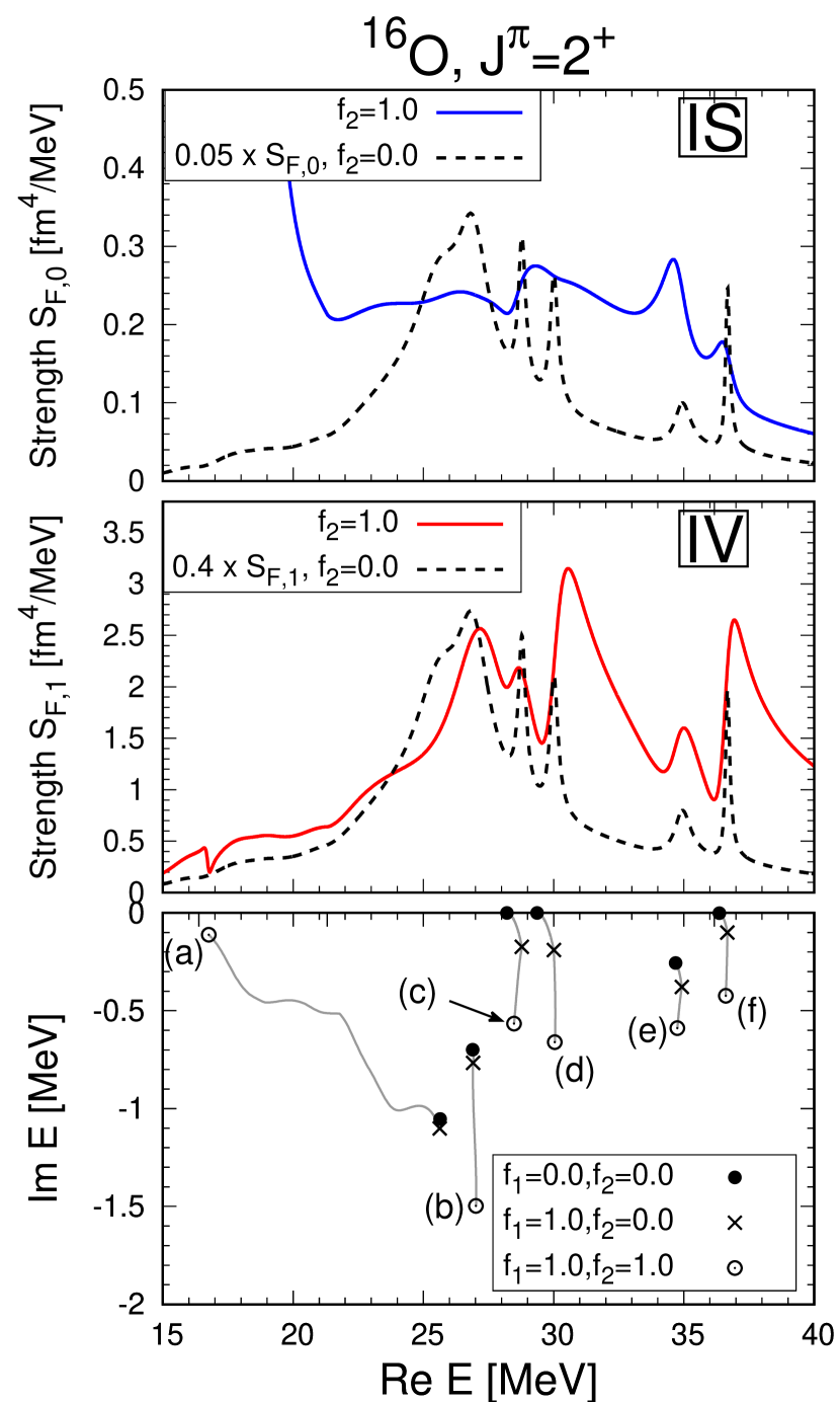
Figure 1: (Color online) The isoscalar and isovector RPA strength functions for the quadrupole excitation of ¹⁶O were shown by the solid blue and red curves in the top and middle panels, respectively. The dashed line shows the RPA strength function calculated with $\kappa_{np}=0$, multiplied by factors $0.05$ and $0.4$ in the top and middle panels, respectively. The trajectories of poles (a)-(f) obtained by solving Eq.(21) varying the constant parameters $f_{1}$ and $f_{2}$ multiplied to the residual interaction are shown in the bottom panel. The open circle ($\circ$), cross ($\times$) and filled circle ($\bullet$) symbols show the position of poles which are calculated by the RPA (i.e., $f_{1}=1$, $f_{2}=1$), RPA with $\kappa_{np}=0$ ($f_{1}=1$, $f_{2}=0$) and unperturbed($f_{1}=0$, $f_{2}=0$) solutions, respectively.(See Table.3.)

III Results and discussions

In the numerical calculations in this paper the same model and parameters as in Ref.JostRPA are used for the Woods-Saxon potential and the residual interaction. The target nucleus was also chosen as a relatively light spherical nucleus, ¹⁶O as before, in order to understand the details of the method and to proceed with the analysis. In this paper, the RPA quadrupole excitation is calculated by adopting $f(r)=r^{2}$ as the external field; the distinction between isoscalar(IS) and isovector(IV) modes is given by the sign of the hole state vector, as given in Eqs. (86) and (87). The ground state properties, the single particle levels and r.m.s radius for neutron and proton of ¹⁶O are shown in Table 1. The configuration of the quadrupole excitations of ¹⁶O and subscription $\alpha$ which is used to describe the matrix elements of the Jost function are shown in Table 2. A minor change regarding the numerical solution method from Ref.JostRPA , but the Newton-Raphson method Rakityansky ; NRM is adopted in this paper to solve Eq.(21) and find the S-matrix poles on the complex energy plane.

Table 3: Values of the S-matrix poles shown in the bottom panel of Fig.1. “Sheet” is the Riemann sheet on which the poles are found. The energy regions given in parentheses are the branch-cut lines of analytical continuation on the real axis with the first Riemann sheet. The “origin” gives the configuration of the single-particle excitation of the poles, calculated with $f_{1}=f_{2}=0.0$.

		S-matrix pole [MeV]
Sheet (branch-cut [MeV])	No.	$f_{1}=f_{2}=1.0$	$f_{1}=1.0,f_{2}=0.0$	$f_{1}=f_{2}=0.0$	origin
		($\circ$ in Fig.1)	($\times$ in Fig.1)	($\bullet$ in Fig.1)
Sheet 1 ($11.95\leq E\leq 16.38$)	–	–	–	–	–
Sheet 2 ($16.38\leq E\leq 16.84$)	(a)	$16.76-i0.11$	$25.62-i1.10$	$25.65-i1.05$	$\pi[f_{7/2}\otimes(p_{3/2})^{-1}]$
Sheet 3 ($16.84\leq E\leq 21.31$)	–	–	–	–	–
Sheet 4 ($21.31\leq E\leq 31.16$)	(b)	$27.02-i1.50$	$26.91-i0.77$	$26.89-i0.70$	$\nu[f_{7/2}\otimes(p_{3/2})^{-1}]$
	(c)	$28.48-i0.57$	$28.78-i0.17$	$28.21$	$\pi[d_{5/2}\otimes(s_{1/2})^{-1}]$
	(d)	$30.47-i0.66$	$30.01-i0.19$	$29.36$	$\nu[d_{5/2}\otimes(s_{1/2})^{-1}]$
Sheet 5 ($31.16\leq E\leq 36.17$)	(e)	$34.75-i0.59$	$34.91-i0.37$	$34.69-i0.26$	$\pi[d_{3/2}\otimes(s_{1/2})^{-1}]$
Sheet 6 ($36.17\leq E$)	(f)	$36.61-i0.42$	$36.67-i0.10$	$36.36-i0.001$	$\nu[d_{3/2}\otimes(s_{1/2})^{-1}]$

In the top and middle panels of Fig.1, the RPA isoscalar and isovector strength functions are shown by the blue and red solid curves, respectively. The dashed curve shows the RPA strength function calculated by ignoring the residual interaction between neutrons and protons. To compare the peak structures of the solid and dashed strength functions in the energy region above 20 MeV, the dashed strength functions were multiplied by 0.05 (top panel) and 0.4 (middle panel). The bottom panel of Fig.1 shows the S-matrix poles and their trajectories obtained by solving Eq.(21). The trajectories were obtained by varying the constants multiplied by the residual interaction in the same way as done in Ref.JostRPA . Depending on the poles, the Riemann sheet to which the poles belong is different; the values of the S-matrix poles and the Riemann sheets to which they belong are shown in Table 3.

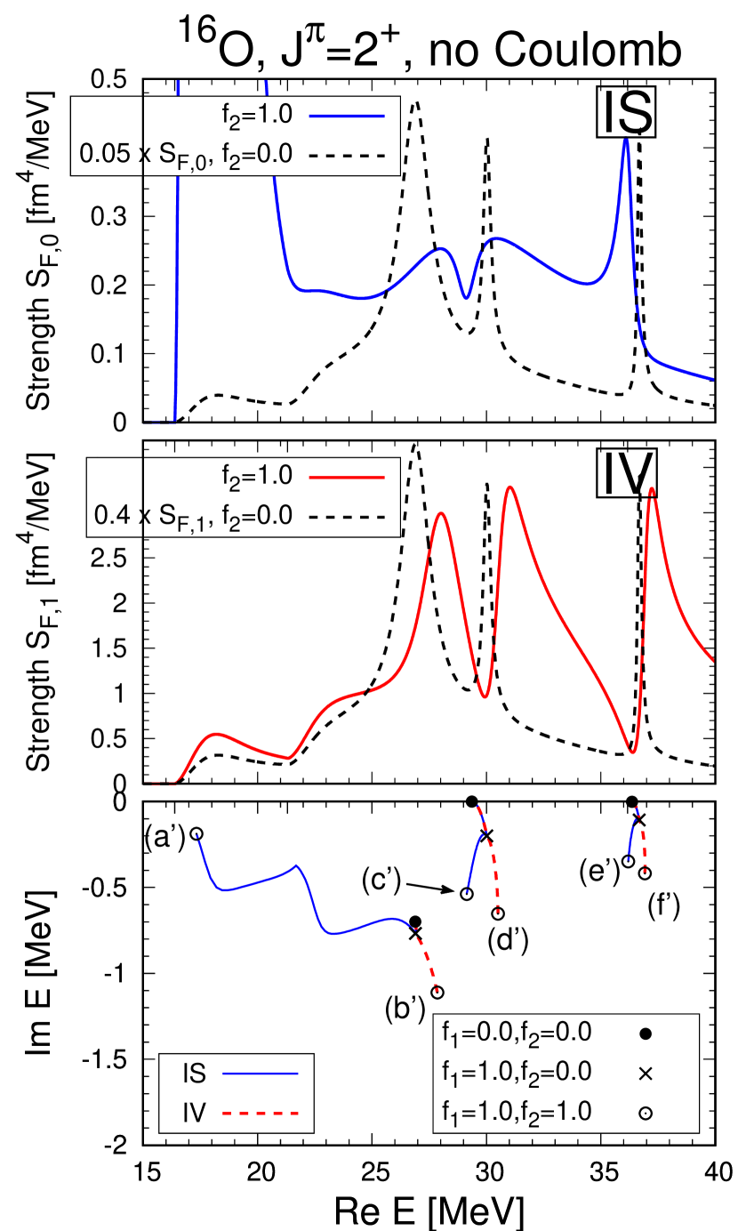
Figure 2: (Color online) The same figure with Fig.1 but calculated without Coulomb interaction. The trajectories of poles are calculated by solving Eq.(107), the positive and negative signs for the isoscalar and isovector modes, respectively. (See. Table.4.)

Basically, isoscalar (IS) and isovector (IV) modes are excitation modes caused by neutron-proton coupling. Therefore, there is no distinction between IS and IV modes in the strength function indicated by the dashed curve in the upper and middle panels, and it can be easily confirmed that the S-matrix poles marked with cross($\times$) symbols in the bottom panel correspond to the peaks of the strength function indicated by the dashed curve.

However, in RPA calculations considering neutron-proton coupling, it is known that IS and IV modes are mixed when the neutron and proton density distributions are different. (Mixing of IS and IV modes occurs even in Z=N nuclei, such as ¹⁶O, due to isospin symmetry breaking by the presence of the Coulomb interaction.)sagawa . It is therefore difficult to find a clear correspondence between the poles and the peaks of the RPA strength function, except for a pole (a), which are clearly isolated from the other poles.

Table 4: Almost the same table as Table 3 for Fig.2. The “mode” shown in the last column indicates the excitation mode (IS: Isoscalar or IV: Isovector) for each pole.

		S-matrix pole [MeV]
Sheet (branch-cut [MeV])	No.	$f_{1}=f_{2}=1.0$	$f_{1}=1.0,f_{2}=0.0$	$f_{1}=f_{2}=0.0$	origin	mode
		($\circ$ in Fig.2)	($\times$ in Fig.2)	($\bullet$ in Fig.2)
Sheet 1 ($16.38\leq E\leq 21.31$)	(a’)	$17.33-i0.19$	$26.90-i0.77$	$26.89-i0.70$	$[f_{7/2}\otimes(p_{3/2})^{-1}]$	IS
Sheet 2 ($21.31\leq E\leq 36.17$)	(b’)	$27.86-i1.11$				IV
	(c’)	$29.14-i0.54$	$30.02-i0.20$	$29.36$	$[d_{5/2}\otimes(s_{1/2})^{-1}]$	IS
	(d’)	$30.50-i0.65$				IV
Sheet 3 ($36.17\leq E$)	(e’)	$36.20-i0.35$	$36.68-i0.11$	$36.36-i0.001$	$[d_{3/2}\otimes(s_{1/2})^{-1}]$	IS
	(f’)	$36.92-i0.42$				IV

For $Z=N$ nuclei, the IS and IV modes can be obtained as independent solutions without mixing if the Coulomb interaction is neglected. Fig.2 is the same as Fig.1 but ignoring the Coulomb interaction. Using Eq.(107), the S-matrix poles can also be obtained independently for the IS and IV modes. The results of Fig.2 and Table 4 show that (a’), (c’) and (e’) are the poles of the IS mode and (b’), (d’) and (f’) are the poles of the IV mode. (a’) and (b’), (c’) and (d’), (e’) and (f’) are IS and IV modes, respectively, originating from the same state due to the effect of residual interaction. In other words, in the case of a pair of poles (a’) of an IS mode and a pole (b’) of an IV mode, for example, the origin of both poles is a pole at $26.89-i0.70$ MeV. Firstly, this becomes a pole existing at $26.90-i0.77$ MeV due to the effect of residual interaction between homologous nucleons. This is then further split into an independent IS-mode pole($17.33-i0.19$ MeV) and an IV-mode pole($27.86-i1.11$ MeV) by the effect of residual interaction between neutrons and protons.

Comparing the positions of the S-matrix poles indicated by open circle symbols($\circ$) in Fig.2 and the peaks of the strength function represented by solid curves, it seems that the real part of the S-matrix poles generally corresponds to the peaks of the strength function, except the IS mode (c’). A comparison of the S-matrix poles in Figs.1 and 2 shows that there is a correspondence. In the presence of the Coulomb interaction, the origin pole separates into two poles due to isospin symmetry breaking, as shown in Fig.1 and Table 3. In the example of the previous pair (a’) and (b’), the origin pole at $26.89-i0.70$ MeV separates into $25.65-i1.05$ MeV and $26.89-i0.70$ MeV poles, which become pole (a) and pole (b) respectively due to residual interaction.

Figure 3: (Color online) Eigenphase shift $\delta^{(1)}_{\alpha}$ obtained by diagonalising the $\mbox{\boldmath$\mathcal{S}$}^{(1)}$ matrix using Eq.(81) (bottom panel) and decomposition of the RPA strength function by the eigenphase shift components (second and third panels). (a)-(f) in the upper figure are the S-matrix poles shown in Fig.1 and Table 3. The imaginary part of the poles is represented by error bars. (i)-(v) show the positions of the K-matrix poles appearing on the real axis of energy. The energy of the K-matrix pole is equivalent to the energy when the eigenphase shift $\delta^{(1)}_{\alpha}$ crosses $\pi/2$. (See Table.5.)

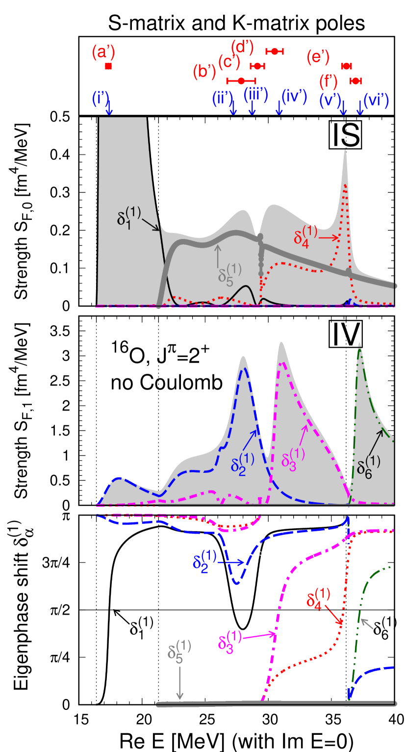
Figure 4: (Color online) The same figure with Fig.3 but calculated without Coulomb interaction.

However, as discussed in Ref.jost-fano ; jost-class , it does not always guarantee that the position of the real part of the S-matrix poles in general reflects or corresponds to the position of the peak of a physical quantity such as the cross section or strength function. This is because the Jost function is essentially a multivalued function of complex energy, so there can be energy shifts caused by the nature of the multivalued function, and if several poles exist in close proximity to each other, there is a superposition of the contributions of the individual poles. There are also background contributions arising from non-resonant continuum state contributions, because interference effects, including Fano effects, also affect the peak structure. Furthermore, there is a mixture of IS and IV modes, so it is not easy to derive conclusions about the correspondence between the peak structure of the strength function and the S-matrix poles and their contributions.

The Gamow shell modelgamow1 ; gamow2 and the complex scaling methodCSM1 ; CSM2 exist as methods which can decompose the contribution of the S-matrix poles in the strength function and cross section. Further extension of the method is underway to apply these methods to our Jost function method. In this paper, we attempt the alternative way for the detailed analysis.

In the previous section of this paper, we derived the S-matrix which satisfies the unitarity associated with the description of the RPA strength function within the framework of RPA theory using the Jost function. The S-matrix which satisfies unitarity can be diagonalised using the unitary matrices as shown in Eq.(81), which provides the eigenphase shifts. Since the unitary transformation is an isometric transformation, the unitary matrix, which diagonalises the S-matrix, can decompose the RPA intensity function into components for each eigenphase shift without changing its magnitude. The poles of the K-matrix, defined using the S-matrix, appear on the real axis of energy and are equal to the energy at which the eigenphase shift crosses $\pi/2$, referred to as the eigenvalue of the Sturm-Liouville problem.

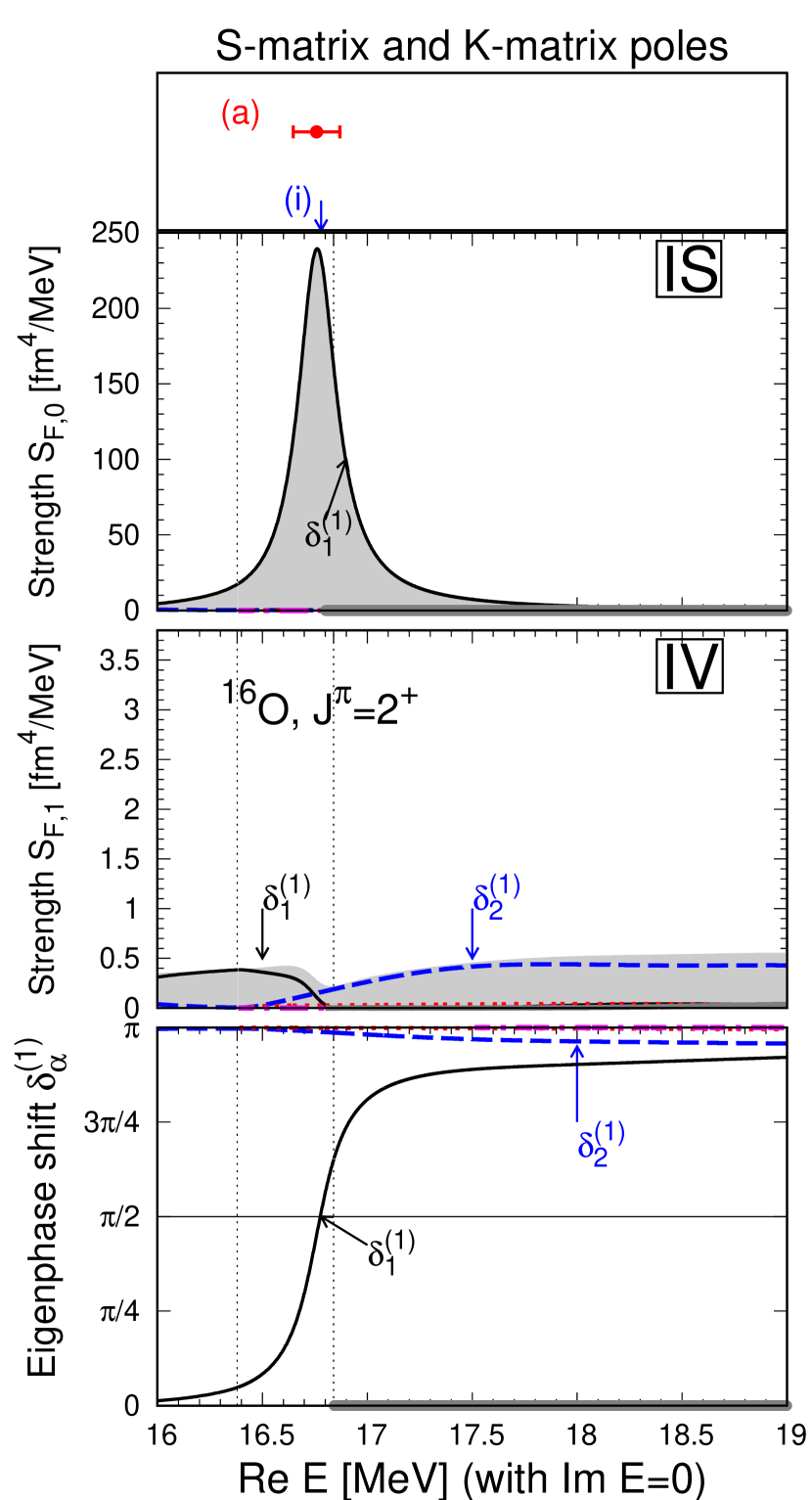
Figure 5: (Color online) Magnified view of the energy region from $16$ MeV to $19$ MeV in Fig.3.

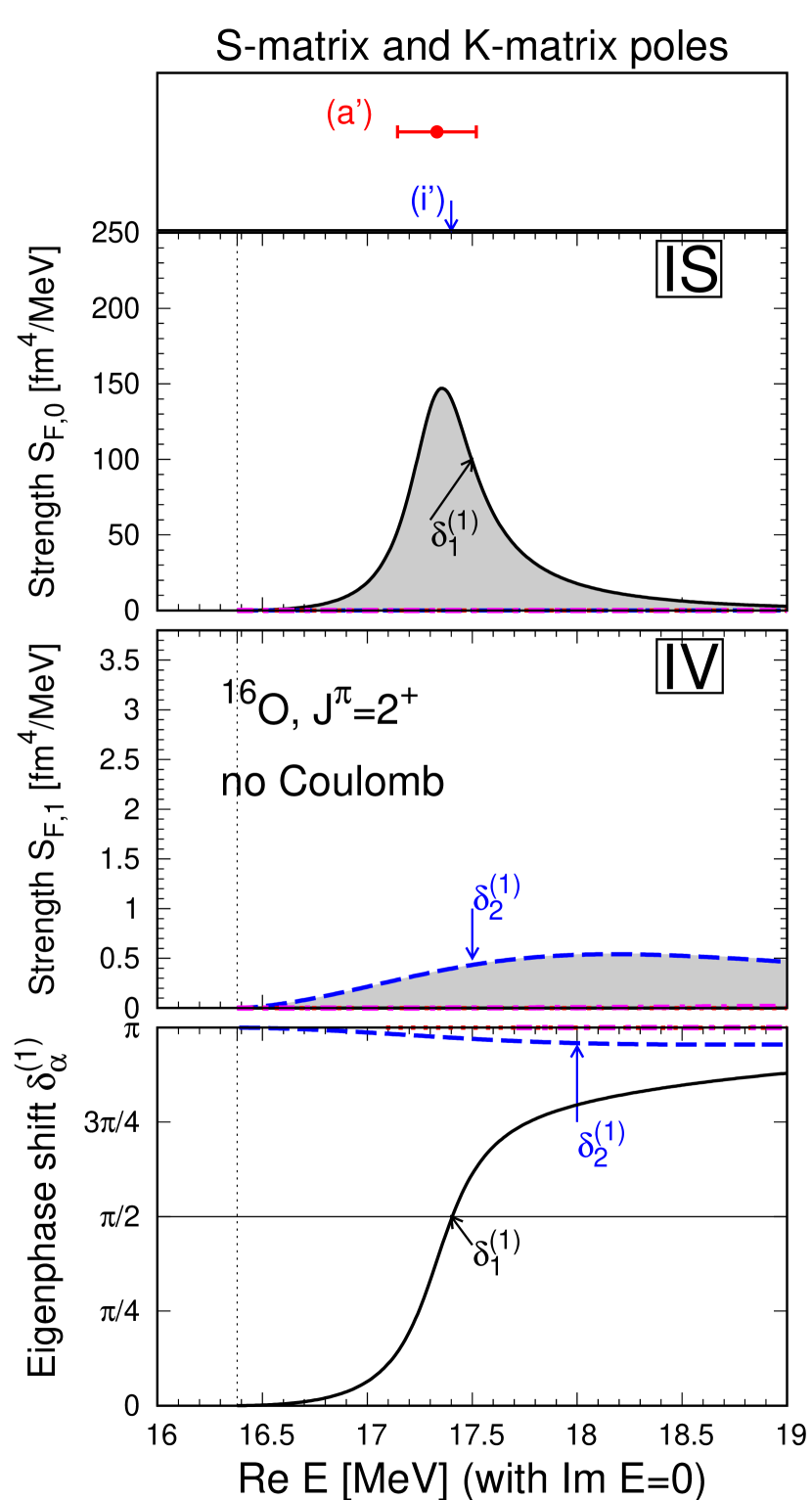
Figure 6: (Color online) Magnified view of the energy region from $16$ MeV to $19$ MeV in Fig.4.

Eigenphase shifts $\delta^{(1)}_{\alpha}$ obtained by diagonalising $\mbox{\boldmath$\mathcal{S}$}^{(1)}$ are shown in the bottom panel of Fig. 3. The first and third rows of the figure show the strength function decomposed into the components giving the eigenphase shifts using Eq.(82). In the top panel of Fig.3, the S-matrix poles (a)-(f) are shown with their imaginary parts represented by error-bars, since it is known that the real part of the S-matrix pole is the resonance energy and the imaginary part is the half-width if it is an isolated pole. (i)-(v) show the location of the K-matrix poles on the real axis of energy. As is clear from the derivation of the S-matrix in the previous section, the size of the S-matrix depends on the energy region of the Riemann sheet shown in Table 3. For example, in the energy region of Sheet 2 ($16.38\leq E\leq 16.84$ MeV), the S-matrix is a $4\times 4$ matrix because $\alpha=1,2,9$ and $10$ are open in the configuration channels given in Table 3. In the case of Sheet 4 ($21.31\leq E\leq 31.16$ MeV), the S-matrix is a $4\times 4$ matrix because $\alpha=1-6,9-14$ channels are open. Energy regions are indicated by dotted vertical lines in Fig. 3. Despite the fact that the eigenphase shift is obtained by diagonalising S-matrices of different sizes in each energy region, the eigenphase shift is obtained as a function of energy, which is continuously connected at the boundaries of the energy region. The components of the strength function per eigenphase shift are also obtained as a function of continuous energy at the boundaries of the energy region, and the sum of all those components reproduces the total strength function (shown as grey-filled area). Note that the “total strength function” is the same as the strength function which can be obtained by using the cRPA method shlomo . The same figure with Fig.3 but calculated without Coulomb interaction is shown in Fig.4. In order to show the first quadrupole exited state clearly, the magnified view of the energy region from $16$ MeV to $19$ MeV of Figs.3 and 4 are shown in Figs.5 and 6, respectively.

If the Coulomb interaction is neglected, the eigenphase shifts shown in Fig.4 can be obtained independently for the IS and IV modes using Eq.(112). As a result, it can be seen that $\delta^{(1)}_{1}$, $\delta^{(1)}_{4}$ and $\delta^{(1)}_{5}$ are the eigenphase shifts of the IS mode, while $\delta^{(1)}_{2}$, $\delta^{(1)}_{3}$ and $\delta^{(1)}_{6}$ are those of the IV mode. These results are also consistent with the results of the component decomposition of the strength function which are shown above the eigenphase shifts. The energy at which the eigenphase shift crosses $\pi/2$ is the K-matrix pole; it is known that if the S-matrix pole is given by a single pole, the energy derivative $\frac{d\delta^{(1)}_{\alpha}}{dE}$ of the phase shift corresponds to the imaginary part of the pole (resonance width) at the energy at which the phase shift crosses $\pi/2$. It is therefore reasonable to consider (ii’) shown in Fig.4 as an independent K-matrix pole which is not associated with the S-matrix pole. For the K-matrix poles, except for (ii’), the correspondence with the S-matrix poles can be found from the difference in energy positions and modes. The results of the correspondence are summarized in the lower half of Table 5.

Table 5: Values of the K-matrix poles and corresponding eigenphase shifts shown in Figs. 3, 5, 4 and 6.

	No.	Eigenphase	K-mat. pole	Corr.	mode
			[MeV]	S-mat.
with Coulomb
	(i)	$\delta_{1}^{(1)}$	$16.78$	(a)	IS
	(ii)	$\delta_{1}^{(1)}$	$27.27$	–	ind.
	(iii)	$\delta_{1}^{(1)}$	$28.05$	(c)
	(iv)	$\delta_{3}^{(1)}$	$30.31$	(d)
	(v)	$\delta_{4}^{(1)}$	$36.80$	(e),(f)
without Coulomb
	(i’)	$\delta_{1}^{(1)}$	$17.40$	(a’)	IS
	(ii’)	$\delta_{1}^{(1)}$	$27.23$	–	ind.
	(iii’)	$\delta_{1}^{(1)}$	$28.72$	(c’)	IS
	(iv’)	$\delta_{3}^{(1)}$	$30.86$	(d’)	IV
	(v’)	$\delta_{4}^{(1)}$	$35.95$	(e’)	IS
	(vi’)	$\delta_{6}^{(1)}$	$37.27$	(f’)	IV

As seen in Fig. 6, the eigenphase shift $\delta^{(1)}_{1}$ gives a very large strength function of the IS first quadrupole excited state around $E=17.40$ MeV of the K-matrix pole (i’); the value of the imaginary part of the S-matrix pole corresponding to $\delta^{(1)}_{1}$ (given in Table 4 shows that the width of this peak is $0.38$ MeV ($=0.19\times 2$). In contrast, despite the presence of the corresponding S-matrix pole (c’) for the K-matrix pole (iii’), $\delta^{(1)}_{5}$ makes only a minor contribution to the strength function of the IS mode around the energy of (iii’) $E=28.72$ MeV. Near this energy, the main contribution is given by the eigenphase shift $\delta^{(1)}_{5}$ (non-resonant continuum state), which has no K-matrix pole and is close to zero. However, the basic shape of the strength function near the K-matrix pole (iii’) is given by the strength function component contributed by $\delta^{(1)}_{1}$. The shape of this strength function $\delta^{(1)}_{1}$ component is asymmetric, which means that quantum interference effects such as the Fano effect may exist. The Fano effect (or Fano resonance) is known as a special quantum interference effect that is universal to quantum many-body systems and is known in atomic physics as the effect that causes autoionisation phenomena fano ; Chu ; moiseyev ; Desrier . As far as the RPA strength function is concerned, its contribution is very small and negligible compared to the first excited state, but as the K-matrix pole (iii’) is a state with a corresponding S-matrix pole (c’), it is expected to give a clear contribution to quantities related to the scattering cross section such as the imaginary part of the T-matrix. However, as our numerical calculations and analysis in this paper focus on the RPA strength function, we can only point out the possible existence of the Fano effect.

The $\delta^{(1)}_{2}$ component in Fig.4 is considered to correspond to the S-matrix pole (b’) because it gives the IV mode contribution from the strength function, but there is no corresponding K-matrix pole. Therefore, the S-matrix pole (d’) is considered to be an independent S-matrix pole which forms the first peak of the IV mode around $E=27$ MeV, but without a corresponding K-matrix pole.

The eigenphase shifts $\delta^{(1)}_{3}$ and $\delta^{(1)}_{6}$ give the K-matrix poles (iv’) and (vi’) with corresponding IV-mode S-matrix poles (d’) and(f’) respectively. These are then the dominant components of the peaks of the IV strength function near the respective K-matrix poles.

The K-matrix pole (v’) given by $\delta^{(1)}_{4}$ has a corresponding S-matrix pole (e’) of the IS mode, forming a sharp IS mode strength function peak which seems to be embedded in the background of the non-resonant continuum state produced by $\delta^{(1)}_{5}$. The $\delta^{(1)}_{4}$ component of the IS strength function also exhibits a very asymmetric shape. It is possible that the Fano effect exists in this case as well, and if it exists, it needs to be clarified in future studies, including what specific phenomena it may be related to.

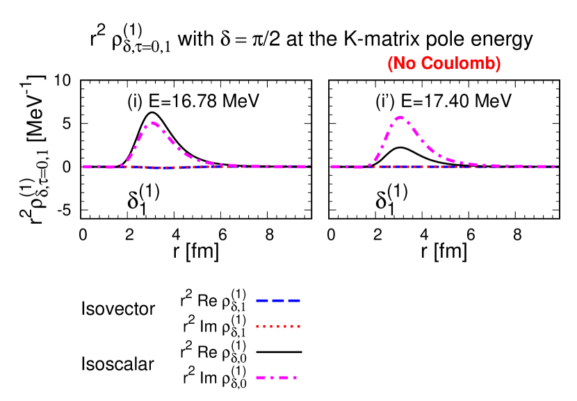
Figure 7: (Color online) The isovector transition density $\rho_{\delta,\tau=1}^{(1)}$ and isoscalar transition density $\rho_{\delta,\tau=0}^{(1)}$ at the first K-matrix pole energy of the eigenphase shift giving the K-matrix poles ((i) and (i’)).

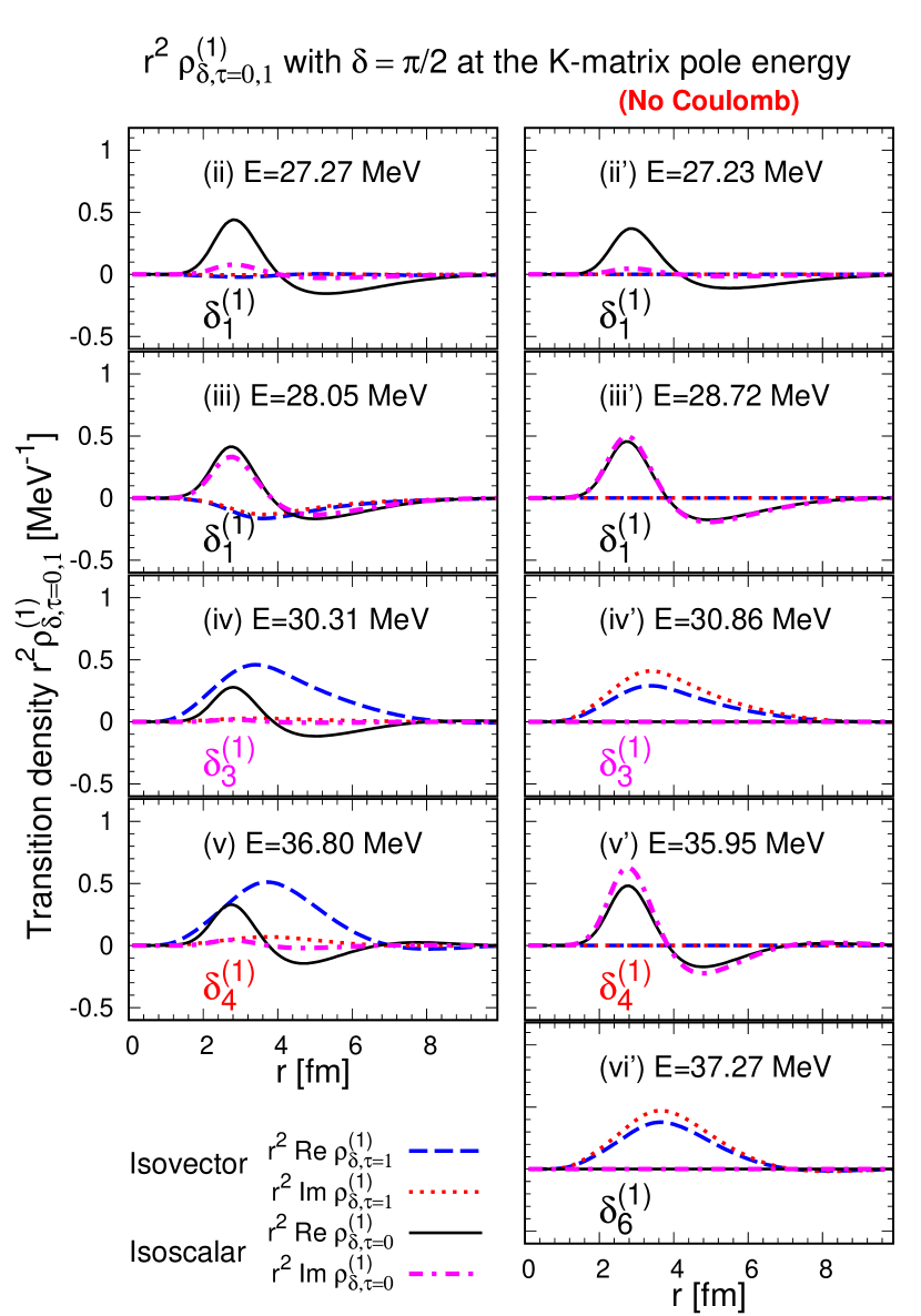
Figure 8: (Color online) The isovector transition density $\rho_{\delta,\tau=1}^{(1)}$ and isoscalar transition density $\rho_{\delta,\tau=0}^{(1)}$ at the K-matrix pole energy of the eigenphase shift giving the K-matrix poles ((ii)-(v) and (ii’)-(vi’)).

The transition density of the eigenphase shift component can be calculated using Eq. (80). Figs.7 and 8 show the transition densities of the eigenphase shift components which give their K-matrix poles at the K-matrix pole energy. The transition densities when neglecting the Coulomb interaction associated with Figs.4 and 6 are shown in the right-hand panels of Figs.7 and 8. Note that the absolute square of the eigenphase shift component of the transition density integrated with respect to $r$ gives the eigenphase shift component of the strength function in Figs.3 and 4, and the sum of all the eigenphase shift components gives the total strength function, by definition (Eq.(82)).

The transition densities of the $\delta^{(1)}_{1}$ component of the K-matrix pole (i’) in Fig. 7, the $\delta^{(1)}_{3}$ component of (iv’) and the $\delta^{(1)}_{6}$ component of (vi’) in Fig. 8 does not have nodes and has a peak near or slightly outside the surface of the nucleus. This shows that the density distribution of neutrons and protons in the nucleus is collectively vibrating, which is one of the typical properties of so-called collective vibration modes.

Since $\delta^{(1)}_{1}$ component of (i’) has only the IS transition density amplitude and $\delta^{(1)}_{3}$ component of (iv’) and $\delta^{(1)}_{6}$ component of (vi’) only the IV transition density amplitude, respectively, this means that (i’) is an IS collective vibration mode and (iv’) and (vi’) are IV collective vibration modes.

The $\delta^{(1)}_{1}$ component of the transition density at the K-matrix pole (ii’) is the transition density with an independent K-matrix pole, the $\delta^{(1)}_{1}$ component of (iii’) and the $\delta^{(1)}_{4}$ component of (v’) with corresponding S-matrix poles (c’) and (e’) respectively. All these transition densities give contributions to the IS mode strength function only. Despite the $\delta^{(1)}_{1}$ component of (iii’) and the $\delta^{(1)}_{4}$ component of (v’) having corresponding S-matrix poles (c’) and (e’) respectively, the transition densities have nodes and do not show clear characteristics of collective vibration modes. In particular, even though the $\delta^{(1)}_{4}$ component of (v’) gives a sharp peak in the shape of the strength function of the IS mode, indicating the possible existence of a clear resonance, the behavior of the transition density does not show any characteristic of collective vibration modes. This could be due to the possibility that resonance and collective mode do not necessarily coincide, or it could be caused by special quantum interference effects such as the Fano effect. This may need to be clarified in future research.

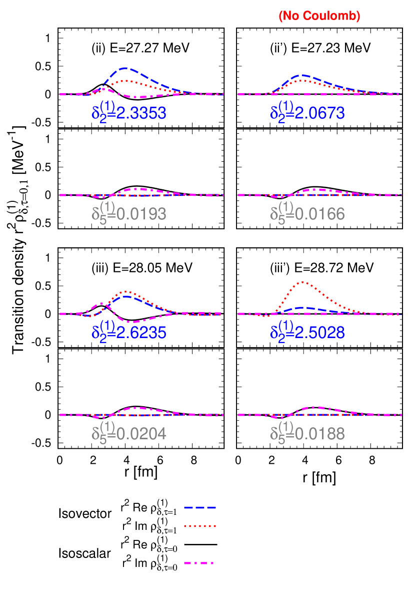
Figure 9: (Color online) The $\delta^{(1)}_{2}$ and $\delta^{(1)}_{5}$ components of the transition densities (IS and IV modes) at K-matrix poles (ii), (iii), (ii’) and (iii’) respectively.

Although $\delta^{(1)}_{2}$ and $\delta^{(1)}_{5}$ are eigenphase shifts which do not give K-matrix poles, they make the main contribution to the IV and IS strength functions near the energies of the K-matrix poles (ii’) and (iii’), respectively. The transition densities of $\delta^{(1)}_{2}$ and $\delta^{(1)}_{5}$ at energies of the K-matrix poles (ii’) and (iii’) are shown in the right-hand panels of Fig. 9. The eigenphase shift $\delta^{(1)}_{2}$ corresponds to the corresponding S-matrix pole (b’), although it does not have a K-matrix pole, and gives the main contribution to the first peak of the IV strength function around 27 MeV, whose transition density exhibits the characteristics of the IV type collective vibration. The eigenphase shift $\delta^{(1)}_{5}$ has neither K-matrix poles nor S-matrix poles but makes the main contribution to the IS strength function above $20$ MeV, and its transition density shows typical non-resonant continuum state properties with nodes and widely spread amplitudes outside the nucleus.

Based on the knowledge gained from the analysis of calculations ignoring the Coulomb interaction that has been carried out so far, the analysis of the RPA strength function including the Coulomb interaction will be carried out from here onwards. The difference caused by the presence or absence of the Coulomb interaction is the change in the single-particle level structure of neutrons and protons due to isospin symmetry breaking and the associated change in density distribution, and the mixing of IS and IV modes caused by it. Comparing the strength functions in Figs.3 and 4, it can be seen that the IS and IV strength functions each contain a mixture of eigenphase shift components which were not present when the Coulomb interaction was ignored. There are also significant changes in the peak structure of the strength function associated with changes in the eigenphase shift.

When the Coulomb interaction is ignored, the sharp peak of the IS strength function, which was formed around $E=36$ MeV with the contribution of the eigenphase shift $\delta^{(1)}_{4}$, is split into two peaks. Focusing on the change in the eigenphase shift $\delta^{(1)}_{4}$ shown in the bottom panels of Figs.3 and 4, $\delta^{(1)}_{4}$ couples with $\delta^{(1)}_{3}$ and $\delta^{(1)}_{6}$ and the K-matrix pole (v’) that existed below the $E=36.17$ MeV threshold disappears. A new K-matrix pole (v) is then formed near the K-matrix pole (vi’) which was formed by $\delta^{(1)}_{6}$ when the Coulomb interaction was ignored. The eigenphase shift $\delta^{(1)}_{4}$ then gives contributions to both IS and IV strength. In fact, the transition density of $\delta^{(1)}_{4}$ at the K-matrix pole (v), shown on the left-hand side of Fig. 8, now has contributions to both IS and IV modes. The peak around $E=35$ MeV of the IS strength function is then formed by the independent S-matrix pole (e), which no longer has a corresponding K-matrix pole. A new peak around $E=35$ MeV also appears in the IV strength function, which is formed by the independent S-matrix pole (e) and is caused by the coupling of the eigenphase shift $\delta^{(1)}_{3}$ with $\delta^{(1)}_{4}$. The fact that the eigenphase shift $\delta^{(1)}_{3}$ is coupled to $\delta^{(1)}_{4}$ can be seen from the transition densities. The transition density of $\delta^{(1)}_{3}$ in the K-matrix pole (iv) shown in the left-hand panel of Fig. 8 now includes characteristics of the transition density of $\delta^{(1)}_{4}$ in (v’) in the right-hand panel, which gives contributions to both IS and IV strength.

The new peak around $E=28$ MeV in the IV strength function is caused by the contribution of the eigenphase shift $\delta^{(1)}_{1}$. This is because $\delta^{(1)}_{1}$ couples with $\delta^{(1)}_{2}$, so that $\delta^{(1)}_{1}$ now gives a contribution to the IV strength. Conversely, by coupling $\delta^{(1)}_{2}$ with $\delta^{(1)}_{1}$, $\delta^{(1)}_{2}$ also makes the contribution to the IS strength when there is the Coulomb interaction, whereas originally it only made the contribution to the IV strength when there was no Coulomb interaction. The same can be seen from the $\delta^{(1)}_{1}$ and $\delta^{(1)}_{2}$ transition densities shown in Figs. 8 and 9. The effect of the Coulomb interaction on the eigenphase shift $\delta^{(1)}_{5}$ component, which is the main component of the IS strength in the energy region above $20$ MeV, is very small. It can be seen from the $\delta^{(1)}_{5}$ transition density shown in Fig. 9 that it hardly changes at all.

The effect of the Coulomb interaction on the IS strength created by the eigenphase shift $\delta^{(1)}_{1}$, which appears as a large and sharp peak at the lowest energy (K-matrix poles (i) and (i’)) shown in Figs.6 and 5, is mainly in peak energy and width. As far as Fig.5 is concerned, there is a slight mixing of the IV mode associated with the coupling with $\delta^{(1)}_{1}$, but the mixing effect with the IV mode is small because it is isolated away from the other poles. The transition density (Fig.7) shows no effect of the mixing of IV modes on this pole, only the characteristics of the IS collective vibration mode.

IV Summary and conclusion

In this paper, we first derived the S-matrix which satisfies the unitarity using the Jost function extended within RPA theory. Considering the properties required to derive the RPA Green’s function in Ref.JostRPA and the symmetric properties of the RPA Green’s function and wave functions in complex energy space in the definition of the RPA strength function, we were able to obtain the “definition of the S-matrix with Jost function” (Eqs. (15) and (44)) which satisfies the unitarity and its associated “scattering wave function” (Eq. (56)). The S-matrix which satisfies the unitarity can be diagonalised by using the unitary matrices, and the diagonal components of the diagonalised S-matrix are expressed in terms of eigenphase shifts. However, the original S-matrix gives a scattering boundary condition where the scattering wavefunction leads through the S-matrix to a free particle state at $r\to\infty$ (the boundary condition imposed to obtain irregular solutions). Since RPA theory describes the excited states of the system in terms of the superposition of particle-hole configurations defined by the mean-field caused by the effects of the residual interaction, Eq.(79) was adopted as the definition of the S-matrix from the idea of the two-potential problem to give the eigenphase shift meaning to describe the RPA excited states.

Applying this method to the quadrupole excitation of the ¹⁶O, the strength function was then decomposed into components for each eigenphase shift, and the correspondence between the eigenphase shift components of the strength function and the S-matrix poles and eigenphase shifts was analyzed. The results show that the components of the RPA strength function corresponding to the eigenphase shift obtained by diagonalising the S-matrix given by Eq.(79) correspond to the S-matrix poles found on the complex energy plane as the zeros of the determinant of the Jost function. Even though the peaks of the strength function correspond to S-matrix poles, there are not necessarily corresponding K-matrix poles, and there are also independent S-matrix poles that do not have K-matrix poles. Also, in the case of poles with simultaneous S- and K-matrix poles, if the eigenphase shift component of the strength function corresponding to the pole exhibits an asymmetric shape, such that the presence of special interference effects such as Fano resonances is suspected, the transition density of that component does not have the characteristics of a collective mode.

The Fano effect is a special quantum interference effect which occurs when a bound or resonant state is coupled to a continuum, and is known in atomic physics as the effect responsible for the phenomenon of autoionisation. In Ref.jost-class , it is shown that in nucleon-nucleus scattering, even in a resonant state where the S- and K-matrix poles exist simultaneously, the scattering wavefunction loses its resonant feature (i.e. the feature that the scattering amplitude is enhanced inside the nucleus) due to the presence of the Fano effect. If a mechanism such as the Fano effect exists in RPA excited states, it is possible that the transition density loses its collective mode character due to this effect. It remains possible, however, that the (resonance) states defined by the S- and K-matrix poles are an independent concept and not directly related to the RPA collective mode. In order to clarify this point, the further study is needed.

It is known that the solutions of the IS and IV modes can be obtained independently in RPA theory for $Z=N$ nuclei such as ¹⁶O if the Coulomb interaction are neglected, and it is confirmed that the Jost function, its determinant and the S-matrix derived in this paper can also be divided into IS and IV modes respectively. Comparing calculations with and without the Coulomb interaction, it can be seen that they cause various effects, such as the coupling of the eigenphase shifts of the IS and IV modes, the disappearance of the K-matrix poles, and the creation of new peaks in the strength function and the splitting of the originally existing peak due to these effects. The eigenphase shift component of the transition density corresponding to a given S-matrix pole is found to give contributions to both IS and IV modes, as the S-matrix pole can no longer be divided into IS and IV modes when the Coulomb interaction is present.

Judging comprehensively from these analyses, the eigenphase shifts obtained by diagonalising the S-matrix derived in this paper can be considered to represent the “RPA excited states” corresponding to the S-matrix poles.

References

- (1) K. Mizuyama, H. Cong Quang, T. Dieu Thuy, and T. V. Nhan Hao, Phys. Rev. C 104, 034606 (2021).
- (2) K. Mizuyama, N. Nhu Le, and T. V. Nhan Hao, Phys. Rev. C 101, 034601 (2020).
- (3) R. Jost and A. Pais, Phys. Rev. 82, 840 (1951).
- (4) Sergai A. Rakityansky, Jost functions in Quantum Mechanics, Springer.
- (5) K. Mizuyama, N. Nhu Le, T. Dieu Thuy, and T. V. Nhan Hao, Phys. Rev. C 99, 054607 (2019).
- (6) K. Mizuyama, N. Nhu Le, T. Dieu Thuy, N. Hoang Tung, D. Quang Tam, and T. V. Nhan Hao, Phys. Rev. C 107, 024303 (2023).
- (7) L. S. Rodberg, R. M. Thaler, Introduction to the Quantum Theory of Scattering, Academic Press (New York and London).
- (8) John Carew and Leonard Rosenberg, Phys. Rev. C 5, 658 (1972).
- (9) Chun-Woo Lee, Phys. Rev. A 58, 4581 (1998).
- (10) W. H. Press, S. A. Teukolsky, W. T. Vetterling, B. P. Flannery, Numerical Receipes in Fortran 77: The Art of Scentific Computing, 2nd edn. (Press Syndicate of the University of Cambridge, New York, 1997).
- (11) H. Sagawa, Prog. Theor. Phys. Suppl. 142, 1 (2001).
- (12) R. Id Betan, R.J. Liotta, N. Sandulescu, T. Vertse Phys. Rev. Lett., 89 (2002), 042501.
- (13) N. Michel, W. Nazarewicz, M. Płoszajczak, K. Bennaceur Phys. Rev. Lett., 89 (2002), 042502.
- (14) Aoyama S., Katō K., and Ikeda K., Prog. Theor. Phys. Suppl. 142, 35 (2001).
- (15) Aoyama S., Myo T., Katō K., and Ikeda K., Prog. Theor. Phys. 116, 1 (2006).
- (16) S. Shlomo and G. Bertsch, Nucl. Phys. A243, 507 (1975).
- (17) U. Fano, Phys. Rev. 124, 1866 (1961).
- (18) Nimrod Moiseyev, Phys. Rep. 302, 211-293 (1998).
- (19) W.-C. Chu and C. D. Lin, Phys. Rev. A 82, 053415 (2010).
- (20) Antoine Desrier, Alfred Maquet, Richard Taïeb, and Jérémie Caillat, Phys. Rev. A 98, 053406 (2018).