1 Introduction

Inflation can solve both the flatness problem and the horizon problem at the same time and also explain temperature fluctuations of the cosmic microwave background (CMB) [1]. It is therefore almost certain that inflation occurred in the early universe. However, a specific mechanism or an origin of a quanta called “inflaton” is still a mystery.

An inflaton is assumed to be a scalar field in typical models, but its potential is, in general, not stable against quantum (gravity) corrections and should be fine-tuned to satisfy constraints of cosmological observations. This problem stems from the fact that radiative corrections on scalar fields cannot be controlled without any assistance of a powerful symmetry.

One way to solve this problem is to consider a higher-dimensional gauge theory, and then a Wilson line phase made of an extra component of a gauge field can become an inflaton whose potential can be determined by the gauge principle. In this scenario, a relevant part of potential is obtained as a function of the Wilson line phase radiatively, taking a finite value [2, 3]. Such an inflaton potential is robust owing to the gauge symmetry and its stability can be guaranteed. A famous five-dimensional (5d) model compactified on a circle $S^{1}$ has been proposed in the name of extranatural inflation [4]. In a similar setup, a model with both a radion and a Wilson line phase has been constructed, and it is shown that the radion is stabilized [5] and the Wilson line phase can be, in most cases, an inflaton [6].

Recently, constraints on cosmological parameters from various observations have become more stringent and inflation models can be selected more rigorously [7]. It is valuable to re-examine whether an extranatural inflation scenario is still valid today or not, in a wide variety of spacetime. It is known that the Randall-Sundrum (RS) warped spacetime can provide rich properties in phenomenological aspects of particle physics. For instance, RS1 model provides a solution of the hierarchy problem of the standard model [8], RS2 model explains the weakness of gravitational force on the TeV brane because the graviton localizes on the Planck brane [9], and gauge-Higgs unification (GHU) models in the warped spacetime can show promise as physics beyond the standard model (BSM) [10, 11, 12, 13]. Hence, it would be favorable if a riddle in cosmology such as inflation could be solved in the same background.

In this paper, we investigate whether inflation in the early universe can be induced by an extra component of a 5d ${\rm U(1)}$ gauge field in the warped background or not. In concrete, we examine whether an effective potential obtained by quantum corrections can act as an inflaton potential by finding parameter regions consistent with Planck 2018 results or not. The RS spacetime contains an orbifold $S^{1}/\mathbb{Z}_{2}$ and a different type of boundary condition called “conjugate boundary condition” can be imposed on fields to survive an extra component of a gauge boson in QED-like models and this enables fields involved in inflation to play a specific role for BSM.

This paper is organized as follows. In the next section, we present a 5d U(1) gauge theory on the warped spacetime. In section 3, we study an extranatural inflation scenario on the warped spacetime based on our model. The last section is devoted to conclusions and discussions.

2 U(1) gauge theory on a warped background

2.1 Randall-Sundrum metric and action integral

The spacetime is assumed to be 5d one with the RS metric given by [8, 9]

$$ds^{2}=g_{MN}dx^{M}dx^{N}=e^{-2\sigma(y)}\eta_{\mu\nu}dx^{\mu}dx^{\nu}+dy^{2},$$ (1)

where $g_{MN}$ ($M,N=0,1,2,3,5$) is the 5d metric, $\eta_{\mu\nu}(=\operatorname{diag}{(-1,1,1,1)})$ ($\mu,\nu=0,1,2,3$) is the four-dimensional (4d) metric, $x^{M}$ and $x^{\mu}$ are 5d and 4d coordinates, respectively, $x^{5}$ is also denoted as $y$, and $\sigma(y)=k|y|$ (for $-\pi R\leq y\leq\pi R$,$\sigma(y+2\pi R)=\sigma(y)$) with a constant $k$ which is related to the cosmological constant $\Lambda_{5}$ in the bulk such as $\Lambda_{5}=-6k^{2}$. The extra space $S^{1}/\mathbb{Z}_{2}$ is expanded in the range of $0\leq y\leq\pi R$, and then $\sigma(y)=ky$ there.

We study a 5d U(1) gauge theory whose action integral is given by

$$S=\int d^{4}x\int_{0}^{\pi R}dy \left\{\sqrt{-g}\left(-\frac{1}{4}g^{MP}g^{NS}C_{MN}C_{PS}+\mathscr{L}_{\rm gf}\right)\right.$$

$$+\det({e^{A}}_{M})\overline{\psi}\left(\varGamma^{A}{e_{A}}^{M}\mathscr{D}_{M}-M_{\psi}-c\sigma^{\prime}(y)\right)\psi\biggl{\}},$$ (2)

where $\sqrt{-g}=\sqrt{-\det{g_{MN}}}$, $g^{MN}$ is the inverse of 5d metric, $C_{MN}=\partial_{M}C_{N}-\partial_{N}C_{M}$ is the field strength made of the 5d U(1) gauge boson $C_{M}$, $\mathscr{L}_{\rm gf}$ is a gauge-fixing term, ${e^{A}}_{M}$ and ${e_{A}}^{M}$ ($A=0,1,2,3,5$) are a fünfbein and its inverse, $A$ is an index of 5d local Lorentz coordinates, $\varGamma^{A}$ are the gamma matrices satisfying the relation $\{\varGamma^{A},\varGamma^{B}\}=2\eta^{AB}(=2\operatorname{diag}{(-1,1,1,1,1)})$, $\psi$ is a 5d fermion with a mass $M_{\psi}+c\sigma^{\prime}(y)$ ($M_{\psi}$ is a $y$-independent bulk mass, $c$ is a $y$-dependent bulk mass coefficient, and $\sigma^{\prime}(y)=d\sigma(y)/dy$), and $\mathscr{D}_{M}$ is a covariant derivative defined by

$$\mathscr{D}_{M}=\partial_{M}+\frac{1}{8}\omega_{AB,M}[\varGamma^{A},\varGamma^{B}]-ig_{5}q_{\psi}C_{M},$$ (3)

using the spin connection $\omega_{AB,M}$ and the gauge boson $C_{M}$. In (3), $g_{5}$ is a 5d gauge coupling, $q_{\psi}$ is a U(1) charge of $\psi$, and each component of $\mathscr{D}_{M}$ is written as

$$\mathscr{D}_{\mu}=\partial_{\mu}-\frac{1}{2}\sigma^{\prime}(y)e_{a\mu}\gamma^{a}\gamma^{5}-ig_{5}q_{\psi}C_{\mu},~{}~{}\mathscr{D}_{y}=\partial_{y}-ig_{5}q_{\psi}C_{y},$$ (4)

where $e_{a\mu}=\eta_{ab}{e^{b}}_{\mu}$ ($\eta_{ab}(=\operatorname{diag}{(-1,1,1,1)})$ and ${e^{b}}_{\mu}$ are the 4d metric and a vierbein in the 4d local Lorentz coordinates, respectively), $\gamma^{a}$ ($a=0,1,2,3$) are the gamma matrices satisfying the relation $\{\gamma^{a},\gamma^{b}\}=2\eta^{ab}(=2\operatorname{diag}{(-1,1,1,1)})$, $a$ and $b$ are indexes of 4d local Lorentz coordinates, $\gamma^{5}(\equiv-i\gamma^{0}\gamma^{1}\gamma^{2}\gamma^{3})$ is 4d chirality operator, and $C_{y}=C_{5}(x,y)$. Here and hereafter $x^{\mu}$ on an argument of fields is denoted as $x$ for short.

2.2 Conjugate boundary conditions

We impose the so-called conjugate boundary conditions (CBCs) on 5d fields, in order to obtain a zero mode of $C_{y}$ after $S^{1}/\mathbb{Z}_{2}$ compactification [14, 15, 16, 17].

The CBCs of $C_{M}(x,y)$ and $\psi(x,y)$ in the Dirac representation are given by

$$C_{M}(x,y+2\pi R)=C_{M}(x,y),\quad C_{\mu}(x,-y)=-C_{\mu}(x,y),\quad C_{y}(x,-y)=C_{y}(x,y),$$ (5)

$$\psi(x,y+2\pi R)=e^{i\beta}\psi(x,y),\quad\psi(x,-y)=\psi^{\rm C}(x,y)\equiv e^{i\theta_{\rm C}}\varGamma^{2}\psi^{*}(x,y),$$ (6)

where $\beta$ is a constant called a twisted phase, the superscript ${\rm C}$ denotes a 4d charge conjugation, $\theta_{\rm C}$ is a real number, and the asterisk means the complex conjugation. Then, the covariant derivatives obey the relations:

$$\left(\partial_{M}+\frac{1}{8}\omega_{AB,M}(x,y+2\pi R)[\varGamma^{A},\varGamma^{B}]-ig_{5}q_{\psi}C_{M}(x,y+2\pi R)\right)\psi(x,y+2\pi R)$$

$$~{}~{}~{}~{}~{}~{}~{}~{}=\left(\partial_{M}+\frac{1}{8}\omega_{AB,M}(x,y)[\varGamma^{A},\varGamma^{B}]-ig_{5}q_{\psi}C_{M}(x,y)\right)\psi(x,y),$$ (7)

$$\left(\partial_{\mu}-\frac{1}{2}\sigma^{\prime}(-y)e_{a\mu}\gamma^{a}\gamma^{5}-ig_{5}q_{\psi}C_{\mu}(x,-y)\right)\psi(x,-y)$$

$$~{}~{}~{}~{}~{}~{}~{}~{}=\left(\partial_{\mu}-\frac{1}{2}\sigma^{\prime}(y)e_{a\mu}\gamma^{a}\gamma^{5}-ig_{5}q_{\psi}C_{\mu}(x,y)\right)^{*}\psi^{\rm C}(x,y),$$ (8)

$$\left(\partial_{-y}-ig_{5}q_{\psi}C_{y}(x,-y)\right)\psi(x,-y)=-\left(\partial_{y}-ig_{5}q_{\psi}C_{y}(x,y)\right)^{*}\psi^{\rm C}(x,y).$$ (9)

Based on the above CBCs and suitable ones for $g_{MN}$ and ${e^{A}}_{M}$, we find that the requirement is fulfilled for $c=0$ that the action integral $S$ should be invariant under the translation $y\to y+2\pi R$ and the $\mathbb{Z}_{2}$ transformation $y\to-y$. U(1) gauge theories with the CBCs own several interesting features. (1) The 4d-components of U(1) gauge boson $C_{\mu}$ have no zero mode, and the U(1) gauge symmetry is explicitly broken by the BCs. (2) The extra component of gauge boson $C_{y}$ can have a zero mode and become a Wilson line phase. (3) 5d fermions can have constant bulk masses. (4) 5d fermions can produce Kaluza-Klein (KK) towers of 4d Majorana fermions.

For later convenience, we change a variable from $y$ to $z=e^{ky}$. Then, the range of $S^{1}/\mathbb{Z}_{2}$ changes from $0\leq y\leq\pi R$ to $1\leq z\leq z_{L}(=e^{k\pi R})$, and (5) and (6) are rewritten by

$$C_{M}(x,z_{L}^{2}z)=C_{M}(x,z),\quad C_{\mu}(x,1/z)=-C_{\mu}(x,z),\quad C_{y}(x,1/z)=C_{y}(x,z),$$ (10)

$$\psi(x,z_{L}^{2}z)=e^{i\beta}\psi(x,z),\quad\psi(x,1/z)=\psi^{\rm C}(x,z)\equiv e^{i\theta_{\rm C}}\varGamma^{2}\psi^{*}(x,z),$$ (11)

respectively.

2.3 Mass spectrum

We examine a zero mode of $C_{y}$ and a mass spectrum of fermion $\psi$. Setting $z=e^{ky}$, the metric (1) is rewritten as

$$ds^{2}=\frac{1}{z^{2}}\left(\eta_{\mu\nu}dx^{\mu}dx^{\nu}+\frac{dz^{2}}{k^{2}}\right).$$ (12)

Then, the action integral is rewritten as

$$S=\int d^{4}x\int_{1}^{z_{L}}dz \left\{\frac{1}{z}\left(-\frac{1}{4k}C_{\mu\nu}C^{\mu\nu}-\frac{k}{2}C_{\mu z}C^{\mu z}+{\check{\mathscr{L}}}_{\rm gf}\right)\right.$$

$$+\left.\frac{1}{k}\,\overline{\check{\psi}}\left(\gamma^{\mu}D_{\mu}+k\gamma^{5}D_{z}-M_{\psi}\right)\check{\psi}\right\},$$ (13)

where ${\check{\mathscr{L}}}_{\rm gf}=\mathscr{L}_{\rm gf}/(kz^{4})$, ${\check{\psi}}=\psi/z^{2}$, $C_{\mu z}=\partial_{\mu}C_{z}-\partial_{z}C_{\mu}$, $C_{z}=C_{y}/(ke^{ky})$, $D_{\mu}=\partial_{\mu}-ig_{5}q_{\psi}C_{\mu}$, $D_{z}=\partial_{z}-ig_{5}q_{\psi}C_{z}$, and $c=0$ is taken by the CBCs.

The Lagrangian density in (13) contains a mixing term of $C_{\mu}$ and $C_{z}$ such as

$$\frac{k}{z}(\partial_{\mu}C_{z})(\partial^{z}C^{\mu})=\left\{\partial_{z}\left(\frac{k}{z}C^{z}\right)\right\}(\partial_{\mu}C^{\mu})+{\rm total~{}derivatives}$$ (14)

and the following gauge-fixing term is introduced, in order to cancel the above mixing term [18],

$$\check{\mathscr{L}}_{\rm gf}=\frac{1}{2\xi k}\left[\partial_{\mu}C^{\mu}-z\xi k\left\{\partial_{z}\left(\frac{k}{z}C^{z}\right)\right\}\right]^{2},$$ (15)

where $\xi$ is a gauge parameter. In this gauge-fixing, the equation of motion of $C_{z}$ is given by

$$\Box_{4}C_{z}-\xi k^{2}\partial_{z}\left\{z\partial_{z}\left(\frac{1}{z}C_{z}\right)\right\}=0,$$ (16)

where $\Box_{4}=\eta^{\mu\nu}\partial_{\mu}\partial_{\nu}$. We now perform the KK mode expansion for $C_{z}$ as

$$C_{z}(x,z)=\frac{1}{\sqrt{k}}\sum_{n=-\infty}^{\infty}h^{(n)}(z)C^{(n)}_{z}(x),$$ (17)

where $h^{(n)}(z)$ are a set of orthogonal functions satisfying $\int_{1}^{z_{L}}\frac{dz}{z}h^{(n)}(z)h^{(m)}(z)=\delta_{nm}$ and $C^{(n)}_{z}(x)$ are 4d fields satisfying the equation $\Box_{4}C^{(n)}_{z}(x)=k^{2}\lambda^{2}_{n}C^{(n)}_{z}(x)$ with constants $\lambda_{n}$. Inserting (17) into eq. (16) with $\xi=-1$, we obtain the eigenvalue equation on $h^{(n)}(z)$:

$$-\frac{d}{dz}\left\{z\frac{d}{dz}\left(\frac{1}{z}h^{(n)}(z)\right)\right\}=\lambda^{2}_{n}h^{(n)}(z).$$ (18)

The function $h^{(0)}(z)$ corresponding to a zero mode obeys eq. (18) with $\lambda_{0}=0$, and it is given by

$$h^{(0)}(z)=az+bz\ln{z},$$ (19)

where $a$ and $b$ are some constants.

To survive $h^{(0)}(z)$, the Neumann boundary condition at both boundaries ($z=1,\,z_{L}$) is imposed, i.e., $\partial(C_{z}/z)/\partial z=0$ or $d(h^{(0)}/z)/dz=0$, which comes from the requirement that surface terms appearing in the derivation of the action should vanish. The condition leads to $b=0$, and the following normalized zero mode is obtained:

$$h^{(0)}(z)=\sqrt{\frac{2}{z^{2}_{L}-1}}~{}\!z\quad\text{for}\ 1\leq z\leq z_{L}.$$ (20)

Next, let us move on to the calculation of KK masses of the fermion $\check{\psi}(x,z)$. In the chiral representation, the equation of motion of $\check{\psi}(x,z)=(\xi_{\rm R}(x,z),\zeta_{\rm L}(x,z))^{\rm T}$ is given by

$$\left(\begin{array}[]{cc}kD_{z}-M_{\psi}&\sigma^{\mu}D_{\mu}\\ \overline{\sigma}^{\mu}D_{\mu}&-kD_{z}-M_{\psi}\end{array}\right)\left(\begin{array}[]{c}\xi_{\rm R}(x,z)\\ \zeta_{\rm L}(x,z)\end{array}\right)=\left(\begin{array}[]{c}0\\ 0\end{array}\right),$$ (27)

where $\sigma^{\mu}=(I,\bm{\sigma})$, $\overline{\sigma}^{\mu}=(-I,\bm{\sigma})$ ($I$ is the $2\times 2$ unit matrix and $\bm{\sigma}(=(\sigma^{1},\sigma^{2},\sigma^{3}))$ are Pauli matrices). We notice that the 4d U(1) gauge boson is absent in $D_{\mu}$, because $C_{\mu}$ have no zero modes due to the CBCs (10). We now perform the KK mode expansion for $\xi_{\rm R}(x,z)$ and $\zeta_{\rm L}(x,z)$ as

$$\xi_{\rm R}(x,z)=\sum_{n=-\infty}^{\infty}f_{\rm R}^{(n)}(z)u_{\rm R}^{(n)}(x),~{}~{}\zeta_{\rm L}(x,z)=\sum_{n=-\infty}^{\infty}f_{\rm L}^{(n)}(z)u_{\rm L}^{(n)}(x),$$ (28)

where $u_{\rm R}^{(n)}(x)$ and $u_{\rm L}^{(n)}(x)$ are 4d spinor fields satisfying the equations $\overline{\sigma}^{\mu}D_{\mu}u_{\rm R}^{(n)}(x)=k\check{\lambda}_{n}u_{\rm L}^{(n)}(x)$ and ${\sigma}^{\mu}D_{\mu}u_{\rm L}^{(n)}(x)=k\check{\lambda}_{n}u_{\rm R}^{(n)}(x)$ with constants $\check{\lambda}_{n}$. Inserting (28) into eq. (27), we obtain a same eigenvalue equation on $f_{\rm R}^{(n)}(z)$ and $f_{\rm L}^{(n)}(z)$:

$$-\left(D_{z}^{2}-\frac{M_{\psi}^{2}}{k^{2}}\right)f^{(n)}(z)=\check{\lambda}_{n}^{2}f^{(n)}(z),$$ (29)

where $f^{(n)}(z)$ represents both $f_{\rm R}^{(n)}(z)$ and $f_{\rm L}^{(n)}(z)$.

Now, we find that $f_{\rm R}^{(n)}(z)$ and $f_{\rm L}^{(n)}(z)$ are expressed by exponent functions, because eq. (29) has a same form as in the case of a flat spacetime. Using (11), $f^{(n)}(z)$ are determined as

$$f^{(n)}(z)=\frac{1}{\sqrt{z_{L}-1}}\exp\left\{i(2\pi n+\beta)\frac{\ln z}{\ln z_{L}^{2}}\right\}$$ (30)

with the relations $f^{(n)}(z_{L}^{2}z)=e^{i\beta}f^{(n)}(z)$ and $f^{(n)}(1/z)={f^{(n)}}^{*}(z)$, and $u_{\rm R}^{(n)}(x)$ and $u_{\rm L}^{(n)}(x)$ turn out to form 4d Majorana spinors. Then, we see that $\psi(x,z)$ obeying CBCs has two degrees of freedom. After integrating over the fifth coordinate in (13), we obtain the KK masses:

$$\left(m^{(\psi)}_{n}(\theta)\right)^{2}=k^{2}\left\{\frac{2\pi n+\beta-q_{\psi}\theta(x)}{2(z_{L}-1)}\right\}^{2}+M_{\psi}^{2},$$ (31)

where the Wilson line phase $\theta(x)$ is defined by

$$\theta(x)\equiv\int_{-\pi R}^{\pi R}dy\,g_{5}C^{(0)}_{y}(x,y)=2\int_{1}^{z_{L}}dz\,g_{5}C^{(0)}_{z}(x,z)=2g_{5}\sqrt{\frac{z^{2}_{L}-1}{2k}}~{}\!\phi(x).$$ (32)

In (32), we use the relation:

$$C^{(0)}_{z}(x,z)=\frac{1}{\sqrt{k}}h^{(0)}(z)C^{(0)}_{z}(x)=\frac{1}{\sqrt{k}}\sqrt{\frac{2}{z^{2}_{L}-1}}~{}\!z\phi(x)$$ (33)

and denote $C^{(0)}_{z}(x)$ as $\phi(x)$ which will be treated as an inflaton later.

2.4 Effective potential

Let us derive the effective potential for the Wilson line phase $\theta(=\theta(x))$. Taking the standard procedure, a $d$-dimensional effective potential involving one degree of freedom at the one-loop level is given by

$$V_{\rm eff}(\theta) =\mp\frac{i}{2}\int\frac{d^{d}p}{(2\pi)^{d}}\ln\left\{p^{2}+m_{n}(\theta)^{2}\right\}$$

$$=\mp\frac{\varGamma(-d/2)}{2(4\pi)^{\frac{d}{2}}}\sum_{n}m_{n}(\theta)^{d}\quad{\rm for}\ \begin{cases}+:\text{boson}\\ -:\text{fermion}\end{cases},$$ (34)

where $m_{n}(\theta)$ are KK masses and $\varGamma(-d/2)$ is the gamma function. Using (31) and the Poisson summation formula, we can get the effective potential involving a fermion $\psi(x,z)$ with two degrees of freedom:

$$\begin{split}V_{\rm eff}(\theta)&=\frac{3k^{4}}{2\{2(z_{L}-1)\}^{4}\pi^{2}}\sum_{n=1}^{\infty}\frac{\cos{\left\{n(\beta-q_{\psi}\theta)\right\}}}{n^{5}}B_{{5}/{2}}(\alpha n)+\cdots,\\ &=\frac{k^{4}}{2\{2(z_{L}-1)\}^{4}\pi^{2}}\sum_{n=1}^{\infty}\frac{\cos{\left\{n(\beta-q_{\psi}\theta)\right\}}}{n^{5}}(\alpha^{2}n^{2}+3\alpha n+3)e^{-\alpha n}+\cdots,\end{split}$$ (35)

where the ellipsis stands for $\theta$-independent terms including infinities, $\alpha={2(z_{L}-1)M_{\psi}}/{k}$ and $B_{{5}/{2}}(\alpha n)$ is a function with $\nu=5/2$ and $z=\alpha n$ defined by

$$B_{\nu}(z)\equiv\frac{2}{\varGamma(\nu)}\left(\frac{z}{2}\right)^{\nu}K_{\nu}(z),\quad B_{\nu}(0)=1.$$ (36)

In (36), $K_{\nu}(z)$ is the modified Bessel function expressed by

$$K_{\nu}(z)=\frac{1}{2}\left(\frac{z}{2}\right)^{-\nu}\int_{0}^{\infty}dt\,t^{\nu-1}\exp{\left(-t-\frac{z^{2}}{4t}\right)}\quad\text{for}\ z\neq 0,\,|\arg{z}|<\frac{\pi}{4}.$$ (37)

We notice that the expression of $V_{\rm eff}(\theta)$ is similar to that of a flat spacetime such as $M^{4}\times S^{1}$.

3 Gauge-Higgs inflation on a warped background

We will now see whether $V_{\rm eff}(\theta)$ given by (35) or its extension including contributions from several fermions can act as an inflaton potential or not.

3.1 Constraints on inflaton potential

The inflaton potential $V(\phi)$ is strictly constrained by cosmological observations. In particular, the allowed region of the tensor-to-scalar ratio $r$ is getting smaller than that in the past. Constraints at the wavenumber $k_{0}=0.002\ {\rm Mpc}^{-1}$ are listed as [7]

$$\text{slow-roll conditions}: \epsilon\equiv\frac{M^{2}_{\rm Pl}}{2}\left(\frac{V^{\prime}(\phi)}{V(\phi)}\right)^{2}\ll 1,\quad|\eta|\equiv M^{2}_{\rm Pl}\left|\frac{V^{\prime\prime}(\phi)}{V(\phi)}\right|\ll 1,$$ (38)

$$\text{e-folding number}: N=\frac{1}{M^{2}_{\rm Pl}}\left|\int_{\phi_{\rm*}}^{\phi_{\rm e}}\frac{V}{V^{\prime}}d\phi\right|>50,$$ (39)

$$\text{scalar power spectrum}: \mathcal{P}_{\mathcal{R}}=\frac{1}{24\pi^{2}M^{4}_{\rm Pl}}\frac{V(\phi_{*})}{\epsilon_{*}}=(2.105\pm 0.030)\times 10^{-9}\quad(68\,\%\,\text{CL}),$$ (40)

$$\text{spectral index}: n_{\rm s}=1-6\epsilon_{*}+2\eta_{*}=0.9661\pm 0.0040\quad(68\,\%\,\text{CL}),$$ (41)

$$\text{tensor-to-scalar ratio}: r=16\epsilon_{*}<0.066\quad(95\,\%\,\text{CL}),$$ (42)

$$\text{vacuum energy}: V(\phi)|_{\text{min.}}=0,$$ (43)

where $M_{\rm Pl}=\sqrt{{\hbar c^{5}}/{8\pi G}}=2.4353\times 10^{18}\ \text{GeV}$, the parameters with $*$ indicate the values at the horizon exit, and $\phi_{\rm e}$ denotes the value of $\phi$ at the end of inflation, which is limited by the conditions $\epsilon_{\rm e}\simeq 1$ and $|\eta_{\rm e}|\simeq 1$. Here, $\epsilon_{\rm e}$ and $\eta_{\rm e}$ are the values of $\epsilon$ and $\eta$ at $\phi_{\rm e}$. The condition (43) corresponds to the fact that the current vacuum energy (dark energy) density is almost zero.

3.2 Model with a single fermion

From (32), let us use $\phi(=f\theta)$ in place of $\theta$, where $f\equiv\sqrt{{2k}/{(z^{2}_{L}-1)}}/(2g_{5})$. Then, the potential is given by

$$V(\phi)=\frac{k^{4}}{2\{2(z_{L}-1)\}^{4}\pi^{2}}\sum_{n=1}^{\infty}\frac{\cos{\left\{n(\beta-q_{\psi}\phi/f)\right\}}}{n^{5}}(\alpha^{2}n^{2}+3\alpha n+3)e^{-\alpha n}+c_{\text{5d}}+\cdots,$$ (44)

where a 5d cosmological constant term $c_{\text{5d}}$ is introduced as a counter term to renormalize the vacuum energy density and to satisfy the condition (43).

A graph of $V(\phi)$ is depicted in Figure 1.

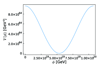
Figure 1: $V(\phi)\ (0<\phi/f<2\pi)$ in the case with $f=7M_{\rm Pl}$, $k=2.465\times 10^{18}\ \text{GeV}$, $\alpha=1$, $\beta=0$, $q_{\psi}=1$ and $2(z_{L}-1)=100$.

Here, it is obtained by summing the function of $n$ in (44) for $n=1$ to 100 numerically, and taking $f=7M_{\rm Pl}$, $k=2.465\times 10^{18}~{}\text{GeV}$, $\alpha=2(z_{L}-1)M_{\psi}/k=1$, $\beta=0$, $q_{\psi}=1$ and $2(z_{L}-1)=100$. In this case, choosing $n_{\rm s}=0.9641$ as an allowed value of $n_{\rm s}$, the values of $\phi_{*}$, $\epsilon_{*}$ and $\eta_{*}$ are determined as $\phi_{*}=1.81\times 10^{19}\ \text{GeV}$, $\epsilon_{*}=0.0040$ and $\eta_{*}=-0.0060$, respectively, from the dependence of $\epsilon,\,\eta$ and $n_{\rm s}$ on $\phi$, and the slow-roll conditions are fulfilled. Then, the tensor-to-scalar ratio becomes $r=0.064$ and a suitable value of the scalar power spectrum is obtained as $\mathcal{P}_{\mathcal{R}}=2.104\times 10^{-9}$ consistent with (40). The $n_{\rm s}$-$r$ contours on the Planck 2018 results and our values are shown in Figure 2. When the inflation ended at $\phi_{\rm e}=5.01\times 10^{19}\ \text{GeV}$ with the e-folding number $N=64$, we find that the conditions $\epsilon_{\rm e}\simeq 1$ and $|\eta_{\rm e}|\simeq 1$ are satisfied with $\epsilon_{\rm e}=1.01$ and $\eta_{\rm e}=1.00$.

Let us change the value of $f$ keeping other parameters unchanged. The tensor-to-scalar ratio $r$ can be reduced when the value of $f$ is smaller. For instance, $f=6M_{\rm Pl}$ with $n_{\rm s}=0.9641$ can produce $r=0.0273$ and this is within the $1\sigma$ region of BICEP2/Keck and BAO constraint, but, in this case, the e-folding number takes a larger value $N=80$. The values of $r$ and $N$ for several values of $f$ are listed in the Table 1. From them, we see that it is difficult to have a plot in the $1\sigma$ region for a model with a single fermion, keeping an appropriate value of $N$. This feature remains almost unchanged even if the values of $\alpha$, $\beta$, $q_{\psi}$ and $n_{\rm s}$ are altered.

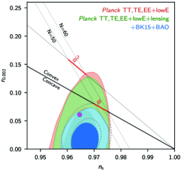
Figure 2: The $n_{\rm s}$-$r$ contours on the Planck 2018 results [7] and the values obtained from our model with a single fermion in the case with $f=7M_{\rm Pl}$. The pink dot represents $(n_{\rm s},r)=(0.9641,0.064)$ with $N=64$. The vertical axis is denoted as $r_{0.002}$ in place of $r$ to represent the observed value of $r$ at the wavenumber $k_{0}=0.002\ {\rm Mpc}^{-1}$.

Table 1: The tensor-to-scalar ratio $r$ and the e-folding number $N$ for several vaules of $f$.

	$f$	$7M_{\rm Pl}$	$6.5M_{\rm Pl}$	$6.3M_{\rm Pl}$	$6M_{\rm Pl}$
$n_{\rm s}=0.9641$	$r$	$0.064$	$0.048$	$0.0041$	$0.0273$
	$N$	$64$	$69$	$72$	$80$
$n_{\rm s}=0.9661$	$r$	$0.055$	$0.039$	$0.031$	$0.017$
	$N$	$69$	$76$	$81$	$94$

3.3 Model with multiple fermions

Next, let us consider a combination of these cos-type potentials. We have now two fermions $\psi_{1}$ and $\psi_{2}$. Each fermion has the values of $\alpha$, $\beta$ and $q_{\psi}$ as shown in Table 2, and then the potential is written as

$$V(\phi)=\frac{3k^{4}}{2\{2(z_{L}-1)\}^{4}\pi^{2}} \left\{\sum_{n=1}^{\infty}\frac{\cos{\{n(-\phi/f)\}}}{n^{5}}B_{{5}/{2}}(\alpha_{1}n)\right.$$

$$\left.+\sum_{n=1}^{\infty}\frac{\cos{\{n({\pi}/{2}-2\phi/f)\}}}{n^{5}}B_{{5}/{2}}(\alpha_{2}n)\right\}+c_{\text{5d}}+\cdots.$$ (45)

Table 2: The values of $\alpha$, $\beta$ and $q_{\psi}$.

	$\alpha$	$\beta$	$q_{\psi}$
$\psi_{1}$	$\alpha_{1}=0.01$	$0$	$1$
$\psi_{2}$	$\alpha_{2}=2.3$	$\frac{\pi}{2}$	$2$

A graph is described in Figure 3.

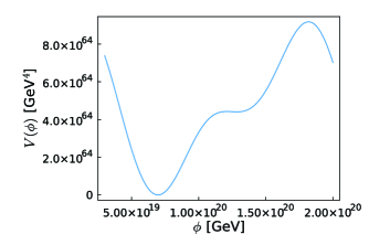
Figure 3: $V(\phi)$ in the case with $f=11M_{\rm Pl}$, $k=2.193\times 10^{18}\ \text{GeV}$ and $2(z_{L}-1)=100$.

Here, it is obtained by summing the function of $n$ in (44) for $n=1$ to 100 numerically, and taking $f=11M_{\rm Pl}$, $k=2.193\times 10^{18}~{}\text{GeV}$ and $2(z_{L}-1)=100$. In this case, choosing $n_{\rm s}=0.9661$ as an allowed value of $n_{\rm s}$, the values of $\phi_{*}$, $\epsilon_{*}$ and $\eta_{*}$ are determined as $\phi_{*}=1.034\times 10^{20}\ \text{GeV}$, $\epsilon_{*}=0.0021$ and $\eta_{*}=-0.011$, respectively, from the dependence of $\epsilon,\,\eta$ and $n_{\rm s}$ on $\phi$, and the slow-roll conditions are fulfilled. Then, the tensor-to-scalar ratio becomes $r=0.034$ and a suitable value of the scalar power spectrum is obtained as $\mathcal{P}_{\mathcal{R}}=2.106\times 10^{-9}$ consistent with (40). When the inflation ended at $\phi_{\rm e}=6.63\times 10^{19}\ \text{GeV}$ with the e-folding number $N=70$, we find that the conditions $\epsilon_{\rm e}\simeq 1$ and $|\eta_{\rm e}|\simeq 1$ are satisfied with $\epsilon_{\rm e}=1.00$ and $\eta_{\rm e}=1.01$. In this way, this type of potential can give a smaller value of $r$.

Let us change the value of $n_{\rm s}$ keeping $f$ unchanged. Taking $n_{\rm s}=0.9641$ as an allowed value of $n_{\rm s}$, the values of $\phi_{*}$, $\epsilon_{*}$ and $\eta_{*}$ are determined as $\phi_{*}=1.025\times 10^{20}\ \text{GeV}$, $\epsilon_{*}=0.00245$ and $\eta_{*}=-0.0106$, respectively. Then, we have $r=0.039$ with $N=65$ and hence even smaller $N$ can be achieved. The $n_{\rm s}$-$r$ contours on the Planck 2018 results and our values are shown in Figure 4.

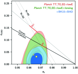
Figure 4: The $n_{\rm s}$-$r$ contours on the Planck 2018 results [7] and the values obtained from our model with two fermions in the case with $f=11M_{\rm Pl}$. The bigger and smaller dots represent $(n_{\rm s},r)=(0.9661,0.034)$ with $N=70$ and $(0.9641,0.039)$ with $N=65$, respectively. The vertical axis is denoted as $r_{0.002}$ in place of $r$, as is the case with Figure 2.

In the same way, we can find a model with more fermions which can give an $n_{s}$-$r$ plot inside the $1\sigma$ region. For instance, using three fermions $\psi_{1}$, $\psi_{2}$ and $\psi_{3}$ with $\alpha$, $\beta$ and $q_{\psi}$ listed in Table 3, we can describe a graph of the potential $V(\phi)$ in Figure 5 and obtain $\phi_{*}=9.30\times 10^{19}\ \text{GeV}$, $\epsilon_{*}=0.0025$, $\eta_{*}=-0.010$, $\mathcal{P}_{\mathcal{R}}=2.103\times 10^{-9}$ and $r=0.040$ for $f=10M_{\rm Pl}$, $k=2.006\times 10^{18}~{}\text{GeV}$, $2(z_{L}-1)=100$ and $n_{\rm s}=0.9641$. In this case, the inflation ended at $\phi_{\rm e}=6.28\times 10^{19}\ \text{GeV}$, $\epsilon_{\rm e}=1.00$ and $\eta_{\rm e}=0.98$ with the e-folding number $N=66$.

Table 3: The values of $\alpha$, $\beta$ and $q_{\psi}$.

	$\alpha$	$\beta$	$q_{\psi}$
$\psi_{1}$	$0.01$	$0$	$1$
$\psi_{2}$	$2.1$	$\frac{\pi}{2}$	$2$
$\psi_{3}$	$2.1$	$\frac{3\pi}{2}$	$1$

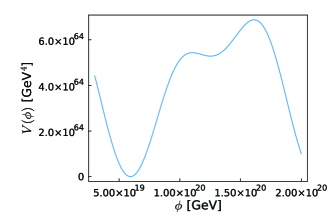
Figure 5: $V(\phi)$ in the case with $f=10M_{\rm Pl}$, $k=2.006\times 10^{18}\ \text{GeV}$ and $2(z_{L}-1)=100$.

4 Conclusions and discussions

We have investigated whether inflation in the early universe can be induced by an extra component of a 5d ${\rm U(1)}$ gauge field coupled to fermions in the RS warped spacetime or not. Imposing CBCs on fields involved in inflation, we have shown that the one-loop effective potential for a Wilson line phase obtained by quantum corrections can behave as an inflaton potential by finding parameter regions consistent with Planck 2018 results. Our model shares basic properties with higher-dimensional models on a flat spacetime, e.g., a potential is generated radiatively, and is robust owing to the gauge symmetry, and then a model has a predictability for physics on inflation.

Both models with a single fermion and multiple fermions have allowed regions of parameters consistent with Planck 2018 results. The former model can give an $n_{\rm s}$-$r$ plot inside the $2\sigma$ region of BICEP2/Keck and BAO constraint, but it is difficult to get them into the $1\sigma$ region while keeping an appropriate value of e-folding number. The latter cos-combined models can reduce the value of the tensor-to-scalar ratio $r$ within the 1$\sigma$ region with a suitable e-folding number.

The remaining issues and future prospects are as follows.

There is a fine-tuning problem that the (initial) vaules of $\phi$ and other parameters should be chosen in order to make $\phi$ as an inflaton work well. It would be better if they are determined from a fundamental theory. Or we would have to rely on the anthropic principle in the framework of multiverse.

While an inflaton can be treated independently of visible particles in our model, this feature can induce a problem how a reheating at the end of inflation occurs in the absence of couplings between the inflaton and the standard model particles at the tree level due to a mismatch of boundary conditions on $S^{1}/\mathbb{Z}_{2}$ [16].

It is necessary to consider contributions of a radion and/or modulus in order to identify an inflaton. In concrete, it is essential to study their stabilization and how inflation can be realized in a system with such several scalar fields including a Wilson line phase on the RS warped background.

It would be wonderful to construct a more realistic higher-dimensional gauge theory which solves riddles of particle physics and cosmology on a similar footing. More specifically, it would be fantastic that, in a system governed by the gauge principle, there are several Wilson line phases originated from extra components of gauge bosons, which behave as Higgs boson, an inflaton, a dark matter and so forth. A top-down approach would be useful to construct such a model in a more unified form. Superstring theory, for instance, provides many scalar and vector fields, and possesses many candidates of Higgs boson, an inflaton, a dark matter and so on. Hence, it is intriguing to investigate how a 5d effective theory on the warped geometry can be realized in such a top-down framework.

References

- [1] D. H. Lyth and A. Riotto, “Particle physics models of inflation and the cosmological density perturbation”, Phys. Rept. 314 , 1 (1999), arXiv:hep-ph/9807278, and references therein.
- [2] Y. Hosotani, “Dynamical Mass Generation by Compact Extra Dimensions”, Phys. Lett. B126, 309 (1983).
- [3] Y. Hosotani, “Dynamics of Nonintegrable Phases and Gauge Symmetry Breaking”, Annals. Phys. 190, 233 (1989).
- [4] N. Arkani-Hamed, H.-C. Cheng, P. Creminelli, and L. Randall, “Extranatural Inflation”, Phys. Rev. Lett. 90, 221302 (2003), arXiv:hep-th/0301218.
- [5] Y. Abe, T. Inami, Y. Kawamura, and Y. Koyama, “Radion stabilization in the presence of a Wilson line phase”, Prog. Theor. Exp. Phys. 2014, 073B04 (2014), arXiv:1404.5125 [hep-th].
- [6] Y. Abe, T. Inami, Y. Kawamura, and Y. Koyama, “Inflation from radion gauge-Higgs potential at Planck scale”, Prog. Theor. Exp. Phys. 2015, 093B03 (2015), arXiv:1504.06905 [hep-th].
- [7] N. Aghanim et al. (Planck), “Planck 2018 results. VI. Cosmological parameters”, Astron. Astrophys. 641, [Erratum: Astron.Astrophys. 652, C4 (2021)], A6 (2020), arXiv:1807.06209 [astro-ph.CO].
- [8] L. Randall and R. Sundrum, “A Large mass hierarchy from a small extra dimension”, Phys. Rev. Lett. 83, 3370-3373 (1999), arXiv:hep-ph/9905221.
- [9] L. Randall and R. Sundrum, “An Alternative to compactification”, Phys. Rev. Lett. 83, 4690-4693 (1999), arXiv:hep-ph/9906064.
- [10] A. D. Medina, N. R. Shah, and C. E. M. Wagner, “Gauge-Higgs Unification and Radiative Electroweak Symmetry Breaking in Warped Extra Dimensions”, Phys. Rev. D 76, 095010 (2007), arXiv:0706.1281 [hep-ph].
- [11] Y. Hosotani, K. Oda, T. Ohnuma, and Y. Sakamura, “Dynamical Electroweak Symmetry Breaking in SO(5) U(1) Gauge-Higgs Unification with Top and Bottom Quarks”, Phys. Rev. D 78, [Erratum: Phys. Rev.D 79, 079902 (2009)], 096002 (2008), arXiv:0806.0480[hep-ph].
- [12] Y. Hosotani, “New dimensions from gauge-Higgs unification”, PoS CORFU2016, 026 (2017), arXiv:1702.08161 [hep-ph].
- [13] S. Funatsu, H. Hatanaka, Y. Hosotani, Y. Orikasa, and N. Yamatsu, “CKM matrix and FCNC suppression in SO(5)U(1)SU(3) gauge-Higgs unification”, Phys. Rev. D 101, 055016 (2020), arXiv:1909.00190 [hep-ph].
- [14] A. Hebecker and J. March-Russell, “The structure of GUT breaking by orbifolding”, Nucl. Phys. B 625, 128-150 (2002), arXiv:hep-ph/0107039.
- [15] N. Haba, Y. Kawamura, and K.-y. Oda, “Dynamical Rearrangement of Theta Parameter in Presence of Mixed Chern-Simons Term”, Phys. Rev. D 78, 085021 (2008), arXiv:0803.4380 [hep-ph].
- [16] Y. Abe, Y. Goto, Y. Kawamura, and Y. Nishikawa, “Conjugate boundary condition, hidden particles, and gauge-Higgs inflation”, Mod. Phys. Lett. A 31, 1650208 (2016), arXiv:1608.06393 [hep-ph].
- [17] K. Kojima and Y. Okubo, “Early dark energy from a higher-dimensional gauge theory”, Phys. Rev. D 106, 063540 (2022), arXiv:2205.13777 [astro-ph.CO].
- [18] C. Caki, S. Lombardo, and O. Telem, “TASI Lectures on Non-supersymmetric BSM Models”, Proceedings, Theoretical Advanced Study Institute in Elementary Particle Physics : Anticipating the Next Discoveries in Particle Physics (TASI 2016): Boulder, CO, USA, June 6-July 1, 2016 , edited by R. Essig and I. Low (WSP, 2018), 501-570, arXiv:1811.04279 [hep-ph].