DyCE: Dynamic Configurable Exiting
for Deep Learning Compression and Scaling

Abstract

Modern deep learning (DL) models necessitate the employment of scaling and compression techniques for effective deployment in resource-constrained environments. Most existing techniques, such as pruning and quantization which primarily aim to generate reduced complexity versions of models through either lowering computational precision or eliminating insignificant elements, are generally static. On the other hand, dynamic compression methods, such as early exits, reduce complexity by recognizing the difficulty of input samples and allocating computation as needed. Dynamic methods, despite their superior flexibility and potential for co-existing with static methods, pose significant challenges in terms of implementation due to any changes in dynamic parts will influence subsequent processes. Moreover, most current dynamic compression designs are monolithic and tightly integrated with base models, thereby complicating the adaptation to novel base models. This paper introduces DyCE, an dynamic configurable early-exit framework that decouples design considerations from each other and from the base model. Utilizing this framework, various types and positions of exits can be organized according to predefined configurations, which can be dynamically switched in real-time to accommodate evolving performance-complexity requirements. We also propose techniques for generating optimized configurations based on any desired trade-off between performance and computational complexity. This empowers future researchers to focus on the improvement of individual exits without latent compromise of overall system performance. The efficacy of this approach is demonstrated through image classification tasks with deep CNNs. DyCE significantly reduces the computational complexity by 23.5% of ResNet152 and 25.9% of ConvNextv2-tiny on ImageNet, with accuracy reductions of less than 0.5%. Furthermore, DyCE offers advantages over existing dynamic methods in terms of real-time configuration and fine-grained performance tuning.

I Introduction

Deep learning (DL) models have exhibited success across a multitude of applications. Nonetheless, they require substantial computations within a short timeframe, which presents significant challenges for deployment on resource-constrained devices, such as Internet of Things (IoT) devices and smartphones. These devices, with their limited computing and memory resources, struggle to accommodate the deployment of large DL models. In addition, the run-time latencies and power consumption would be unacceptable when large DL models are deployed in such environments. Even resource-rich systems, such as data centers, contend with issues regarding energy consumption[1]. Therefore, optimizing model complexity is a critical prerequisite for implementing DL techniques on practical systems.

Various model compression and optimization strategies, like quantization [2] and pruning [3][4], have been introduced to address this complexity concern. Despite their success to varying degrees, they frequently overlook the impact of the difficulty of input data while optimizing model complexity. In practice, input data can range in difficulty levels, some instances being more challenging than others. Difficult input samples might necessitate deep models for acceptable outcomes, while easier inputs might suffice with smaller (shallower) DL models. However, most existing applications use a static data path for all inputs, thereby wasting computational resources on simpler inputs. As a result, dynamic compression techniques are more suitable for assigning computational resources according to the difficulty of each input sample. Early exit [5, 6] is one of the most promising dynamic techniques due to its straightforward logic and broad flexibility. Typically, several auxiliary exiting networks are connected to the models, aiming to output from intermediate points. The computation ceases at the first exit, where the output satisfies an acceptability criteria.

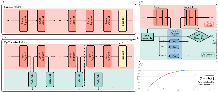
Figure 1: An overview of DyCE system. (a) is the original deep learning model. (b) is the model when DyCE is applied. The backbone of the original model (shown in red) is divided into segments, and multiple early exits (shown in blue) are attached to the end of each segment. The logic of exiting controllers is illustrated in (c). If the confidence level of an output from the exit point is greater than its associated threshold, the inference will complete immediately. Otherwise, the output of the previous backbone segment will be passed to the next segment. The exit select ($k_{n}$) and corresponding thresholds ($t_{n}$) are from the selected configuration. These configurations are pre-defined to adapt varying performance-complexity targets. Red dots in (d) denote configurations that are available in real-time.

Designing an early exit system necessitates answering three critical questions: (1) How to construct efficient exit networks? (2) Where should the exits be positioned? and (3) When should the system exit? However, solutions to any one of these questions could affect the others, thereby making the design process complex. Furthermore, most existing designs are dedicated to specific base models, often requiring a complete system redesign for the adaptation to any new base models.

In response to these challenges, we introduce DyCE, a Dynamic Configurable Exiting framework. It supports scaling the model in real-time to adapt varying demands. DyCE only requires designers to attach arbitrary exits to an existing base model at arbitrary positions. The search algorithms in the proposed framework will identify the optimal combination of exits and exit conditions for a given performance-complexity target. Thus, questions (2) and (3) are disassociated from question (1), enabling designers to focus on single exit performance without any potential adverse effects on the overall system. Figure 1 provides an overview of the proposed system. The DyCE system can be outlined in three components.

1. Early exits (labelled in blue): These are represented by various exit functions attached to the hidden layers of the original model, facilitating an early estimate of the final result. If the output produced at an exit is deemed satisfactory, the inference process concludes at that early layer.

2. A base DL model (labelled in red): DyCE does not necessitate re-training or fine-tuning of the base model but only requires the base model to be divisible along its depth, which is the case commonly found in most DL models. Thus, the proposed compression system has the significant advantage of being independent of the original model in practical implementations.

3. The exit controller (labelled in green): This is a major difference between DyCE and other early exit systems. It features a configurable exit controller wherein the exit selection and acceptance criteria are controlled by pre-configured configurations generated via search algorithms to meet any performance-complexity targets.

In real-world scenarios, performance requirements can vary over time. Using static compression methods that generate fixed model variants necessitates the replacement of entire models when performance targets shift. This requires hardware devices to store multiple compressed variants of the same model and spend significant resources to re-load different models with varying compression rates into memory. In contrast, the DyCE system can be effortlessly reconfigured on-the-fly by simply switching configurations, allowing for real-time adaptation of model compression rate. This enables the dynamic selection of model performance and complexity trade-off points, gives broad flexibility to the DL model, and ensures the full restoration of the original performance when necessary.

The main contributions of this paper are summarized as follows:

1. DyCE Framework: We introduce DyCE, a configurable early-exit-based framework, which can be applied and retrofitted to any existing DL models so as to scale and compress the model dynamically.

2. Real-time Adaptability: The proposed approach enables run-time selection of complexity-accuracy tradeoff points to adapt to varying practical demands. Furthermore, it is compatible with a wide range of deep learning models and other compression methods.

3. Decoupled Design: DyCE decouples the design considerations for creating an early-exit system, simplifying the design process. This design separation allows for focused improvements on individual exits while ensuring systematic performance by DyCE.

4. Search Algorithms: The proposal of two search algorithms for generating configurations suitable for DyCE. These configurations encompass optimized plans detailing which exiting functions to employ and their associated thresholds, catering to different trade-off targets.

For evaluating compression performance, we present the results from an image classification task using ImageNet[7]. The results indicate that DyCE, even without a customised exit network design, can adequately harness the potential of attached exits to achieve competitive performance.

The rest of this paper is structured as follows: Section II reviews the related compression and scaling methods. Section III discusses the inference process proposed in DyCE. Section IV explores considerations in the design of exit networks. Section V introduces the search algorithm proposed for generating configurations. Finally, the experimental results are discussed in Section VI.

II Related Work

TABLE I: Feature comparison between the proposed method and related work

[b] Category Method Work No Extra Network Loosely Coupled¹ No Backbone Training Required Post-training Configurable Real-time Configurable Fine-grained Tuning Dynamic Early Exit DyCE × ✓ ✓ ✓ ✓ ✓ BranchyNet[5] × × × ×² ײ ײ MSDNet[8] MSNet[9] × × × ×² ײ ײ Chen et al.[10] EPNet[11] × × × × × × Layer Skipping SkipNet[12] × × × × × × Channel Skipping RNP[13] × × × × × × Static Architecture Scaling[14][15] ✓ × × × × × Quantization[16] ✓ ✓ ✓ ✓ × × Pruning[3] ✓ ✓ ✓ ✓ × ×

• The method is not majorly relying on specific model architecture or task.

• Support is possible if our proposed method is applied.

Model compression and scaling can be achieved using static or dynamic methods. Static methods typically apply reductions to model structure and weights, while dynamic methods adapt to each individual input sample [17]. We have reviewed and categorized mainstream model compression and scaling techniques, summarizing the primary distinctions in Table I.

II-A Static Methods

Architecture Scaling, an integral part of modern model architectures, allows for the scaling of architectures into different versions [14][15] by modifying the number of repeating components. However, this scaling is coarse-grained, and each version of the model must be trained from scratch.

Quantization [16] is a prevalent compression technique that uses fewer bits to represent network weights or activations. Pruning [3][4] is another common approach that removes redundant weights from a trained neural network. Both these methods can be applied during pre-training or post-training phases, thereby allowing for compressing models to different scales without the need for retraining.

II-B Dynamic Methods

Dynamic compression methods allocate computational resources based on the complexity of each input sample. The Early Exit strategy is a dynamic compression technique that enables “easy” samples to exit at shallow layers, avoiding the execution of deeper network segments. This concept was initially introduced by BranchyNet [5] with confidence-based exits, where computation terminates if the confidence of a classifier exceeds a threshold. Subsequent studies such as FastBERT [18] and PersEPhonEE [19] have extended this confidence-based method across various applications. In these methods, the exit propensity is controlled by external thresholds, thereby enabling post-training or real-time configuration. Alternatively, some research uses policy networks rather than thresholds to control exits [10][11]. These policy networks are trained for specific compression targets, offering improved performance, albeit with less flexibility after training completion.

Other work, such as MSDNet [8] and MSNet [9], achieves high performance by enabling communication among exits at different resolutions. Compared to standard fixed network models, these approaches offer dynamic compression but necessitate task-specific designs. i.e. these approaches cannot be used to retrofit scalability into an existing base model network.

Apart from early exits, which skip all subsequent layers, Layer Skipping [12] is a method that skips some intermediate layers while retaining the remaining model segments. There are also strategies involving Channel Skipping [13], which omits only certain parts of a layer during runtime. Designing and training models that can adapt to skipped intermediate parts present significant challenges, making these methods less prevalent than the early exit approach.

III Inference with Early Exits

An early-exit system can be implemented in various ways. In this section, we outline the inference process employed by DyCE. The runtime component of DyCE is a rapid inference system based on early exits, which dynamically reduces overall computation during model inference. This system facilitates exits at multiple layers on the base model in accordance with a pre-defined configuration. When inference computation reaches at an exit point, the process will terminate if the model exhibits confidence in the preliminary prediction. Hence, more computations are allocated to inputs that cause the exits to have less confidence regarding early-exit decisions, i.e. difficult inputs, while easy inputs are mostly exited at early stages. Additionally, this system can switch configurations at runtime to achieve dynamic scaling.

III-A Runtime Architecture

To illustrate the run-time architecture of DyCE, we start with a pre-trained network (i.e. the base model), e.g., ResNet. Further, the model is divided into different segments, and exit networks are attached to each of them. These exits are trained and grouped into various configurations to obtain the required trade-off. These ideas are now formally defined in the following sub-sections.

Figure 2: Backbone segments and attached exits. At run-time one of $K_{n}$ possible exits will be applied to the output of the $n^{\text{th}}$ segment.

III-A1 Backbone Segments

A deep neural network can usually be considered as two parts: a backbone for feature extraction and a small network at the end for computing the final output. The backbone part is typically stacked as multiple dividable layers. Hence, we consider that the backbone of a pre-trained network is divided into $N$ segments. The nature of this segmentation could be fine or granular, and we denote the output of the $n^{\text{th}}$ segment (and the input to $(n+1)^{\text{th}}$) as $\boldsymbol{o}_{n}$ as shown in Fig. 2.

III-A2 Exit

At the $n^{\text{th}}$ segment output we can attach one of $K_{n}$ relatively simple exit functions, indexed by $k$, whose task is to make an early estimate of the output vector:

$$\tilde{\boldsymbol{y}}_{n,k} =f_{n,k}\!\left(\boldsymbol{o}_{n}\right)$$ (1)

where $\tilde{\boldsymbol{y}}_{n,k}$ has a format compatible with the original network’s output. This is illustrated in Fig. 2. For ease of description, we consider the pre-trained small network at the end of the original backbone network as being another exit, denoted $f_{N,1}$. Any input sample that does not exit early will eventually pass through this final exit. Each of the exit function is designed and trained offline independently of any other and are fixed at run-time.

III-A3 Confidence and Threshold

The exit confidence is an estimate of the correctness of the result. For classification problems, we take this confidence to be the maximum value of the predicted class probability, i.e., $max(\tilde{\boldsymbol{y}}_{n,k})$. In our system, we apply a threshold, $t$, to this confidence value in order to make an early-exit decision. A high threshold limits an exit such that only highly confident samples exit early, and a lower threshold will allow more samples to exit early. Accordingly, the threshold, $t$, can be adjusted to obtain different complexity/accuracy trade-offs as will be discussed in Section V.

III-A4 Exit Group and Run-time Algorithm

Our system uses pre-defined exit configuration groups, each denoted as $G$, that enumerates which exit functions and what threshold values are to be used at the output of each segment. Specifically we define an exit configuration, $G=\{\boldsymbol{k},\boldsymbol{t}\}$, comprising a length $N$ ordered list of function indices, $\boldsymbol{k}$, and thresholds, $\boldsymbol{t}$, such that the exit to be used after the $n^{\text{th}}$ segment is $f_{n,k_{n}}$, i.e. $\boldsymbol{\tilde{y}}_{n}\triangleq\boldsymbol{\tilde{y}}_{n,k_{n}}$ and the corresponding confidence is $\max(\tilde{\boldsymbol{y}}_{n})$. This confidence is then compared against the threshold $t_{n}$ in order to make an early-exit decision. If the confidence is not less than the threshold, i.e. $\max(\tilde{\boldsymbol{y}}_{n})\geq\boldsymbol{t}_{n}$, the computation is terminated (early exited) and the $\tilde{\boldsymbol{y}}_{n}$ vector is returned. Note that we set $\boldsymbol{k}_{N}=1$ and $\boldsymbol{t}_{N}=0$ forcing the last exit to always be $f_{N,1}$, and forcing all samples exit eventually. This run-time algorithm is summarized in the algorithm 1.

Input: Exit configuration, $G=\{\boldsymbol{k},\boldsymbol{t}\}$, where $\boldsymbol{k}$ and $\boldsymbol{t}$ and length $N$ vectors.

Output: The vector of class probabilities: $\hat{\boldsymbol{y}}$

1 for $n=1\rightarrow N$ do

2       $k=\boldsymbol{k}_{n}$ and $t=\boldsymbol{t}_{n}$

3       Execute $n^{\text{th}}$ segment of backbone network $\rightarrow\boldsymbol{o}_{n}$

4       if $k\neq 0$ then

5             $\tilde{\boldsymbol{y}}=f_{n,k}(\boldsymbol{o}_{n})$

6             if $\max(\tilde{\boldsymbol{y}})\geq t$ then

7                   $\hat{\boldsymbol{y}}\leftarrow\tilde{\boldsymbol{y}}$

8                   Exit early.

9                  

10            

11      

Algorithm 1 Run-time Inference Algorithm

IV Design and Training

IV-A Exit Design

IV-A1 Network

The design of an exit must consider the trade-off between complexity and performance. Although more complex exit-ing functions have higher stand-alone performance, they would add more computational overhead and can affect the system’s overall performance. One of the possible forms of an exit is the multilayer perceptron (MLP)[20]. However, any functions that can generate a compatible output are eligible exiting functions. Meanwhile, since every exit is independent of others, there is no requirement for all exits to have the same architecture. They can be designed and trained separately. It is also possible to design multiple candidate exits for the same position. The searching algorithm (discussed in Sec. V) can find the most suitable one for different targets. In this paper, we use small MLPs as exits to generate results in the same (not just compatible as mentioned previously) format as $f_{N,1}$. We also employ an average pooling layer before the first MLP layer to reduce the feature map’s height and width to 1.

IV-A2 Feature Aggregation

The input to early exits is from the hidden layer outputs of the original model. However, these intermediate features usually have large dimensions. Directly feeding these features into an early-exit network will result in significant computations. Therefore, for employing a neural network as the exit function, a feature aggregation layer is usually required as the first layer to extract and compress the information from the raw feature map. Convolution layers, pooling layers, MLP layers or any other network that can reduce the feature map size can be used as a feature aggregator. However, feature aggregation layers should be as simple as possible to save resources for the exit network. Our implementation uses average pooling as the feature aggregator to reduce the width and height of feature maps to 1.

IV-B Training

During the training process, the original backbone network is frozen, and only the exit network is trained. Freezing the original model ensures the system can restore full performance at any time since the original model is left untouched. It also ensures all exits are independent of each other and the original network because they do not share any trainable network regions. Since the training of each exit is isolated, multiple exits can be trained together or separately with the same or different training recipes. Using the same training recipe as the original network is the simplest way. However, in our experiment, we use the soft cross-entropy loss, making every exit network mimic the output of the original network. For the exit at $n^{th}$ position, its loss function is denoted as:

$$L_{n} =CE(\tilde{\boldsymbol{y}}_{n},\tilde{\boldsymbol{y}}_{N})$$ (2)

$$=-\sum_{i=1}^{N_{class}}log\frac{e^{\tilde{\boldsymbol{y}}_{n}^{(i)}}}{\sum_{i^{\prime}=1}^{N_{class}}e^{\tilde{\boldsymbol{y}}_{n}^{(i^{\prime})}}}\tilde{\boldsymbol{y}}_{N}^{(i)}$$ (3)

This approach is inspired from knowledge distillation[21], as a part of the backbone network, along with an exit network, can be considered a smaller version of the original model. Compared with the regular cross-entropy loss, this approach can alleviate the over-fitting issue by preventing resource-limited exits pursuing hard labels. This will also allow building or fine-tuning the DyCE system without a labelled dataset if the backbone is pre-trained. Application-specific data can be used to boost this system without labelling them.

IV-C Ensemble of Exits

The standalone performance of early attached exits might not be high because the preceding backbone segments (layers) are not sufficient in number and were not originally designed and trained to support this exit. However, by using a group of exits in a cooperative fashion, we significantly reduce incorrect predictions. Fig. 3 shows the accuracy of predictions at an early exit implemented on ResNet-34. As illustrated, fewer samples exit at higher thresholds but with better accuracies. This observation indicates that, though stand-alone accuracy at early exits may not be high enough, their high-confidence predictions (at higher thresholds) are very reliable. In a group of early-exits with high thresholds, samples must be exited by either a highly confident exit or by the final exit. This way, high overall accuracy can be maintained while reducing computational complexity for those samples which exit early. For varying the model performance in real-time, Sec. V discusses an algorithm to find the most suitable confidence range for every exit in such a way that the overall complexity is reduced for a specific performance target.

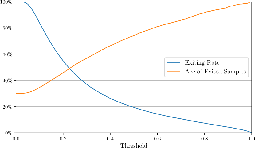
Figure 3: Accuracy of predictions at the $1^{st}$ exit (located at $1^{st}$ skip connection’s output) of ResNet-50 for ImageNet. As the threshold increases, fewer samples exit at this position while the accuracy is rising.

V Configuration Searching

The configuration of deployed exits should be optimized to achieve specific performance or complexity targets.

However, the search space is vast as the number of possible exit combinations are $\prod_{n=1}^{N-1}(K_{n}+1)$, and each of them has thresholds. It is extremely difficult to go through every possibility to find the optimal configuration. Therefore, one contribution of this work is to provide search algorithms for identifying which exit configuration should be used under a specific constraint. Our technique also allows changing the constraints in real time to achieve adjustable trade-offs.

V-A Performance metrics

Configuration searching should consider two sets of goals: Model performance and Complexity. In this work, we equate them to the overall model accuracy and the number of MAC operations relative to the original model.

V-A1 Relative Overall Accuracy

The overall accuracy is computed by aggregating predictions from all exits. Assume that we are working on a model with $N$ segments and a dataset of $M$ samples. By executing the inference algorithm on the dataset, for every sample, all exit outputs in a configuration $G=\{\boldsymbol{k},\boldsymbol{t}\}$ is recorded as $\tilde{\boldsymbol{y}}_{n,k_{n}}$ and the predicted probability of $i^{th}$ class for $m^{th}$ sample is represented as $\tilde{\boldsymbol{y}}^{(m,i)}_{n,k_{n}}$. We then define $W_{n}(\boldsymbol{k},\boldsymbol{t})$ as indices of samples that have confidence higher than the corresponding threshold $t_{n}$ at the $n^{th}$ exit. $U_{n}(\boldsymbol{k},\boldsymbol{t})$ is $W_{n}(\boldsymbol{k},\boldsymbol{t})$ excluding any previously exited samples, i.e., indices of samples which are exited at $n^{th}$ position. $V_{n}(\boldsymbol{k},\boldsymbol{t})$ is a subset of $U_{n}(\boldsymbol{k},\boldsymbol{t})$ where every prediction is correct. These variables are defined mathematically in Eqn. (4), (5) and (6).

$$W_{n}(\boldsymbol{k},\boldsymbol{t}) =\{m:\mathop{max}_{i}(\tilde{\boldsymbol{y}}^{(m,i)}_{n,k_{n}})\geq t_{n}\}$$ (4)

$$U_{n}(\boldsymbol{k},\boldsymbol{t}) =W_{n}(\boldsymbol{k},\boldsymbol{t})\setminus{\textstyle\bigcup_{n^{\prime}=1}^{n-1}W_{n^{\prime}}}(\boldsymbol{k},\boldsymbol{t})$$ (5)

$$V_{n}(\boldsymbol{k}) =\{m:\mathop{argmax}_{i}(\tilde{\boldsymbol{y}}^{(m,i)}_{n,k_{n}})=\boldsymbol{y}^{(m,i)}\}$$ (6)

where the maximization in Eqn. (6) are done over all possible classes (indexed by $i$). The number of samples that reach and exit from the $n^{th}$ exit of configuration $G=\{\boldsymbol{k},\boldsymbol{t}\}$ can be counted as $E_{n}(k,t)$, and the number of these that are correct can be counted as $EC_{n}(k,t)$.

$$E_{n}(\boldsymbol{k},\boldsymbol{t}) =\left|U_{n}(\boldsymbol{k},\boldsymbol{t})\right|$$ (7)

$$EC_{n}(\boldsymbol{k},\boldsymbol{t}) =\left|U_{n}(\boldsymbol{k},\boldsymbol{t})\cap V_{n}(\boldsymbol{k})\right|$$ (8)

where $\left|S\right|$ means the cardinality of a set $S$.
Then the accuracy is measured by the corrected predictions over the total, i.e.,

$$A_{n}(\boldsymbol{k},\boldsymbol{t})=\frac{EC_{n}(\boldsymbol{k},\boldsymbol{t})}{E_{n}(\boldsymbol{k},\boldsymbol{t})}$$ (9)

Now we define the overall accuracy as:

$$A(\boldsymbol{k},\boldsymbol{t})=\frac{1}{M\cdot A_{ori}}\sum_{n=1}^{N}\left|E_{n}(\boldsymbol{k},\boldsymbol{t})\right|A_{n}(\boldsymbol{k},\boldsymbol{t})$$ (10)

where $A_{ori}$ is the accuracy of the original model. This is a normalized factor making $A(\boldsymbol{k},\boldsymbol{t})\in[0,1]$.

V-A2 Relative Run-time Complexity

This paper considers the number of MAC operations as a proxy for complexity. Moreover, we normalize the number of MAC operations in a given functional block with respect to the total number of MAC operations in the original network. We define the following normalised complexity measures: 1) Let $\text{S}_{n}$ be the normalized complexity of the $n^{\text{th}}$ segment alone. Accordingly $\sum_{n=1}^{N}\text{S}_{n}=1$. 2) Let $\Delta_{n,k}\geq 0$ be the complexity of the exit function $f_{n,k}$. Note that $\Delta_{n,0}=0$ for all $n$ as this is the “no exit” i.e. exit disabled, option. Then the average run-time complexity of a configuration is defined as:

$$C(\boldsymbol{k},\boldsymbol{t}) =\frac{1}{M}\sum_{n=1}^{N}E_{n}(k_{n},t_{n})\sum_{n^{\prime}=1}^{n}\left(S_{n^{\prime}}+\Delta_{n^{\prime},k_{n^{\prime}}}\right)$$ (11)

V-B Generating configurations

V-B1 Optimization Target

The model compression needs to take both performance and complexity into consideration. Our proposed dynamic compression method is designed to generate a series of configurations with respect to the relative importance of performance and complexity. We summarise both factors with a parameter $\lambda$ into the following target function:

$$f(\boldsymbol{k},\boldsymbol{t},\lambda) \triangleq\lambda\left(1-A(\boldsymbol{k},\boldsymbol{t})\right)+(1-\lambda)C(\boldsymbol{k},\boldsymbol{t})$$ (12)

Where $0\leq\lambda\leq 1$ is a user-controlled parameter to adjust the relative importance of accuracy and complexity, i.e., as $\lambda\rightarrow 1$, then the object becomes system classification error rate $=1-A(G)$ and so a minimization process would maximize the accuracy with no consideration to the complexity cost. Conversely, as $\lambda\rightarrow 0$, solutions with minimal complexity would be found at the cost of accuracy. This function will be used as the target of a minimization algorithm.

V-B2 Searching for configurations

The configuration search problem is a non-differentiable and non-continuous multi-variable optimization problem, making it exceedingly difficult to devise algorithms that directly optimize $f(\boldsymbol{k},\boldsymbol{t},\lambda)$. Thus, we reformulate this problem as a single-variable problem by only allowing modifications to an existing configuration $G={\boldsymbol{k},\boldsymbol{t}}$ at one position. Consequently, the objective function transforms into:

$$f_{\boldsymbol{k},\boldsymbol{t},\lambda,n}(k_{c},t_{c})~{}\triangleq~{} \lambda\left(1-A_{\boldsymbol{k},\boldsymbol{t},n}(k_{c},t_{c})\right)$$ (13)

$$+(1-\lambda)C_{\boldsymbol{k},\boldsymbol{t},n}(k_{c},t_{c})$$

Here, $(k_{c},t_{c})$ denotes the latent action at the $n^{th}$ exiting position. If both $A_{\boldsymbol{k},\boldsymbol{t},n}(k_{c},t_{c})$ and $C_{\boldsymbol{k},\boldsymbol{t},n}(k_{c},t_{c})$ are monotonically increasing, then $f_{\boldsymbol{k},\boldsymbol{t},\lambda,n}(k_{c},t_{c})$ will be convex. When the threshold of any early exit is increased, more samples progress to the next exit, which invariably requires additional computation. Therefore, $C_{\boldsymbol{k},\boldsymbol{t},n}(k_{c},t_{c})$ is monotonically increasing. With regard to accuracy, as noted in Sec.IV-C, an increased threshold initially enhances the accuracy of the current exit. Moreover, samples reaching later exits are classified more accurately provided all exiting networks have a modest scale relative to the backbone, thus making $A_{\boldsymbol{k},\boldsymbol{t},n}(k_{c},t_{c})$ also monotonically increasing. Therefore, as long as later exits consistently require more computation and yield higher accuracy, $f_{\boldsymbol{k},\boldsymbol{t},\lambda,n}(k_{c},t_{c})$ is convex and its convergence is guaranteed.

Once $f_{\boldsymbol{k},\boldsymbol{t},\lambda,n}(k_{c},t_{c})$ can be minimized, we traverse different layers and exit types to ascertain the optimal action. This action is then applied to the existing configuration. This process is repeated until the round limit is reached, or no additional action can enhance the current configuration. This search method is encapsulated in our proposed Iterative Search, as depicted in Algo.2. Although this algorithm employs a greedy approach, which does not guarantee convergence to the optimum, it effectively narrows the search space to an acceptable range.

Input: $\lambda$

Output: Exit configuration, $G=\{\boldsymbol{k},\boldsymbol{t}\}$.

1 Initialize $\boldsymbol{k}$ and $\boldsymbol{t}$ to be $N\times 1$ vectors of zeros, i.e. no exits by default.

2 Initialize cost metric, $f_{min}=f(\boldsymbol{k},\boldsymbol{t},\lambda)$.

3 while $\mathrm{True}$ do

4       $\mathrm{Candidate}\leftarrow\mathrm{None}$

5       for $n=1\rightarrow N$ do

6             for $k_{c}=0\rightarrow K_{n}$ do

7                   $\{t_{c},~{}f_{c}\}\leftarrow\mathop{min}_{t_{c}}f_{\boldsymbol{k},\boldsymbol{t},\lambda,n}(k_{c},t_{c})$

8                   if $f_{c}<f_{min}$ then

9                         $\mathrm{Candidate}\leftarrow\{n,k_{c},t_{c}\}$

10                         $f_{min}\leftarrow f_{c}$

11                  

12            

13      if $\mathrm{Candidate}~{}\text{is not}~{}\mathrm{None}$ then

14             $n,~{}k_{c},~{}t_{c}\leftarrow\mathrm{Candidate}$

15             $t_{n}\leftarrow t_{c}$       $k_{n}\leftarrow k_{c}$

16            

17       else

18             break

19      

Algorithm 2 Iterative Search algorithm

where $\mathop{min}_{t_{c}}f_{\boldsymbol{k},\boldsymbol{t},\lambda,n}(k_{c},t_{c})$ is a bounded minimization algorithm to find a $t_{c}\in(0,1)$ such that the function value is minimized to $f_{c}$.
However, the iterative search algorithm will still be time-consuming when dealing with large datasets. As an alternative, a simpler and more straightforward substitution is proposed, i.e. the single-pass search algorithm. This method involves only one pass from the first to the last segment. In this algorithm, the search process starts with an assumed empty configuration. Then we begin with the first possible exiting position ($n=1$) and add the option to help the configuration achieve the lowest $f_{c}$. With this action taken into use, we then consider the next exit position until $n=N$, i.e., we make a single-pass through all possible positions hence the name. The single-pass algorithm dramatically saves the searching time, and our experiments indicate it do not have a significant impact on results.

Input: $\lambda$

Output: Exit configuration, $G=\{\boldsymbol{k},\boldsymbol{t}\}$.

1 Initialize $\boldsymbol{k}$ and $\boldsymbol{t}$ to be $N\times 1$ vectors of zeros, i.e. no exits.

2 Initialize cost metric, $f_{min}=f(\boldsymbol{k},\boldsymbol{t},\lambda)$.

3 for $n=1\rightarrow N$ do

4       for $k_{c}=0\rightarrow K$ do

5             $\{t_{c},~{}f_{c}\}\leftarrow\mathop{min}_{t_{c}}f_{\boldsymbol{k},\boldsymbol{t},\lambda,n}(k_{c},t_{c})$

6             if $f_{c}<f_{min}$ then

7                   $f_{min}\leftarrow f_{c}$       $t_{n}\leftarrow t_{c}$       $k_{n}\leftarrow k_{c}$

8                  

9            

10      

Algorithm 3 Single-pass search algorithm

V-C Configurations for different targets

The result of the search algorithm is a specific configuration that exhibits a trade-off between complexity and performance, determined by the parameter $\lambda$. This search process can be replicated with diverse values of $\lambda$ to derive additional configurations with varying trade-off characteristics. A device executing the model for inference can store multiple pre-defined configurations and toggle between them at runtime. This capability facilitates dynamic model compression depending on the real-time requirements. The interval between multiple $\lambda$ values can be kept minimal to enable fine-grained performance tuning.

VI Simulation

VI-A Base Model and Dataset

In 2016, He et al. presented ResNet[14], which is a residual learning framework to train very deep networks for computer vision tasks. After that, many studies proved that ResNet and its residual structure have a successful performance on various computer vision tasks. The core element of ResNet is the residual block which consists of two or three cascaded convolutional layers with a shortcut. Many of today’s state-of-the-art deep CNNs still follow this structure. This paper validates the proposed early-exit based algorithm on the original version of ResNet[14] and ConvNextv2[22], but the results are applicable to other deep neural networks as well. ResNet was proposed for image classification based on ImageNet-1k[7] which contains 1.28m training images and 50k validation images with a size of 244x244. This paper simulates three variants of ResNet at different depths (ResNet-34, ResNet-50, and ResNet-152) on ImageNet to demonstrate the effectiveness of the proposed method.

VI-B Model Implementation

The backbone part of our model implementation for the ImageNet dataset follows the repository by PyTorch[23]. We attach exits to the output of each residual block in ResNet. ResNet-34 and ResNet-50 have 16 positions for exits, including the last exit (the head of the original models). There are 50 exit points for ResNet-152 since it has more layers. The main purpose of this work is not to compete on performance; we employ five different types of plain MLP, from small to large, for every position except the last one. These five types are MLPs of 1-layer, 3-layer with 500 neurons in each hidden layer, 3-layer with 1000 neurons, 5-layer with 500 neurons, and 5-layer with 1000 neurons. The search algorithm will select either none or one of the options for each position in a configuration.

VI-B1 Training details

The training of the exits is based on an existing pre-trained model. The backbone network is freezed and only the exits will be trained. The forward propagation will go through the whole model, while the backward propagation works only on each exit. The data augmentation follows the same strategy as ImageNet pre-training, and the optimizer is Adam with a learning rate $lr=3\times 10^{-4}$. The loss function is soft cross entropy as mentioned in Section IV-B.

VI-C Performance Evaluation

In this study, we present an evaluation of performance to substantiate the effectiveness of our proposed method. Figure 4 provides a comparative visualization of the performance and computational requirements between our proposed approach and other methods. Our approach is validated with base models such as ResNet[14] and ConvNextv2[22]. Each point on the depicted curve signifies an available configuration, providing the option for the user to select in real-time.

TABLE II: Required Multiply-Accumulate operations (MACs) when a certain drop in accuracy (ACC) is allowed

[b] Base Model Required MACs when ACC drop¹ $\leq$ 5.0% 2.0% 0.5% ResNet-34 66.0% 73.5% 79.4% ResNet-50 64.1% 70.8% 79.1% ResNet-101 59.9% 67.8% 76.7% ResNet-152 56.7% 65.8% 76.5% ConvNextv2_atto 79.5% 84.8% 90.0% ConvNextv2_femto 80.6% 86.3% 91.0% ConvNextv2_pico 76.1% 82.3% 87.7% ConvNextv2_nano 67.0% 73.6% 81.9% ConvNextv2_tiny 60.0% 67.0% 74.1%

• Relative to the accuracy of base models

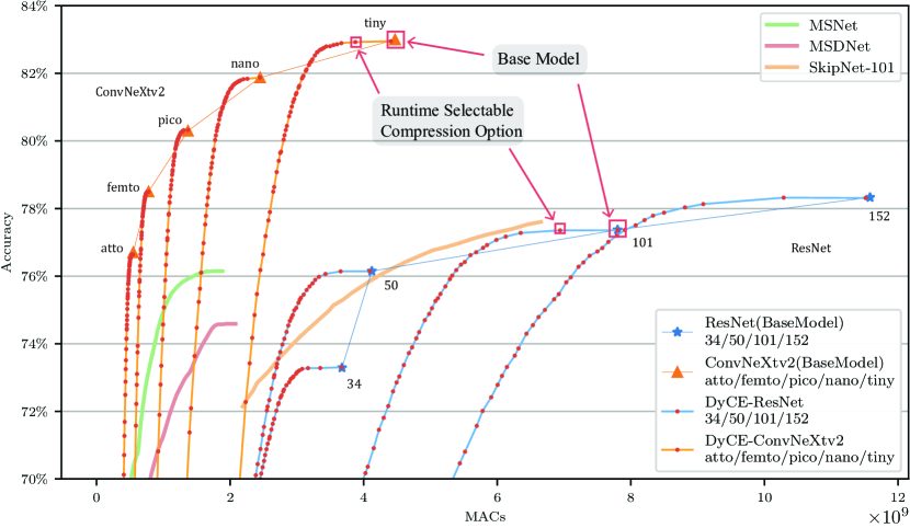
Figure 4: MACs and Accuracy of the proposed method, base models and related work. Original ResNet and ConvNeXtv2 variants are represented as blue stars and orange triangles, the compressed version is denoted by the curve attached to each of them. Three related work is also plotted for reference. These models can not be configured in runtime or adaptive to new base models. However, DyCE can switch to different configurations (denoted by red dots) in runtime and adapt different models such as ResNet and ConvNextv2.

As a compression method, DyCE possesses the capability to conserve computational resources while incurring minimal performance degradation. Table II depicts the experimental results regarding the minimum Multiply-Accumulate operations (MACs) needed to retain specific accuracy levels. Table II depicts the experimental results regarding the minimum Multiply-Accumulate operations (MACs) needed to retain specific accuracy levels. Our proposed system requires only 76.5% to 79.4% of MACs to uphold a comparable accuracy (a diminution of $\leq 0.5\%$) for four variants of ResNet on the ImageNet dataset. As for the ConvNeXtv2 model, both the tiny and nano versions can be compressed by 18.1% and 25.9%, respectively, without significant accuracy degradation. However, the three smaller versions present a more challenging compression scenario, requiring a compromise of over 2% in accuracy for a similar reduction in MACs. For all these models, if a larger decrease in accuracy is permissible, DyCE has the potential to further curtail computational demands by approximately 15% to 20%, albeit with a 5% reduction in accuracy.

Further information is visualized in Figure 4, where we have plotted the DyCE compression curve for each base model. Each dot on the curve denotes a run-time selectable configuration that enables a different trade-off point between complexity and performance. We employed a step size of 0.01 for $\lambda\in[0,1]$ to generate these curves. The density can be augmented to facilitate almost continuous performance tuning.

DyCE exhibits advantages compared with the native architecture scaling, particularly in regions close to the base model. The DyCE curve for ResNet-152 initially surpasses the linear trajectory between ResNet-152 and ResNet-101 but subsequently falls slightly below the point representing ResNet-101. Nevertheless, ResNet-50 augmented with DyCE, consistently outperforms ResNet-34. These findings underscore the potential of DyCE as a beneficial supplement to conventional static model scaling.

Comparative results from other dynamic scaling methods, such as MSDNet, MSNet, and SkipNet-101, are also depicted in Figure 4. These models are task-specific and not runtime configurable, their performance degrade more slowly compared to our plain MLP exits. Given the independence of each exit within DyCE, this challenge can potentially be mitigated by introducing dedicatedly designed exiting networks. Despite the simplicity of the MLPs, DyCE can surpass the efficiency of other methods when suitable base models are chosen. As the proposed framework is decoupled from the base model, it facilitates seamless integration with state-of-the-art models, such as ConvNextv2. The evaluation results of DyCE in conjunction with ConvNextv2 denote a substantial improvement over competing methods. While other techniques generally require model-specific knowledge for designing exits, they may not be easily applicable to the latest models. Considering the rapid evolution of deep learning, the flexibility offered by DyCE is a valuable feature.

VI-D Comparison between Searching Algorithms

We have proposed two search algorithms for generating configurations: the iterative method, which is expected to yield better convergence, and the single-pass method, which offers significantly faster completion. The time complexity of the single-pass algorithm is directly proportional to the number of candidate exits, while the iterative method requires repetitive inspection of every exit, leading to substantially higher complexity. In our experiments, both algorithms have been implemented with GPU acceleration. The single-pass method requires 1.5 minutes to find 100 different configurations for ResNet-50, whereas the iterative method requires 28.9 minutes for completion. The disparity in time taken becomes more pronounced with an increase in the number of exits. For instance, ResNet-152, which has 50 exit positions, requires 4.9 minutes and 215.5 minutes to finish using the two respective methods.

Despite the substantial time investment, as depicted in Fig.5, the iterative method provides a slight edge over the single-pass method. However, considering that configurations only need to be generated once, we recommend utilizing the single-pass method for previewing and debugging purposes and the iterative method for the final generation.

We also compared our proposed algorithms with a baseline method, which selects only one type of exit and applies identical thresholds to all exits. This is the most simplistic approach to make existing early-exit based systems configurable in real time. Figure 5 demonstrates that even when the best exit type is chosen (a 5-layer MLP with 1000 neurons in hidden layers), both of our proposed algorithms exhibit considerable advantages. These results indicate the effectiveness of the search algorithm we propose.

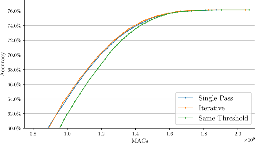
Figure 5: Comparison of three configuration generating methods on ResNet-50.

VI-E Ensemble vs Individual Exits

Figure 6 illustrates the efficacy of utilizing multiple exits collaboratively (represented by the purple line), demonstrating superior performance in comparison to individual exits (represented by the dots in dashed lines). To obtain standalone performance, we emulate a configuration with only one enabled exit and set its threshold to zero, ensuring inference consistently exits at that position. This process is repeated for all potential exits, culminating in the series of dots depicted. As a result, the most optimal type of exit network is “MLP-5x1000”, but the ensemble of exits significantly outperforms any individual types, including the optimal one. As discussed in Section.IV-C, the early exit in more trustable when a threshold is applied. In an exiting configuration, most exits except the final one have thresholds, making most exits perform better than their standalone performance. The systematic average computation is the weighted sum of every exit’s complexity but the accuracy is higher than the sum of exit’s accuracy with the same weight. This observation demonstrates the compression efficiency of early exit groups.

Concurrently, exits at all positions contribute to the overall system performance. The brown line in Fig.6 represents a scenario where the first three positions are disabled. Despite their low accuracy, disabling these exits influences the highest accuracy area, demonstrating that exits at shallow layers have the potential to deal with ‘easy’ samples, and our proposed method can enable them at the right time.

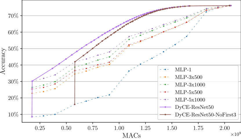
Figure 6: Performance comparison between searched configurations and standalone exits on ResNet-50. MLP-AxB refers to An MLP of A layers with B neurons in all hidden layers.

VII Extensive Design and Usage

This paper demonstrates DyCE with the example of image classification. However, DyCE can be built in alternate ways and deployed to for more applications and more tasks.

VII-A Besides Image Classification

This paper uses the image classification task as an example. However, there should be no barriers to adapting DyCE to other tasks and hierarchical models. DyCE can be applied to any models that are dividable along the depth if we can design checkpoints to generate a candidate prediction in a compatible format as the original output and produce prediction confidence from the output. For example, Transformers[24] for natural language processing is stacked by dividable blocks, and we can also interpret the confidence from the largest value in its output vector. Therefore it should be possible to apply DyCE for Transformer networks.

VII-B Hierarchical multi-tasking

Due to the independence of each checkpoint, this system can be modified to assign different tasks to each checkpoint, such as face recognition, object detection, and image-to-text. These checkpoints with different tasks can be organized in a hierarchical order for specific applications. For the example of the face recognition task, we can assign coarse-grained classifiers to the first few checkpoint positions to determine if there are objects in front of the camera. The next few checkpoints can be fine-grained classifiers to confirm that a human face is in sight. After that, the last few checkpoints can run the regular recognition task. Achieving high performance with a small network is difficult, but it is still possible to get rough answers with limited computation, because the checkpoints attached to the shallow layers can focus on simple but common subtasks. Therefore the majority of the model remains in sleep mode in most cases.

VIII Conclusion

This paper introduces DyCE, a real-time configurable model compression and scaling technique for deep learning models. DyCE simplifies the design process of early-exit-based dynamic compression systems by partitioning the considerations during the design of such systems. It optimizes the cooperation of exits to meet arbitrary compression targets with more efficiency. Furthermore, DyCE introduces a second layer of dynamics to support real-time, fine-grained adjustments to the compression target. This enables applications that employ DyCE to adapt to varying practical demands.

Our experiments validate the effectiveness of the proposed method for image classification tasks employing CNNs. However, the concept of DyCE is not restricted to these domains and could potentially be extended to other models and applications.

References

- [1] M. Dayarathna, Y. Wen, and R. Fan, “Data Center Energy Consumption Modeling: A Survey,” IEEE Communications Surveys & Tutorials, vol. 18, no. 1, pp. 732–794, 2016, conference Name: IEEE Communications Surveys & Tutorials.
- [2] B. Wu, Y. Wang, P. Zhang, Y. Tian, P. Vajda, and K. Keutzer, “Mixed Precision Quantization of ConvNets via Differentiable Neural Architecture Search,” arXiv:1812.00090 [cs], 2018. [Online]. Available: http://arxiv.org/abs/1812.00090
- [3] D. Blalock, J. J. Gonzalez Ortiz, J. Frankle, and J. Guttag, “What is the State of Neural Network Pruning?” Proceedings of Machine Learning and Systems, vol. 2, pp. 129–146, Mar. 2020. [Online]. Available: https://proceedings.mlsys.org/paper/2020/hash/d2ddea18f00665ce8623e36bd4e3c7c5-Abstract.html
- [4] M. Lin, L. Cao, S. Li, Q. Ye, Y. Tian, J. Liu, Q. Tian, and R. Ji, “Filter Sketch for Network Pruning,” IEEE Transactions on Neural Networks and Learning Systems, pp. 1–10, 2021.
- [5] S. Teerapittayanon, B. McDanel, and H. Kung, “BranchyNet: Fast inference via early exiting from deep neural networks,” in 2016 23rd International Conference on Pattern Recognition (ICPR), 2016, pp. 2464–2469.
- [6] Y. Kaya, S. Hong, and T. Dumitras, “Shallow-Deep Networks: Understanding and Mitigating Network Overthinking,” in Proceedings of the 36th International Conference on Machine Learning. PMLR, 2019, pp. 3301–3310. [Online]. Available: https://proceedings.mlr.press/v97/kaya19a.html
- [7] O. Russakovsky, J. Deng, H. Su, J. Krause, S. Satheesh, S. Ma, Z. Huang, A. Karpathy, A. Khosla, M. Bernstein, and others, “Imagenet large scale visual recognition challenge,” International journal of computer vision, vol. 115, no. 3, pp. 211–252, 2015, publisher: Springer.
- [8] S. Hong, Y. Kaya, I.-V. Modoranu, and T. Dumitraş, “A Panda? No, It’s a Sloth: Slowdown Attacks on Adaptive Multi-Exit Neural Network Inference,” Feb. 2021, arXiv:2010.02432 [cs]. [Online]. Available: http://arxiv.org/abs/2010.02432
- [9] R. Hang, X. Qian, and Q. Liu, “MSNet: Multi-Resolution Synergistic Networks for Adaptive Inference,” IEEE Transactions on Circuits and Systems for Video Technology, vol. 33, no. 5, pp. 2009–2018, May 2023, conference Name: IEEE Transactions on Circuits and Systems for Video Technology.
- [10] X. Chen, H. Dai, Y. Li, X. Gao, and L. Song, “Learning to Stop While Learning to Predict,” Jun. 2020, arXiv:2006.05082 [cs, stat]. [Online]. Available: http://arxiv.org/abs/2006.05082
- [11] X. Dai, X. Kong, and T. Guo, “EPNet: Learning to Exit with Flexible Multi-Branch Network,” in Proceedings of the 29th ACM International Conference on Information & Knowledge Management, ser. CIKM ’20. New York, NY, USA: Association for Computing Machinery, Oct. 2020, pp. 235–244. [Online]. Available: https://dl.acm.org/doi/10.1145/3340531.3411973
- [12] X. Wang, F. Yu, Z.-Y. Dou, T. Darrell, and J. E. Gonzalez, “SkipNet: Learning Dynamic Routing in Convolutional Networks,” Jul. 2018, arXiv:1711.09485 [cs]. [Online]. Available: http://arxiv.org/abs/1711.09485
- [13] J. Lin, Y. Rao, J. Lu, and J. Zhou, “Runtime Neural Pruning,” in Advances in Neural Information Processing Systems, vol. 30. Curran Associates, Inc., 2017. [Online]. Available: https://papers.nips.cc/paper_files/paper/2017/hash/a51fb975227d6640e4fe47854476d133-Abstract.html
- [14] K. He, X. Zhang, S. Ren, and J. Sun, “Deep residual learning for image recognition,” in Proceedings of the IEEE conference on computer vision and pattern recognition, 2016, pp. 770–778.
- [15] M. Tan and Q. V. Le, “EfficientNet: Rethinking Model Scaling for Convolutional Neural Networks,” in Proceedings of the 36th International Conference on Machine Learning, ICML 2019, 9-15 June 2019, Long Beach, California, USA, ser. Proceedings of Machine Learning Research, K. Chaudhuri and R. Salakhutdinov, Eds., vol. 97. PMLR, 2019, pp. 6105–6114. [Online]. Available: http://proceedings.mlr.press/v97/tan19a.html
- [16] D. D. Lin, S. S. Talathi, and V. S. Annapureddy, “Fixed Point Quantization of Deep Convolutional Networks,” in Proceedings of the 33nd International Conference on Machine Learning, ICML 2016, New York City, NY, USA, June 19-24, 2016, ser. JMLR Workshop and Conference Proceedings, M.-F. Balcan and K. Q. Weinberger, Eds., vol. 48. JMLR.org, 2016, pp. 2849–2858. [Online]. Available: http://proceedings.mlr.press/v48/linb16.html
- [17] Y. Han, G. Huang, S. Song, L. Yang, H. Wang, and Y. Wang, “Dynamic Neural Networks: A Survey,” IEEE Transactions on Pattern Analysis and Machine Intelligence, vol. 44, no. 11, pp. 7436–7456, Nov. 2022, conference Name: IEEE Transactions on Pattern Analysis and Machine Intelligence.
- [18] W. Liu, P. Zhou, Z. Zhao, Z. Wang, H. Deng, and Q. Ju, “FastBERT: a Self-distilling BERT with Adaptive Inference Time,” Apr. 2020, arXiv:2004.02178 [cs]. [Online]. Available: http://arxiv.org/abs/2004.02178
- [19] I. Leontiadis, S. Laskaridis, S. I. Venieris, and N. D. Lane, “It’s always personal: Using Early Exits for Efficient On-Device CNN Personalisation,” in Proceedings of the 22nd International Workshop on Mobile Computing Systems and Applications, Feb. 2021, pp. 15–21, arXiv:2102.01393 [cs]. [Online]. Available: http://arxiv.org/abs/2102.01393
- [20] M. W. Gardner and S. R. Dorling, “Artificial neural networks (the multilayer perceptron)—a review of applications in the atmospheric sciences,” Atmospheric Environment, vol. 32, no. 14, pp. 2627–2636, 1998. [Online]. Available: https://www.sciencedirect.com/science/article/pii/S1352231097004470
- [21] G. Hinton, O. Vinyals, and J. Dean, “Distilling the Knowledge in a Neural Network,” arXiv:1503.02531 [cs, stat], Mar. 2015, arXiv: 1503.02531. [Online]. Available: http://arxiv.org/abs/1503.02531
- [22] S. Woo, S. Debnath, R. Hu, X. Chen, Z. Liu, I. S. Kweon, and S. Xie, “ConvNeXt V2: Co-designing and Scaling ConvNets with Masked Autoencoders,” Jan. 2023, arXiv:2301.00808 [cs]. [Online]. Available: http://arxiv.org/abs/2301.00808
- [23] P. Team, “ResNet - PyTorch.” [Online]. Available: https://pytorch.org/hub/pytorch_vision_resnet
- [24] A. Vaswani, N. Shazeer, N. Parmar, J. Uszkoreit, L. Jones, A. N. Gomez, L. Kaiser, and I. Polosukhin, “Attention is All you Need,” in Advances in Neural Information Processing Systems, vol. 30. Curran Associates, Inc., 2017. [Online]. Available: https://papers.nips.cc/paper/2017/hash/3f5ee243547dee91fbd053c1c4a845aa-Abstract.html