1 Introduction
In 1843, Hamilton extended the complex number field to quaternions which is a four dimensional division algebra over the real number field . It is well-known that Hamilton quaternions have successful applications in signal and color image processing (e.g., [5]). To keep the commutativity of usual number systems, in 1892, Segre ([18]) discovered the following extension:
|
|
|
Clearly, . is a four dimensional commutative algebra over and contains zero divisors. It is called Segre biquaternion ([14]), commutative quaternion ([9, 12, 13]) or reduced biquaternion ([13, 17]). In this paper, we call it “reduced biquaternion” ( or RB for short).
Reduced biquaternion has numerous applications in many areas. In signal and
color image processing, Pei et al. ([12, 13]) show that the operations of the discrete reduced biquaternion Fourier transforms and their corresponding convolutions and correlations are much simpler than the existing implementations of the Hamilton quaternions, and many questions can be performed simultaneously by . They use reduced biquaternion matrices to represent the color images, then compress the images by the SVDs of reduced biquaternion matrices (RBSVDs). For comparison, they found that the calculating of RBSVD is faster than SVD of a quaternion matrix (QSVD), and the reconstruction quality is also better than one by QSVD method.
By adopting the special structure of a real representation of a reduced
biquaternion matrix, Ding et al. [4] investigated the least-squares special minimal norm solutions to RB matrix equation and applied the least-squares minimal norm RB solution to the color image restoration.
A tensor can be regarded as a multidimensional array.
People use tensors to collect and employ multi-way data.
Tensors and tensor decompositions ([3, 6, 7, 8, 10, 15, 19]) have been applied in many areas such as signal processing,
computer science, data mining, neuroscience, and more.
Studying tensor rank decomposition may go back to the 1960s: the CANDECOMP/PARAFAC (CP) decomposition ([3]) and the Tucker decomposition ([19]).
In [6], Kilmer and Martin defined a closed multiplication operation (called t-product) for two real tensors, and considered some important theoretical properties and practical tensor approximation problems.
Qin et al. [15] defined a tensor product for third-order quaternion tensors and discussed the Qt-SVD of a third-order quaternion tensor with applications in color video.
Motivated by the works mentioned above, in particular, the applications of reduced biquaternion matrices in color image processing, we introduce the applications of reduced biquaternion tensors in color video compression.
This paper is organized as follows. We first introduce some operations over reduced biquaternion tensors, and then we define the Ht-product and explore some important properties of third-order RB tensors in Section 2.
In Section 3, we investigate the Ht-SVD of a third-order RB tensor and develop a method to compute it.
Two theoretical applications of Ht-SVD are given in Sections 4 and 5. That is, in Section 4, the Moore-Penrose inverse of a third-order RB tensor is defined and some properties including algebraic expression derived by the Ht-SVD are discussed. In Section 5, we consider the general/Hertmian/least-squares solutions to reduced biquaternion tensor equation .
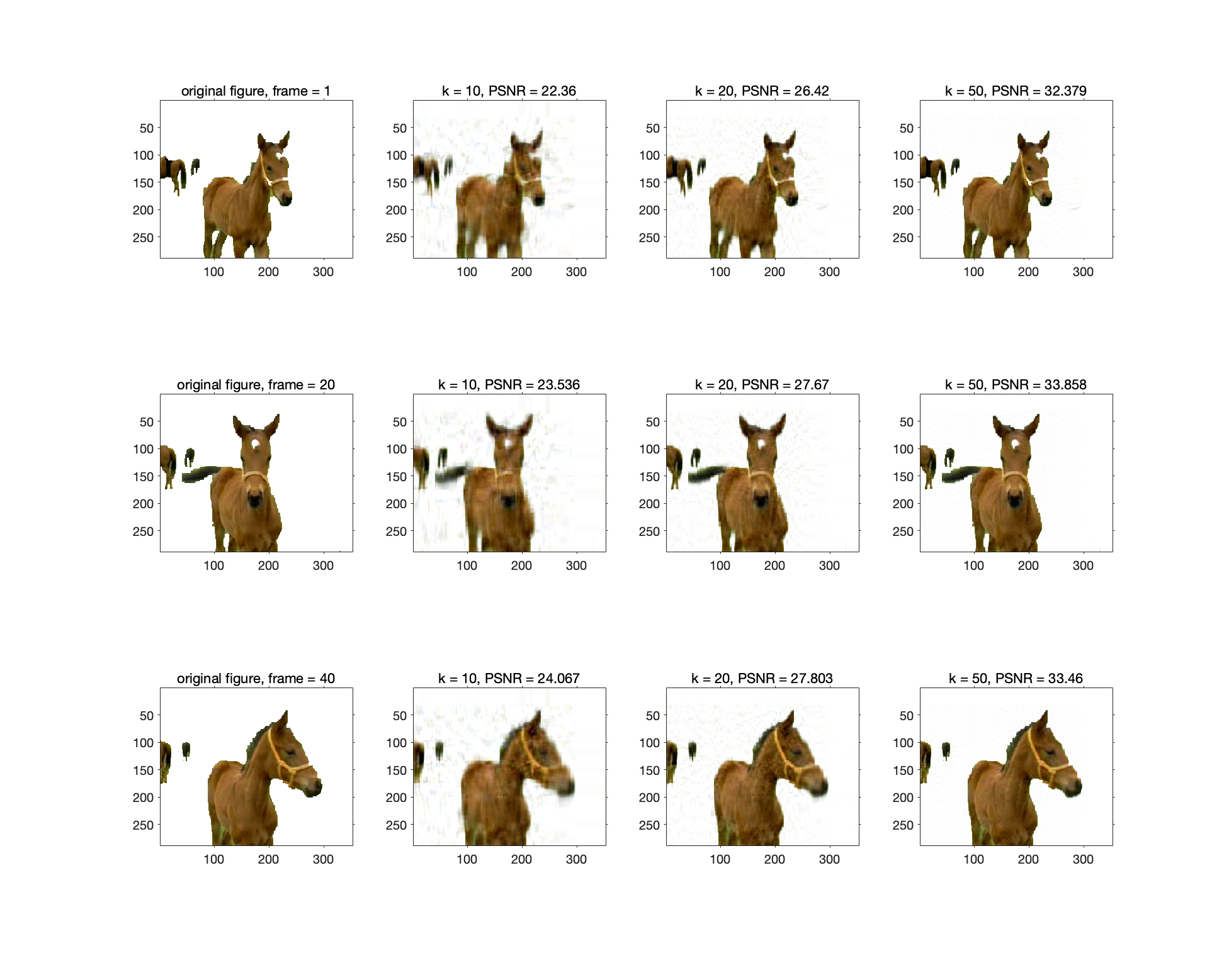
Finally, in Section 6, we apply this Ht-SVD in color video compression. The experimental data shows that our method has an excellent performance comparing with another method.
2 The Ht-product of third-order tensors over
Throughout this paper, Euler script letters are used to refer to tensors, while the capital letters represent matrices.
The notations and represent the set of all the matrices of dimension and all the third-order tensors of dimension over algebra respectively. For a third-order tensor , we denote the th horizontal, the th lateral and the th frontal slice by and respectively. For simplicity, let represent the th frontal slice .
Recall that an element can be expressed as , where
, and . Clearly, and
are two special reduced biquaternions satisfying and ([13]).
For any matrix , we can write it in two forms, that is, with . Then its conjugate transpose is given by . Moreover,
is said to be Hermitian (resp. unitary) if and only if (resp. ).
Furthermore, if we rewrite a as , where and are complex matrices,
then the conjugate transpose of is .
Thus for any ,
, and we can use it to prove that
.
The block circulant matrix generated by a third-order tensor ’s
frontal slices is given as
|
|
|
We will use Vec operator to convert a tensors into a block matrix :
|
|
|
and the inverse operation Fold to take the block matrix back to a tensor:
|
|
|
Moreover, we use the frontal slices of to define a block diagonal matrix as following:
|
|
|
(1) |
Note that by using the normalized Discrete Fourier transformation (DFT) matrix, a complex circulant matrix can be diagonalized ([6], [15]). Suppose is a third-order complex tensor.
Then
|
|
|
(2) |
where denotes the Kronecker product, () are the frontal slices of the tensor which is the result of DFT of along the third mode,
is unitary and .
Definition 2.1
The DFT of along the third mode is a tensor satisfying
|
|
|
We can verify the relation between and as follows.
|
|
|
(3) |
Now we extend -product of two third-order real tensors defined in [6] to reduced biquaternions.
Definition 2.2
(Ht-product)
Let and . Then -product of and is defined as
|
|
|
where ,
The addition and scalar multiplication rules of tensors over are defined in a usual way.
Theorem 2.3
Let and with the corresponding DFTs and .
Then if and only if
Proof.
Since is the DFT of along the third mode,
it follows from (3) and that
|
|
|
|
|
|
|
|
which implies
|
|
|
(4) |
By Definition 2.2
and identities (2) and (3), we have
|
|
|
|
|
|
|
|
|
|
|
|
|
|
|
|
Thus
|
|
|
Combing with equation (4) yields
.
Therefore,
|
|
|
According to the above result, we can give an equivalent definition of the Ht-product of two third-order reduced biquaternion tensors.
Definition 2.4
Let and . The -product of and is defined as
|
|
|
where is an vector with all the entries equal to 1.
This Ht-product obeys some usual algebraic operation laws, such as the associative law and the distributive law.
Proposition 2.5
Let and . Then
|
|
|
Proof.
By Definition 2.4, we have
|
|
|
|
|
|
|
|
and
|
|
|
|
|
|
|
|
Notice that and are matrices over . Hence the associative law holds, and thus the result holds.
In a similar way as in Proposition 2.5, we have the following distributive laws. For brevity, we omit the proofs.
Proposition 2.6
Let and . Then
|
|
|
|
|
|
Suppose . Using the method in [15], we calculate the conjugate transpose of
as follows: first conjugately transposing each frontal slice of first, and reversing the order of conjugately transposed frontal slices through next.
Definition 2.7
The conjugate transpose of with is defined as with .
It is not difficult to verify that and for .
Definition 2.8
The identity tensor (simply denoted by ) is the tensor in which the first frontal slice is and the other slice matrices are zero.
We can obtain that , and
Definition 2.9
A tensor is called invertible if there is a tensor such that
and
.
By using Proposition 2.5 and the fact , we have the following result.
Proposition 2.10
The inverse of a Segre quaternion tensor is unique if it exists, denoted by .
Definition 2.11
Let . is called idempotent if
;
is called unitary (resp. Hermitian) if
Lemma 2.12
Let . Then
Proof.
It is easy to see that for
According to the equality (2), we have
|
|
|
|
|
|
|
|
|
|
|
|
The above result over can be extended to as follows.
Proposition 2.13
Let . Then
Proof.
Since is the DFT of and , it follows from (3) that
|
|
|
|
|
|
|
|
|
|
|
|
which is equivalent to
|
|
|
(5) |
Similarly, we have Its conjugate transpose is Combing with equality (5) and Lemma 2.12, we have
Corollary 2.14
is Hermitian (resp. unitary) if and only if is Hermitian (resp. unitary).
Proof.
By Definition 2.8,
it is clear that
Then, by Theorem 2.3 and Proposition 2.13, the result follows.
Proposition 2.15
Given and , we have
Proof.
From Theorem 2.3 and Proposition 2.13, we only need to show
|
|
|
In fact, this equality holds for matrices and over .
3 The Ht-SVD of third-order tensors over
The SVD of a matrix over has been discussed in some papers (see, e.g., [13]).
Let . If
and
then the SVD of is
|
|
|
(6) |
where and are unitary matrices, is diagonal but not a real matrix in general.
Recall that a tensor is called -diagonal if each frontal slice is diagonal ([6]).
Next, we propose the Ht-SVD
of a reduced biquaternion tensor.
Theorem 3.1
(Ht-SVD)
Let . Then there exist unitary tensors and such that
|
|
|
where is -diagonal. Such decomposition is called -SVD of .
Proof.
We first transform into by using DFT along the third mode, and then obtain the block diagonal matrix by (1).
In addition, we consider the SVD of each in with formula (6).
Suppose
Then we have
|
|
|
Setting
|
|
|
and
|
|
|
we have
|
|
|
(7) |
in which and are unitary matrices,
and is a block diagonal matrix with elements being diagonal matrices in general.
Next, we construct reduced biquaternion tensors and as follows:
|
|
|
|
|
|
|
|
|
Observing that
That is, are the DFT of tensors , respectively.
Thus by applying Theorem 2.3 and Proposition 2.13 , we infer from the equation (7) that
|
|
|
Obviously, is -diagonal. And according to Corollary 2.14, we know that , are our required unitary tensors.
4 The MP inverses of reduced biquaternion tensors
We refer the readers to [1] for Moore-Penrose (MP) inverses. In this section, as an application of Ht-SVD of a RB tensor, we define the MP inverse for a RB tensor and find a formula for the MP inverse
by using Theorem 3.1. Moreover, we explore some theoretical properties of the MP inverse of RB tensors.
For a given matrix , its MP inverse is the unique matrix (denoted as ) satisfying
|
|
|
According to the properties of reduced biquaternion matrices, we can easily derive the MP inverse of a reduced biquaternion matrix as follows.
Theorem 4.1
Let where . The MP inverse of is
Now, we introduce the definition of the MP inverse of a third-order Segre quaternion tensor.
Definition 4.2
Let .
If there exists satisfying:
-
(i)
-
(ii)
-
(iii)
-
(iv)
then is said to be an MP inverse of , denoted by
For each reduced biquaternion tensor, the following theorem shows that it has a unique MP inverse.
Theorem 4.3
Let and its Ht-SVD be
where are unitary and
is f-diagonal.
Then has a unique MP inverse
|
|
|
(8) |
where .
Proof.
From Theorem 2.3, Proposition 2.5, Proposition 2.15 and Definition 4.1, it is not difficult to verify that and the expression of given in (8) satisfies all four conditions in Definition 4.2.
Next, we need to prove the uniqueness of the MP inverse.
Suppose that and are two MP inverses of , respectively. Then
|
|
|
|
|
|
|
|
|
|
|
|
|
|
|
|
|
|
|
|
|
|
|
|
|
|
|
|
The proof is completed.
Next, we explore some properties of the MP inverse of a reduced biquaternion tensor .
Proposition 4.4
Let . Then
-
(a)
;
-
(b)
;
-
(c)
and ;
-
(d)
( and are unitary reduced biquaternion tensors );
-
(e)
If is f-diagonal, then is f-diagonal, and . In this case, if each diagonal entry in each frontal slice has an inverse, then ;
-
(f)
;
-
(g)
;
-
(h)
;
-
(i)
and ;
-
(j)
;
-
(k)
;
-
(l)
if ;
-
(m)
and are idempotent;
-
(n)
If is Hermitian and idempotent, then .
Proof. We only prove (b), (c), (d), (l) and (n). In the analogous way, one can obtain the remaining properties.
-
(b)
Using Propositions 2.5 and 2.15, one can obtain that is the MP inverse of by direct calculations.
-
(c)
By (b), Proposition 2.5, Proposition 2.15 and the fact , one can get that is the MP inverse of and is the MP inverse of .
-
(d)
Suppose and . Then we have
|
|
|
|
|
|
|
|
|
and
|
|
|
Hence, by Definition 4.2 we can derive that
-
(l)
It follows from (i) and (j).
-
(n)
If is Hermitian and idempotent, then
and . Thus by Definition 4.2 we have .
In general, . Under some conditions, we have the equality case given as follows.
Proposition 4.5
Let and . Then if one of the following conditions satisfies.
(a) ; (b) ; (c) ; (d) .
Denote
represents zero tensor with all the entries being zero.
Obviously,
Proposition 4.6
Let . Then
-
(a)
and ;
-
(b)
and ;
-
(c)
and ;
-
(d)
and ;
-
(e)
and ;
-
(f)
and .
Proof. By straightforward calculations, one can prove that (a), (b) and (d) hold.
For (c), the first equality follows from
|
|
|
and
|
|
|
In an analogous manner, one can prove the second part.
For (e), it follows immediately from (c), (d) and Proposition 4.4.
For (f), The second part can be proved in a similar way.
5 Reduced biquaternion tensor equation
We first discuss the consistency of RB tensor equation
|
|
|
(9) |
by using the MP inverse demonstrated in Section 4.
The solvability conditions are found and a general expression of the solutions is provided when the solutions exist. Furthermore, we also derive solvability conditions and the general solutions involving Hermicity.
Theorem 5.1
Let and
Then equation (9)
has solutions if and only if .
Furthermore, the general solutions to equation (9)
can be written as
|
|
|
(10) |
with be any reduced biquaternion tensor with compatible size.
Proof.
Assume that is a solution to reduced biquaternion tensor equation (9).
Then by Proposition 2.5 and Proposition 4.6, we have
|
|
|
Conversely, if ,
it is easy to see that
is a solution to equation (9), and so is .
Moreover, each solution of equation (9)
has the form of the equation (10) since
Theorem 5.2
Let . Then equation (9)
has a Hermitian solution if and only if
and
Moreover, if (9) is solvable, then the general Hermitian solutions to the Segre quaternion tensor equation (9)
can be written as
|
|
|
(11) |
where is an arbitrary tensor with appropriate size.
Proof.
If equation (9)
has a Hermitian solution ,
then by Propositions 2.5, 2.15 and Definition 4.2, we obtain
|
|
|
and
On the other hand, assume that
and hold.
Then by applying Propositions 2.5 and 2.15, we get that
|
|
|
is a Hermitian solution to Segre quaternion tensor equation (9).
Next we show that each solution of Segre quaternion tensor equation (9)
should be in the form of (11).
Assume is an arbitrary Hermitian solution to tensor equation (9). Setting yields
|
|
|
|
|
|
|
|
|
|
|
|
|
|
|
|
|
|
|
|
|
|
|
|
|
|
|
|
which implies that each Hermitian solution to Segre quaternion tensor equation (9)
can be represented as (11). Thus, (11) is the general expression of Hermitian
solutions to equation (9).
Next, we deal with the least-squares problem of .
It is well known that
Segre quaternion matrices have the following properties. The equivalent complex matrix of reduced biquaternion matrix ([13]) is
|
|
|
(12) |
Given and , we have and .
For , we define the Frobenius norm of as , and -norm as .
Moreover, it can be verified that
|
|
|
(13) |
|
|
|
where
For a tensor
with , we define its Frobenius norm as
|
|
|
(14) |
|
|
|
(15) |
where
Theorem 5.3
Let Then .
Proof.
By applying identities (3), (14) and as well as the invariant property of Frobenius norm under a unitary transformation for
complex matrices, we have
|
|
|
|
|
|
|
|
|
|
|
|
|
|
|
|
|
|
|
|
|
|
|
|
Therefore, .
Lemma 5.4
([1])
The solutions of least-squares problem of complex equation
are
|
|
|
with be any matrix with appropriate size. Furthermore, is the minimum norm least-squares solution.
Lemma 5.5
Suppose
Denote
Then reduced biquaternion least-squares problem has a solution if and only if the complex least-squares problem has a solution
, where is given by (12).
In addition, if is the minimum norm solution to the complex least-squares problem , then is the minimum norm solution to the least-squares problem over .
Proof.
By equation (13), we have
|
|
|
where and are defined by (12).
Then using the fact
|
|
|
we can see that
and arrive the minima at the same time. With Lemma 5.4,
|
|
|
is the least-squares solution to , in which is arbitrary,
and are the least-squares solutions to
Theorem 5.6
Let and with their DFTs and .
Denote
Then is a solution to the tensor least-squares problem if and only if is a solution to the matrix least-squares problem
Moreover, if X is the minimum norm least-squares solution to ,
then
|
|
|
is the minimum norm least-squares solution to
Proof.
By Theorem 2.3 and Theorem 5.3, we have
|
|
|
Notice that
thus
Therefore, if X
is a least-squares solution to then according to Lemma 5.5 and equation (3),
is a least-squares solution to .