Structured methods for parameter inference and uncertainty quantification for mechanistic models in the life sciences

Abstract

Parameter inference and uncertainty quantification are important steps when relating mathematical models to real-world observations, and when estimating uncertainty in model predictions. However, methods for doing this can be computationally expensive, particularly when the number of unknown model parameters is large. The aim of this study is to develop and test an efficient profile likelihood-based method, which takes advantage of the structure of the mathematical model being used. We do this by identifying specific parameters that affect model output in a known way, such as a linear scaling. We illustrate the method by applying it to three caricature models from different areas of the life sciences: (i) a predator-prey model from ecology; (ii) a compartment-based epidemic model from health sciences; and, (iii) an advection-diffusion-reaction model describing transport of dissolved solutes from environmental science. We show that the new method produces results of comparable accuracy to existing profile likelihood methods, but with substantially fewer evaluations of the forward model. We conclude that our method could provide a much more efficient approach to parameter inference for models where a structure approach is feasible. Code to apply the new method to user-supplied models and data is provided via a publicly accessible repository.

Keywords: environmental modelling; epidemic model; maximum likelihood estimation; optimisation; predator-prey model; profile likelihood.

Introduction

Parameter inference and uncertainty quantification are important whenever we wish to interpret real-world data, or to make predictions of that data using mathematical models. This is especially true for modelling applications in the life sciences where data is often scarce and uncertain. Commonly used methods include tools from both frequentist (e.g. maximum likelihood estimation and profile likelihood) [1, 2] and Bayesian statistics (e.g. Markov chain Monte Carlo methods and approximate Bayesian computation) [3, 4, 5]. These methods can be computationally expensive, particularly for mathematical models with many unknown parameters, resulting in a high-dimensional search space. This has led to a significant body of literature concerned with improving the efficiency of parameter inference methods.

In 2014, Hines et al. [6] reviewed the application of Bayesian Markov chain Monte Carlo (MCMC) sampling methods for parameter estimation and parameter identifiability for a range of ordinary differential equation (ODE)-based models of chemical and biochemical networks. Their results indicated that parameter non-identifiability can be detected through MCMC chains failing to converge. Similar observations were made by Siekmann et al. [7] for a range of continuous-time Markov chain models used in the study of cardiac electrophysiology. In 2020, Simpson et al. [8] compared MCMC sampling with a profile likelihood-based method for parameter inference and parameter identifiability for a range of nonlinear partial differential equation (PDE)-based models used to interrogate cell biology experiments. The authors studied identifiable and non-identifiable problems and found that, while both the MCMC and profile likelihood-based approaches gave similar results for identifiable models, only the profile likelihood approach provided mechanistic insight for non-identifiable problems. They also found that profile likelihood was approximately an order of magnitude faster to implement than MCMC sampling, regardless of whether the problem was identifiable or not. The speed-up in computation is a consequence of the fact that it is often faster to use numerical optimisation methods compared to sampling methods. Raue et al. [9] suggested the sequential use of profile likelihood to constrain prior distributions before applying MCMC sampling in the face of non-identifiability.

While profile likelihood has long been used to assess parameter identifiability and parameter estimation [10, 11, 12, 13, 14], Simpson and Maclaren [15] recently presented a profile likelihood-based workflow covering identifiability, estimation and prediction. The workflow uses computationally efficient optimisation-based methods to estimate the maximum likelihood, and then explores the curvature of the likelihood through a series of univariate profile likelihood functions that target one parameter at a time. This workflow then propagates uncertainty in parameter estimates into model predictions to provide insight into how variability in data leads to uncertainty in model predictions. While the initial presentation of the profile likelihood-based workflow focused on deterministic ODE and PDE models, the same ideas can be applied to stochastic models whenever a surrogate likelihood function is available [1].

For many mathematical modelling applications, there is little alternative than to either assume a fixed value for a particular parameter, or include it as a target for inference. However, in some cases, there may be parameters whose values are unknown, but whose effect on the model solution is known to be a simple linear scaling or some other known transformation, as we will demonstrate later. In such cases, finding the optimal (likelihood-maximising) values of these parameters is trivial if the other model parameters are known. However, typically there will be other model parameters that are unknown. Performing standard inference procedures on the full set of unknown parameters is inefficient as it fails to make use the simple scaling relationship associated with some of the parameters.

As a motivating example, [16] described an epidemiological model that was fitted to data in real-time and used to provide policy advice during the Covid-19 pandemic. The model consisted of a system of several thousand ODEs, and model fitting and uncertainty quantification was done using an approximate Bayesian computation method targeting 11 unknown parameters. This resulted in a computationally expensive problem with a high-dimensional parameter space. Two of the fitted parameters were multiplicative factors on the proportion of model infections that led to hospitalisation and death respectively in each age group and susceptibility class. Adjusting either or both of these parameters while holding the other parameters fixed would linearly scale the time series for expected daily hospital admissions and deaths output by the model. Thus, for a given combination of the other nine fitted parameters, it should be possible to find the optimal values for these two parameters without a costly re-evaluation of the full model.

Here, we propose an new approach, which we term structured inference, that exploits the known scaling relationship between certain parameters and the model solution. This approach recasts an $N$-dimensional optimisation problem as a nested pair of lower-dimensional problems, effectively reducing the dimensionality of the search space. We illustrate our method using canonical toy models representing three cases studies drawn from different areas of the life and physical sciences: ecological species interactions; epidemiological dynamics; and pollutant transport and deposition. In each case study, we use the model structure to identify parameters that have a known scaling effect on model output. We then show that implementing a structured inference approach results in solutions with very similar accuracy, but substantially fewer calls to the forward model solver. This suggests that our method could potentially offer significant reduction in computation time when applied to more complex models, which are computationally expensive to solve. Alongside this article, we provide fully documented code for implementing our method, with instructions for how it can be applied to user-supplied models and data.

Methods

Unstructured and structured inference

Suppose a model has $N$ unknown parameters denoted $\theta$. We assume that a likelihood function $L(x,\theta)$ is available for the model for given observed data $x$. A standard approach to parameter inference is to perform maximum likelihood in the $N$-dimensional parameter space. The maximum likelihood estimate $\theta_{\mathrm{MLE}}$ for the parameters is the solution of the optimisation problem

$$\theta_{\mathrm{MLE}}=\mathrm{argmax}_{\theta}L(x,\theta).$$ (1)

When solving this problem numerically, each call to the objective function with a given combination of parameters $\theta$ typically requires calculation of the model solution, denoted $y(\theta)$, in order to calculate the likelihood. This solution could involve solving systems of ODEs or PDEs, depending on the modelling context, using either approximate or exact methods. We refer to this as the ‘basic method’.

In this article, we propose and test a modification to this method. Our modified method can be applied to models where the vector of parameters $\theta$ can be partitioned into $\theta=[\theta_{\mathrm{outer}},\theta_{\mathrm{inner}}]$ such that there is a known relationship between the model solutions $y(\theta_{\mathrm{outer}},\theta_{\mathrm{inner}})$ for parameters with the same value of $\theta_{\mathrm{outer}}$ but different values of $\theta_{\mathrm{inner}}$. This relationship can be expressed in the form of a transformation:

$$y(\theta_{\mathrm{outer}},\theta_{\mathrm{inner}})=F\left(y(\theta_{\mathrm{outer}},\theta_{\mathrm{inner}}^{\mathrm{ref}})\right)$$ (2)

for some known function $F$, which we assume is relatively cheap to compute compared to solving the full forward model for $y(\theta)$. The simplest example is where the model solution is directly proportional $\theta_{\mathrm{inner}}$, in which case this transformation is a simple linear scaling:

$$y(\theta_{\mathrm{outer}},\theta_{\mathrm{inner}})=\frac{\theta_{\mathrm{inner}}}{\theta_{\mathrm{inner}}^{\mathrm{ref}}}y(\theta_{\mathrm{outer}},\theta_{\mathrm{inner}}^{\mathrm{ref}}).$$ (3)

This type of scaling relationship enables a more efficient approach to maximum likelihood estimation because, for fixed $\theta_{\mathrm{outer}}$, the optimal value of $\theta_{\mathrm{inner}}$ may be calculated with only a single run of the forward model. Thus the $N$-dimensional optimisation problem in Eq. (1) may be replaced by a nested pair of lower-dimensional problems:

$$\theta_{\mathrm{outer},\mathrm{MLE}} = \mathrm{argmax}_{\theta_{\mathrm{outer}}}L(x,\theta_{\mathrm{outer}},\theta^{*}_{\mathrm{inner}}),$$ (4)

$$\textrm{where }\qquad\theta^{*}_{\mathrm{inner}} = \mathrm{argmax}_{\theta_{\mathrm{inner}}}L(x,\theta_{\mathrm{outer}},\theta_{\mathrm{inner}}).$$ (5)

To solve the inner optimisation problem in Eq. (5), the full forward model only needs to be run once, for some defined reference value of $\theta_{\mathrm{inner}}=\theta_{\mathrm{inner}}^{\mathrm{ref}}$. The model solution $y^{\mathrm{ref}}=y(\theta_{\mathrm{outer}},\theta_{\mathrm{inner}}^{\mathrm{ref}})$ for this reference value of $\theta_{\mathrm{inner}}$ can then be transformed via Eq. (2) to find the model solution $y(\theta_{\mathrm{outer}},\theta_{\mathrm{inner}})$ for any value of $\theta_{\mathrm{inner}}$. We refer to this as the ‘structured method’ (see Figure 1 for a schematic illustration of the basic and structured methods).

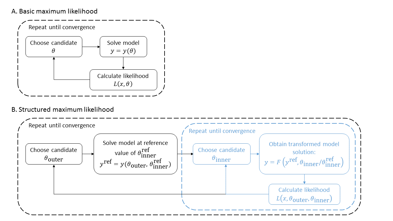
Figure 1: Schematic illustration of: (A) the basic maximum likelihood method and (B) the structured maximum likelihood method. The basic method is an $N$-dimensional optimisation problem for $\theta$. The structured method nests a $k$-dimensional inner optimisation problem for $\theta_{\mathrm{inner}}$ (blue) within an $(N-k)$-dimensional outer optimisation problem for $\theta_{\mathrm{outer}}$ (black). The inner optimisation problem can be solved numerically without rerunning the forward model to find $y$. Candidate values for parameters will typically be chosen using a standard optimisation algorithm.

In this work, given a log-likelihood function, $L(x,\theta)$, we then re-scale to form a normalised log-likelihood $\hat{L}(x,\theta)=L(x,\theta)-L(x,\theta_{\textrm{MLE}})$, where $\theta_{\textrm{MLE}}$ is the MLE so that $\hat{L}(x,\theta_{\textrm{MLE}})=0$. Profile likelihoods are constructed by partitioning the full parameter $\theta$ into interest parameters $\psi$, and nuisance parameters $\omega$, such that $\theta=(\psi,\omega)$ [17]. In this work we construct a series of univariate profiles by specifying the interest parameter to be a single parameter of interest in $\theta_{\mathrm{outer}}$, and the nuisance parameters are the remaining parameters in $\theta_{\mathrm{outer}}$. For a fixed set of data $x$, the profile log-likelihood for the interest parameter $\psi$ given the partition $(\psi,\omega)$ is

$$\hat{L}_{p}(\psi,x)=\sup_{\omega\mid\psi}\hat{L}(\psi,\omega,x),$$ (6)

which implicitly defines a function $\omega^{*}(\psi)$ for optimal values of the nuisance parameters as a function of the target parameters for the given dataset. For univariate parameters this is simply a function of one variable. For identifiable parameters these profile likelihoods will contain a single peak at the MLE.

The degree of curvature of the log-likelihood function is related to inferential precision [17]. Since, in general, univariate profiles for identifiable parameters involve a single peak at the MLE, one way to quantify the degree of curvature of the log-likelihood function is to form asymptotic confidence intervals (CIs) by finding the interval where $\hat{L}_{p}\geq-\Delta_{q,n}/2$, where $\Delta_{q,n}$ denotes the $q$th quantile of the $\chi^{2}$ distribution with $n$ degrees of freedom [18]. For univariate profiles, $n=1$. In this study we identify the interval in the interest parameter $\psi$ where $\hat{L}_{p}\geq-\Delta_{0.95,1}/2=-1.92$, which identifies the 95% CI.

Case studies

Predator–prey model: Ecology

Our first case study is a simple toy model for a prey species $R$ and predator species $P$, assuming a logistic growth for the prey and a type-II functional response (i.e. saturating at high prey density) for the predation term:

$$\frac{dR}{dt} = rx\left(1-\frac{R}{K}\right)-\frac{aRP}{R+b},$$ (7)

$$\frac{dP}{dt} = \frac{aRP}{R+b}-\mu P.$$ (8)

This is a type of Rosenzweig-MacArthur model [19], which is a generalisation of the classical Lotka-Volterra predator-prey model [20, 21].

We suppose that some fixed fraction $p_{\mathrm{obs}}$ of the prey and the predator populations is observed on average at each time point $t$, and observed data $\hat{X}_{t}$ are Poisson distributed:

$$\hat{X}_{1,t} \sim \mathrm{Poisson}(y_{1,t}),$$ (9)

$$\hat{X}_{2,t} \sim \mathrm{Poisson}(y_{2,t}),$$ (10)

where $y_{1,t}=p_{\mathrm{obs}}R(t)$ and $y_{2,t}=p_{\mathrm{obs}}P(t)$ are the expected number of prey and predators observed respectively. For illustrative purposes, we assume the initial conditions and the parameters $K$ and $b$ are known (e.g. from information on the environmental conditions and average prey handling time), and perform inference on the parameter set $\theta=\left(r,a,\mu,p_{\mathrm{obs}}\right)$.

For the structured inference method, we set $\theta_{\mathrm{inner}}=p_{\mathrm{obs}}$, noting that if ${\bf y}_{\mathrm{ref}}$ is the model solution with $\theta_{\mathrm{outer}}=\theta_{\mathrm{outer}}^{\mathrm{ref}}$ and $p_{\mathrm{obs}}=1$, then the solution for a arbitrary value of $p_{\mathrm{obs}}\in[0,1]$ is simply ${\bf y}=p_{\mathrm{obs}}{\bf y}_{\mathrm{ref}}$. Thus, under the structured method, the ordinary differential equation model (7)–(8) only ever needs to be solved with $p_{\mathrm{obs}}=1$. When evaluation of the model likelihood requires the expected value ${\bf y}$ of observed data for any other value of $p_{\mathrm{obs}}$, this is obtained via this simple linear scaling.

SEIR model: Epidemiology

Our second case study is a SEIR compartment model for an epidemic in a closed population of size $N$ [22]. We assume that the population at time $t$ is divided into compartments representing the number of people who are susceptible ($S$), exposed ($E$), infectious ($I$), and recovered ($R$). To model waning immunity, we subdivide the recovered compartment into two compartments $R_{1}$ and $R_{2}$ and assume that individuals transition from $R_{1}$ to $R_{2}$ and subsequently back to $S$. This is described by the following system of ordinary differential equations:

$$\frac{dS}{dt} = -\lambda S+2wR_{2},$$ (11)

$$\frac{dE}{dt} = \lambda S-\gamma E,$$ (12)

$$\frac{dI}{dt} = \gamma E-\mu I,$$ (13)

$$\frac{dR_{1}}{dt} = \mu I-2wR_{1},$$ (14)

$$\frac{dR_{2}}{dt} = 2w(R_{1}-R_{2}),$$ (15)

where $\gamma$, $\mu$ and $w$ are transition rates representing the reciprocal of the mean latent period, infectious period and immune period respectively, and $\lambda$ is the force of infection defined as

$$\lambda(t)=\frac{R_{0}\mu I(t)}{N},$$ (16)

where $R_{0}$ is the basic reproduction number. The model is initialised with a specified number of exposed individuals by setting $E(0)=E_{0}$, $S(0)=N-E_{0}$ and all other variables equal to zero.

We assume that, on average, a fixed proportion $p_{\mathrm{obs}}$ of infections are observed. This could represent epidemiological surveillance data, for example the number of notified cases under the assumption that surveillance effort is steady over time. Alternatively it could represent a particular clinical outcome, such as hospital admission. Unknown case ascertainment or uncertain clinical severity are common, particularly for new or emerging infectious diseases. Hence, joint inference of this parameter with parameters of the SEIR model, in situations where these are identifiable, is an important task in outbreak modelling [16, 23, 24].

Observations are not typically recorded instantaneously at the time of infection, so we assume there is an average time lag of $1/\alpha$ from the time an individual becomes infectious to the time they are observed. These assumptions are modelled via the differential equations

$$\frac{dC_{1}}{dt} = p_{\mathrm{obs}}\gamma E-\alpha C_{1},$$ (17)

$$\frac{dC_{2}}{dt} = \alpha C_{1}.$$ (18)

Here, $C_{1}$ represents the number of infected individuals who will be observed but have not yet been observed, and $C_{2}$ is the cumulative number of observed infections. The expected number of observations per day at time $t$ is denoted $y_{t}$ and is equal to $\alpha C_{1}$.

We assume that the number of observed cases $\hat{X}_{t}$ on day $t$ is drawn from a negative binomial distribution with mean $y_{t}$ and dispersion factor $k$:

$$\hat{X_{t}}\sim\textrm{NegBin}(y_{t},k).$$

We assume that the initial conditions and the transition rates $\gamma$, $\mu$ and $\alpha$ are known (e.g. from independent epidemiological data on the average latent period and infectious period), and perform inference on the parameter set $\theta=\left(R_{0},w,p_{\mathrm{obs}},k\right)$.

Similar to the predator–prey model, we set $\theta_{\mathrm{inner}}=p_{\mathrm{obs}}$, noting that if ${\bf y}_{\mathrm{ref}}$ is the model solution with $\theta_{\mathrm{outer}}=\theta_{\mathrm{outer}}^{\mathrm{ref}}$ and $p_{\mathrm{obs}}=1$, then the solution for a arbitrary value of $p_{\mathrm{obs}}\in[0,1]$ is simply ${\bf y}=p_{\mathrm{obs}}{\bf y}_{\mathrm{ref}}$.

Advection-diffusion-reaction model: Environmental science

In the context of environmental modelling and pollution management, advection-diffusion-reaction models are often used to study how dissolved solutes are spatially distributed over time. Very often the equation for the solute concentration $u(\mathbf{x},t)$ at position $\mathbf{x}$ and time $t$ includes a source term to describe chemical reactions [25]. A common approach is to assume that chemical reactions are fast relative to transport and a linear isotherm model. This gives one of the most common models of reaction-transport.

$$\dfrac{\partial u}{\partial t}=D\nabla^{2}u-v\cdot\nabla u-\dfrac{\partial s}{\partial t},$$ (19)

where $D>0$ is the diffusivity, often called the dispersion coefficient in solute transport modelling literature, $v$ is the advection velocity, and $\partial s/\partial t$ is a sink term that represents a chemical reaction that converts $u(x,t)$ into some immobile product $s(x,t)$. A common form for the sink term is $\partial s/\partial t=fu-gs$, where $f>0$ is the forward reaction rate and $g>0$ is the backward reaction rate. In the limiting case where the chemical reactions occur instantaneously, we have $s=fu/g$ which we rewrite as $s=(R-1)u$ where $R=1+f/g>1$ is a dimensionless parameter known as the retardation factor. Substituting this relationship into Eq. (19) gives

$$R\dfrac{\partial u}{\partial t}=D\nabla^{2}u-v\cdot\nabla u.$$ (20)

This shows that the presence of chemical reactions effectively retards the dispersion and advection processes since the chemical reaction leads to effective diffusion and advection rates of $D^{*}=D/R$ and $v^{*}=v/R$, respectively.

While, in general, this transport equation can be solved numerically for a range of initial and boundary conditions, exact solutions can also be used where appropriate. In one spatial dimension with initial condition $u(x,0)=0$ (for $0\leq x<\infty$) and boundary condition $u(0,t)=U_{0}$, the exact solution is [26, 27]

$$u(x,t) = \dfrac{U_{0}}{2}\left[\textrm{erfc}\left(\dfrac{x-tv^{*}}{\sqrt{4tD^{*}}}\right)+\textrm{exp}\left(\dfrac{xv^{*}}{D^{*}}\right)\textrm{erfc}\left(\dfrac{x+tv^{*}}{\sqrt{4tD^{*}}}\right)\right],$$ (21)

$$s(x,t) = (R-1)u(x,t).$$ (22)

We assume that the solute species $u$ is not observed directly, and observations of the product species $s$ are taken at a fixed time $t_{\mathrm{obs}}$ and at a series of points in space $x=x_{i}$, and are subject to Gaussian noise with standard deviation $\sigma$. Thus, observed data $\hat{X}$ take the form:

$$\hat{X}_{i}\sim N\left(s(x_{i},t_{\mathrm{obs}}),\sigma\right).$$ (23)

We assume that the solute boundary concentration $U_{0}$ is known and perform inference on the parameter set $\theta=\left(D,v,R,\sigma\right)$. In this instance we take the most fundamental approach in forming a likelihood function by assuming that observations are normally distributed about the solution of the PDE model with a constant standard deviation. This is a commonly–employed approach, however our likelihood-based approach can be employed using a range of measurement models [28].

For the structured method, we exploit a symmetry in the analytical solution in Eqs.(21)–(22), namely that

$$u(x,t;R)=u\left(x,(R_{0}/R)t;R_{0}\right).$$ (24)

We therefore set $\theta_{\mathrm{inner}}=R$ and note that if $u^{\mathrm{ref}}$ is the model solution when $R=1$, then the solution for an arbitrary value of $R>1$ is $u(x,t)=u^{\mathrm{ref}}(x,t/R)$. The transformation required to obtain the model solution is more complicated than the simple linear scaling that existed in the first two case studies, and requires evaluating the solution for $u(x,t)$ at a different value of $t$. However, since a numerical scheme for an advection–diffusion PDE will typically generate solution values at a series of closely spaced time points, this information will generally be available from the original call to the numerical solver with $R=1$, and will not require costly re-evaluation of the numerical solution scheme. To emulate this situation, we evaluate Eq. (21) with $R=1$ at a series of equally spaced time points $t=t_{i}$ from $t=0$ to $t=t_{\mathrm{obs}}$. When the transformation given in Eq. (24) subsequently requires the value of the solution to be evaluated at $t=t_{\mathrm{obs}}/R$, we approximate this using linear interpolation between the nearest two values of $t_{i}$.

We note that, although we have studied the one-dimensional version of this model for illustrative purposes, our approach could also be used in higher-dimensions. Under these circumstances, numerically solving the PDE is more computationally expensive, so any efficiency improvement from taking advantage of the model structure would be be amplified.

Computational methods

For the basic method, we first found the maximum likelihood estimate (MLE) for the target parameter set by solving the optimisation problem in Eq. (1). We then computed univariate likelihood profiles for each target parameter $\psi$ by taking a uniform mesh over some interval $[\psi_{\textrm{min}},\psi_{\textrm{max}}]$ with a modest number of mesh points ($n_{\mathrm{mesh}}=41$) and solving Eq. (6) to find the profile log-likelihood at each mesh point. In practice, we determined an appropriate interval $[\psi_{\textrm{min}},\psi_{\textrm{max}}]$ by computing $\hat{L}_{p}$ across a trial interval and if necessary widening the interval until it contained the 95% CI.

For the first mesh point to the right of the MLE, the optimisation algorithm was initialised using the MLE values for each parameter. For each subsequent mesh point stepping from left to right, the algorithm was initialised using the previous profile solution. This procedure was then repeated for mesh points to the left of the MLE by stepping right to left. The boundaries of the 95% CI were estimated using one-dimensional linear interpolation to compute the value of the target parameter at which the normalised profile log-likelihood equaled the threshold value $-\Delta_{0.95,1}/2$.

We used a similar procedure for the structured method, finding the MLE by solving the nested optimisation problem in Eq. (4)–(5) (see Figure 1B). We then constructed univariate profiles as described above, but with Eq. (6) similarly recast as a nested pair of optimisation problems. This means that, with the structured method, there is one fewer parameter to profile because for a given dataset $x$, the inner parameter is treated as a deterministic function of the outer parameters and so does not need to be profiled separately.

Default parameter values used in model simulations for the three case studies are shown in Supplementary Table S1. All optimisation problems were solved numerically using the constrained optimisation function fmincon in Matlab R2022b with the interior point algorithm and default tolerances. For each model case study, we generated $M=500$ independent synthetic datasets by simulating the noise process on the solution of the relevant forward model. For each dataset, we calculated the relative error and the number of calls to the forward model required by both the basic and structured methods. This enabled us to compare the accuracy and efficiency of the two methods. We carried out sensitivity analysis by randomly varying model parameters for each synthetically generated dataset (see Supplementary Material for details).

Documented Matlab code that implements both the basic and the structured method on the three models described above is publicly available at: https://github.com/michaelplanknz/structured-inference. The code can also be run on a user-supplied model, either with synthetically generated data from the specified model or with user-supplied data. This requires the user to provide a function that returns the model solution for specified parameter values. The user can choose from a range of pre-supplied noise models, including additive or multiplicative Gaussian, Poisson, and negative binomial. Detailed instructions for running the method on a user-supplied models and/or data are available in the ReadMe file at the URL above.

Results

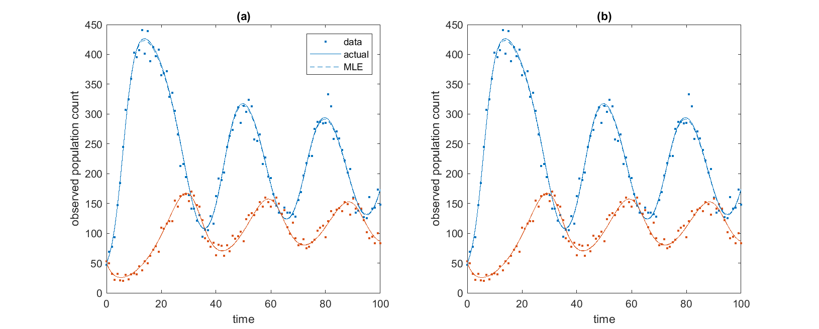
Figure 2: Results for the predator–prey model from: (a) the basic method; (b) the structured method. Each panel shows the solution under the actual parameter values (solid curves); the solution under the maximum likelihood estimate for the parameter values (dashed curves); and the simulated data (dots) for the prey (blue) and predator (red). Where the dashed curve representing the solution at the MLE is not visible, this is because it coincides with the solid curve representing the solution at the true parameter values.

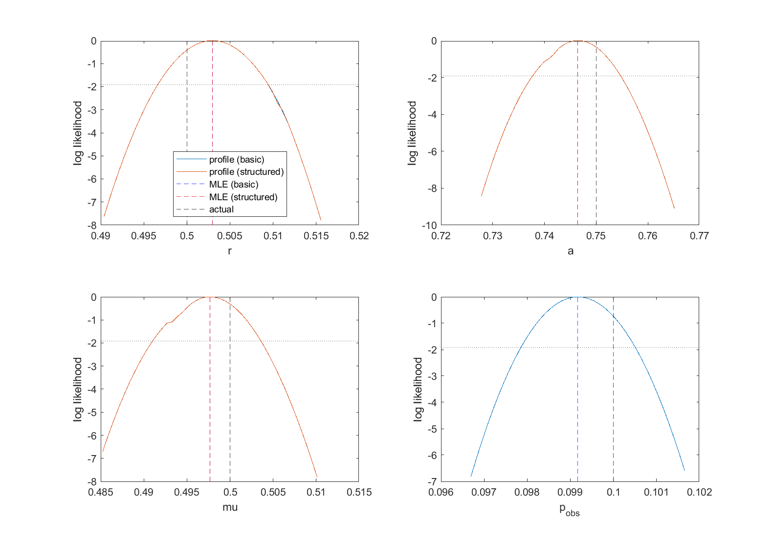
Figure 3: Normalised likelihood profiles for inferred parameters of the predator–prey model: prey intrinsic growth rate ($r$); predation coefficient ($a$); predator death rate ($\mu$); observation probability ($p_{\mathrm{obs}}$). The blue curves are from the basic method; the red curves are from the structured method; dashed vertical lines indicate the actual values (black) and the maximum likelihood estimates for each parameter under the basic method (blue) and structured method (red). Where the blue curve is not visible, this is because it coincides exactly with the red curve. Dotted horizontal line shows the threshold normalised log likelihood for the 95% confidence interval.

Predator-prey model

The model exhibits limit cycle dynamics for the parameter values chosen, completing around three cycles during the time period observed (Figure 2). Both the basic and the structured method were able to successfully recover the correct parameter values from the observed data. The univariate likelihood profiles are almost identical for both methods and are unimodal, implying that the parameters are identifiable (Figure 3). The 95% confidence intervals (range of values above the dotted horizontal line in Figure 3) contained the true parameter value for all target parameters for both methods.

When run on $M=500$ independently generated synthetic datasets, both methods had similar levels of accuracy in the MLE, with a median relative error of $0.5$% (interquartile range [0.3%, 0.7%]) – see Table 1. The coverage properties of both methods were good, with the 95% CI containing the true parameter value in 94–96% of cases for both methods. However, the structured method required only 7492 calls (i.e. evaluations of the forward model) on average, compared to 15054 for the basic method. The reduction in the number of calls for the structured method compared to the basic method was 50.2% (interquartile range [48.5%, 52.1%]). The efficiency improvement was greater in the profile likelihood component of the algorithm than in calculation of the MLE, where the reduction in calls was 18.4% [6.3%, 28.8%]). This is partly because, with the structured method, the inner parameter is effectively a function of the outer parameters (i.e. the solution of the inner optimisation problem in Eq. (5)), so does not need to be profiled separately. However, there was also a reduction in the number of calls per parameter profile.

		Relative error (%)
		Basic	Structured
Predator-prey		0.5 [0.3, 0.7]	0.5 [0.3, 0.7]
SEIR		2.6 [1.3, 4.9]	2.6 [1.2, 4.6]
Adv. diff.		11.0 [6.6, 17.3]	11.0 [6.6, 17.3]
		95% CI coverage
		Basic	Structured
Predator-prey	$r$	94.8%	94.8%
	$a$	94.6%	94.0%
	$\mu$	95.4%	95.2%
	$p_{obs}$	95.4%	-
SEIR	$R_{0}$	89.0%	92.2%
	$w$	87.2%	90.4%
	$p_{obs}$	86.2%	-
	$k$	88.2%	91.8%
Adv. diff.	$D$	89.8%	89.8%
	$v$	90.8%	90.8%
	$R$	90.2%	-
	$\sigma$	88.4%	88.4%
		Function calls (MLE)
		Basic	Structured	Improvement (%)
Predator-prey		208 [194, 228]	171 [153, 194]	18.4 [6.3, 28.8]
SEIR		143 [134, 154]	130 [121, 143]	9.2 [-2.6, 19.5]
Adv. diff.		173 [158, 191]	98 [88, 111]	42.9 [33.9, 50.3]
		Function calls (profiles)
		Basic	Structured	Improvement (%)
Predator-prey		14839 [14084, 15815]	7320 [7017, 7662]	50.7 [49.0, 52.7]
SEIR		13389 [12854, 13750]	7339 [7123, 7545]	44.9 [42.6, 46.7]
Adv. diff.		10247 [9699, 10893]	4675 [4339, 5059]	54.6 [51.5, 56.9]
		Function calls (total)
		Basic	Structured	Improvement (%)
Predator-prey		15054 [14294, 16029]	7492 [7184, 7834]	50.2 [48.5, 52.1]
SEIR		13542 [12998, 13900]	7476 [7251, 7693]	44.5 [42.3, 46.3]
Adv. diff.		10424 [9870, 11064]	4772 [4433, 5158]	54.4 [51.2, 56.7]

Table 1: Relative error in the maximum likelihood estimate, coverage of the 95% CI (i.e. proportion of datasets for which the 95% CI contained true parameter value) for each profiled parameter, and the number of calls to the forward model solver (number to calculate the MLE, number to calculate the likelihood profiles, and total number) under the basic and structured inference methods for each of the three model case studies. Note coverage statistics for the inner parameters ($p_{\mathrm{obs}}$ and $R$) are not applicable for the structured method, as the inner parameter is calculated as a function of the outer parameters. The ‘Improvement’ column shows the reduction in the number of function calls under the structured method relative to the basic method. Results show the median and interquartile range across $M=500$ independently generated datasets for each model.

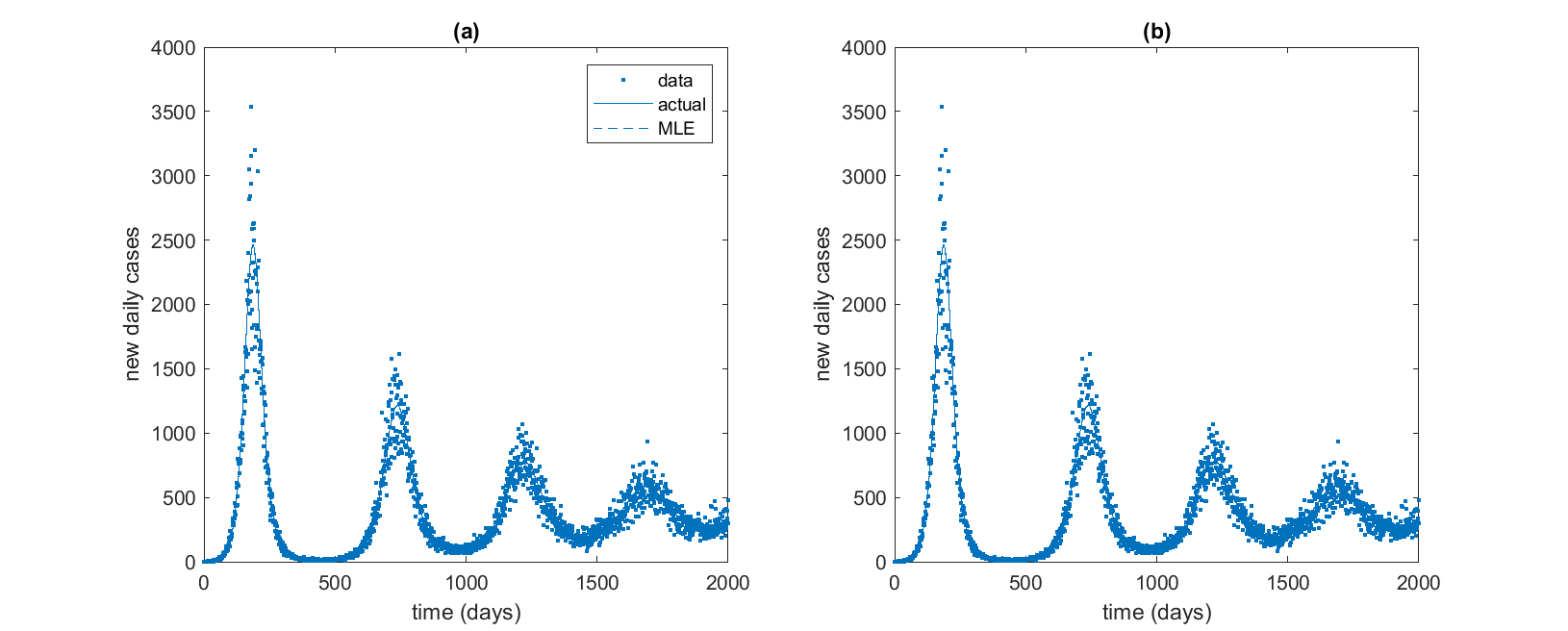
Figure 4: Results for the SEIR model from: (a) the basic method; (b) the structured method. Each panel shows the solution under the actual parameter values (solid curves); the solution under the maximum likelihood estimate for the parameter values (dashed curves); and the simulated data (dots). Where the dashed curve representing the solution at the MLE is not visible, this is because it coincides with the solid curve representing the solution at the true parameter values.

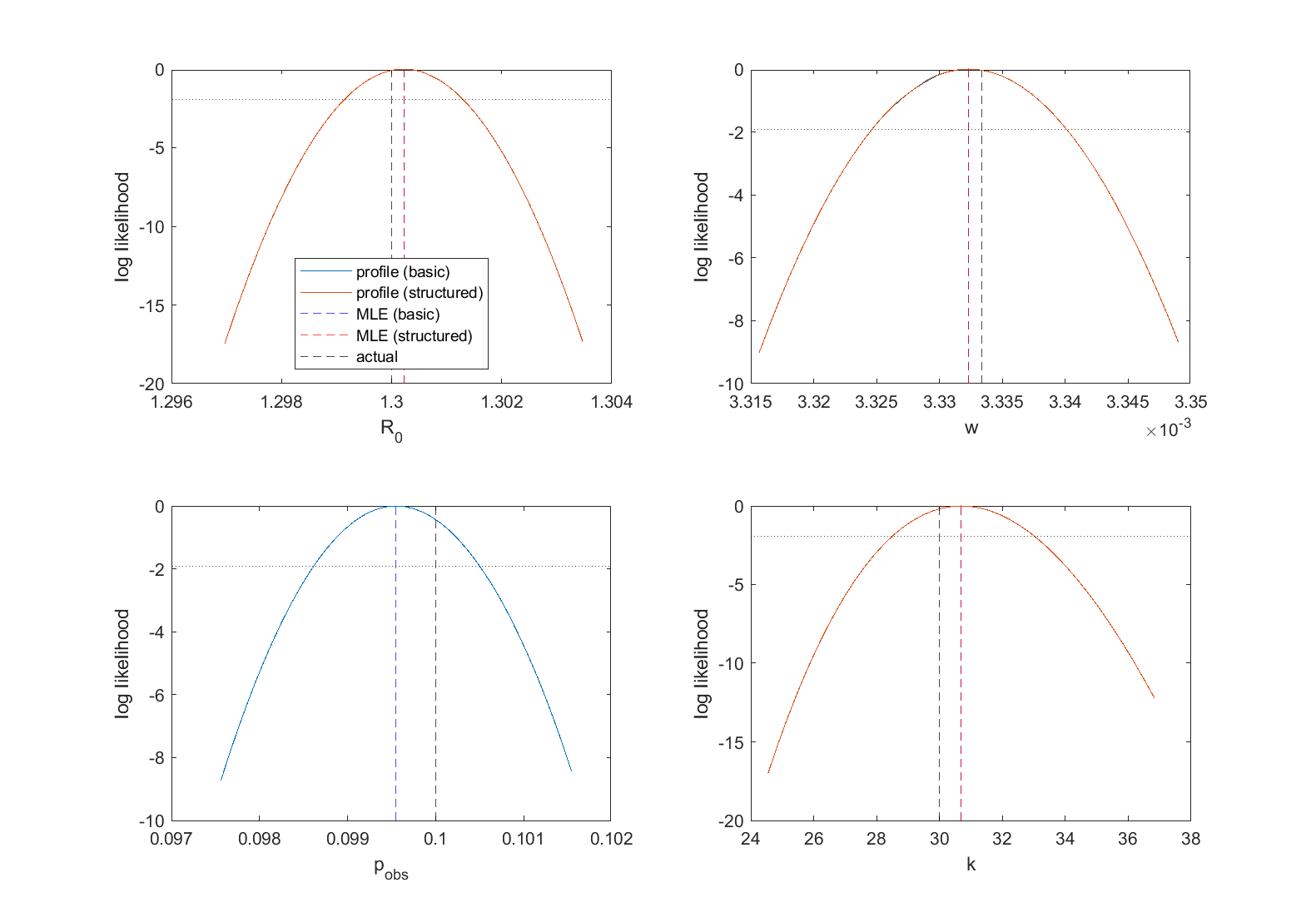
Figure 5: Normalised likelihood profiles for inferred parameters of the SEIR model: basic reproduction number ($R_{0}$); recovered to susceptible rate ($w$); observation probability ($p_{\mathrm{obs}}$); negative binomial dispersion parameter for observed data ($k$). The blue curves are from the basic method; the red curves are from the structured method; dashed vertical lines indicate the actual values (black) and the maximum likelihood estimates for each parameter under the basic method (blue) and structured method (red). Where the blue curve is not visible, this is because it coincides exactly with the red curve. Dotted horizontal line shows the threshold normalised log likelihood for the 95% confidence interval.

SEIR model

The model exhibits a large epidemic wave, followed by a series of successively smaller waves as the model approaches the stable endemic equilibrium (Figure 4). Again, both the basic and the structured method successfully recovered the correct parameter values, and produced almost identical MLEs and univariate likelihood profiles (Figure 5). The profiles were unimodal, meaning that the parameters were identifiable.

When run on $M=500$ independently generated datasets, both methods again had similar accuracy, with a relative error in the MLE of 2.6% [1.3%, 4.9%] for the basic method, compared to 2.6% [1.2%, 4.6%] for the structured method (Table 1). The coverage rates were somewhat below 95%, and were slightly better for the structured method (90–93%) compared to the basic method (86–90%). However, the main advantage of the structured method was its efficiency, with a 44.5% [42.3%, 46.3%] reduction in the total number of calls required compared to the basic method. As for the predator-prey model, most of the efficiency improvement was in the profile likelihood component, although there was also a reduction of 9.2% [-2.6%, 19.5%] in the number of calls required for the MLE.

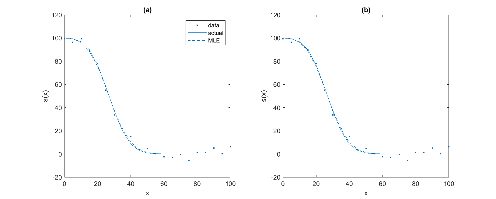
Figure 6: Results for the advection–diffusion model from: (a) the basic method; (b) the structured method. Each panel shows the solution under the actual parameter values (solid curves); the solution under the maximum likelihood estimate for the parameter values (dashed curves); and the simulated data (dots). Where the dashed curve representing the solution at the MLE is not visible, this is because it coincides with the solid curve representing the solution at the true parameter values.

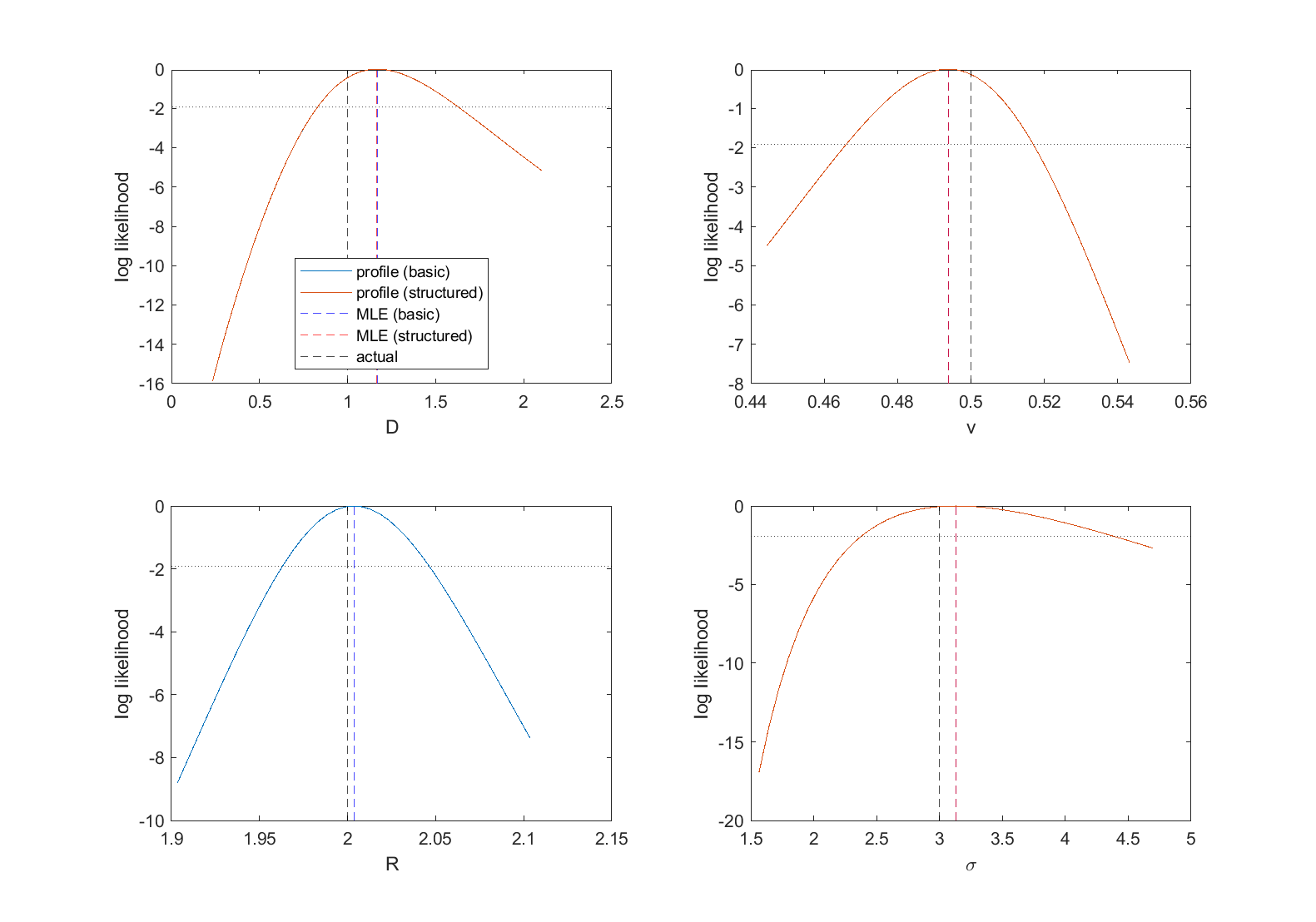
Figure 7: Normalised likelihood profiles for inferred parameters of the advection–diffusion model: diffusion coefficient ($D$); advection velocity ($v$); retardation factor ($R$); standard deviation of noise in observed data ($\sigma$). The blue curves are from the basic method; the red curves are from the structured method; dashed vertical lines indicate the actual values (black) and the maximum likelihood estimates for each parameter under the basic method (blue) and structured method (red). Where the blue curve is invisible, this is because it coincides exactly with the red curve. Dotted horizontal line shows the threshold normalised log likelihood for the 95% confidence interval.

Advection-diffusion model

The model exhibits a sigmoidal decay in concentration with distance from the source at the observation time of $t_{\mathrm{obs}}=100$. (Figure 6). Again, both methods successfully recovered the correct parameter values. Although all univariate likelihood profile were unimodal, the confidence intervals for the diffusion coefficient $D$ and noise magnitude $\sigma$ (range of values above the dotted horizontal line in Figure 7) were relatively wide compared to the other target parameters (Figure 7). This indicates that $D$ and $\sigma$ were relatively weakly identified by the data, and a range of values of these parameters were approximately consistent with the observed data.

When run on $M=500$, independently generated datasets, the relative error was 11.0% [6.6%, 17.3%] for both methods (Table 1). Coverage rates were reasonable (88–91% for the both methods). The structured method required 54.4% [51.2%, 56.7%] fewer calls to the model than the basic method did. Even for the MLE component alone, the structured method provided a substantial improvement in efficiency with 42.9% [33.9%, 50.3%] fewer calls than the basic method.

Sensitivity analysis

The results described above for each model are for $M=500$ independent datasets, each generated using the same set of parameter values. To test the sensitivity of our results to the true parameter values, we repeated the analysis with $M=500$ datasets, each generated from an independently chosen set of parameter values. For each target parameter, we chose the value from an independent normal distribution with the same mean as previously (see Supplementary Table S1) and with coefficient of variation $0.1$.

The results are similar to those described above for fixed parameters. The accuracy and coverage properties are similar for both methods, but the structured method is consistently more efficient than the basic method (see Supplementary Material for details).

Discussion

We have developed an adapted method for likelihood-based parameter inference and uncertainty quantification. The method is based on standard maximum likelihood estimation and profile likelihood, but exploits known structure in the mechanistic model to split a potentially high-dimensional optimisation problem into a nested pair of lower-dimensional problems. Only the outer problem requires the forward model to be solved at each step. Like standard maximum likelihood estimation, our method can be applied with a range of different noise models, provided a likelihood function exists.

We have illustrated the new method on three toy models from different areas of the life sciences: a predator-prey model; a compartment-based epidemic model; and an advection-diffusion model. We have shown that the standard method and the new structured method provided comparable levels of accuracy in parameter estimates and coverage of inferred confidence intervals. However, the structured method was consistently more efficient, requiring substantially fewer calls to the forward model. In more complex models that are computationally expensive to solve, this would provide a major improvement in computation time.

Although we have illustrated our method on three simple models, each with a single inner parameter, we anticipate there will be a broad class of models for which our approach could be applied. These include models where one or more dependent variables are linear in one or more parameters. This was the situation in the first two of our case studies. A similar situation would arise if observed model components were linear in an initial or boundary condition, or in a model with one-way coupling from a nonlinear to a linear component. Our approach is also applicable to models where a parameter effectively rescales one of the independent variables (typically space or time), which was the situation in the third case study. More generally, models which possess some sort of symmetry or invariance may also be candidates for applying our approach. These include travelling wave solutions (such as in models of a spreading population or other reaction–diffusion equations [29, 30]), similarity solutions (such as in models of chemotaxis [31, 32]), or scale invariance (such as in size-spectrum models of marine ecosystem dynamics [33, 34]).

The process of specifying inner parameters and identifying the transformation relationship will in general be model-dependent. In models where such relationships exist, they may be revealed by a non-dimensionalisation procedure, which is a well-established technique in mathematical modelling [35]. A clear example of this would include a broad class of reaction–diffusion models with a logistic source term with carrying capacity $K$, where changing the value of $K$ linearly rescales the solution of the model [36].

Our new method does not avoid the risk of the optimisation routine converging to a local minimum instead of a global minimum. Nonetheless, one way to tackle this is to use a global search algorithm, and using our approach to reduce the dimensionality of the parameter space may help this to succeed.

We have examined case studies in which data come from some specified noise process applied to the solution of an underlying deterministic model. Profile likelihood has also been applied to stochastic models, for example a stochastic model of diffusion in heterogeneous media [1].

In this first presentation of our structured inference approach, we have naturally focused on a range of applications where all parameters are identifiable. However, it will also be possible to apply our methodology to non-identifiable problems. Profile likelihood-based approaches are known to perform reasonably well in the face of non-identifiability whereas other approaches can give misleading results [8]. Another feature of our study is that we have applied our methods to standard cases where we treat the available data as fixed, but we note that we could adapt our method to deal with cases where inference and identifiability analysis is dynamically updated as new data becomes available [37].

In this article, we have focused on parameter estimation and identifiability analysis. Given our univariate profile likelihood functions, it is possible to make profile-wise predictions, propagating uncertainty in parameter estimates through to uncertainty in model predictions [15]. This enables understanding of how variability in different parameters impacts the solution of the mathematical model. Given that our structured profile likelihood functions can be computed with far less computational overhead than the standard approach, it is possible to use our structured approach to speed up the calculation of likelihood-based prediction intervals [15].

Finally, we remark that the work here has been presented in a frequentist, likelihood-based framework for parameter estimation and parameter identifiability analysis. We chose to work in a frequentist framework for the sake of algorithmic simplicity and computational efficiency. However, the results presented here could have been considered within a Bayesian setting by using the relevant likelihood functions within a sampling as opposed to an optimisation approach [38, 39]. Previous direct comparisons for parameter estimation and parameter identifiability suggest that taking a Bayesian approach leads to comparable results to a frequentist likelihood–based approach [8], albeit incurring an increased computational overhead since sampling is, in general, more computationally expensive than optimisation.

Our structured inference approach could, in principle, be used in a Bayesian setting by sampling from the distribution of outer parameters and, for each sample point, optimising the inner parameters using a likelihood or approximate likelihood function. Implementing this is beyond the scope of this paper but would be an interesting aim for future work.

Acknowledgements

MJS is supported by the Australian Research Council (DP230100025). MJP acknowledges travel support from the Australian Research Council (DP200100177) The authors are grateful to the organisers of the 3rd New Zealand Workshop on Uncertainty Quantification and Inverse Problems, held at the University of Canterbury in 2023.

References

- [1] Matthew J Simpson, Alexander P Browning, Christopher Drovandi, Elliot J Carr, Oliver J Maclaren, and Ruth E Baker. Profile likelihood analysis for a stochastic model of diffusion in heterogeneous media. Proceedings of the Royal Society A, 477(2250):20210214, 2021.
- [2] Joseph G Shuttleworth, Chon Lok Lei, Dominic G Whittaker, Monique J Windley, Adam P Hill, Simon P Preston, and Gary R Mirams. Empirical quantification of predictive uncertainty due to model discrepancy by training with an ensemble of experimental designs: an application to ion channel kinetics. Bulletin of Mathematical Biology, 86(1):2, 2024.
- [3] Scott A Sisson, Yanan Fan, and Mark M Tanaka. Sequential monte carlo without likelihoods. Proceedings of the National Academy of Sciences, 104(6):1760–1765, 2007.
- [4] Tina Toni, David Welch, Natalja Strelkowa, Andreas Ipsen, and Michael PH Stumpf. Approximate Bayesian computation scheme for parameter inference and model selection in dynamical systems. Journal of the Royal Society Interface, 6(31):187–202, 2009.
- [5] Mikael Sunnåker, Alberto Giovanni Busetto, Elina Numminen, Jukka Corander, Matthieu Foll, and Christophe Dessimoz. Approximate Bayesian computation. PLoS Computational Biology, 9(1):e1002803, 2013.
- [6] Keegan E Hines, Thomas R Middendorf, and Richard W Aldrich. Determination of parameter identifiability in nonlinear biophysical models: A bayesian approach. Journal of General Physiology, 143:401–416, 2014.
- [7] Ivo Siekmann, James Sneyd, and EC Crampin. Mcmc can detect nonidentifiable models. Biophysical Journal, 103:2275–2286, 2012.
- [8] Matthew J Simpson, Ruth E Baker, Sean T Vittadello, and Oliver J Maclaren. Practical parameter identifiability for spatio-temporal models of cell invasion. Journal of the Royal Society Interface, 17(164):20200055, 2020.
- [9] Andreas Raue, Clemens Kreutz, Fabian Joachim Theis, and Jens Timmer. Joining forces of bayesian and frequentist methodology: a study for inference in the presence of non-identifiability. Philosophical Transactions of the Royal Society A: Mathematical, Physical and Engineering Sciences, 371:20110544, 2013.
- [10] DG Bates DM abd Watts. Nonlinear regression analysis and its applications. Wiley, 1988.
- [11] Andreas Raue, Clemens Kreutz, T Maidwald, J Bachmann, M Schilling, U Klingmüller, and J Timmer. Structural and practical identifiability analysis of partially observed dynamical models by exploiting the profile likelihood. Bioinformatics, 25:1923–1929, 2009.
- [12] C Kreutz, A Raue, D Kaschek, and J Timmer. Profile likelihood in systems biology. The FEBS Journal, 280:2564–2571, 2013.
- [13] C Kreutz, A Raue, and J Timmer. Likelihood based observability analysis and confidence intervals for predictions of dynamics models. BMC Systems Biology, 6:120, 2013.
- [14] M V Ciocanel, L Ding, K Mastromatteo, S Reicheld, S Cabral, K Mowry, and B Standtede. Parameter identifiability in pde models of fluorescence recovery after photobleaching. Bulletin of Mathematical Biology, 86:36, 2024.
- [15] Matthew J Simpson and Oliver J Maclaren. Profile-wise analysis: A profile likelihood-based workflow for identifiability analysis, estimation, and prediction with mechanistic mathematical models. PLoS Computational Biology, 19(9):e1011515, 2023.
- [16] Audrey Lustig, Giorgia Vattiato, Oliver Maclaren, Leighton M Watson, Samik Datta, and Michael J Plank. Modelling the impact of the Omicron BA.5 subvariant in New Zealand. Journal of the Royal Society Interface, 20(199):20220698, 2023.
- [17] Yudi Pawitan. In all likelihood: Statistical modelling and inference using likelihood. Oxford University Press, 2001.
- [18] Patrick Royston. Profile likelihood for estimation and confidence intervals. The Stata Journal, 7:376–387, 2007.
- [19] Michael L Rosenzweig and Robert H MacArthur. Graphical representation and stability conditions of predator-prey interactions. American Naturalist, 97(895):209–223, 1963.
- [20] Alfred James Lotka. Elements of Physical Biology. Williams & Wilkins, 1925.
- [21] Vito Volterra. Variazioni e fluttuazioni del numero d’individui in specie animali conviventi. Memoria della Reale Accademia Nazionale dei Lincei, 2:31–113, 1926.
- [22] Odo Diekmann and Johan Andre Peter Heesterbeek. Mathematical epidemiology of infectious diseases: model building, analysis and interpretation. Wiley, 5th edition, 2000.
- [23] Timothy W Russell, Nick Golding, Joel Hellewell, Sam Abbott, Lawrence Wright, Carl AB Pearson, Kevin van Zandvoort, Christopher I Jarvis, Hamish Gibbs, Yang Liu, Rosalind M Eggo, W J Edmunds, Adam J Kucharski, and CMMID COVID-19 working group. Reconstructing the early global dynamics of under-ascertained COVID-19 cases and infections. BMC Medicine, 18(1):332, 2020.
- [24] Seth Flaxman, Swapnil Mishra, Axel Gandy, H Juliette T Unwin, Thomas A Mellan, Helen Coupland, Charles Whittaker, Harrison Zhu, Tresnia Berah, Jeffrey W Eaton, et al. Estimating the effects of non-pharmaceutical interventions on COVID-19 in Europe. Nature, 584(7820):257–261, 2020.
- [25] Jorg Herzer and Wolfgang Kinzelbach. Coupling of transport and chemical processes in numerical transport models. Geoderma, 44:473–480, 1976.
- [26] A Ogata and R B Banks. A solution of the differential equation of longitudinal dispersion in porous media. US Geological Survey, Professional Paper, 411-A, 1961.
- [27] M T Van Genuchten and P J Wierenga. Mass transfer studies in sorbing porous media i. analytical solutions. Soil Science Society of America Journal, 40:115–127, 1989.
- [28] R J Murphy, O J Maclaren, and M J Simpson. Implementing measurement error models with mechanistic mathematical models in a likelihood-based framework for estimation and prediction in the life sciences. Journal of the Royal Society Interface, 21:20230402, 2024.
- [29] Ruth E Baker and P K Maini. Travelling gradients in interacting morphogen systems. Mathematical Biosciences, 209(1):30–50, 2007.
- [30] Ruth E Baker and Matthew J Simpson. Models of collective cell motion for cell populations with different aspect ratio: diffusion, proliferation and travelling waves. Physica A: Statistical Mechanics and its Applications, 391(14):3729–3750, 2012.
- [31] M Rascle and C Ziti. Finite time blow-up in some models of chemotaxis. Journal of Mathematical Biology, 33:388–414, 1995.
- [32] H M Byrne, G Cave, and D L S McElwain. The effect of chemotaxis and chemokinesis on leukocyte locomotion: A new interpretation of experimental results. Mathematical Medicine and Biology: A Journal of the IMA, 15(3):235–256, 1998.
- [33] José A Capitán and Gustav W Delius. Scale-invariant model of marine population dynamics. Physical Review E, 81(6):061901, 2010.
- [34] Michael John Plank and Richard Law. Ecological drivers of stability and instability in marine ecosystems. Theoretical Ecology, 5:465–480, 2012.
- [35] James D Murray. Mathematical Biology: I: An Introduction. Springer, 2003.
- [36] P Haridas, C J Penington, J A McGovern, D L S McElwain, and M J Simpson. Quantifying rates of cell migration and cell proliferation in co-culture barrier assays reveals how skin and melanoma cells interact during melanoma spreading and invasion. Journal of Theoretical Biology, 423:13–25, 2017.
- [37] T Cassudy. A continuation technique for maximum likelihood estimators in biological models. Bulletin of Mathematical Biology, 85:90, 2023.
- [38] A Gelman, A Vehtari, D Simpson, C C Margossian, B Carpenter, Y Yao, L Kennedy, J Gabry, P-C Bürkner, and M Modrák. Bayesian workflow. arXiv preprint, 2011.01808, 2020.
- [39] Larry Wasserman. All of Statistics: A Concise Course in Statistical Inference. Springer, 2004.