Geometry and Stability of Supervised Learning Problems

Abstract

We introduce a notion of distance between supervised learning problems, which we call the Risk distance. This optimal-transport-inspired distance facilitates stability results; one can quantify how seriously issues like sampling bias, noise, limited data, and approximations might change a given problem by bounding how much these modifications can move the problem under the Risk distance. With the distance established, we explore the geometry of the resulting space of supervised learning problems, providing explicit geodesics and proving that the set of classification problems is dense in a larger class of problems. We also provide two variants of the Risk distance: one that incorporates specified weights on a problem’s predictors, and one that is more sensitive to the contours of a problem’s risk landscape.

Keywords: supervised learning, stability, metric geometry, optimal transport, risk landscape

1 Introduction

In machine learning, even before beginning work on a problem, we are often forced to accept discrepancies between the problem we want to solve and the problem we actually get to work with. We may put up with noise or bias in the data collection process which distorts our view of the true distribution of observations. We may replace a loss function with a surrogate loss whose computational cost or optimization properties are preferable. We may have access to only a small sample of observations. Such compromises are a necessary reality.

This brings us to our primary motivating questions.

• Question 1: How much can such a compromise change our problem and its descriptive features?

• Question 2: How much effect can multiple compromises have in conjunction? Can we guarantee that a sequence of small changes will not have drastic effects on the problem to be solved?

1.1 Overview of our approach.

In this paper, we provide a comprehensive framework with which to answer such questions. While many frameworks exist to answer Question 1, these methods are concerned with quantifying changes to one or two aspects of a problem at a time, limiting their ability to answer Question 2. In real world problems, multiple simultaneous corruptions and substitutions are unavoidable. Our framework is broad enough to handle simultaneous changes to many aspects of a problem. To begin, we give a precise definition of “supervised learning problem” and define a notion of distance, dubbed the Risk distance and denoted $d_{\mathrm{R}}$, by which to compare pairs of problems. This gives rise to the (pseudo)metric space of supervised learning problems. The Risk distance lets us make geometric sense of Questions 1 and 2; we can measure how much a compromise affects a problem by seeing how far the problem moves under the Risk distance.

To actually define the Risk distance $d_{\mathrm{R}}$, we draw on the wisdom of metric geometry. In 1975, Edwards constructed a metric on the set of isomorphism classes of compact metric spaces which came to be known as the Gromov-Hausdorff distance (Edwards, 1975; Gromov, 1981). Similarly, the Gromov-Wasserstein distance, introduced by Mémoli (2007, 2011), provides an optimal-transport-based metric on the collection of isomorphism classes of metric spaces equipped with probability measures. The Gromov-Hausdorff and Gromov-Wasserstein distances have become integral to the theory of metric geometry by facilitating a geometric understanding of spaces in which the points themselves are spaces.

Inspired by this tradition, we craft the Risk distance in the image of the Gromov-Wasserstein distance. This sets up the following analogy between supervised learning and metric geometry.

Supervised Learning Metric Geometry

Problem $$\longleftrightarrow\text{Metric measure space}$$

Loss function $$\longleftrightarrow\text{Metric}$$

Risk distance $$\longleftrightarrow\text{Gromov-Wasserstein distance}$$

1.2 Previous approaches.

Question 1 has previously been explored for various specific kinds of changes to a problem. In our work, a supervised learning problem (or just problem, for short), is modeled as a 5-tuple $P=(X,Y,\eta,\ell,H)$ where $X$ and $Y$ are the input space and response space respectively, $\eta$ is the joint law: a probability measure on $X\times Y$, $\ell$ is the loss function and $H$ is the predictor set: a collection of functions $h:X\to Y$.

• Joint law $\eta$. A common assumption in machine learning is that the data is drawn according to an unknown underlying probability measure. Concepts such as noise and bias in data collection or data shift phenomena such as covariate shift, label shift, or concept drift (Huyen, 2022, Ch 8), can be described as changes to this underlying measure. The effects of various kinds of noise (Zhu and Wu, 2004; Natarajan et al., 2013; Menon et al., 2015, 2018; Rooyen and Williamson, 2018; Iacovissi et al., 2023) and data shifts (Shimodaira, 2000) on supervised learning problems is a longstanding area of research. A geometric framework for understanding changes in probability measures exists as well; information geometry seeks to understand spaces of probability measures from the viewpoint of Riemannian geometry (Amari, 2016; Ay et al., 2017).

• Loss function $\ell$. A theoretically attractive loss may have poor optimization properties, prompting one to replace it with a so-called surrogate loss. Alternatively, an attractive loss could be expensive to exactly compute, making it a candidate for approximation, like replacing a Wasserstein-based loss with a Sinkhorn-based loss in probability estimation (Cuturi, 2013). Replacing the loss represents a tradeoff between theoretical properties and computational efficiency, and the quantitative details of this tradeoff have been explored in many contexts (Lin, 2004; Zhang, 2004; Bartlett et al., 2006; Steinwart, 2007; Awasthi et al., 2022; Mao et al., 2023).

• Predictor set $H$. Universal approximation theorems, popular in deep learning, establish that certain classes of models can approximate large classes of predictors arbitrarily well (Pinkus, 1999). These can be seen as theorems which compare large, intractable predictor sets to those that can be produced by a given model, aiming to show that there is effectively no difference between selecting a predictor from either set. Approximation theory more broadly is similarly concerned with the approximation power of function classes or transforms (Trefethen, 2019).

• Input and response spaces $X$ and $Y$. Modifications of the input and response spaces are implicit in many of the modifications listed above. Additionally, the process of feature engineering (Huyen, 2022, Ch 5), for which there is little established theory, can be seen as a modification of the input space. Examples of output space modification include the common relaxation of classification to class probability estimation or, less common, the discretization of the response space into a finite set of labels (Langford and Zadrozny, 2005) which served as a motivation for the exact results by Reid and Williamson (2011).

• Combinations. Our notion of a learning problem comprises five separate components. There are some existing results that explore how changes to some components affect the others. Some of this work goes under the name of “Machine Learning Reductions” (Langford, 2009). There are results on how changes to the distribution of examples $\eta$ (due to “noise”) has the effect of changing the loss function $\ell$ (with label noise) (van Rooyen and Williamson, 2018) or the model class $H$ (with attribute noise) (Bishop, 1995; Dhifallah and Lu, 2021; Rothfuss et al., 2019; Smilkov et al., 2017; Williamson and Cranko, 2022).

Figure 1: A simple depiction of how a sequence of changes can push a particular problem through the space of problems. An idealized problem $P$ is modified by a sequence of four changes, each change moving the problem some distance in the space of problems. Once the sequence of corruptions has been applied, we call the resulting problem $P^{\prime}$. The original and corrupted problems are connected by a dashed line representing the risk distance between them.

There is precedent for geometric frameworks regarding statistical learning. We have mentioned the rise of information geometry as a way to understand statistical manifolds. Also, much as we aim to do with supervised learning problems, Le Cam developed a notion of distance (Le Cam, 1964; Mariucci, 2016) between the “statistical experiments” of Blackwell (Blackwell, 1951). A modified discrepancy incorporating a loss function was introduced by Torgersen (1991, Complement 37). We will discuss the relationship between supervised learning problems and statistical experiments in Section 3.2.

While much research has sought to quantify and control the effects of various specific corruptions on supervised learning problems, no framework so far has been comprehensive enough to consider changes to all aspects of a problem. That is, while many have given answers to Question 1, to the best of our knowledge no attempt has been made at a unified answer to Question 2.

1.3 Our contributions.

We provide a geometric framework with which to answer both Questions 1 and 2 in the form of the Risk distance.

Our primary tool for answering Question 1 with the Risk distance is the central topic of Section 4: stability results. A stability result is an upper bound on how much a certain change to a problem can move that problem under the Risk distance. That is, if we apply a certain change to a problem $P$ to obtain a new problem $P^{\prime}$, such as a change to the loss function, the data collection process, or the set of potential predictors, a stability result is an upper bound on $d_{\mathrm{R}}(P,P^{\prime})$. Such a result acts as a quantitative guarantee that a small change to some aspect of the problem will not drastically change the problem as a whole.

Comparing problems via a metric also presents advantages over more general kinds of dissimilarity scores: the triangle inequality lets one string together upper bounds on distances. To wit, let $x_{0}$ be a point in a metric space $(X,d_{X})$. Suppose we create a sequence of points $x_{0},x_{1},\dots,x_{k}$ by pushing each point $x_{i-1}$ a distance of at most $\varepsilon$ to get the next point $x_{i}$ in the sequence. Then the triangle inequality assures us that

$$d_{X}(x_{0},x_{k})\leq\sum_{i=1}^{k}d_{X}(x_{i-1},x_{i})\leq k\varepsilon.$$

In other words, in a metric space, a short sequence of small pushes cannot add up to a drastic change. In the context of the Risk distance, this feature lets us handle multiple simultaneous changes to a problem by applying the triangle inequality and stringing together stability results. This gives an answer to Question 2. See Figure 1 for an illustration. By design, the Risk distance will be a pseudometric (that is, a metric for which distinct points can be distance zero apart), but the above virtues of metric spaces apply to pseudometric spaces as well.

Along with stability of the Risk distance under various problem modifications, Section 4 will also demonstrate stability of certain descriptors of learning problems with respect to the Risk distance. In particular, we prove in Section 4.1 that a descriptor of a problem called its constrained Bayes risk is stable under the Risk distance. In other words, if the Risk distance between two problems $P$ and $P^{\prime}$ is less than $\varepsilon$, then the optimal expected loss across all predictors for $P$ is within $\varepsilon$ of that of $P^{\prime}$; see Figure 2 for an illustration. We obtain this stability result by first proving stability under the Risk distance of a stronger descriptor, called the loss profile set of a problem, which describes the possible distributions of losses incurred by a random observation. We also demonstrate stability under the Risk distance of a descriptor from statistical learning theory known as the Rademacher complexity for arbitrarily large sample sizes.

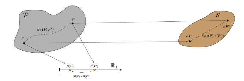
Figure 2: The space $\mathcal{P}$ of all supervised learning problems and a descriptor. A descriptor is modeled as a map $s:\mathcal{P}\to\mathcal{S}$ whose codomain is some metric space $(\mathcal{S},d_{\mathcal{S}})$. A descriptor $s$ is regarded as stable if there is some constant $C>0$ such that $C\,d_{\mathrm{R}}(P,P)\geq d_{\mathcal{S}}(s(P),s(P^{\prime}))$ for all $P,P^{\prime}\in\mathcal{P}$. The figure also depicts the case when $\mathcal{S}$ is the set $\mathbb{R}_{+}$ of non-negative reals and $s(P)$ is the constrained Bayes risk ${\mathcal{B}}(P)$ of $P$. In that case, one of our stability results (Theorem 4.3) establishes that $d_{\mathrm{R}}(P,P^{\prime})\geq\big{|}{\mathcal{B}}(P)-{\mathcal{B}}(P^{\prime})\big{|}$ for all $P,P^{\prime}\in\mathcal{P}.$

In addition to facilitating stability results, the Risk distance gives us a notion of convergence for supervised learning problems. Just as it is fruitful to discuss the convergence of sequences of functions, random variables, or probability distributions, so too can it be useful to discuss the convergence of a sequence of problems. In Section 5.4, we will demonstrate an analog of the Glivenko–Cantelli theorem by proving that the “empirical problem,” a problem constructed using a finite random sample of observations instead of the true distribution from which it is sampled, converges to the “true problem” under the Risk distance with probability 1.

Lastly, the Risk distance lets us consider the geometry of the space of problems and consequences thereof. In Sections 5.1 and 5.2, we connect the geometric concept of a geodesic between two problems with the probabilistic notion of couplings of distributions associated with those problems. This connection lets us write down some explicit geodesics in the space of problems. In Section 5.3, we show that classification problems, meaning those problems with a finite output space, are dense in a larger space of problems under the Risk distance. This density result proves useful when establishing the convergence of empirical problems.

In the final two sections, we also study two variants of the Risk distance. In Section 6, we define a parameterized family of distances, each called the $L^{p}$-Risk distance for $p\in[1,\infty]$. The $L^{p}$-Risk distance incorporates weights in the form of a specified probability measure on the set of possible predictors. The use of this additional data results in improved stability when compared to the Risk distance. In Section 7, we also define a stronger version of the Risk distance, called the Connected Risk distance, which is designed to be more sensitive to changes in the risk landscape of a problem. In particular, we show that a topological summary of the problem called its Reeb graph is stable under the Connected Risk distance.

We regard the Risk distance as tool to produce theoretical guarantees. To prove that problems are stable under a certain kind of change with respect to the Risk distance, or that certain descriptors are stable under the Risk distance, we need only bound the Risk distance above or below. The utility of the Risk distance lies not in explicit algorithms and associated computations, but in the theoretical landscape that it facilitates.

1.4 Other previous work.

Kleinberg’s seminal paper (Kleinberg, 2002) initiated a thread of research into the formal study of clustering problems (Carlsson and Mémoli, 2010, 2013; Ackerman, 2012; Cohen-Addad et al., 2018). In a spirit similar to this thread, the present paper aims to formally examine supervised learning problems.

The Risk distance introduced in this paper participates in a growing thread of research into optimal-transport-based distances, a thread which begins with the metrics discussed in Section 2.3 and runs through more recent variants including optimal transport distances for graph-based data (Chowdhury and Mémoli, 2019; Chen et al., 2022), matrices (Peyré et al., 2016), partitioned data sets (Chowdhury et al., 2021), labeled data sets (Alvarez-Melis and Fusi, 2020), optimal transport of both data and features jointly (Vayer et al., 2020b), or of data with quite general structures (Vayer et al., 2020a; Patterson, 2020), as well as approximations (Scetbon et al., 2021; Sejourne et al., 2021; Vincent-Cuaz et al., 2021) and regularizations (Peyré et al., 2016) thereof.

1.5 Statement of contribution

The genesis of this project dates back to 2010-2011 when F.M. visited R.W. at NICTA (Canberra, Australia). The formulation of the results, finding the proofs, and the vast majority of the writing of the paper was done by F.M. and B.V. R.W. contributed the initial formulation of the question to be addressed, provided some context from the ML literature, and reviewed and slightly revised the final document.

Contents

1. 1 Introduction
   1. 1.1 Overview of our approach.
   2. 1.2 Previous approaches.
   3. 1.3 Our contributions.
   4. 1.4 Other previous work.
   5. 1.5 Statement of contribution
2. 2 Background
   1. 2.1 Preliminary Notation
   2. 2.2 Pushforward Measures, Correspondences, and Couplings
   3. 2.3 Metric Geometry and Optimal Transport
      1. 2.3.1 Hausdorff Distance
      2. 2.3.2 Gromov-Hausdorff Distance
      3. 2.3.3 Wasserstein Distance
      4. 2.3.4 Gromov-Wasserstein Distance
   4. 2.4 Total Variation Distance
   5. 2.5 Markov Kernels
   6. 2.6 Empirical Measures and Glivenko–Cantelli Classes
3. 3 The Risk Distance
   1. 3.1 Problems
   2. 3.2 Comparison with Blackwell’s Statistical Experiments
   3. 3.3 Motivating Properties
   4. 3.4 The Risk Distance
   5. 3.5 Connections to the Gromov-Wasserstein Distance
4. 4 Stability
   1. 4.1 Stability of the Constrained Bayes Risk and Loss Profile
   2. 4.2 Stability of Rademacher Complexity
   3. 4.3 Stability under Sampling Bias
   4. 4.4 Stability under Sampling Noise
   5. 4.5 Stability under Modification of Predictor Set
5. 5 Geometry of the Space of Problems
   1. 5.1 Geodesics
   2. 5.2 Existence of Optimal Couplings and Correspondences
   3. 5.3 Density of Classification Problems
   4. 5.4 Convergence of Empirical Problems
6. 6 The $L^{p}$-Risk Distance: Weighting Problems
   1. 6.1 Weighting Predictor Sets and the $L^{p}$-Risk Distance
   2. 6.2 Connection to the Gromov-Wasserstein Distance
   3. 6.3 Stability of Loss Profile Distribution
   4. 6.4 Improved Density
   5. 6.5 Improved Stability
7. 7 The Connected Risk Distance: Risk Landscapes
   1. 7.1 Insensitivities of the Risk distance
   2. 7.2 The Connected Risk distance
   3. 7.3 Risk Landscapes and Reeb Graphs
8. 8 Discussion
9. A Relegated Proofs
   1. A.1 Proofs and Details from Section 3
      1. A.1.1 Connecting the Risk Distance with the Gromov-Wasserstein Distance
   2. A.2 Proofs from Section 4
   3. A.3 Proofs from Section 5
   4. A.4 Proofs from Section 6
   5. A.5 Proofs from Section 7
10. B Weak Isomorphism with Classification Problems

2 Background

We begin with some necessary concepts and notation from measure theory, metric geometry, and optimal transport. We refer the reader to the standard reference of Villani (2003) for more on measure-theoretic and optimal transport concepts, and that of Burago, Burago, and Ivanov (2001) for metric geometry concepts.

2.1 Preliminary Notation

We use $\pi_{i}$ to represent a projection map $X_{1}\times X_{2}\times\dots\times X_{n}\to X_{i}$ onto the $i$th component of a product. More generally, $\pi_{i_{1},\dots,i_{k}}X_{1}\times\dots\times X_{n}\to X_{i_{1}}\times\dots\times X_{i_{k}}$ represents the projection onto coordinates $i_{1},\dots,i_{k}$.

When integrating a measurable function $f$ against a measure $\mu$, we will favor the notation

$$\int_{X\times Y}f(x,y)\,\mu(dx\times dy)$$

if $f$ is a function of two variables, and similarly for more variables. We often suppress the domain of integration under the integral symbol since it is implicit in the measure $\mu$. Rarely, when many variables are necessary and horizontal space is at a premium, we may instead use the notation

$$\int f(x,y)\,d\mu(x,y).$$

Given a measurable space $(Z,\Sigma_{Z})$, we let $\operatorname{Prob}(Z)$ denote the space of probability measures on $(Z,\Sigma_{Z})$. For any $z\in Z$, we let $\delta_{z}\in\operatorname{Prob}(Z)$ denote the Dirac probability measure at $z$ defined, for $A\in\Sigma_{Z}$, as $\delta_{z}(A)=1$ whenever $z\in A$ and as $0$ otherwise. Given a probability measure $\alpha\in\operatorname{Prob}(\mathbb{R})$, we let $\mathrm{mean}(\alpha):=\int_{\mathbb{R}}t\,\alpha(dt)$ denote its mean whenever it exists.

2.2 Pushforward Measures, Correspondences, and Couplings

We recall some basic ideas from measure theory and establish notation. Given a measure space $(X,\Sigma_{X},\mu)$, a measurable space $(Y,\Sigma_{Y})$, and a measurable map $f:X\to Y$, the pushforward of $\mu$ through $f$ is the measure on $(Y,\Sigma_{Y})$ defined by

$$f_{\sharp}\mu(A):=\mu(f^{-1}(A))$$

for all $A\in\Sigma_{Y}$. If $\mu$ is a probability measure, $f_{\sharp}\mu$ will be a probability measure as well. Hence $f_{\sharp}$ is a function $\operatorname{Prob}(X)\to\operatorname{Prob}(Y)$. A pushforward has a probabilistic interpretation: if $\mathsf{X}$ is a random variable in a measurable space $X$ with law $\mu$, and $f:X\to Y$ is measurable, then the random variable $f(\mathsf{X})$ has law $f_{\sharp}\mu$.

Given two sets $X$ and $Y$, a subset $R\subseteq X\times Y$ is called a correspondence if

• for all $x\in X$ there is some $y\in Y$ with $(x,y)\in R$, and

• for all $y\in Y$ there is some $x\in X$ with $(x,y)\in R$.

We use ${\mathcal{C}}(X,Y)$ to denote the set of all correspondences between $X$ and $Y$.

A coupling between two probability measure spaces $(X,\Sigma_{X},\mu_{X})$ and $(Y,\Sigma_{Y},\mu_{Y})$ is a probability measure on $X\times Y$ with marginals $\mu_{X}$ and $\mu_{Y}$. That is, a probability measure $\gamma$ on $X\times Y$ is a coupling if the pushforward measures satisfy $(\pi_{1})_{\sharp}\gamma=\mu_{X}$, $(\pi_{2})_{\sharp}\gamma=\mu_{Y}$. We use $\Pi(\mu_{X},\mu_{Y})$ to denote the set of all such measures. Couplings can be seen as a probabilistic counterpart to correspondences.

The following are standard methods for constructing correspondences between two sets $X$ and $Y$.

• The entire product $X\times Y$ is always a correspondence. In particular, this shows that ${\mathcal{C}}(X,Y)$ cannot be empty.

• If $X=Y$, one can construct the diagonal correspondence $\left\{(x,x)\middle|x\in X\right\}$.

• If $Y=\{\bullet\}$ is the one point set, then there is a unique correspondence $X\times\{\bullet\}$.

• The graph of any surjection $f:X\to Y$ is a correspondence between $X$ and $Y$.

Analogous constructions exist for couplings as well. Let $(X,\mu_{X})$ and $(Y,\mu_{Y})$ be probability spaces.

• The product measure $\mu_{X}\otimes\mu_{Y}$ is always a coupling, sometimes called the independent coupling. This shows that $\Pi(\mu_{X},\mu_{Y})$ cannot be empty.

• Suppose $(X,\mu_{X})=(Y,\mu_{Y})$. If $\Delta_{X}:X\to X\times X$ denotes the diagonal map $\Delta_{X}(x)=(x,x)$, then the diagonal coupling is the pushforward measure $(\Delta_{X})_{\sharp}\mu_{X}$.

• If $Y=\{\bullet\}$ is the one point set, then forcibly $\mu_{Y}=\delta_{\bullet}$ and there is a unique coupling $\mu_{X}\otimes\delta_{\bullet}$ in this case.

• Suppose $f:X\to Y$ is a measure-preserving map, meaning $f_{\sharp}\mu_{X}=\mu_{Y}$. Let $i_{f}:X\to X\times Y$ be the map sending $X$ to the graph of $f$, meaning $i_{f}(x):=(x,f(x))$. Then the pushforward $(i_{f})_{\sharp}\mu_{X}$ is a coupling between $\mu_{X}$ and $\mu_{Y}$.

When we discuss Markov kernels in Section 2.5, we will mention one more method for generating couplings by combining a probability measure $\alpha\in\operatorname{Prob}(X)$ and a Markov Kernel $\beta:X\to\operatorname{Prob}(Y)$ using reverse disintegration.

We will make use of the following standard coupling result, which can be found in any standard optimal transport text, such as that of Villani (2003, Lemma 7.6). Note that a topological space is called Polish if it is separable and metrizable by a complete metric. Most familiar spaces are Polish, including $\mathbb{R}^{n}$ and open subsets thereof, manifolds with or without boundary, and finite discrete spaces. A Borel measurable space arising from a Polish topological space is called Polish as well.

Proposition 2.1 (The Gluing Lemma).

Let $\mu_{1}$, $\mu_{2}$ and $\mu_{3}$ be probability measures on Polish spaces $X_{1}$, $X_{2}$, and $X_{3}$ respectively. Let $\gamma_{1,2}\in\Pi(\mu_{1},\mu_{2})$ and $\gamma_{2,3}\in\Pi(\mu_{2},\mu_{3})$. Then there exists a probability measure $\gamma_{1,2,3}$ on $X_{1}\times X_{2}\times X_{3}$ with marginals $\gamma_{1,2}$ on $X_{1}\times X_{2}$ and $\gamma_{2,3}$ on $X_{2}\times X_{3}$.

We call such a $\gamma_{1,2,3}$ a gluing of $\gamma_{1,2}$ and $\gamma_{2,3}$. An analog of the gluing lemma for correspondences (see Burago et al., 2001, Exercise 7.3.26) instead of couplings is included below in order to highlight the parallels between couplings and correspondences.

Proposition 2.2 (The Gluing Lemma for Correspondences).

Let $A_{1}$, $A_{2}$ and $A_{3}$ be sets, and let $R_{1,2}\in{\mathcal{C}}(A_{1},A_{2})$ and $R_{2,3}\in{\mathcal{C}}(A_{2},A_{3})$. Then there exists a subset $R_{1,2,3}\subseteq A_{1}\times A_{2}\times A_{3}$ which projects to $R_{1,2}$ on $A_{1}\times A_{2}$ and $R_{2,3}$ on $A_{2}\times A_{3}$.

We call such an $R_{1,2,3}$ a gluing of $R_{1,2}$ and $R_{2,3}$.

Proof.

Selecting $R_{1,2,3}=\left\{(x,y,z)\in A_{1}{\times}A_{2}{\times}A_{3}\middle|(x,y)\in R_{1,2},(y,z)\in R_{2,3}\right\}$ provides one such subset. ∎

In this paper, all of our measurable spaces will arise from Polish topological spaces by equipping the space with the Borel $\sigma$-algebra. For this reason, we will suppress the $\sigma$-algebra in our notation for measure spaces. That is, if $X$ is a Polish topological space equipped with a Borel measure $\mu$, instead of the triple $(X,\Sigma_{X},\mu)$, we will write $(X,\mu)$ with the understanding that the underlying $\sigma$-algebra is the Borel $\sigma$-algebra. In this context, we define the support of the measure $\mu$ as

$$\mathrm{supp}[\mu]:=\{x\in X\,|\,\mu(U)>0\,\forall\,U\,\mbox{open s.t.}\,x\in U\}.$$

2.3 Metric Geometry and Optimal Transport

Here we present four metrics from the field of metric geometry. The following diagram (inspired by Mémoli, 2011, Fig. 2) illustrates the relationships between the four metrics.

We do not explicitly use the Gromov-Hausdorff or Gromov-Wasserstein distances in this paper. However, these distances provide context by illustrating common threads that run through all four metrics and is shared by the Risk distance. In all four of the metrics, objects are compared by optimally “aligning” the two objects, whether via correspondences or couplings, and numerically scoring the distortion incurred by an optimal alignment. The Risk distance (Definition 3.13) follows this same template. To emphasize the continuation of this thread, we will take a moment to compare the Risk distance to the Gromov-Wasserstein distance in Section 3.5.

Note that we will often suppress the underlying metric in our notation, writing a metric space $(X,d_{X})$ as simply $X$.

2.3.1 Hausdorff Distance

The first metric is the Hausdorff distance. Introduced by Hausdorff (1914), it provides a notion of distance between compact subsets of a fixed metric space. Given two compact subsets $X,Y$ of a metric space $(Z,d_{Z})$, the Hausdorff distance between them is typically defined to be

$$d_{\mathrm{H}}^{Z}(X,Y):=\max\left\{\sup_{x\in X}\inf_{y\in Y}d_{Z}(x,y),\sup_{y\in Y}\inf_{x\in X}d_{Z}(x,y)\right\}.$$

To emphasize the commonalities among the four metrics of this section, we will use an alternative equivalent definition provided by Mémoli (2011, Prop. 2.1) in terms of correspondences.

Proposition 2.3.

Given two compact subsets $X$ and $Y$ of a metric space $(Z,d_{Z})$, the Hausdorff distance between $X$ and $Y$ is equal to

$$d_{\mathrm{H}}^{Z}(X,Y)=\inf_{R\in{\mathcal{C}}(X,Y)}\sup_{(x,y)\in R}d_{Z}(x,y).$$

2.3.2 Gromov-Hausdorff Distance

The second metric of this section is the Gromov-Hausdorff distance, an extension of the Hausdorff distance that removes the need for a common ambient metric space. While the Hausdorff distance compares compact subsets of a common metric space $Z$, the Gromov-Hausdorff distance compares pairs of compact metric spaces.

Definition 2.4.

Given two compact metric spaces $(X,d_{X})$ and $(Y,d_{Y})$, the Gromov-Hausdorff distance between them is given by

$$d_{\operatorname{GH}}(X,Y):=\inf_{R\in{\mathcal{C}}(X,Y)}\sup_{(x,y),(x^{\prime},y^{\prime})\in R}\frac{1}{2}\big{|}d_{X}(x,x^{\prime})-d_{Y}(y,y^{\prime})\big{|}.$$

The function $d_{\operatorname{GH}}$ was first discovered by Edwards (1975, Def. III.3) and later rediscovered by its namesake Gromov (1981), both with alternative (but equivalent) definitions different from the one given in Definition 2.4. The formulation above in terms of correspondences is due to Kalton and Ostrovskii (1997). This formula does indeed define a metric on the set of compact metric spaces up to isometry, meaning that $d_{\operatorname{GH}}(X,Y)=0$ if and only if $X$ and $Y$ are isometric (Burago et al., 2001, Thm. 7.3.30).

2.3.3 Wasserstein Distance

The third metric of this section is the Wasserstein distance.

Definition 2.5 (Kantorovich, 1942).

Let $p\in[1,\infty)$. Given two probability measures $\mu$, $\nu$ on a metric space $(Z,d_{Z})$, the $p$-Wasserstein distance between $\mu$ and $\nu$ is

$$d_{\mathrm{W},p}^{Z}(\mu,\nu):=\inf_{\gamma\in\Pi(\mu,\nu)}\left(\int_{X\times X}d_{Z}^{p}(x,y)\,\gamma(dx\times dy)\right)^{1/p}.$$

Notice that to construct the Wasserstein distance, we can begin with the Hausdorff metric and replace the correspondences with their probabilistic counterparts: couplings. We then replace the supremum with an $L^{p}$-style integral, and our job is done. Moving forward, since we primarily make use of the 1-Wasserstein distance, we will refer to $d_{\mathrm{W},1}$ simply as the Wasserstein distance.

The Wasserstein distance is also called the earth mover’s distance due to the following interpretation. Suppose $(X,d_{X})$ represents the ground of a garden equipped with the 2-d Euclidean metric, and $\mu$ describes the distribution of a pile of soil on $X$. Suppose that $\nu$ is a desired distribution of soil. Then a coupling $\gamma\in\Pi(\mu,\nu)$ represents a plan for moving the soil from distribution $\mu$ to distribution $\nu$, and $d_{\mathrm{W},1}^{X}(\mu,\nu)$ is the amount of work that an optimal plan will require. Indeed, the Wasserstein metric seems to have first appeared in the work of Soviet mathematician and economist L. V. Kantorovich, who was studying optimal transportation of resources. For an English translation of Kantorovich’s 1942 paper, see Kantorovich (2006), and for a historical survey of this often-rediscovered metric, see Vershik (2006).

2.3.4 Gromov-Wasserstein Distance

The fourth metric of this section is the Gromov-Wasserstein distance. Just as the Gromov-Hausdorff metric is an ambient-space-free variant of the Hausdorff distance, the Gromov-Wasserstein distance is an ambient-space-free variant of the Wasserstein distance. It can be used to compare probability measures regardless of the underlying metric space.

Definition 2.6.

A metric measure space is a triple $(X,d_{X},\mu_{X})$ such that $(X,d_{X})$ is a metric space, and $\mu_{X}$ is a Borel probability measure on $X$ with full support.

For more on metric measure spaces, we direct the reader to Mikhael Gromov’s foundational book (Gromov, 2007, Chapter 3$\frac{1}{2}$).

Definition 2.7 (Mémoli (2007, 2011)).

Let $p\in[1,\infty)$. The $p$-Gromov-Wasserstein distance between two metric measure spaces $(X,d_{X},\mu_{X})$ and $(Y,d_{Y},\mu_{Y})$ is given by

$$d_{\mathrm{GW},p}(X,Y):=\inf_{\gamma\in\Pi(\mu_{X},\mu_{Y})}\frac{1}{2}\left(\int_{X\times Y\times X\times Y}\big{|}d_{X}(x,x^{\prime})-d_{Y}(y,y^{\prime})\big{|}^{p}\,\gamma(dx\times dy)\gamma(dx^{\prime}\times dy^{\prime})\right)^{1/p}.$$

As with the Wasserstein distance, we will typically take $p=1$ and refer to $d_{\mathrm{GW},1}$ simply as the Gromov-Wasserstein distance.

While preceded by Gromov’s box distance and observable distance (Gromov, 1981, Ch. 3$\frac{1}{2}$), the first to formulate a “Wasserstein-type” adaptation of the Gromov-Hausdorff distance to the setting of metric measure spaces was Sturm (2006). The definition above was introduced and developed by Mémoli (2007, 2011) in order to apply methods from optimal transport to the computational problem of data comparison and matching. Sturm (2012) extensively explored the geometry of the resulting “space of spaces”. The Gromov-Wasserstein distance has spawned variants in many domains (some of which are referenced in Section 1) and applications to various problems in Machine Learning and Data Science such as unsupervised natural language translation (Alvarez-Melis and Jaakkola, 2018), imitation learning (Fickinger et al., 2022), generative modeling (Bunne et al., 2019), and to the study of Graph Neural Networks in the form of the Weisfeiler-Lehman distance and a corresponding version of the Gromov-Wasserstein distance for comparing labelled Markov processes (Chen et al., 2022). See also Peyré et al. (2019); Vayer et al. (2020a, 2019); Peyré et al. (2016); Scetbon et al. (2022); Chowdhury and Needham (2020); Sejourne et al. (2021); Delon et al. (2022); Beier et al. (2022); Le et al. (2022); Dumont et al. (2024); Arya et al. (2023) for other work related to the Gromov-Wasserstein distance.

2.4 Total Variation Distance

There is one additional metric that we will use. The simplest method of comparing two probability measures on a common measurable space is the total variation distance. See Levin et al. (2017, Sec 4.1) for an introduction.

Definition 2.8.

Let $\mu,\nu$ be probability measures on the measurable space $(\Omega,\mathcal{S})$. The total variation distance between $\mu$ and $\nu$ is given by

$$d_{\mathrm{TV}}(\mu,\nu):=\sup_{B\in\mathcal{S}}\big{|}\mu(B)-\nu(B)\big{|}.$$

It is not actually necessary to take an absolute value in the definition of $d_{\mathrm{TV}}$, since the value $|\mu(B)-\nu(B)|$ is achieved by either $\mu(B)-\nu(B)$ or $\mu(\Omega\setminus B)-\nu(\Omega\setminus B)$. Hence,

$$d_{\mathrm{TV}}(\mu,\nu)=\sup_{B\in\mathcal{S}}\big{(}\mu(B)-\nu(B)\big{)}.$$

Additionally, the total variation distance can be seen as the Wasserstein distance when $\Omega$ is equipped with the discrete metric. In other words,

$$d_{\mathrm{TV}}(\mu,\nu)=\inf_{\gamma\in\Pi(\mu,\nu)}\int 1_{x\neq y}\,\gamma(dx{\times}dy)=\inf_{\gamma\in\Pi(\mu,\nu)}\gamma\left\{(x,y)\middle|x\neq y\right\}.$$

2.5 Markov Kernels

Here we establish definitions and notation surrounding Markov kernels. See Klenke (2014, Ch 14.2) for a comprehensive introduction.

Let $X$ and $Y$ be measurable spaces. A measurable map $M:X\to\operatorname{Prob}(Y)$ is known as a Markov kernel. One can use Markov kernels to represent functions where the output is random; given an input $x$, the random output is described by the probability measure $M(x)$. Markov kernels also go by the name “communication channel” in information theory since they can be used to model a channel in which random noise affects the output. We will use Markov kernels to model noise in Sections 4.4 and 6.5.

There are several standard methods for constructing Markov kernels. A probability measure can be seen as a simple Markov kernel. Given $\mu\in\operatorname{Prob}(X)$, we can construct a Markov kernel from a singleton $\{\bullet\}\to\operatorname{Prob}(X)$ mapping $\bullet\mapsto\mu$. Measurable functions can be seen as Markov kernels as well. Given a measurable $f:X\to Y$, we can construct the deterministic Markov kernel induced by $f$, denoted $\delta_{f}$, by setting $\delta_{f}(x)$ to be the point mass $\delta_{f(x)}$.

We can construct more interesting Markov kernels by the process of disintegration. Let $\mu\in\operatorname{Prob}(X\times Y)$ with $X$-marginal $\alpha$. Given that $X$ and $Y$ are Polish spaces, there exists a Markov kernel $\beta:X\to\operatorname{Prob}(Y)$ satisfying

$$\mu(A\times B)=\int_{A}\beta(x)(B)\,\alpha(dx). \#$$ ()

This characterizes $\beta$ up to an $\alpha$-null set. We call such a $\beta$ the disintegration of $\mu$ along $X$. Disintegration can be seen as a measure-theoretic formulation of conditional probability. Indeed, if $\mathsf{X}$ and $\mathsf{Y}$ are random variables in $X$ and $Y$ respectively with joint law $\mu$, then the disintegration $\beta$ of $\mu$ along $X$ gives the conditional law of $\mathsf{Y}$ with respect to $\mathsf{X}$. That is, $\beta(x)(B)={\mathbb{P}}(\mathsf{Y}\in B|\mathsf{X}=x)$ for all $x\in X$ and measurable subsets $B\subseteq Y$.

One can also reverse the disintegration process. Just as a joint law of $(\mathsf{X},\mathsf{Y})$ can be recovered from the law of $\mathsf{X}$ and the conditional law of $\mathsf{Y}$ on $\mathsf{X}$, so too can we recover a coupling in a similar manner. Indeed, Equation ($\#$ ‣ 2.5) shows that the coupling $\mu$ can also be recovered from $\beta$ and $\alpha$. This is another common method for producing couplings; one selects a probability measure $\alpha\in\operatorname{Prob}(X)$ and a Markov kernel $\beta:X\to\operatorname{Prob}(Y)$ and defines $\mu$ as in Equation ($\#$ ‣ 2.5).

Given two Markov kernels $M:X\to\operatorname{Prob}(Y)$ and $N:Y\to\operatorname{Prob}(Z)$, their Markov kernel composition $M\cdot N:X\to\operatorname{Prob}(Z)$ is given by

$$M\cdot N(x)(C):=\int_{Y}N(y)(C)\,M(x)(dy)$$

for all measurable $C\subseteq Z$. Given Markov kernels $M:X\to\operatorname{Prob}(Y)$ and $N:W\to\operatorname{Prob}(Z)$, the independent product of Markov kernels $M\otimes N:X\times W\to\operatorname{Prob}(Y\times Z)$ is given by

$$M\otimes N(x,w):=M(x)\otimes N(w)$$

where the $\otimes$ on the right hand side denotes the product of measures.

2.6 Empirical Measures and Glivenko–Cantelli Classes

If a data set is sampled from an underlying probability measure $\mu$, the sample itself can be modeled as a random measure called an empirical measure.

Definition 2.9.

Given a probability space $(Z,\mu)$, the $n$th empirical measure of $\mu$ is the random measure given by

$$\mu_{n}:=\frac{1}{n}\sum_{i=1}^{n}\delta_{(X_{i},Y_{i})}$$

where $(X_{1},Y_{1}),\dots,(X_{n},Y_{n})$ is an i.i.d. sample with law $\mu$.

A practitioner, having access only to a random sample and not the true underlying law $\mu$ from which it is drawn, can nevertheless approximate $\mu$ with $\mu_{n}$. One hopes that for large $n$, $\mu_{n}$ is similar enough to $\mu$ for practical purposes. For instance, one would hope that integrating against $\mu$ and $\mu_{n}$ yield similar results when $n$ is large. One formalization of this hope taken from statistical learning theory is the notion of a Glivenko-Cantelli class.

Definition 2.10.

Let $(X,\mu)$ be a probability space, and let $\mathcal{F}$ be a collection of integrable functions $X\to\mathbb{R}$. Let $\mu_{n}$ denote the empirical measure of $\mu$. We say that $\mathcal{F}$ is a Glivenko-Cantelli class with respect to $\mu$ if

$$\sup_{f\in\mathcal{F}}\left|\int f(x)\mu(dx)-\int f(x)\mu_{n}(dx)\right|\xrightarrow{\text{a.s.}}0.$$

We say $\mathcal{F}$ is a Universal Glivenko-Cantelli class if it is a Glivenko-Cantelli class with respect to every $\mu\in\operatorname{Prob}(X)$.

See Van Der Vaart and Wellner (1996) for an overview of Glivenko-Cantelli classes and their relationships to other conditions in the theory of empirical processes. We will employ Glivenko-Cantelli classes in our analysis of the convergence of empirical problems (Section 5.4), and universal Glivenko-Cantelli classes in our discussion of Rademacher complexity (Section 4.2).

The Glivenko-Cantelli condition may be illuminated by the following sufficient condition taken from the theory of empirical processes involving the popular Vapnik-Chervonenkis (VC) dimension. Given a family of subsets ${\mathcal{A}}$ of some set $Z$, the VC dimension of ${\mathcal{A}}$ is a number which measures the “flexibility” of the family ${\mathcal{A}}$. Briefly, the VC dimension of ${\mathcal{A}}$ is the cardinality of the largest finite set $B\subseteq Z$ such that $\left\{A\cap B\middle|A\in{\mathcal{A}}\right\}=\mathrm{Pow}(B)$, where $\mathrm{Pow}$ denotes the power set. If there is no largest such $n$, we say ${\mathcal{A}}$ has infinite VC dimension. For an introduction to VC dimension and its place in the theory of statistical learning, see Devroye et al. (1996, Ch 12).

Definition 2.11.

Let $f:X\to\mathbb{R}$ be any function. The subgraph of $f$ is given by

$$\mathrm{sg}(f):=\left\{(x,t)\middle|t<f(x)\right\}\subseteq X\times{\mathbb{R}}.$$

Proposition 2.12.

Let $\mathcal{F}$ be a collection of non-negative integrable functions $X\to{\mathbb{R}}$ that is uniformly bounded. If the collection of subgraphs $\left\{\mathrm{sg}(f)\middle|f\in\mathcal{F}\right\}$ has finite VC dimension, then $\mathcal{F}$ is a universal Glivenko-Cantelli class.

Proof.

This follows from the application of two results taken from a book by Van Der Vaart and Wellner (1996): we apply Theorem 2.6.7 to show that the covering numbers are bounded independently of $n$, letting us then apply Theorem 2.4.3 with a constant envelope function. ∎

3 The Risk Distance

In this section, we introduce the points (problems) and distance function (the Risk distance) which will together define our pseudometric space of supervised learning problems.

3.1 Problems

Before we proceed, we must solidify the informal notion of “supervised learning problem” into a formal definition. Supervised learning problems come in many forms, including regression, classification, and ranking problems. We would like a definition that is general enough to encompass all of these examples. In all of these problem types, the goal is to examine the relationship between a random variable in an input space $X$ and another in an response space $Y$. One then aims to select an appropriate function $h:X\to Y$ that predicts the output value given an input. The effectiveness of $h$ is measured using a chosen loss function. (As an aside, even “unsupervised” problems, such as generating samples from a distribution, can have a supervised problem “under-the-hood”; for example, $f$-GANS rely upon judging suitability of a distribution by use of the $f$-divergence (Nock et al., 2017), which is intimately related to a Bayes risk (Reid and Williamson, 2011)).

Definition 3.1.

A supervised learning problem, or simply problem, is a 5-tuple

$$P=(X,Y,\eta,\ell,H)$$

where

• $X$ and $Y$ are Polish topological spaces called the input space and response space respectively,

• $\eta$ is a Borel probability measure on $X\times Y$ called the joint law,

• $\ell$ is a measurable function $Y\times Y\to\mathbb{R}_{\geq 0}$ called the loss function,

• and $H$ is a family of measurable functions $X\to Y$, called the predictors. We require each $h\in H$ to exhibit finite expected loss, meaning

  $$\int_{X\times Y}\ell(h(x),y)\,\eta(dx{\times}dy)<\infty.$$

Notice that our definition does not explicitly mention the random variables in the input and output spaces. Only the most crucial information about the variables, the joint law $\eta$ that couples them, is recorded. This strengthens the analogy with metric geometry; a supervised learning problem is analogous to a metric measure space, where the metric corresponds to the loss function and the measure corresponds to the joint law.

The “expected loss” mentioned in Definition 3.1 is more commonly known as the risk of a predictor.

Definition 3.2.

Given a problem $P=(X,Y,\eta,\ell,H)$, the risk of a predictor $h\in H$ is defined to be

$${\mathcal{R}}_{P}(h):=\int\ell(h(x),y)\,\eta(dx\times dy).$$

The constrained Bayes risk of $P$ is defined to be

$${\mathcal{B}}(P):=\inf_{h\in H}{\mathcal{R}}_{P}(h)=\inf_{h\in H}\int\ell(h(x),y)\,\eta(dx\times dy).$$

The risk of a predictor is its expected loss on a randomly selected observation. If we measure the performance of a predictor by its risk, then the constrained Bayes risk of a problem represents the optimal possible performance when selecting a predictor from $H$. The constrained Bayes risk is so called by Williamson and Cranko (2022) since it is a modification of the classical notion of the Bayes risk of a predictor. Note that if the predictor set for a problem $P$ is the set $H_{X,Y}$ of all measurable functions $f:X\to Y$, then ${\mathcal{B}}(P)$ agrees with the classical Bayes risk, which we will henceforth denote as

$${\mathcal{B}}^{*}(P):=\inf_{h\in H_{X,Y}}{\mathcal{R}}_{P}(h).$$

We emphasize that a problem does not include a method for choosing a predictor. We think of a problem as something that a practitioner must solve by selecting, through some algorithmic procedure, a function from the predictor set that performs well according to some useful functional built on the loss function, such as the risk ${\mathcal{R}}_{P}:H\to\mathbb{R}_{\geq 0}$. In this regard, in Section 7 we consider a certain compressed representation of ${\mathcal{R}}_{P}:H\to\mathbb{R}_{\geq 0}$ which permits gaining insight into the complexity associated to this selection task.

Notation 3.3.

To avoid tediously re-writing these 5-tuples, we establish some persistent notation. We assume, unless otherwise stated, that a problem with the name $P$ has components $(X,Y,\eta,\ell,H)$, a problem named $P^{\prime}$ has components $(X^{\prime},Y^{\prime},\eta^{\prime},\ell^{\prime},H^{\prime})$, and a problem named $P^{\prime\prime}$ has components $(X^{\prime\prime},Y^{\prime\prime},\eta^{\prime\prime},\ell^{\prime\prime},H^{\prime\prime})$. Similarly, for any integer $i\geq 0$, the problem $P_{i}$ has components $(X_{i},Y_{i},\eta_{i},\ell_{i},H_{i})$.

Notation 3.4.

Given any problem $P=(X,Y,\eta,\ell,H)$, we use the shorthand $\ell_{h}$ for the function $\ell_{h}:X\times Y\to{\mathbb{R}}_{\geq 0}$ given by $\ell_{h}(x,y):=\ell(h(x),y)$.

Example 3.5.

Consider the problem of predicting whether a college student will successfully graduate given their high school GPA and ACT scores. We can model this problem as follows. We represent each student with a point in ${\mathbb{R}}^{2}\times\{0,1\}$, where the coordinates in ${\mathbb{R}}^{2}$ are determined by the student’s GPA and ACT score, and their graduation status is represented with a $0$ for failure and $1$ for success. We think of students as being sampled from an unknown probability measure $\eta$ on ${\mathbb{R}}^{2}\times\{0,1\}$. Our aim is then to select a predictor ${\mathbb{R}}^{2}\to\{0,1\}$. We might restrict ourselves to predictors with a linear decision boundary:

$$h_{a,b,c}(x_{1},x_{2}):=\begin{cases}1&ax_{1}+bx_{2}\geq c\\ 0&ax_{1}+bx_{2}<c\end{cases}.$$

We may also decide that all incorrect predictions carry the same penalty. Any incorrect guess incurs a loss of 1, while a correct guess has loss 0.

We have now constructed a problem

$$P:=({\mathbb{R}}^{2},\{0,1\},\eta,\ell,H),$$

where $\ell(y,y^{\prime})=1_{y\neq y^{\prime}}$, and $H=\{h_{a,b,c}\big{|}a,b,c\in{\mathbb{R}}\}$.

The risk of an arbitrary predictor $h_{a,b,c}$ is then

$${\mathcal{R}}_{P}(h_{a,b,c}) =\int\ell(h_{a,b,c}(x),y)\,\eta(dx{\times}dy)$$

$$=\int_{{\mathbb{R}}^{2}\times\{0\}}h_{a,b,c}(x)\,\eta(dx{\times}dy)+\int_{{\mathbb{R}}^{2}\times\{1\}}(1-h_{a,b,c}(x))\,\eta(dx{\times}dy)$$

$$=\eta\big{(}\left\{x\in\mathbb{R}^{2}\middle|h_{a,b,c}(x)=1\right\}\times\{0\}\big{)}+\eta\big{(}\left\{x\in\mathbb{R}^{2}\middle|h_{a,b,c}(x)=0\right\}\times\{1\}\big{)}.$$

That is, the risk of $h_{a,b,c}$ is its misclassification probability. The constrained Bayes risk ${\mathcal{B}}(P)$ is then the infimal misclassification probability across all predictors with linear decision boundaries. Under additional normality conditions, the predictor achieving the risk ${\mathcal{B}}(P)$ can be found with the Fisher linear discriminant (Fisher, 1936).

Example 3.6.

Suppose we are faced with a linear regression problem. That is, we have a random vector $\mathsf{X}$ in $\mathbb{R}^{n}$ and a random number $\mathsf{Y}$ in $\mathbb{R}$ and are tasked with finding an affine linear functional ${\mathbb{R}}^{n}\to{\mathbb{R}}$ that most closely resembles their joint law. We can formalize this problem as follows. We let $\eta\in\operatorname{Prob}({\mathbb{R}}^{n}\times{\mathbb{R}})$ be the unknown joint law. We may select the squared difference $\ell(y,y^{\prime}):=(y-y^{\prime})^{2}$ as our loss function. The resulting problem is then

$$P:=({\mathbb{R}}^{n},{\mathbb{R}},\eta,\ell,H)$$

where $H$ is the collection of affine linear functions ${\mathbb{R}}^{n}\to{\mathbb{R}}$.

The risk of an arbitrary predictor $h(x)=a^{T}x+b$ is the mean squared error of $h$:

$${\mathcal{R}}_{P}(h)=\int\ell(h(x),y)\,\eta(dx{\times}dy) =\int(a^{T}x+b-y)^{2}\,\eta(dx{\times}dy).$$

The constrained Bayes risk ${\mathcal{B}}(P)$ is then the infimal mean squared error across all linear functionals $h\in H$.

Example 3.7.

By making trivial choices for each component, one can define the one-point problems to be

$$P_{\bullet}(c):=(\{\bullet\},\{\bullet\},\delta_{(\bullet,\bullet)},c,\{\operatorname{Id}_{\bullet}\})$$

for any $c\geq 0$. We will most often set $c=0$ and use the notation $P_{\bullet}:=P_{\bullet}(0)$. The constrained Bayes risk ${\mathcal{B}}(P_{\bullet}(c))$ is easily seen to be $c$, since the loss function of $P_{\bullet}(c)$ is identically $c$.

3.2 Comparison with Blackwell’s Statistical Experiments

Our definition of a supervised learning problem may seem superficially similar to the established notion of a statistical experiment which is prevalent in mathematical statistics. Since there already exist established quantitative methods for comparing statistical experiments such as Le Cam’s deficiency distance (Le Cam, 1964; Mariucci, 2016), let us take a moment to contrast statistical experiments and supervised learning problems. Originally defined by Blackwell (Blackwell, 1951), a statistical experiment consists of

• a measurable space $X$,

• a set of probability measures $\{P_{\theta},\theta\in\Theta\}$ indexed by some set $\Theta$, and

• a distinguished $\theta\in\Theta$, thought to be the “true” parameter, or the parameter “chosen by nature”.

A practitioner is then tasked with estimating the true value of $\theta$ and hence the underlying probability measure.

Supervised learning can be placed into Blackwell’s framework (c.f. Williamson and Cranko, 2022) by taking $X$ to be the input space of the problem, taking $\Theta$ to be the response space $Y$, and letting the map $y\mapsto P_{y}$ be the disintegration of the joint law $\eta\in\operatorname{Prob}(X\times Y)$ along $Y$. When predicting the label for a particular observation $x$, the “true” value $y_{0}$ represents the unknown true response, and we assume the observed input $x$ was drawn from the probability measure $P_{y_{0}}$. One’s goal, of course, is to then estimate $y_{0}$ using an observed $x\in X$. A process for doing so defines a predictor $X\to Y$. Hence the superivised learning problem is encoded as a statistical experiment $E:=(X,\left\{P_{y}\middle|y\in Y\right\},y_{0})$.

In contrast, our supervised learning problems have three additional pieces of information:

• the $Y$-marginal of $\eta$,

• a loss function $\ell$ on the response space $Y$, and

• an explicit family $H$ of functions $X\to Y$.

Indeed, using the $Y$-marginal of $\eta$ and the disintegration $y\mapsto P_{y}$, we can recover the joint probability measure $\eta\in\operatorname{Prob}(X\times Y)$ via reverse-disintegration (see Section 2.5 for details). Hence from the statistical experiment and the listed additional information, one can recover all five components of the supervised learning problem $(X,Y,\eta,\ell,H)$.

3.3 Motivating Properties

Our goal is to quantitatively compare problems by developing a notion of distance on the collection of all problems. This notion will take the form of a pseudometric $d_{\mathrm{R}}$ which we will call the Risk distance. To design such a distance, we might begin by deciding on some desirable properties. When we introduce $d_{\mathrm{R}}$, we will see that it is characterized as the largest pseudometric satisfying these conditions.

The first property that one needs to decide when designing a pseudometric is what its zero set should be. In other words one needs to postulate a notion of isomorphism that we expect the notion of distance to be compatible with. We start by introducing one such notion.

Definition 3.8.

Two problems $P$ and $P^{\prime}$ are said to be strongly isomorphic if there exist measurable bijections

$$f_{1}:X^{\prime}\to X\qquad f_{2}:Y^{\prime}\to Y$$

and a bijection between predictor sets

$$\varphi:H^{\prime}\to H$$

such that the following conditions are satisfied:

1. $(f_{1}\times f_{2})_{\sharp}\eta^{\prime}=\eta$,

2. For every $h^{\prime}\in H^{\prime}$, the diagram

   commutes. That is, $\ell^{\prime}_{h^{\prime}}=\ell_{\varphi(h^{\prime})}\circ(f_{1}\times f_{2})$.

In other words, a strong isomorhism consists of bijections between the components of a problem that preserve the structure of the problem, and in particular preserve the performance of every predictor; if $f_{1}(x^{\prime})=x$, $f_{2}(y^{\prime})=y$ and $\phi(h^{\prime})=h$, then $\ell^{\prime}_{h^{\prime}}(x^{\prime},y^{\prime})=\ell_{h}(x,y)$. Despite being natural, the notion of strong isomorphism is rather rigid. For instance, Condition 2 requires that an equality involving the predictors and loss hold for every point in $X^{\prime}\times Y^{\prime}$, even those outside of the support of $\eta^{\prime}$. Such points could reasonably be considered irrelevant to the supervised learning problem, since an observation will appear there with probability 0. In order to motivate a more flexible notion of isomorphism which characterizes the pairs of problems that should be distance zero apart, we collect potential modifications to problems that one might reasonably consider immaterial.

Example 3.9.

Consider the linear regression problem $P=(\mathbb{R}^{n},\mathbb{R},\eta,\ell,H)$ from Example 3.6. We chose $H$ to be the set of all affine linear functionals $\mathbb{R}^{n}\to\mathbb{R}$. As is often done, we could alternatively formulate the linear regression problem as follows. We place our data in $\mathbb{R}^{n+1}$ by setting the first coordinate of every observation to a constant 1. Instead of an affine linear map, our task is now to select a (non-affine) linear map $\mathbb{R}^{n+1}\to\mathbb{R}$. Formally, we construct a problem

$$P^{\prime}:=(\mathbb{R}^{n+1},\mathbb{R},i_{\sharp}\eta,\ell,H^{\prime})$$

where

• $i:\mathbb{R}^{n}\to\mathbb{R}^{n+1}$ is given by $i(x_{1},\dots,x_{n}):=(1,x_{1},\dots,x_{n})$, and

• $H^{\prime}$ is the set of all (non-affine) linear functionals $\mathbb{R}^{n+1}\to\mathbb{R}$.

The problems $P$ and $P^{\prime}$ represent two common formulations of linear regression, the latter stated in terms of linear functionals, the former in terms of affine linear functionals. While $P$ and $P^{\prime}$ are not strongly isomorphic, the formulations they represent are considered equivalent. Whatever our notion of distance between problems, it is desirable that $P$ and $P^{\prime}$ be distance zero apart in order to reflect this equivalence.

Example 3.10.

Consider the problem

$$P:=(\mathbb{R},\{a,b\},\eta,\ell,H),$$

where

• $\eta$ is any probability measure on $\mathbb{R}\times\{a,b\}$.

• $\ell$ is the 0-1 loss (also called the discrete metric) on $\{a,b\}$. Namely, $\ell(a,a)=\ell(b,b)=0$ and $\ell(a,b)=\ell(b,a)=1$.

• $H$ consists of functions $\mathbb{R}\to\{a,b\}$ with finitely many discontinuities.

This $P$ represents a classification problem; a predictor $h\in H$ assigns to each input either the label $a$ or the label $b$. Now construct a second problem $P^{\prime}$ by adding to $P$ a third label, say, $c$. We design the remaining components of $P^{\prime}$ so as to make the labels $b$ and $c$ functionally identical. More precisely, we define

$$P^{\prime}:=(\mathbb{R},\{a,b,c\},\eta^{\prime},\ell^{\prime},H^{\prime})$$

where

• $\eta^{\prime}$ is any measure such that $\eta$ is the pushforward of $\eta^{\prime}$ under the map $\{a,b,c\}\to\{a,b\}$ sending $a\mapsto a$ and $b,c\mapsto b$.

• $\ell^{\prime}$ extends $\ell$ by setting

  $$\ell^{\prime}(b,c)=\ell^{\prime}(c,b)=\ell^{\prime}(c,c)=0$$

  $$\ell^{\prime}(a,c)=\ell^{\prime}(c,a)=1.$$

  That is, $\ell^{\prime}$ considers $b$ and $c$ to be indistinguishable.

• $H^{\prime}$ consists of all functions $\mathbb{R}\to\{a,b,c\}$ with finitely many discontinuities.

The problems $P$ and $P^{\prime}$ are both classification problems. By design, $P^{\prime}$ is $P$ with an extraneous label. If we solve $P$ by choosing a function $h\in H$, the same $h$ will provide a solution to $P^{\prime}$ with identical performance. Conversely, if we solve $P^{\prime}$ by selecting some $h^{\prime}\in H^{\prime}$, we can produce an identically-performing solution for $P$ by composing $h^{\prime}$ with the map sending $a\mapsto a$ and $b,c\mapsto b$. While $P$ and $P^{\prime}$ are not strongly isomorphic, they differ only superficially, and a meaningful distance should set $P$ and $P^{\prime}$ to be distance zero apart.

Examples 3.9 and 3.10 demonstrate that any of the five components of a problem can change without modifying the problem’s essential nature. This motivates the following definition which arises as a relaxation of Definition 3.8.

Definition 3.11.

Given two problems $P$ and $P^{\prime}$, we say that $P^{\prime}$ is a simulation of $P$ (or that $P^{\prime}$ simulates $P$), and denote it by $P^{\prime}\rightsquigarrow P$, if there exist measurable functions

$$f_{1}:X^{\prime}\to X\qquad f_{2}:Y^{\prime}\to Y$$

such that the following are satisfied.

1. $(f_{1}\times f_{2})_{\sharp}\eta^{\prime}=\eta$,

2. For every $h\in H$, there exists an $h^{\prime}\in H^{\prime}$ such that the diagram

   commutes (that is, $\ell^{\prime}_{h^{\prime}}=\ell_{h}\circ(f_{1}\times f_{2})$) $\eta^{\prime}$-almost everywhere. Similarly, for every $h^{\prime}\in H^{\prime}$, there exists an $h\in H$ such that the above diagram commutes $\eta^{\prime}$-almost everywhere.

Note that if $P$ and $P^{\prime}$ are strongly isomorphic then $P$ and $P^{\prime}$ are simulations of each other. It is, however, clear that the notion of simulation is weaker than strong isomorphism. Indeed, the former does not require the maps $f_{1}$ and $f_{2}$ to be bijections, nor does it require Condition 2 to be satisfied through a bijection between $H$ and $H^{\prime}$. Furthermore, Condition 2 encodes an additional, more subtle, relaxation of the second condition of strong isomorphism: whereas the latter requires the diagram to commute everywhere on $X^{\prime}\times Y^{\prime}$, the former only requires this to take place $\eta^{\prime}$-almost everywhere within $X^{\prime}\times Y^{\prime}$. In Example 3.9, the problem $P^{\prime}$ is a simulation of $P$ via the projection map $\mathbb{R}^{n+1}\to\mathbb{R}^{n}$ that drops the first coordinate, and the identity map on the output space $\mathbb{R}$. Likewise, in Example 3.10, $P^{\prime}$ is a simulation of $P$ via the identity map on the input space $\mathbb{R}$ and the map on the output space sending $a\mapsto a$ and $b,c\mapsto b$.

The term ‘simulation’ is meant to suggests that when a problem $P^{\prime}$ is a simulation of $P$, then $P^{\prime}$ is, in a sense, richer than $P$. The terminology is inspired by similar concepts appearing in the study of automata and Markov chains (Larsen and Skou, 1989; Milner, 1980, 1989).

Motivated by Examples 3.9 and 3.10, we posit that if $P^{\prime}$ is a simulation of $P$, then it is reasonable to consider $P$ and $P^{\prime}$ to be functionally identical. As these examples demonstrate, if $P^{\prime}$ simulates $P$, then $P^{\prime}$ can be solved “in terms of $P$” using the maps $f_{1}$ and $f_{2}$ which witness the simulation. That is, one could take an i.i.d. sample $\{(x^{\prime}_{i},y^{\prime}_{i})\}_{i=1}^{n}$ drawn from $\eta^{\prime}$ and apply the maps $f_{1}$ and $f_{2}$ to the $x_{i}$’s and $y_{i}$’s respectively to get a sample $\{(x_{i},y_{i})\}_{i=1}^{n}$ in $X\times Y$. The pushforward condition in the definition of a simulation guarantees that the transformed sample will be an i.i.d. sample drawn from $\eta$. One could then solve $P$ by using this data to select an appropriate predictor $h\in H$, then solve $P^{\prime}$ with a corresponding $h^{\prime}\in H^{\prime}$. Point 2 in the simulation definition implies that $\ell^{\prime}(h^{\prime}(x^{\prime}_{i}),y^{\prime}_{i})=\ell(h(x_{i}),y_{i})$. In other words, we are guaranteed that $h$ and $h^{\prime}$ have identical performance on corresponding observations. For instance, both problems have the same constrained Bayes risk. Indeed, if $P^{\prime}$ is a simulation of $P$ via the maps $f_{1}:X\to X^{\prime}$ and $f_{2}:Y\to Y^{\prime}$, then

$${\mathcal{B}}(P^{\prime}) =\inf_{h^{\prime}\in H^{\prime}}\int\ell^{\prime}_{h^{\prime}}(x^{\prime},y^{\prime})\,\eta^{\prime}(dx^{\prime}{\times}dy^{\prime})$$

$$=\inf_{h\in H}\int\ell_{h}(f_{1}(x^{\prime}),f_{2}(y^{\prime}))\,\eta^{\prime}(dx^{\prime}{\times}dy^{\prime})$$

$$=\inf_{h\in H}\int\ell_{h}(x,y)\,((f_{1}{\times}f_{2})_{\sharp}\eta^{\prime})(dx{\times}dy)$$

$$=\inf_{h\in H}\int\ell_{h}(x,y)\,\eta(dx{\times}dy)={\mathcal{B}}(P).$$

This sort of relationship between problems that allows one to solve one problem in terms of another is reminiscent of John Langford’s “Machine Learning Reductions” research program (Langford, 2009).

If $P^{\prime}$ is a simulation of $P$, we would like our distance $d_{\mathrm{R}}$ to consider them identical.

Symmetrizing the simulation relationship produces a more more general relationship which we call weak isomorphism, modeled after weak isomorphism of networks, defined by Chowdhury and Mémoli (2019, 2023).

Definition 3.12.

Define two problems $P$ and $P^{\prime}$ to be weakly isomorphic if there exists a third problem $\widetilde{P}$ that is a simulation of both $P$ and $P^{\prime}$.

In other words, weak isomorphism between problems $P$ and $P^{\prime}$ arises from the existence of a simultaneous simulation of both problems, as illustrated via the diagram

It is clear that strong isomorphism implies weak isomorphism. As we will see below (Theorem 3.14 and Proposition 3.17), under fairly general conditions, the Risk distance $d_{\mathrm{R}}(P,P^{\prime})$ will vanish if and only if $P$ and $P^{\prime}$ are weakly isomorphic.

The second desirable condition for $d_{\mathrm{R}}$ is simpler to state. Let $P$ be a problem, and suppose that $P^{\prime}$ is a problem with all the same components, except possibly for the loss function $\ell^{\prime}$. If there exists $\alpha\geq 0$ such that, for all $h\in H$, we have

$$\int_{X\times Y}\big{|}\ell(h(x),y)-\ell^{\prime}(h(x),y)\Big{|}\,\eta(dx\times dy)\leq\alpha,$$

then we demand $d_{\mathrm{R}}(P,P^{\prime})\leq\alpha$.

3.4 The Risk Distance

The following is a pseudometric that satisfies Conditions 1 and 2.

Definition 3.13.

Let $P$ and $P^{\prime}$ be problems. For any coupling $\gamma\in\Pi(\eta,\eta^{\prime})$ and correspondence $R\in{\mathcal{C}}(H,H^{\prime})$, define the risk distortion of $\gamma$ and $R$ to be

$$\operatorname{dis}_{P,P^{\prime}}(R,\gamma):=\sup_{(h,h^{\prime})\in R}\int\big{|}\ell(h(x),y)-\ell^{\prime}(h^{\prime}(x^{\prime}),y^{\prime})\big{|}\,\gamma(dx{\times}dy{\times}dx^{\prime}{\times}dy^{\prime}).$$

The Risk distance between $P$ and $P^{\prime}$ is then given by

$$d_{\mathrm{R}}(P,P^{\prime}):=\inf_{\begin{subarray}{c}\gamma\in\Pi(\eta,\eta^{\prime})\\ R\in{\mathcal{C}}(H,H^{\prime})\end{subarray}}\operatorname{dis}_{P,P^{\prime}}(R,\gamma).$$

The risk distortion (and subsequently the Risk distance) is so named because of its similarity to the risk of a predictor. If one believes that the most salient numerical descriptor of a predictor is the loss that it incurs, then it is natural to describe a predictor by its loss on an average observation. It is similarly natural to compare predictors by comparing their respective losses for an average observation.

The idea behind the Risk distance is that we should consider two problems $P$ and $P^{\prime}$ to be similar if we can find a correspondence between the predictor sets and a coupling between the underlying spaces such that pairs of corresponding predictors incur similar losses on corresponding observations.

By design, the Risk distance is not a proper metric, since Condition 1 implies that distinct problems could be distance zero apart. This is desirable behavior. Reformulating a problem in an equivalent way as in Example 3.9 or adding extraneous labels as in Example 3.10 should not move a problem at all under the Risk distance since such modifications do not meaningfully change the problem.

Theorem 3.14.

The function $d_{\mathrm{R}}$ is a pseudometric on the collection $\mathcal{P}$ of all problems. Furthermore, $d_{\mathrm{R}}(P,P^{\prime})=0$ whenever $P$ and $P^{\prime}$ are weakly isomorphic.

That $d_{\mathrm{R}}$ is pseudometric entails that $d_{\mathrm{R}}$ vanishes on the diagonal, that is $d_{\mathrm{R}}(P,P)=0$ for all problems $P$, satisfies symmetry, that is $d_{\mathrm{R}}(P,P^{\prime})=d_{\mathrm{R}}(P^{\prime},P)$ for all problems $P$ and $P^{\prime}$, and satisfies the triangle inequality: $d_{\mathrm{R}}(P,P^{\prime\prime})\leq d_{\mathrm{R}}(P,P^{\prime})+d_{\mathrm{R}}(P^{\prime},P^{\prime\prime})$ for all problems $P,P^{\prime}$ and $P^{\prime\prime}$. That $d_{\mathrm{R}}$ satisfies the triangle inequality is nontrivial to prove, and the proof is relegated to Appendix A. Not only does $d_{\mathrm{R}}$ satisfy Conditions 1 and 2, it is characterized by them in the sense that it is uniquely determined by these conditions.

Theorem 3.15.

The Risk distance satisfies Conditions 1 and 2. That is,

1. If $P^{\prime}$ is a simulation of $P$, then $d_{\mathrm{R}}(P,P^{\prime})=0$.

2. For any problems $P$ and $P^{\prime}$, we have

   $$d_{\mathrm{R}}(P,P^{\prime})\leq\sup_{h\in H}\int_{X\times Y}\Big{|}\ell(h(x),y)-\ell^{\prime}(h(x),y)\Big{|}\,\eta(dx\times dy).$$

Furthermore, the Risk distance is the largest pseudometric simultaneously satisfying Condition 1 and Condition 2.

Note that the claim from Theorem 3.14 that $d_{\mathrm{R}}(P,P^{\prime})=0$ whenever $P$ and $P^{\prime}$ are weakly isomorphic can now be obtained from Theorem 3.15 as follows. By Definition 3.12, there exists a problem $P^{\prime\prime}$ which is is joint simulation of both $P$ and $P^{\prime}$. The claim can now be obtained through the facts that $d_{\mathrm{R}}$ satisfies both the triangle inequality and Condition 1 so that

$$d_{\mathrm{R}}(P,P^{\prime})\leq d_{\mathrm{R}}(P,P^{\prime\prime})+d_{\mathrm{R}}(P^{\prime},P^{\prime\prime})=0.$$

The statement of Theorem 3.15 implicitly asserts uniqueness of the largest such pseudometric. Indeed, if $d_{1}$ and $d_{2}$ were two different pseudometrics satisfying Conditions 1 and 2, their pointwise maximum $d^{\prime}:=\max(d_{1},d_{2})$ would also satisfy Conditions 1 and 3, would be a pseudometric, but would be larger than $d_{1}$ and $d_{2}$. The proof of this theorem can also be found in Appendix A.

While Theorem 3.14 states that weakly isomorphic problems are distance zero apart, we can say more; weak isomorphism is equivalent to the existence of a coupling and correspondence between the problems with zero risk distortion.

Proposition 3.16.

Let $P$ and $P^{\prime}$ be problems. Then $P\cong P^{\prime}$ if and only if there exist a correspondence $R\in{\mathcal{C}}(H,H^{\prime})$ and a coupling $\gamma\in\Pi(\eta,\eta^{\prime})$ such that

$$\operatorname{dis}_{P,P^{\prime}}(R,\gamma)=0.$$

The proof is in Appendix A. Note that if $\operatorname{dis}_{P,P^{\prime}}(R,\gamma)=0$ then $d_{\mathrm{R}}(P,P^{\prime})=0$ by definition of the Risk distance, but the converse does not necessarily hold; it is possible that the infimal risk distortion is not achieved by any particular coupling and correspondence. Hence weak isomorphism between problems $P$ and $P^{\prime}$ is generally stronger than saying $d_{\mathrm{R}}(P,P^{\prime})=0$. We will discuss the existence of such “optimal” couplings and correspondences in Section 5.2, where we will prove that, under certain conditions, weak isomorphism is equivalent to identification under the Risk distance. While the statement (Corollary 5.7) is in terms of definitions we have not yet established, it is equivalent to the following:

Proposition 3.17.

Let $P=(X,Y,\eta,\ell,H)$ and $P^{\prime}=(X^{\prime},Y^{\prime},\eta^{\prime},\ell^{\prime},H^{\prime})$ be problems. Suppose that for all $h\in H$, $h^{\prime}\in H^{\prime}$, the functions $\ell_{h}$ and $\ell^{\prime}_{h}$ are continuous almost everywhere (with respect to $\eta$ and $\eta^{\prime}$ respectively), and the sets of functions

$$\left\{\ell_{h}\middle|h\in H\right\}\subseteq L^{1}(\eta)\quad\text{and}\quad\left\{\ell^{\prime}_{h^{\prime}}\middle|h^{\prime}\in H^{\prime}\right\}\subseteq L^{1}(\eta^{\prime})$$

are compact under their respective $L^{1}$ norms. Then $d_{\mathrm{R}}(P,P^{\prime})=0$ if and only if $P\cong P^{\prime}$.

The continuity condition is satisfied by a typical regression problem, such as Example 3.6, since the predictors and loss for such a problem tend to be continuous. A classification problem can satisfy the continuity condition as well under some assumptions on $\eta$. In particular, we need only assume that a random observation falls on a decision boundary with probability zero. We will discuss the continuity condition in more detail in Section 5.2.

The compactness condition is implied if one assumes that a problem’s predictor set $H$ is parameterized by some compact parameter space $\Theta\to H$ and that the composition $\Theta\to H\to L^{1}(\eta)$ is continuous. Consider, for example, the problem $P=({\mathbb{R}},\{0,1\},\eta,\ell,H)$ where $\ell$ is the 0-1 loss and $H$ is the set of indicators $1_{(a,\infty)}$ for $a$ in the compact interval $[-\infty,\infty]$. That is, $P$ is a binary classification problem for which the predictors are given by hard cutoff values. Under modest assumptions on $\eta$ (namely that its first marginal is absolutely continuous with respect to the Lebesgue measure), the composition $[-\infty,\infty]\to H\to L^{1}(\eta)$ is continuous, and hence $P$ satisfies the compactness condition. Under the same assumptions, we also have that each $\ell_{h}$ is $\eta$-almost everywhere continuous. Hence $P$ satisfies both conditions of Proposition 3.17.

While classification problems are more likely to satisfy the compactness condition of Proposition 3.17, regression problems can be made to do so as well. Consider the linear regression problem in Example 3.6. The predictor set for that problem is parameterized by the non-compact space ${\mathbb{R}}^{n+1}$. However, it can be made compact with regularization. Indeed, regularized regression methods like ridge regression and lasso can be seen as restrictions of the parameter space to a compact region $A\subset{\mathbb{R}}^{n+1}$ (James et al., 2021, Sec 6.2). Linear regression problems with such restrictions will satisfy both the continuity and compactness conditions.

Adding a constant $\alpha>0$ to the loss function of a problem moves it a distance of $\alpha$ under the Risk distance. That is, if $P$ is a problem with loss function $\ell$, and $P^{\prime}$ is the same problem but with loss function $\ell+\alpha$, then $d_{\mathrm{R}}(P,P^{\prime})=\alpha$. This may appear to be undesirable behavior, since the losses $\ell$ and $\ell+\alpha$ are practically identical from an optimization point of view. However, adding the constant $\alpha$ to the loss function also increases the constrained Bayes risk of the problem by $\alpha$. From this perspective, it is reasonable to expect the distance between the two problems to be $\alpha$.

Example 3.18.

Let $P$ be an arbitrary problem and $P_{\bullet}=P_{\bullet}(0)$ be the one-point problem of Example 3.7. There is only one correspondence in ${\mathcal{C}}(H,\{\operatorname{Id}_{\bullet}\})$ and one coupling in $\Pi(\eta,\delta_{(\bullet,\bullet)})$, so one can compute

$$d_{\mathrm{R}}(P,P_{\bullet}) =\operatorname{dis}_{P,P_{\bullet}}\left(H\times\{\operatorname{Id}_{\{\bullet\}}\},\eta\otimes\delta_{(\bullet,\bullet)}\right)$$

$$=\sup_{h\in H}\int\ell(h(x),y)\,\eta(dx\times dy).$$

Note the similarity with the constrained Bayes risk $\mathcal{B}(P)$. While $\mathcal{B}(P)$ is equal to the risk of an optimal predictor, the distance $d_{\mathrm{R}}(P,P_{\bullet})$ is equal to the risk of a pessimal predictor.

If we additionally assume that the loss $\ell$ is bounded above by a constant $\ell_{\max}$, one can similarly compute the distance from $P$ to the one-point problem $P_{\bullet}(\ell_{\max})$ to be

$$d_{\mathrm{R}}(P,P_{\bullet}(\ell_{\max})) =\sup_{h\in H}\int\big{(}\ell_{\max}-\ell(h(x),y)\big{)}\,\eta(dx\times dy)$$

$$=\ell_{\max}-\inf_{h\in H}\int\ell(h(x),y)\,\eta(dx\times dy)$$

$$=\ell_{\max}-{\mathcal{B}}(P).$$

Hence ${\mathcal{B}}(P)=\ell_{\max}-d_{\mathrm{R}}(P,P(\ell_{\max}))$, showing that the constrained Bayes risk can be written in terms of the Risk distance if the loss is bounded.

Remark 3.19.

The Risk distance is not designed to be explicitly computed for arbitrary pairs of problems. Much like the Gromov-Hausdorff distance, its usefulness lies in the stability results which it facilitates. However, for completeness, we briefly remark on computational considerations. Given that the computation of the structurally similar but seemingly simpler Gromov-Hausdorff distance is known to be NP-hard (Agarwal et al., 2015; Schmiedl, 2017; Mémoli et al., 2021), we expect that estimation of the exact Risk distance for problems with finite input and output spaces is also NP-hard in general. In this direction, we will soon prove, as Corollary 3.21, that deciding whether $d_{\mathrm{R}}(P,P^{\prime})=0$ for arbitrary problems $P$ and $P^{\prime}$ with finite input and output spaces is at least as hard as graph isomorphism.

In later sections, we will also explore two variants of the Risk distance that are constructed by tweaking the treatment of the correspondences ${\mathcal{C}}(H,H^{\prime})$ in Definition 3.13. First, by endowing the predictor sets $H$ and $H^{\prime}$ with probability measures $\lambda$ and $\lambda^{\prime}$, one can replace ${\mathcal{C}}(H,H^{\prime})$ with $\Pi(\lambda,\lambda^{\prime})$ and the supremum over $R$ with an $L^{p}$-style integral over a coupling. This gives rise to the $L^{p}$-Risk distance introduced in Section 6. Alternatively, by restricting the set of possible correspondences ${\mathcal{C}}(H,H^{\prime})$ to the subset ${\mathcal{C}}_{\mathrm{con}}(H,H^{\prime})$ consisting only of those satisfying a certain topological condition, we arrive at the Connected Risk distance of Section 7.

3.5 Connections to the Gromov-Wasserstein Distance

The Hausdorff, Gromov-Hausdorff, Wasserstein, and Gromov-Wasserstein distances all follow a common paradigm. One first considers the space of all “alignments” between the objects in question, whether “alignment” means a correspondence between sets or a coupling between measures. One then settles on a way to numerically score the distortion of a correspondence or coupling, whether through a supremum or integral. The distance between the objects is then the infimal possible score. The Risk distance follows the same paradigm. An “alignment” of two problems consists of a correspondence between their predictor sets and a coupling between their joint laws. We use the loss function to numerically score the coupling and correspondence, then infimize over all choices.

Indeed, if we think of a loss function as a notion of distance, then the definition of $d_{\mathrm{R}}$ most closely resembles that of the Gromov-Wasserstein distance. The only extra component is a supremum over the predictor correspondence. To make the comparison more explicit, suppose $(X,d_{X},\mu_{X})$ and $(X^{\prime},d_{X^{\prime}},\mu_{X^{\prime}})$ are metric measure spaces. We can construct the following problems:

$$P :=(X,X,\mu_{X}\otimes\mu_{X},d_{X},\{\operatorname{Id}_{X}\})$$

$$P^{\prime} :=(X^{\prime},X^{\prime},\mu_{X^{\prime}}\otimes\mu_{X^{\prime}},d_{X^{\prime}},\{\operatorname{Id}_{X^{\prime}}\}).$$

We then write

$$d_{\mathrm{R}}(P,P^{\prime})=\inf_{\gamma\in\Pi(\mu_{X}\otimes\mu_{X},\mu_{X^{\prime}}\otimes\mu_{X^{\prime}})}\int\big{|}d_{X}(x,y)-d_{X^{\prime}}(x^{\prime},y^{\prime})\big{|}\,\gamma(dx{\times}dy{\times}dx^{\prime}{\times}dy^{\prime}).$$

Here $\otimes$ represents the product of measures. This is exactly twice the Gromov-Wasserstein distance (Definition 2.7) except for one difference: the measure $\gamma$. The infimum runs over all of $\Pi(\mu_{X}\otimes\mu_{X},\mu_{X^{\prime}}\otimes\mu_{X^{\prime}})$, while in the true Gromov-Wasserstein distance, $\gamma$ must take the specific form $\gamma=\sigma\otimes\sigma$ for some $\sigma\in\Pi(\mu_{X},\mu_{X^{\prime}})$. Indeed, the expression above (divided by 2) is identified as the “second lower bound” of the Gromov-Wasserstein distance by Mémoli (2007).

Another connection between the Gromov-Wasserstein and Risk distances can be drawn as well. Specifically, one can encode compact metric measure spaces $X$ as supervised learning problems $i(X)$ in a natural way which preserves the identifications induced by the two pseudometrics.

Proposition 3.20.

Given a compact metric measure space $(X,d_{X},\mu_{X})$, define a problem

$$i(X):=(X,X,(\Delta_{X})_{\sharp}\mu_{X},d_{X},H_{X}),$$

where

• $\Delta_{X}:X\to X\times X$ is the diagonal map, and

• $H_{X}$ is the set of all constant functions $X\to X$.

If $X$ and $X^{\prime}$ are metric measure spaces, then

$$d_{\mathrm{GW},1}(X,X^{\prime})=0\iff d_{\mathrm{R}}(i(X),i(X^{\prime}))=0.$$

The proof can be found in Appendix A.1.1 where we also discuss a connection with a variant of the Gromov-Wasserstein distance by Hang et al. (2019, Section 4.1) that is recovered as $d_{\mathrm{R}}(i(X),i(Y))$. It is a folklore result in optimal transport that deciding whether $d_{\mathrm{GW},1}(X,X^{\prime})=0$ for finite metric measure spaces $X$ and $X^{\prime}$ is at least as hard as the graph isomorphism problem. This is not difficult to prove; let $G=(V,E)$ and $G^{\prime}=(V^{\prime},E^{\prime})$ be finite simple graphs. We can encode $G$ as a metric measure space $V=(V,d_{V},\mu_{V})$, where $d_{V}$ is the shortest path metric and $\mu_{V}$ is the uniform probability measure. Similarly construct $V^{\prime}=(V^{\prime},d_{V^{\prime}},\mu_{V^{\prime}})$. Then $d_{\mathrm{GW},1}(V,V^{\prime})=0$ if and only if $G$ and $G^{\prime}$ are isomorphic. Indeed, if $G$ and $G^{\prime}$ are isomorphic then the isomorphism induces the requisite coupling between $\mu_{V}$ and $\mu_{V^{\prime}}$. Conversely, if $d_{\mathrm{GW},1}(V,V^{\prime})=0$, then $V$ and $V^{\prime}$ are isomorphic as metric measure spaces, and in particular are isometric as metric spaces. An isometry between $V$ and $V^{\prime}$ that preserves the shortest path metric is in fact a graph isomorphism.

Hence Proposition 3.20 yields the following corollary.

Corollary 3.21.

The problem of deciding whether $d_{\mathrm{R}}(P,P^{\prime})=0$ for two problems with finite input and response spaces is at least as hard as graph isomorphism.

It is desirable to draw a stronger connection between the Risk distance and Gromov-Wasserstein distance by finding a function $i$ such that $d_{\mathrm{GW},1}(X,X^{\prime})=d_{\mathrm{R}}(i(X),i(X^{\prime}))$. We will nearly accomplish this goal in Section 6.2 by linking the $L^{p}$-Risk distance with a slightly modified Gromov-Wasserstein distance which is known in the literature.

4 Stability

One major use of the Risk distance is to facilitate stability results. By “stability result,” we mean a result of one of the two following forms. Suppose we modify a problem $P$ via some process to produce another problem $f(P)$. We say that $d_{\mathrm{R}}$ is stable under $f$ if every problem $P$ satisfies an inequality of the form

$$d_{\mathrm{R}}(P,f(P))\leq J(f)$$

for some fixed functional $J$ which measures how dissimilar $f$ is from the identity function $\mathrm{id}:\mathcal{P}\to\mathcal{P}$ and satisfies $J(\mathrm{id})=0$. We would say that “the Risk distance is stable under $f$”. Stability results of this form assure us that small modifications to a problem do not move that problem far under $d_{\mathrm{R}}$. For instance, Condition 2 from Section 3.3 is a stability result. In particular, Condition 2 implies that $d_{\mathrm{R}}$ is stable under changes to the loss function.

Alternatively, a “stability result” could mean the following. Suppose that, from any problem $P$, we can compute a descriptor $g(P)$ which lies in a metric space $(Z,d_{Z})$. We say that $g$ is stable under $d_{\mathrm{R}}$ if there is some non-negative constant $C$ satisfying

$$d_{Z}(g(P),g(P^{\prime}))\leq Cd_{\mathrm{R}}(P,P^{\prime})$$

for all problems $P$ and $P^{\prime}$. Stability results of this form act as quantitative guarantees that problems “close” under $d_{\mathrm{R}}$ have similar descriptors.

4.1 Stability of the Constrained Bayes Risk and Loss Profile

From a machine learning perspective, the most important feature of a predictor is the loss that it incurs. This information can be captured by a predictor’s loss profile, a probability measure on the real line describing the loss that a predictor incurs on a random observation. If $P$ is a problem and $h\in H$ is a predictor, the loss profile of $h$ is the pushforward $(\ell_{h})_{\sharp}\eta\in\operatorname{Prob}({\mathbb{R}})$.

Note that the loss profile of $h$ is the distribution of the random variable $\ell(h(\mathsf{X}),\mathsf{Y})$, where $\mathsf{X}$ and $\mathsf{Y}$ are distributed according to $\eta$. This is closely related to the random variable $\ell(h(\mathsf{X}),\mathsf{Y})-{\mathcal{B}}(P)$, called the excess loss random variable in the literature, differing only by an additive constant. The distribution of the excess loss is related to convergence rates of empirical risk minimization (Van Erven et al., 2015; Grünwald and Mehta, 2020).

Letting $h$ range over all of $H$, we get an informative description of a problem.

Definition 4.1.

Given a problem $P$, the loss profile set of $P$ is the set

$$L(P):=\left\{(\ell_{h})_{\sharp}\eta\middle|h\in H\right\}.$$

Note that the loss profile $L(P)$ of $P$ contains enough information to recover the constrained Bayes risk. This follows immediately from the definition (we omit the proof).

Proposition 4.2.

Given a problem $P$, one has

$${\mathcal{B}}(P)=\inf_{\alpha\in L(P)}\mathrm{mean}(\alpha).$$

Since probability measures on the real line, such as loss profiles, can be compared using the Wasserstein metric $d_{\mathrm{W},1}$, collections of probability measures on $\mathbb{R}$ form subsets of the metric space $(\operatorname{Prob}(\mathbb{R}),d_{\mathrm{W},1})$, and therefore can be compared using the Hausdorff distance $d_{\mathrm{H}}$ with underlying metric $d_{\mathrm{W},1}$. That is, if $A,B\subseteq\operatorname{Prob}(\mathbb{R})$, the Hausdorff distance between $A$ and $B$ is given by

$$d_{\mathrm{H}}^{d_{\mathrm{W},1}}(A,B)=\inf_{R\in{\mathcal{C}}(A,B)}\sup_{(\mu,\nu)\in R}d_{\mathrm{W},1}(\mu,\nu).$$

Now that we have a way to compare loss profile sets, we can prove their stability under $d_{\mathrm{R}}$. The theorem below establishes this stability property, and in addition, also proves that the constrained Bayes risk is stable in the sense of the Risk distance.

Theorem 4.3 (Stability of the Constrained Bayes Risk and Loss Profile).

If $P$ and $P^{\prime}$ are problems, then

$$|{\mathcal{B}}(P)-{\mathcal{B}}(P^{\prime})|\leq d_{\mathrm{H}}^{d_{\mathrm{W},1}}(L(P),L(P^{\prime}))\leq d_{\mathrm{R}}(P,P^{\prime})$$

The proof, which is relegated to Appendix A, proceeds in two steps. We establish the first inequality using the fomulation of the constrained Bayes risk presented in Proposition 4.2. To prove the second inequality, we notice that the quantity in the middle defines a pseudometric on the collection of all problems, then apply the maximality claim in Theorem 3.15 to show that the Risk distance is larger. By ignoring the middle quantity in Theorem 4.3, we obtain stability the constrained Bayes risk.

Example 4.4 (Constrained Bayes Risk and Bounded Loss).

Here we remark that if the problems $P$ and $P^{\prime}$ have bounded loss functions, then the stability of the constrained Bayes risk, namely that if $P$ and $P^{\prime}$ are problems, then

$$|{\mathcal{B}}(P)-{\mathcal{B}}(P^{\prime})|\leq d_{\mathrm{R}}(P,P^{\prime}),$$

can be easily and directly obtained through arguments involving the metric properties of the Risk distance. Indeed, if $c>\max(\sup\ell,\sup\ell^{\prime})$, then, by Example 3.18 and the triangle inequality for the Risk distance, we have that

$$c-{\mathcal{B}}(P)=d_{\mathrm{R}}(P,P_{\bullet}(c))\leq d_{\mathrm{R}}(P,P^{\prime})+d_{\mathrm{R}}(P^{\prime},P_{\bullet}(c))=d_{\mathrm{R}}(P,P^{\prime})+c-{\mathcal{B}}(P^{\prime})$$

so that ${\mathcal{B}}(P^{\prime})-{\mathcal{B}}(P)\leq d_{\mathrm{R}}(P,P^{\prime}).$ By swapping the roles of $P$ and $P^{\prime}$ we obtain the inequality ${\mathcal{B}}(P)-{\mathcal{B}}(P^{\prime})\leq d_{\mathrm{R}}(P^{\prime},P)$ which then, together with the fact that $d_{\mathrm{R}}(P^{\prime},P)=d_{\mathrm{R}}(P,P^{\prime})$, implies the stability claim. Note that Theorem 4.3 implies the same claim without assuming the boundedness condition on the loss functions.

4.2 Stability of Rademacher Complexity

In statistical learning theory, the Rademacher complexity quantifies the flexibility of a predictor set and controls generalization error (Mohri et al., 2018). What follows is the standard definition of Rademacher complexity, but stated in the language of supervised learning problems. In what follows, if $\mu$ is a measure on a measurable space $X$, let $\mu^{\otimes m}$ represent the $m$-fold product measure $\mu\otimes\dots\otimes\mu\in\operatorname{Prob}(X^{m})$.

Definition 4.5.

Let $P$ be a problem and $m\geq 1$. Then the $m$th Rademacher complexity of $P$ is given by

$$R_{m}(P):=\int\int\sup_{h\in H}\frac{1}{m}\sum_{i=1}^{m}\sigma_{i}\ell_{h}(x_{i},y_{i})\,\mathrm{Rad}^{\otimes m}(d\sigma)\,\eta^{\otimes m}(d\overline{x}\times d\overline{y})$$

where $\mathrm{Rad}$ is the Rademacher distribution (that is, the uniform distribution on $\{-1,1\}$), $\sigma=(\sigma_{1},\dots,\sigma_{m})$, $\overline{x}=(x_{1},\dots,x_{m})$, and $\overline{y}=(y_{1},\dots,y_{m})$.

The Rademacher complexity of a problem $P$ is high if, given a random sample $((x_{i},y_{i}))_{i=1}^{m}$ of $m$ observations and a vector $\sigma$ of random $\pm 1$ noise, we can typically find some predictor $h$ whose vector of losses $(\ell_{h}(x_{i},y_{i}))_{i=1}^{m}$ is highly correlated with the noise $\sigma$. This would suggest that $H$ is quite flexible, and possibly that empirical risk minimization over $H$ runs the risk of overfitting on a random sample of size $m$.

For a fixed $m$, the Rademacher complexity $R_{m}$ need not be stable under the Risk distance.

Example 4.6.

For $n\geq 2$, define the problem

$$P_{n}=([n],\{0,1\},\mathrm{unif}([n])\otimes\delta_{0},\ell,H_{n})$$

where $[n]:=\{1,\dots,n\}$, $\ell$ is the 0-1 loss, and $H_{n}$ is the set of indicator functions of singletons $1_{k}:[n]\to\{0,1\}$ for all $k\in[n]$. Recall also the one-point problem $P_{\bullet}=P_{\bullet}(0)$ from Example 3.7.

We claim that $R_{1}(P_{\bullet})=0$, $R_{1}(P_{n})=1/2$ for all $n$, but $d_{\mathrm{R}}(P_{n},P_{\bullet})\to 0$ as $n\to\infty$. This shows that the Rademacher complexity $R_{1}$ is not continuous with respect to the Risk distance. One can easily see that $R_{1}(P_{\bullet})=0$, since the loss function of $P_{\bullet}$ is identically 0. We can also easily compute

$$R_{1}(P_{n}) =\int\left(\frac{1}{2}\sup_{k\in[n]}\ell(1_{k}(x),y)-\frac{1}{2}\inf_{k\in[n]}\ell(1_{k}(x),y)\right)\,(\mathrm{unif}([n])\otimes\delta_{0})(dx\times dy)$$

$$=\int\left(\frac{1}{2}(1)-\frac{1}{2}(0)\right)\,(\mathrm{unif}([n])\otimes\delta_{0})(dx\times dy)=\frac{1}{2}.$$

Meanwhile, since there is only one coupling with the point mass $\delta_{(\bullet,\bullet)}$ and only one correspondence with the singleton $\{\operatorname{Id}_{\{\bullet\}}\}$, we can compute

$$d_{\mathrm{R}}(P_{n},P_{\bullet}) =\operatorname{dis}_{P_{n},P_{\bullet}}(H_{n}\times\{\operatorname{Id}_{\{\bullet\}}\},\mathrm{unif}([n])\otimes\delta_{0}\otimes\delta_{(\bullet,\bullet)})$$

$$=\sup_{k\in[n]}\int|\ell(1_{k}(x),0)-0|\,\mathrm{unif}([n])(dx)$$

$$=\sup_{k\in[n]}\int 1_{k}(x)\,\mathrm{unif}([n])(dx)=\sup_{k\in[n]}\frac{1}{n}=\frac{1}{n}.$$

Hence, even though $P_{n}\to P$ in the Risk distance, the Rademacher complexities $R_{1}(P_{n})$ do not converge to $R_{1}(P_{\bullet})$.

Example 4.6 shows that $R_{1}$ is not even continuous with respect to the Risk distance. This suggests more generally that we should not hope for stability of $R_{m}$ under the Risk distance when $m$ is small. If we instead take $m$ to be arbitrarily large, we can still obtain stability.

Theorem 4.7 (Stability of Rademacher Complexity).

Let $P$ and $P^{\prime}$ be problems with bounded loss functions, and such that the family

$$\left\{\big{|}\ell_{h}(-,-)-\ell^{\prime}_{h^{\prime}}(-,-)\big{|}\,\middle|h\in H,h^{\prime}\in H^{\prime}\right\}$$

of functions $X\times Y\times X^{\prime}\times Y^{\prime}\to\mathbb{R}$ forms a universal Glivenko-Cantelli class. Then

$$\limsup_{m}\big{|}R_{m}(P)-R_{m}(P^{\prime})\big{|}\leq d_{\mathrm{R}}(P,P^{\prime}).$$

The proof can be found in Appendix A. By Proposition 2.12, one can replace the universal Glivenko-Cantelli condition in Theorem 4.7 with the sufficient condition that the family of subgraphs $\left\{\mathrm{sg}(g_{h,h^{\prime}})\middle|h\in H,h^{\prime}\in H^{\prime}\right\}$ (see Definition 2.11) has finite VC dimension, where

$$g_{h,h^{\prime}}(x,y,x^{\prime},y^{\prime}):=\big{|}\ell_{h}(x,y)-\ell^{\prime}_{h^{\prime}}(x^{\prime},y^{\prime})\big{|}.$$

In fact, we can state an even simpler sufficient condition involving the two problems $P$ and $P^{\prime}$ separately.

Corollary 4.8.

Let $P$ and $P^{\prime}$ be problems with bounded loss functions such that $\left\{\ell_{h}\middle|h\in H\right\}$ and $\left\{\ell^{\prime}_{h^{\prime}}\middle|h^{\prime}\in H^{\prime}\right\}$ lie in finite-dimensional subspaces of $L^{1}(X\times Y)$ and $L^{1}(X^{\prime}\times Y^{\prime})$ respectively. Then

$$\limsup_{m}\big{|}R_{m}(P)-R_{m}(P^{\prime})\big{|}\leq d_{\mathrm{R}}(P,P^{\prime}).$$

The subspace condition in Corollary 4.8, while simple, may seem strange. We claim the condition is not as odd as it may at first appear.

Example 4.9.

Consider the generic linear regression problem $P$ from Example 3.6. For that problem, the functions $\ell_{h}$ are of the form

$$\ell_{h}(x,y)=(a^{T}x+b-y)^{2}$$

for $a\in{\mathbb{R}}^{n}$, $b\in{\mathbb{R}}$. These functions are polynomials in $x$ and $y$ of degree at most 2. Hence the collection $\left\{\ell_{h}\middle|h\in H\right\}\subseteq L^{1}({\mathbb{R}}^{n}\times{\mathbb{R}})$ lies within the finite-dimensional subspace of polynomials of degree at most 2. Hence $P$ satisfies the subspace condition of Corollary 4.8.

More generally, any problem

$$P=({\mathbb{R}}^{n},{\mathbb{R}}^{m},\eta,\ell,H)$$

will satisfy the subspace condition if $\ell$ is a polynomial loss function and $H$ is of the form

$$H=\left\{a_{1}f_{1}(x)+\dots+a_{k}f_{k}(x)\middle|a_{1},\dots,a_{k}\in{\mathbb{R}}\right\}$$

for some fixed $f_{1},\dots f_{k}:{\mathbb{R}}^{n}\to{\mathbb{R}}^{m}$. This is because the set $\left\{\ell_{h}\middle|h\in H\right\}$ will fall within a finite-dimensional space of polynomials in the variables $f_{1},\dots f_{k}$ and $y$.

Corollary 4.8.

Let

$${\mathcal{S}}:=\mathrm{span}(\left\{\ell_{h}(-,-)-\ell^{\prime}_{h^{\prime}}(-,-)\middle|h\in H,h^{\prime}\in H^{\prime}\right\}),$$

where the span is taken in the space of all measurable functions $X\times Y\times X^{\prime}\times Y^{\prime}\to{\mathbb{R}}$. Consider

$$\max({\mathcal{S}},{\mathcal{S}}):=\left\{\max(f,g)\middle|f,g\in{\mathcal{S}}\right\},$$

where the maximum $\max(f,g)$ is taken pointwise. Since ${\mathcal{S}}$ is finite-dimensional, it follows (Van Der Vaart and Wellner, 1996, Lemma 2.6.15 and Lemma 2.6.18(ii)) that the collection of subgraphs of functions in $\max({\mathcal{S}},{\mathcal{S}})$ has finite VC dimension. The set $\left\{g_{h,h^{\prime}}\middle|h\in H,h^{\prime}\in H^{\prime}\right\}$ lies in $\max({\mathcal{S}},{\mathcal{S}})$, so Proposition 2.12 finishes the proof. ∎

4.3 Stability under Sampling Bias

A fundamental source of error in learning problems of any type is bias in the collection of training data. Suppose $\eta$ is the true joint law that we are trying to approximate with a predictor. While we would like to sample from $\eta$ directly, an imperfect collection process may over-represent certain regions of the data space. One would hope that minor bias would only have a minor effect on the problem. More formally, we might ask if the Risk distance is stable under small modifications to a problem’s joint law. This section provides conditions for such stability results.

The Risk distance is stable under changes to the joint law with respect to the Wasserstein distance with a certain underlying metric. Under certain conditions, it is also stable with respect to the total variation distance (Definition 2.8). Define the pseudometric $s_{\ell,H}$ on $X\times Y$ by

$$s_{\ell,H}((x,y),(x^{\prime},y^{\prime})):=\sup_{h\in H}\big{|}\ell(h(x),y)-\ell(h(x^{\prime}),y^{\prime})\big{|}.$$

Proposition 4.10.

Let $P$ be a problem, and let $P^{\prime}$ be a problem that is identical to $P$ except possibly for its joint law $\eta^{\prime}$. Then

$$d_{\mathrm{R}}(P,P^{\prime})\leq d_{\mathrm{W},1}^{s_{\ell,H}}(\eta,\eta^{\prime}).$$

Suppose furthermore that the loss function $\ell$ is bounded above by some constant $\ell_{\sf{max}}$. Then

$$d_{\mathrm{R}}(P,P^{\prime})\leq\ell_{\sf{max}}d_{\mathrm{TV}}(\eta,\eta^{\prime}).$$

Proof.

One can bound $d_{\mathrm{R}}(P,P^{\prime})$ by choosing the diagonal correspondence between $H$ and itself to get

$$d_{\mathrm{R}}(P,P^{\prime}) \leq\inf_{\gamma\in\Pi(\eta,\eta^{\prime})}\sup_{h\in H}\int\big{|}\ell(h(x),y)-\ell(h(x^{\prime}),y^{\prime})\big{|}\,\gamma(dx{\times}dy{\times}dx^{\prime}{\times}dy^{\prime})$$

$$\leq\inf_{\gamma\in\Pi(\eta,\eta^{\prime})}\int\sup_{h\in H}\big{|}\ell(h(x),y)-\ell(h(x^{\prime}),y^{\prime})\big{|}\,\gamma(dx{\times}dy{\times}dx^{\prime}{\times}dy^{\prime})=d_{\mathrm{W},1}^{s_{\ell,H}}(\eta,\eta^{\prime}),$$

proving the first part of the proposition. Now, if $\ell$ is bounded by $\ell_{\sf{max}}$ then $s_{\ell,H}$ is bounded by $\ell_{\sf{max}}d$, where $d$ is the discrete metric. Hence

$$d_{\mathrm{W},1}^{s_{\ell,H}}(\eta,\eta^{\prime})\leq d_{\mathrm{W},1}^{\ell_{\sf{max}}d}(\eta,\eta^{\prime})=\ell_{\sf{max}}d_{\mathrm{TV}}(\eta,\eta^{\prime})$$

as desired. ∎

In the presence of sampling bias, the data collection process gives inordinate weight to some regions of the data space $X\times Y$ at the cost of other regions. We can think of this biased data collection as sampling not from the true probability measure $\eta$, but instead from a scaled probability measure given by

$$f\eta(A):=\int_{A}f(x,y)\,\eta(dx\times dy)$$

for all measurable $A$, where $f:X\times Y\to\mathbb{R}_{\geq 0}$ is a density function with respect to $\eta$, meaning $f$ is a measurable function with $\int f(x,y)\,\eta(dx{\times}dy)=1$. Here $f$ is larger than 1 in regions of $X\times Y$ that are overrepresented by the data collection process, and less than 1 in regions underrepresented.

In extreme cases of sampling bias, some regions of the data space $X\times Y$ may be completely missing from the training data. In this case, instead of being sampled from the true joint law $\eta$, the data is sampled from some subset $A\subseteq X\times Y$ with $\eta(A)>0$ according to the probability measure

$$\eta|_{A}(B):=\frac{1}{\eta(A)}\eta(A\cap B).$$

Using Proposition 4.10, we can show that $d_{\mathrm{R}}$ is stable under the above formulations of sampling bias.

Corollary 4.11 (Stability Under Sampling Bias).

Let $P$ be a problem.

1. Let $f:X\times Y\to\mathbb{R}_{\geq 0}$ be a density function with respect to $\eta$. Define

   $$P_{f}:=(X,Y,f\eta,\ell,H).$$

   Then

   $$d_{\mathrm{R}}(P,P_{f})\leq\frac{1}{2}\int\big{|}1-f(x,y)\big{|}\,\eta(dx{\times}dy).$$

2. Let $A\subseteq X\times Y$ be a measurable subset with $\eta(A)>0$. Define

   $$P|_{A}:=(X,Y,\eta|_{A},\ell,H).$$

   Then

   $$d_{\mathrm{R}}(P,P|_{A})\leq 1-\eta(A).$$

Proof.

First recall that

$$d_{\mathrm{TV}}(\eta,\eta^{\prime})=\sup_{B\subseteq X\times Y}\eta(B)-f\eta(B)=\sup_{B\subseteq X\times Y}f\eta(B)-\eta(B),$$

where the infima range over all measurable subsets of $X\times Y$. Then

$$d_{\mathrm{TV}}(\eta,\eta^{\prime}) =\frac{1}{2}\left(\sup_{B\subseteq X\times Y}\eta(B)-f\eta(B)+\sup_{B\subseteq X\times Y}f\eta(B)-\eta(B)\right)$$

$$=\frac{1}{2}\left(\sup_{B\subseteq X\times Y}\int_{B}1-f(x,y)\,\eta(dx{\times}dy)+\sup_{B\subseteq X\times Y}\int_{B}f(x,y)-1\,\eta(dx{\times}dy)\right)$$

$$=\frac{1}{2}\left(\int_{\{f<1\}}1-f(x,y)\,\eta(dx{\times}dy)+\int_{\{f>1\}}f(x,y)-1\,\eta(dx{\times}dy)\right)$$

$$=\frac{1}{2}\int\big{|}1-f(x,y)\big{|}\,\eta(dx{\times}dy).$$

To finish the proof, apply part (1) when $f=\frac{1}{\eta(A)}1_{A}$. ∎

4.4 Stability under Sampling Noise

Another source of error in sampling is the presence of noise in the process of collecting data. While we would like to sample from $\eta$ directly, our data is rarely collected with perfect fidelity. One would hope that a small amount of noise would not change the problem much. In this section, we model noise with a noise kernel and show that we can often guarantee that the Risk distance is stable under the application of such noise.

First we consider the case where the loss function $\ell$ is bounded by a metric on $Y$. Our bounds are in terms of a generalization of the Wasserstein metric for Markov kernels.

Definition 4.12.

Let $X$ be a measure space and let $M:X\to\operatorname{Prob}(Y)$, $N:X\to\operatorname{Prob}(Z)$ be Markov kernels. A coupling between $M$ and $N$ is a Markov kernel $\tau:X\to\operatorname{Prob}(Y\times Z)$ such that for a.e. $x\in X$,

$$(\pi_{1})_{\sharp}(\tau(x)) =M(x),$$

$$(\pi_{2})_{\sharp}(\tau(x)) =N(x).$$

Just as we use $\Pi(\mu,\nu)$ to denote the set of all couplings of probability measures $\mu$ and $\nu$, we use $\Pi(M,N)$ to denote the set of all couplings of Markov kernels $M$ and $N$.

Note that if $X$ is a single point, we recover the classical definition of a coupling of probability measures.

Definition 4.13 (Wasserstein Distance for Markov Kernels).

Let $(X,\mu)$ be a measure space and let $(Y,d_{Y})$ be a metric space. Let $M,N:X\to\operatorname{Prob}(Y)$ be a pair of Markov kernels. For $1\leq p<\infty$, the $p$-Wasserstein distance between $M$ and $N$ is given by

$$d_{\mathrm{W},p}(M,N):=\left(\inf_{\tau\in\Pi(M,N)}\int_{X}\int_{Y\times Y}d_{Y}^{p}(y,y^{\prime})\tau(x)(dy\times dy^{\prime})\mu(dx)\right)^{1/p}.$$

Definitions 4.12 and 4.13 are due to Patterson (2020, Defs 5.1 and 5.2). Patterson notes that terminology conflicts between “products” and “couplings” of Markov kernels are present in the literature. As with the Wasserstein distance, we will have little use for $d_{\mathrm{W},p}$ for $p\neq 1$, and so establish the convention that the Wasserstein distance for Markov kernels refers to $d_{\mathrm{W},1}$. An alternative, equivalent definition of the metric $d_{\mathrm{W},1}$ may be more intuitive:

$$d_{\mathrm{W},1}(M,N)=\int_{X}d_{\mathrm{W},1}^{d_{Y}}(M(x),N(x))\,\mu(dx).$$

Equivalence of these definitions was noted by Patterson (2020), and follows from results in the theory of optimal transport (Villani, 2008, Corollary 5.22). A distance based on a generalization of the above alternative definition was independently discovered and studied by Kitagawa and Takatsu (2023) under the name “disintegrated Monge-Kantorovich distance”.

We are abusing notation by using the same symbol for the Wasserstein distances between measures and between Markov kernels. We justify this by noting that the former is a special case of the latter. Indeed, recall that if $\mu,\nu\in\operatorname{Prob}(X)$ are probability measures on a metric space $X$, we can think of $\mu$ and $\nu$ as Markov kernels from the one-point measure space $(\{\bullet\},\delta_{\bullet})$. The Wasserstein distance between these Markov kernels then agrees with the Wasserstein distance between the measures $\mu$ and $\nu$.

The Wasserstein distance for Markov kernels also generalizes the $L^{1}$ distance on measurable functions. Indeed, if we have measurable functions $f,g:X\to Y$, then the distance $d_{\mathrm{W},1}(\delta_{f},\delta_{g})$ between the induced deterministic Markov kernels is just the $L^{1}$ distance between $f$ and $g$.

A simple kind of noise can be modeled with a Markov kernel $M:Y\to\operatorname{Prob}(Y)$. We interpret this noise as follows. When we make an observation that would have label $y\in Y$, we instead observe a random corrupted label with law $M(y)$. More specifically, let $P$ be a problem whose joint law has $X$-marginal $\alpha$ and $X$-disintegration $\beta:X\to\operatorname{Prob}(Y)$. Without the presence of noise, an observation has a random input component $x$ chosen with law $\alpha$, and a random label chosen with law $\beta(x)$. The presence of noise represented by $M$ creates a new problem where the labels are instead chosen according to the law $(\beta\cdot M)(x)$. In other words, we get a problem with the same $X$-marginal $\alpha$, but with disintegration $\beta^{\prime}:X\to\operatorname{Prob}(Y)$ given by

$$\beta^{\prime}(x):=(\beta\cdot M)(x).$$

We might call this type of noise “$X$-independent $Y$-noise,” (otherwise known as “simple label noise”) since the noise $M$ is applied in the $Y$ direction, and the same noise kernel $M$ is applied for all $x\in X$.

A more general kind of noise would allow for dependence on $X$. Instead of a Markov kernel $M:Y\to\operatorname{Prob}(Y)$, we model our noise as a Markov kernel $N:X\times Y\to\operatorname{Prob}(Y)$. We write $N_{x}$ to mean the Markov kernel $N(x,-):Y\to\operatorname{Prob}(Y)$. In the presence of this kind of noise, the problem $P$ becomes a new problem $P^{\prime}$ with the same $X$-marginal $\alpha$, but $X$-disintegration $\beta^{\prime}$ now given by

$$\beta^{\prime}(x):=(\beta\cdot N_{x})(x).$$

We might call this kind of noise “$X$-dependent $Y$-noise”.

Consider a noise kernel $N=\delta_{\pi_{2}}$, which is the Markov kernel sending $(x,y)$ to the point mass $\delta_{y}$. Then for all $x\in X$, we have $N_{x}(y)=\delta_{y}$ and hence $\beta\cdot N_{x}=\beta$. In other words, $N$ represents no noise at all, and applying $N$ to a problem would leave the problem unchanged. Our next stability result states that, if any kernel $N$ is close to this “no noise” case under $d_{\mathrm{W},1}$, then applying $N$ will not move the problem much in the Risk distance, provided that $\ell$ is well-controlled by some metric on $Y$.

Lemma 4.14.

Suppose that $P$ and $P^{\prime}$ are problems given by

$$P=(X,Y,\eta,\ell,H)$$

$$P^{\prime}=(X,Y,\eta^{\prime},\ell,H)$$

where $\eta$ and $\eta^{\prime}$ have the same $X$-marginal $\alpha\in\operatorname{Prob}(X)$, but different disintegrations along $X$, called $\beta$ and $\beta^{\prime}$ respectively. Suppose also that $Y$ is equipped with a metric $d_{Y}$ with respect to which $\ell$ is Lipschitz in the second argument, meaning there is a constant $C>0$ such that

$$\big{|}\ell(z,y)-\ell(z,y^{\prime})\big{|}\leq Cd_{Y}(y,y^{\prime})$$

for all $y,y^{\prime},z\in Y$. Then

$$d_{\mathrm{R}}(P,P^{\prime})\leq Cd_{\mathrm{W},1}^{d_{Y}}(\beta,\beta^{\prime}).$$

Theorem 4.15 (Stability under $X$-dependent $Y$-noise).

Let $P$ be a problem whose output space $Y$ is equipped with a metric $d_{Y}$, with respect to which the loss function $\ell$ is $C$-Lipschitz in the second argument. Let $P^{\prime}$ be the problem obtained by applying the noise kernel $N:X\times Y\to\operatorname{Prob}(Y)$ to $P$. Then

$$d_{\mathrm{R}}(P,P^{\prime})\leq Cd_{\mathrm{W},1}^{d_{Y}}(N,\delta_{\pi_{2}}).$$

The proofs are relegated to Appendix A. We illustrate Theorem 4.15 with an example regarding label noise in binary classification.

Example 4.16.

Let $P=(X,\{0,1\},\eta,\ell,H)$ be a binary classification problem where $\ell$ is the 0-1 loss $\ell(y,y^{\prime})=1_{y\neq y^{\prime}}$. Suppose we apply noise to $P$ by taking each observation $(x,y)$ and doing the following:

• With probability $\varepsilon$, re-assign its label $y$ uniformly at random.

• With probability $(1-\varepsilon)$, leave the label $y$ as it is.

Through this process we are effectively applying the noise kernel

$$N_{\varepsilon}:=\varepsilon u+(1-\varepsilon)\delta_{\pi_{2}},$$

where $u$ is the uniform measure on $\{0,1\}$. Let $P^{\prime}_{\varepsilon}$ be the problem $P$ with the noise kernel $N_{\varepsilon}$ applied. Since the 0-1 loss is a metric, we can apply Theorem 4.15 with $d_{Y}=\ell$ and $C=1$ to get

$$d_{\mathrm{R}}(P,P^{\prime}_{\varepsilon}) \leq d_{\mathrm{W},1}(\varepsilon u+(1-\varepsilon)\delta_{\pi_{2}},\delta_{\pi_{2}})$$

$$=\int d_{\mathrm{W},1}^{\ell}(\varepsilon u+(1-\varepsilon)\delta_{y},\delta_{y})\,\eta(dx{\times}dy).$$

Recall (Section 2.4) that when the underlying metric is the discrete metric, the Wasserstein distance is the same as the total variation distance. Furthermore, one can show that $d_{\mathrm{TV}}(\varepsilon u+(1-\varepsilon)\delta_{y},\delta_{y})=\varepsilon d_{\mathrm{TV}}(u,\delta_{y})=\varepsilon/2$. Hence we get

$$d_{\mathrm{R}}(P,P^{\prime}_{\varepsilon})\leq\varepsilon/2.$$

One could generalize further; suppose that the probability $\varepsilon$ of reassignment depends on $x$. That is, instead of selecting a constant $\varepsilon$, we select a measurable function $\varepsilon:X\to[0,1]$. Then, for an observation $(x,y)$, with probability $\varepsilon(x)$ we re-assign $y$ uniformly at random. Then the same argument above instead gives us the bound

$$d_{\mathrm{R}}(P,P^{\prime}_{\varepsilon})\leq\frac{1}{2}\int\varepsilon(x)\alpha(dx),$$

where $\alpha$ is the $X$-marginal of $\eta$. That is, the risk distance between $P$ and the noised problem $P^{\prime}_{\varepsilon}$ is bounded by half the average value of $\varepsilon(x)$.

In Section 6.5, we will consider an even more general noise model, allowing for noise in the $X$ and $Y$ directions simultaneously. We will show that a modification of the Risk distance, called the $L^{p}$-Risk distance, is stable under such noise in Theorem 6.20, which is analogous to Theorem 4.15.

4.5 Stability under Modification of Predictor Set

We have shown that $d_{\mathrm{R}}$ is stable under changes to the loss function and certain changes to $\eta$. We round out this section by demonstrating stability of $d_{\mathrm{R}}$ under changes to the predictor set of a problem.

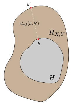
Figure 3: Distance between $H$ and $H_{X,Y}$; see Example 4.18.

To state such a stability result, we first need a way to quantify changes to the predictor set. The most salient aspect of a predictor $h$ is its performance with respect to the chosen loss function. In other words, more crucial than the predictor $h$ itself is the function $\ell_{h}(x,y):=\ell(h(x),y)$. With this perspective in mind, we can map $H$ into $L^{1}(\eta)$ via the map $h\mapsto\ell_{h}$, and compare predictors using the $L^{1}$ norm there. That is, we compare two predictors $h$ and $h^{\prime}$ via the quantity

$$d_{\ell,\eta}(h,h^{\prime}):=\|\ell_{h}-\ell_{h^{\prime}}\|_{L^{1}(\eta)}=\int\big{|}\ell_{h}(x,y)-\ell_{h^{\prime}}(x,y)\big{|}\,\eta(dx{\times}dy).$$

This defines a pseudometric on the set of all measurable functions $h:X\to Y$ for which $\|\ell_{h}\|_{L^{1}(\eta)}<\infty$, which any predictor satisfies since the definition of a problem mandates that predictors have finite risk. The map $h\mapsto\ell_{h}$ identifies two predictors $h$ and $h^{\prime}$ if they $\eta$-almost always incur the same loss on a random observation in $X\times Y$.

We can now state a stability theorem in terms of the Hausdorff distance on predictor sets with underlying metric $d_{\ell,H}$, i.e. the metric

$$d_{\mathrm{H}}^{d_{\ell,\eta}}(H,H^{\prime})=\inf_{R\in{\mathcal{C}}(H,H^{\prime})}\sup_{(h,h^{\prime})\in R}\|\ell_{h}-\ell_{h^{\prime}}\|_{L^{1}(\eta)}.$$

Theorem 4.17.

Let $P$ be a problem, and let $P^{\prime}$ be a problem that is identical to $P$ except possibly for the predictor set $H^{\prime}$. Then

$$d_{\mathrm{R}}(P,P^{\prime})\leq d_{\mathrm{H}}^{d_{\ell,\eta}}\left(H,H^{\prime}\right).$$

Example 4.18.

Note that if $P=(X,Y,\eta,\ell,H)$ and $P^{\prime}=(X,Y,\eta,\ell,H_{X,Y})$, where $H_{X,Y}$ stands for the set of all measurable functions from $X$ to $Y$, Theorem 4.3 implies that

$${\mathcal{B}}^{*}(P)\leq{\mathcal{B}}(P)\leq{\mathcal{B}}^{*}(P)+\sup_{h^{\prime}\in H_{X,Y}}\inf_{h\in H}d_{\ell,\eta}(h,h^{\prime}).$$

The right-hand side contains the worst case $d_{\ell,\eta}$ distance between an arbitrary measurable function $h^{\prime}$ and the (constrained) predictor set $H$. In other words, this quantity expresses how far $H$ is from the superclass $H_{X,Y}$ and therefore controls the approximation error: the difference between the constrained and unconstrained Bayes risks; see Figure 3.

Theorem 4.17.

We bound $d_{\mathrm{R}}(P,P^{\prime})$ by choosing the diagonal coupling between $\eta$ and itself. That is,

$$d_{\mathrm{R}}(P,P^{\prime}) \leq\inf_{R\in{\mathcal{C}}(H,H^{\prime})}\sup_{(h,h^{\prime})\in R}\int\big{|}\ell(h(x),y)-\ell(h^{\prime}(x),y)\big{|}\,\eta(dx{\times}dy)$$

$$=\inf_{R\in{\mathcal{C}}(H,H^{\prime})}\sup_{(h,h^{\prime})\in R}\|\ell_{h}-\ell_{h^{\prime}}\|_{L^{1}(\eta)}=d_{\mathrm{H}}^{d_{\ell,\eta}}(H,H^{\prime}),$$

which is the desired bound. ∎

We illustrate the metric $d_{\mathrm{H}}^{d_{\ell,\eta}}$ and Theorem 4.17 with a toy example.

Example 4.19.

Let $P=({\mathbb{R}}^{2},\{0,1\},\eta,\ell,H)$ be the classification problem from Example 3.5. Recall that the predictors in $H$ were the functions of the form

$$h_{a,b,c}(x_{1},x_{2}):=\begin{cases}1&ax_{1}+bx_{2}\geq c\\ 0&ax_{1}+bx_{2}<c\end{cases}.$$

We modify $H$ by adding to each predictor a small area on which they always predict class 1. That is, we define a new predictor set $H^{\prime}_{t}:=\left\{h^{\prime}_{a,b,c,t}\middle|a,b,c\in{\mathbb{R}}\right\}$ where $h^{\prime}_{a,b,c,t}:{\mathbb{R}}^{2}\to\{0,1\}$ is given by

$$h^{\prime}_{a,b,c,t}(x_{1},x_{2}):=\begin{cases}1&x\in B_{t}(0)\\ h_{a,b,c}(x)&\text{otherwise}\end{cases}.$$

Here $B_{t}(0)$ represents the ball of radius $t$ centered at 0. We can construct a correspondence between $H$ and $H^{\prime}_{t}$ by coupling each $h_{a,b,c}$ with $h^{\prime}_{a,b,c,t}$. That is, we define

$$R:=\left\{(h_{a,b,c},h^{\prime}_{a,b,c,t})\middle|a,b,c\in{\mathbb{R}}\right\}.$$

Then $R\in{\mathcal{C}}(H,H^{\prime}_{t})$, so we can write the bound

$$d_{\mathrm{H}}^{d_{\ell,\eta}}(H,H^{\prime}_{t}) \leq\sup_{(h_{a,b,c},h^{\prime}_{a,b,c,t})\in R}\|\ell_{h_{a,b,c}}-\ell_{h_{a,b,c,t}}\|_{L^{1}(\eta)}$$

$$=\sup_{a,b,c\in{\mathbb{R}}}\int\big{|}\ell(h_{a,b,c}(x),y)-\ell(h_{a,b,c,t}(x),y)\big{|}\,\eta(dx{\times}dy)$$

$$=\sup_{a,b,c\in{\mathbb{R}}}\int_{B_{t}(0)\times\{0,1\}}\big{|}\ell(h_{a,b,c}(x),y)-\ell(h_{a,b,c,t}(x),y)\big{|}\,\eta(dx{\times}dy)$$

$$\leq\eta(B_{t}(0)\times\{0,1\}).$$

Furthermore, assuming $\eta({0}\times\{0,1\})=0$, we can take the limit as $t\to 0$ to get $\lim_{t\to 0}d_{\mathrm{H}}^{d_{\ell,\eta}}(H,H^{\prime}_{t})=0$. If we define $P_{t}:=({\mathbb{R}}^{2},\{0,1\},\eta,\ell,H^{\prime}_{t})$ for all $t>0$, By Theorem 4.17, $P_{t}$ converges to $P$ under the Risk distance as $t\to 0$.

We now provide a more serious application of Theorem 4.17. Different classes of predictors are often compared in the context of universal approximation theorems, which generally state that a certain kind of function can be approximated arbitrarily well using a certain class of model. Using Theorem 4.17, one can translate universal approximation theorems into statements about the risk distance. While there are many universal approximation theorems (Pinkus, 1999), we will demonstrate with a classical example (see Leshno et al., 1993).

Proposition 4.20.

Let $\phi:{\mathbb{R}}\to{\mathbb{R}}$ be a continuous non-polynomial function. Let $P=(X,{\mathbb{R}},\eta,\ell,H)$ be a problem where

• $X$ is a compact subset of ${\mathbb{R}}^{m}$,

• $\eta$ is any probability distribution on $X$,

• $\ell$ is a uniformly continuous loss function, and

• $H$ is the set of all functions $X\to{\mathbb{R}}$ which can come from a feedforward network with a single hidden layer of arbitrary width and with activation function $\phi$. That is, $H$ is the set of all functions of the form

  $$(x_{1},\dots,x_{m})\mapsto\sum_{i=1}^{M}a_{i}\phi\left(\sum_{j=1}^{m}w_{ij}x_{j}+b_{i}\right)$$

  where the parameters $a_{i}$, $w_{ij}$, and $b_{j}$ range over ${\mathbb{R}}$, and $M$ ranges over the positive integers.

Let $P^{\prime}$ be the same problem, but with predictor set $H^{\prime}$ the set of all continuous functions $X\to{\mathbb{R}}$. Then $d_{\mathrm{R}}(P,P^{\prime})=0$.

Proof.

Let $h^{\prime}:X\to{\mathbb{R}}$ be continuous and let $\varepsilon>0$ be arbitrary. By uniform continuity of $\ell$, there exists a $\delta>0$ such that, if $|y-y^{\prime}|<\delta$, then $|\ell(y,y^{\prime\prime})-\ell(y^{\prime},y^{\prime\prime})|<\varepsilon$ for any $y^{\prime\prime}\in{\mathbb{R}}$. By (Leshno et al., 1993, Thm 1), there exists an $h\in H$ with $|h(x)-h^{\prime}(x)|<\delta$ for all $x\in X$. Then

$$d_{\ell,\eta}(h,h^{\prime}) =\int\big{|}\ell(h(x),y)-\ell(h^{\prime}(x),y)\big{|}\,\eta(dx{\times}dy)\leq\int\varepsilon\,\eta(dx{\times}dy)=\varepsilon.$$

Since $H\subseteq H^{\prime}$, this implies the Hausdorff distance $d_{H}^{d_{\ell,\eta}}(H,H^{\prime})$ is less than $\varepsilon$. By Theorem 4.17, $d_{\mathrm{R}}(P,P^{\prime})<\varepsilon$ as well. ∎

In other words, under certain conditions, the risk distance does not distinguish between a model and the class of functions in which it is dense.

5 Geometry of the Space of Problems

We now shift our attention from stability properties of $d_{\mathrm{R}}$ to its geometric properties. We will explore geodesics and their connection to optimal couplings and correspondences. We also show that classification problems (that is, those with finite output spaces) are dense in a larger class of problems. We will use this density to study the effect of limited sampling by studying the convergence of “empirical problems,” which are problems whose joint laws are given by empirical measures gleaned from finite random samples.

Figure 4: A simple depiction of two problem $P$ and $P^{\prime}$ in the space of problems, joined by a geodesic.

5.1 Geodesics

We begin our exploration of the geometry of the space of problems by searching for geodesics. A geodesic in a metric space $(X,d_{X})$ is a continuous function from the unit interval $f:[0,1]\to X$ such that, for all $s,t\in[0,1]$,

$$d_{X}(f(t),f(s))=d_{X}(f(0),f(1))|s-t|.$$

Some would call such an $f$ a “shortest path” (Burago et al., 2001, Chapter 2.5) and reserve the term “geodesic” for a path that locally satisfies the above property. However, the above definition is standard in the field of optimal transport (Ambrosio et al., 2021, Section 9.2, Eq. 9.4).

While valuable in illuminating the geometry of a space, geodesics are not solely of geometric interest. A geodesic between two points gives us a way to interpolate or average between them. If a family $\{P_{t}\}_{t\in[0,1]}$ of problems defines a geodesic in the space of problems, then $P_{1/2}$ could reasonably be considered an average of $P_{0}$ and $P_{1}$. If we would rather take a weighted average, we could choose smaller or larger values of $t$ to give more weight to $P_{0}$ or to $P_{1}$ respectively.

We will show that geodesics can be supplied by certain couplings and correspondences.

Definition 5.1.

Let $P$ and $P^{\prime}$ be problems. If there exists a coupling $\gamma\in\Pi(\eta,\eta^{\prime})$ and a correspondence $R\in{\mathcal{C}}(H,H^{\prime})$ such that

$$d_{\mathrm{R}}(P,P^{\prime})=\operatorname{dis}_{P,P^{\prime}}(R,\gamma),$$

then we call $\gamma$ an optimal coupling and $R$ an optimal correspondence for $P$ and $P^{\prime}$. That is, $\gamma$ and $R$ are called optimal if they achieve the infima in the definition of $d_{\mathrm{R}}(P,P^{\prime})$.

In Section 5.2, we will explore sufficient conditions for the existence of optimal couplings and correspondences. Presently, we motivate our interest in optimal couplings and correspondences by showing that they are closely related to the geometry of the space of problems; optimal couplings and correspondences provide us with explicit geodesics in the space of problems.

Theorem 5.2.

Suppose $P_{0}$ and $P_{1}$ admit an optimal coupling $\gamma$ and an optimal correspondence $R$. Then the following family of problems is a geodesic between $P_{0}$ and $P_{1}$:

$$P_{t}:=(X_{0}\times X_{1},Y_{0}\times Y_{1},\gamma,\ell_{t},R_{\times})$$

for all $t\in[0,1]$, where

• $\ell_{t}((y_{0},y_{1}),(y^{\prime}_{0},y^{\prime}_{1})):=(1-t)\ell_{0}(y_{0},y^{\prime}_{0})+t\ell_{1}(y_{1},y^{\prime}_{1})$.

• $R_{\times}:=\{h_{0}\times h_{1}|h_{0}\in H_{0},h_{1}\in H_{1}\}$.

It may at first appear that we have given $P_{0}$ two conflicting definitions in the above statement, once as the given

$$P_{0}:=(X_{0},Y_{0},\eta_{0},\ell_{0},H_{0})$$

and again by setting $t=0$ in our parameterized family, yielding

$$P_{0}:=(X_{0}\times X_{1},Y_{0}\times Y_{1},\gamma,\ell_{0},R_{\times}).$$

However, the latter problem is a simulation of the former via the projection maps $X_{0}\times X_{1}\to X_{0}$ and $Y_{0}\times Y_{1}\to Y_{0}$. Hence the two problems are distance zero apart under the Risk distance and can be safely identified. A similar line of thought applies to $P_{1}$.

The proof that this family is a geodesic is very similar to the proofs of analogous results for the Gromov-Hausdorff and Gromov-Wasserstein distances (Chowdhury and Mémoli, 2018; Sturm, 2012).

Proof.

Define $C:=d_{\mathrm{R}}(P_{0},P_{1})$. Let $0\leq s\leq t\leq 1$. If we can show

$$d_{\mathrm{R}}(P_{s},P_{t})\leq C(t-s),$$

then equality will follow. Indeed, if the inequality were strict for some $0\leq s_{0}\leq t_{0}\leq 1$, then we could use the triangle inequality to write

$$C=d_{\mathrm{R}}(P_{0},P_{1}) \leq d_{\mathrm{R}}(P_{0},P_{s_{0}})+d_{\mathrm{R}}(P_{s_{0}},P_{t_{0}})+d_{\mathrm{R}}(P_{t_{0}},P_{1})$$

$$<s_{0}C+(t_{0}-s_{0})C+(1-s_{0})C=C,$$

which is a contradiction.

Now, we can bound $d_{\mathrm{R}}(P_{s},P_{t})$ by selecting the diagonal coupling from $\Pi(\gamma,\gamma)$ and diagonal correspondence from ${\mathcal{C}}(R_{\times},R_{\times})$ to get

$$d_{\mathrm{R}}(P_{s},P_{t})$$

$$\leq \sup_{h_{0}\times h_{1}\in R_{\times}}\int\big{|}\ell_{s}((h_{0}(x_{0}),h_{1}(x_{1})),(y_{0},y_{1}))-\ell_{t}((h_{0}(x_{0}),h_{1}(x_{1})),(y_{0},y_{1}))\big{|}\,\gamma(dx_{0}{\times}dy_{0}{\times}dx_{1}{\times}dy_{1})$$

$$= \sup_{h_{0}\times h_{1}\in R_{\times}}\int\big{|}(t-s)\big{(}\ell_{0}(h_{0}(x_{0}),y_{0})+\ell_{1}(h_{1}(x_{1}),y_{1})\big{)}\big{|}\,\gamma(dx_{0}{\times}dy_{0}{\times}dx_{1}{\times}dy_{1})$$

$$=(t-s)\sup_{(h_{0},h_{1})\in R}\int\big{|}\ell_{0}(h_{0}(x_{0}),y_{0})+\ell_{1}(h_{1}(x_{1}),y_{1})\big{|}\,\gamma(dx_{0}{\times}dy_{0}{\times}dx_{1}{\times}dy_{1})$$

$$=(t-s)C.$$

The last equality is because $\gamma$ and $R$ are an optimal coupling and correspondence of $P_{0}$ and $P_{1}$. ∎

5.2 Existence of Optimal Couplings and Correspondences

Motivated by Theorem 5.2, we search for conditions under which optimal couplings and correspondences exist. We will achieve this by imposing some continuity and compactness conditions on our problems.

Definition 5.3.

A problem $P$ is called continuous if, for all $h\in H$, $\ell_{h}$ is continuous $\eta$-almost everywhere.

Note that the above condition applies to many relevant problems. A typical linear regression problem will be continuous. For instance, the linear regression problem in Example 3.6 is continuous, since the loss is continuous, as is every predictor. Under reasonable assumptions, a classification problem can be continuous as well; one only needs the possible decision boundaries to each have measure zero in the $X$-marginal. Take the classification problem $P$ in Example 3.5. In that problem, $\ell_{h}$ is discontinuous for every predictor $h$. However, if we assume that any line in ${\mathbb{R}}^{2}$ has measure zero with respect to the $X$-marginal of $\eta$ (as would be the case if the $X$-marginal of $\eta$ is given by a continuous probability distribution), then any linear decision boundary has measure zero. Consequently, $\ell_{h}$ will be continuous (indeed, constant) $\eta$-almost everywhere.

Let $P,P^{\prime}$ be continuous problems. Recall that the risk distortion is the function

$$\operatorname{dis}_{P,P^{\prime}}:{\mathcal{C}}(H,H^{\prime})\times\Pi(\eta,\eta^{\prime})\to\mathbb{R}$$

$$\operatorname{dis}_{P,P^{\prime}}(R,\gamma):=\sup_{(h,h^{\prime})\in R}\int\big{|}\ell_{h}(x,y)-\ell_{h^{\prime}}(x^{\prime},y^{\prime})\big{|}\,\gamma(dx{\times}dy{\times}dx^{\prime}{\times}dy^{\prime}).$$

We would like to discuss the potential continuity of this function, and hence require a suitable topology on its domain. We endow $\Pi(\eta,\eta^{\prime})$ with the weak topology. We give the set $\left\{\ell_{h}\middle|h\in H\right\}$ the $L^{1}(\eta)$ topology, and endow $H$ with the initial topology induced by the map $h\mapsto\ell_{h}$. Equivalently, we endow $H$ with the pseudometric $d_{\ell,\eta}$ defined in Section 4.5 and similarly equip $H^{\prime}$ with $d_{\ell^{\prime},\eta^{\prime}}$. We then endow $H\times H^{\prime}$ with the product metric $\delta((g,g^{\prime}),(h,h^{\prime})):=\max\{d_{\ell,\eta}(g,h),d_{\ell^{\prime},\eta^{\prime}}(g^{\prime},h^{\prime})\}$, and place the resulting Hausdorff distance $d_{\mathrm{H}}^{\delta}$ on ${\mathcal{C}}(H,H^{\prime})$.

Define

$$\widetilde{\operatorname{dis}}_{P,P^{\prime}}:H\times H^{\prime}\times\Pi(\eta,\eta^{\prime})\to{\mathbb{R}}$$

$$\widetilde{\operatorname{dis}}_{P,P^{\prime}}(h,h^{\prime},\gamma):=\int\big{|}\ell_{h}(x,y)-\ell_{h^{\prime}}(x^{\prime},y^{\prime})\big{|}\,\gamma(dx{\times}dy{\times}dx^{\prime}{\times}dy^{\prime}).$$

Hence

$$\operatorname{dis}_{P,P^{\prime}}(R,\gamma)=\sup_{(h,h^{\prime})\in R}\widetilde{\operatorname{dis}}_{P,P^{\prime}}(h,h^{\prime},\gamma).$$

We proceed with a sequence of lemmas. We begin by showing that, under certain conditions, $\widetilde{\operatorname{dis}}_{P,P^{\prime}}$ is lower semi-continuous, then leverage this result to obtain lower semi-continuity of $\operatorname{dis}_{P,P^{\prime}}$. Recall that a function $f:S\to{\mathbb{R}}$ on a topological space $S$ is lower semi-continuous if, for all $x_{0}\in S$, we have $\liminf_{x\to x_{0}}f(x)\geq f(x_{0})$. Lower semi-continuity is a useful notion because such functions satisfy a limited version of the extreme value theorem. Specifically, a lower semi-continuous function on a compact space achieves its minimum.

Lemma 5.4.

Let $P$ and $P^{\prime}$ be continuous problems. Then $\widetilde{\operatorname{dis}}_{P,P^{\prime}}$ is lower semi-continuous.

Lemma 5.5.

Let $P$ and $P^{\prime}$ be continuous problems. Then $\operatorname{dis}_{P,P^{\prime}}$ is lower semi-continuous.

Using the fact that a lower semi-continuous function on a compact set achieves its minimum, we can prove the following Theorem.

Theorem 5.6.

If $P$ and $P^{\prime}$ are continuous problems with compact predictor sets, then there exists an optimal coupling and correspondence for $P$ and $P^{\prime}$. That is, there exists $R\in{\mathcal{C}}(H,H^{\prime})$ and $\gamma\in\Pi(\eta,\eta^{\prime})$ such that

$$d_{\mathrm{R}}(P,P^{\prime})=\operatorname{dis}_{P,P^{\prime}}(R,\gamma).$$

The proofs can be found in Appendix A. In turn, Theorem 5.6 and the characterization of weak isomorphism provided by Theorem 3.16 give us conditions under which weak isomorphism is equivalent to being Risk distance zero apart.

Corollary 5.7.

If $P$ and $P^{\prime}$ are continuous problems with compact predictor sets, then $P$ and $P^{\prime}$ are weakly isomorphic if and only if $d_{\mathrm{R}}(P,P^{\prime})=0$.

5.3 Density of Classification Problems

One benefit of equipping a set with a pseudometric is that, in return, we receive a notion of convergence. One can ask whether a sequence of points converges, how quickly it does so, and what the limit might be. Density results pave the way for limiting arguments. It is often possible, by a limiting argument, to transfer knowledge about a “simple” dense subspace to the space as a whole.

In this section, we show that classification problems (that is, problems whose output space is a finite collection of labels) are dense in a broader class of functions under $d_{\mathrm{R}}$. We will leverage this information in Section 5.4 to prove the main result of the section: the convergence of empirical problems (Theorem 5.15).

Definition 5.8 (Classification Problem).

A problem is called a classification problem if its response space is finite. A problem is called compact if its response space is compact and its loss function is continuous.

A classification problem is so called because we can think of its response space as a finite collection of labels. In Appendix B, we characterize the problems that are weakly isomorphic to classification problems.

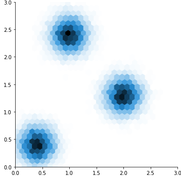
$\qquad\underset{\text{Coarsening}}{\scalebox{4.0}{$\rightsquigarrow$}}\qquad$

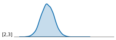
Figure 5: A depiction of the coarsening process in Example 5.10. On the left is a heat map depicting the joint law $\eta$ of a problem $P$ whose input and output spaces are both the interval $X=Y=[0,3]$. We consider the partition $Q=\{[0,1),[1,2),[2,3]\}$ of $Y=[0,3]$. The coarsened problem $P_{Q}:=(X,Q,\eta_{Q},\ell_{Q},H_{Q})$ has three points in the output space $Q$, represented by the vertical axis. The joint law $\eta_{Q}$ is then a probability measure on three copies of $[0,3]$. We depict $\eta_{Q}$ on the right with density plots of the three class-conditional probability measures.

Given a compact problem $P$, we can produce a related classification problem $P_{Q}$ by clustering the response space into a finite partition $Q$ and applying a procedure we call coarsening. The definition of a coarsening makes use of a certain map associated to a partition. Given a set $A$ and a partition $Q$ of $A$, consider the map $\pi_{Q}:A\to Q$ which sends each $a\in A$ to the unique partition block $q\in Q$ which contains $a$. That is, $\pi_{Q}$ is defined such that $a\in\pi_{Q}(a)$ for all $a\in A$. This map $\pi_{Q}$ is often called the quotient map associated to $Q$.

Definition 5.9 (Coarsening).

Let $P$ be a problem, let $Q$ be a finite partition of $Y$ into measurable sets, and let $\pi_{Q}:Y\to Q$ be the quotient map associated to $Q$. The coarsening of $P$ with respect to $Q$ is the classification problem

$$P_{Q}=(X,Q,\eta_{Q},\ell_{Q},H_{Q})$$

where

• $\eta_{Q}:=(\operatorname{Id}_{X}\times\pi_{Q})_{\sharp}\eta$

• $\ell_{Q}(q,q^{\prime}):=\sup_{y\in q,y^{\prime}\in q^{\prime}}\ell(y,y^{\prime})$,

• $H_{Q}:=\left\{\pi_{Q}\circ h\middle|h\in H\right\}$.

Note that if $Q$ is a finite partition of $Y$, then $Q$ is itself a finite set of partition blocks. The response space $Q$ of the coarsened problem $P_{Q}$ is a finite set with one element for each block of the partition $Q$, and hence $P_{Q}$ is indeed a classification problem.

Example 5.10.

An example of the coarsening procedure is depicted in Figure 5. We imagine a problem

$$P=([0,3],[0,3],\eta,\ell,H)$$

where $\eta$ is as pictured, $\ell(y_{1},y_{2}):=|y_{1}-y_{2}|$ is the Euclidean distance, and $H$ is the set of increasing continuous bijections $[0,3]\to[0,3]$. We choose the partition $Q=\{[0,1),[1,2),[2,3]\}$ of $P$ and consider the coarsened problem

$$P_{Q}=([0,3],Q,\eta_{Q},\ell_{Q},H_{Q}).$$

Then $P_{Q}$ is a classification problem with three points in its output space $Q=\{q_{1},q_{2},q_{3}\}$, where $q_{1}:=[0,1),q_{2}:=[1,2),$ and $q_{3}:=[2,3]$. Then $\eta_{Q}$ is a probability measure on $[0,3]\times Q$, a space which consists of three line segments: $[0,3]\times\{q_{1}\}$, $[0,3]\times\{q_{2}\}$, and $[0,3]\times\{q_{3}\}$. The coarsened loss

$$\ell_{Q}(q_{i},q_{j}):=\sup_{y\in q_{i},y^{\prime}\in q_{j}}\ell(y,y^{\prime})\,\,\mbox{for $i,j=1,2,3$},$$

can be written in the form of a table:

$\ell_{Q}$	$q_{1}$	$q_{2}$	$q_{3}$
$q_{1}$	1	2	3
$q_{2}$	2	1	2
$q_{3}$	3	2	1

The predictor set $H_{Q}$ is $\left\{\pi_{Q}\circ h\middle|h\in H\right\}$, where $\pi_{Q}:Y\to Q$ is the quotient map. Then $H_{Q}$ can also be written as the set of all functions $g:[0,3]\to Q$ of the form

$$g(t)=\begin{cases}q_{1}&t<a\\ q_{2}&a\leq t<b\\ q_{3}&b\leq t\end{cases}$$

for all $0<a\leq b<3$.

Coarsening is reminiscent of the “probing reduction” (Langford and Zadrozny, 2005), which takes a probability estimation problem and solves it with an ensemble of classifier learners, hence “reducing” the problem of probability estimation to the problem of binary classification. Indeed, one can view the probing reduction as a practical method of approximating a problem whose output space is $Y=[0,1]$ by iteratively constructing finer and finer partitions of $Y$ and solving the resulting coarsened problems with binary classifiers.

Theorem 5.11.

Let $P$ be a compact problem. For any $\varepsilon>0$, there is a partition $Q$ of the response space such that

$$d_{\mathrm{R}}(P,P_{Q})<\varepsilon.$$

The proof is relegated to Appendix A.

Remark 5.12.

One notable feature of the proof of Theorem 5.11 is that the partition $Q$ provided by the theorem does not depend on the joint law $\eta$ of $P$. More precisely, suppose $P$ is a problem. For any probability measure $\eta^{\prime}\in\operatorname{Prob}(X\times Y)$, we can create a new problem

$$P_{\eta^{\prime}}:=(X,Y,\eta^{\prime},\ell,H).$$

The proof of Theorem 5.11 shows that, not only can we find a partition $Q$ of $Y$ such that $d_{\mathrm{R}}(P,P_{Q})<\varepsilon$, but we can choose $Q$ such that for all $\eta^{\prime}\in\operatorname{Prob}(X\times Y)$, we have $d_{\mathrm{R}}((P_{\eta^{\prime}})_{Q},P_{\eta^{\prime}})<\varepsilon$. We will use this stronger fact to prove Theorem 5.15.

Theorem 5.11 immediately gives us a density result.

Corollary 5.13 (Classification Density Theorem).

Under $d_{\mathrm{R}}$, the set of classification problems is dense in the space of compact problems.

5.4 Convergence of Empirical Problems

With the density of classification problems in hand, we are ready to examine the effect that limited sampling can have on a problem. One often does not have direct knowledge of the underlying joint law from which data is sampled; one only has access to a finite data set. In terms of our supervised learning problems, instead of accessing the joint law $\eta$ of a problem $P$ directly, we can only access the empirical measure $\eta_{n}$ of $\eta$. Namely, given an i.i.d. set $\{(x_{i},y_{i})\}_{i=1}^{n}$ sampled from the probability measure $\eta$, we set

$$\eta_{n}:=\frac{1}{n}\sum_{i=1}^{n}\delta_{(x_{i},y_{i})}.$$

The resulting problem with joint law $\eta_{n}$ is called the empirical problem.

Definition 5.14.

If $P$ is a problem, the $n$th empirical problem induced by $P$ is the random problem defined by

$$P_{n}:=(X,Y,\eta_{n},\ell,H).$$

Being dependent on a random sample, $\eta_{n}$ is a random measure. Consequently, $P_{n}$ is a random problem. One would hope that as the size of the sample grows, the empirical problem $P_{n}$ converges to the true problem $P$ with probability 1. Under certain conditions, this is indeed true.

Theorem 5.15 (Convergence of the Empirical Problem).

Let $P$ be a problem satisfying the following:

1. $H$ is compact with respect to $d_{\ell,\eta}$.

2. $Y$ is compact.

3. $\ell$ is continuous.

4. The collection $\{|\ell_{h}-\ell_{h^{\prime}}|\}_{h,h^{\prime}\in H}$ forms a Glivenko-Cantelli class with respect to $\eta$.

Let $P_{n}$ be the $n$th empirical problem induced by $P$. Then $d_{\mathrm{R}}(P,P_{n})\to 0$ almost surely.

The proof, found in Appendix A, uses Theorem 5.11 to reduce to the case where $P$ is a classification problem. We briefly illuminate the Glivenko-Cantelli condition in Theorem 5.15 by providing simpler sufficient conditions.

Proposition 5.16.

Define $g_{h,h^{\prime}}(x,y):=|\ell_{h}(x,y)-\ell_{h^{\prime}}(x,y)|$. Theorem 5.15 still holds if Condition 4 is replaced with either of the following conditions.

1. The collection of subgraphs $\left\{\mathrm{sg}(g_{h,h^{\prime}})\middle|h,h^{\prime}\in H\right\}$ (see Definition 2.11) has finite VC dimension.

2. For any $h_{0},h^{\prime}_{0}\in H$ and $\varepsilon>0$, there exists an open neighborhood $(h_{0},h^{\prime}_{0})\in U\subseteq H\times H$ such that

   $$\int\sup_{(h,h^{\prime})\in U}g_{h,h^{\prime}}(x,y)\eta(dx{\times}dy)-\varepsilon <\int g_{h_{0},h^{\prime}_{0}}(x,y)\eta(dx{\times}dy)<\int\inf_{(h,h^{\prime})\in U}g_{h,h^{\prime}}(x,y)\eta(dx{\times}dy)+\varepsilon.$$

Conditions 2 and 4a together imply condition 4, since the compactness of $Y$ implies that the $g_{h,h^{\prime}}$ are uniformly bounded, and hence that Proposition 2.12 applies. Note that Condition 4a does not depend on the joint law $\eta$. Conditions 1 and 4b together imply condition 4 as well by a theorem of Gaenssler (1975).

6 The $L^{p}$-Risk Distance: Weighting Problems

In this section we introduce a variant of the Risk distance called the $L^{p}$-Risk distance which incorporates probability measures on the predictor sets. This additional information lets us prioritize certain predictors over others by weighting them more heavily, subsequently softening the Risk distance and improving its stability.

6.1 Weighting Predictor Sets and the $L^{p}$-Risk Distance

Many of our results thus far have required assumptions of compact predictor sets or bounded loss functions. Without these assumptions, the Risk distance tends to be poorly-behaved. For instance, problems such as the linear regression in Example 3.6 tend to be infinitely far away from problems of bounded loss under the Risk distance. One reason for this phenomenon is the supremum in the definition of the Risk distance. The supremum treats unreasonable predictors, such as those whose graphs are far from the support of the joint law, with the same consideration as more reasonable options. One might reasonably complain about this design decision.

One solution to this problem is to weight the predictors, de-prioritizing extreme options by giving them less weight. These weights could come from prior knowledge or belief about which predictors might perform well or from a measure of complexity of each predictor (so that more complex predictors receive lower weights). Indeed, considering these weights as part of the specification of a problem can be seen as a proxy for adding regularization term to the constrained Bayes risk.

More formally, we provide weights on the predictor set in the form of a probability measure. This lets us replace the supremum in the definition of $d_{\mathrm{R}}$ with an $L^{p}$-type integral, effectively softening the Risk distance.

Definition 6.1.

A weighted problem is a pair $(P,\lambda)$ where

• $P$ is a problem whose predictor set $H$ comes equipped with a Polish topology, and

• $\lambda$ is a probability measure on $H$.

When there is no chance of confusion, we may suppress the measure $\lambda$ and denote the weighted problem by $P$.

Assumption 6.2.

We make the following measurability assumption. Given a weighted problem $(P,\lambda)$, consider the map

$$H\times X\times Y \to{\mathbb{R}}_{\geq 0}$$

given by

$$(h,x,y) \mapsto\ell_{h}(x,y).$$

Since $H$, $X$, and $Y$ are topological spaces, we can equip each space with the corresponding Borel $\sigma$-algebra. We can then equip the product $H\times X\times Y$ with the product $\sigma$-algebra. For any weighted problem $(P,\lambda)$, we henceforth assume that the above map $(h,x,y)\mapsto\ell_{h}(x,y)$ is measurable with respect to this product $\sigma$-algebra.

Definition 6.3.

Let $(P,\lambda)$ and $(P^{\prime},\lambda^{\prime})$ be weighted problems. For $p\in[1,\infty]$ and for any couplings $\gamma\in\Pi(\eta,\eta^{\prime})$ and $\rho\in\Pi(\lambda,\lambda^{\prime})$, define the $L^{p}$-risk distortion of $\gamma$ and $\rho$ to be

$$\operatorname{dis}_{P,P^{\prime},p}(\rho,\gamma) :=\left(\int\left(\int\big{|}\ell(h(x),y)-\ell^{\prime}(h^{\prime}(x^{\prime}),y^{\prime})\big{|}\,d\gamma(x,y,x^{\prime},y^{\prime})\right)^{p}d\rho(h,h^{\prime})\right)^{1/p} p\in[1,\infty)$$ ,

$$\operatorname{dis}_{P,P^{\prime},\infty}(\rho,\gamma) :=\sup_{(h,h^{\prime})\in\mathrm{supp}[\rho]}\int\big{|}\ell(h(x),y)-\ell^{\prime}(h^{\prime}(x^{\prime}),y^{\prime})\big{|}\,d\gamma(x,y,x^{\prime},y^{\prime}) p=\infty$$ .

The $L^{p}$-Risk distance between weighted problems $(P,\lambda)$ and $(P^{\prime},\lambda^{\prime})$ is then defined to be

$$d_{\mathrm{R},p}((P,\lambda),(P^{\prime},\lambda^{\prime})) :=\inf_{\rho,\gamma}\operatorname{dis}_{P,P^{\prime},p}(\rho,\gamma)$$

where $\gamma$ ranges over all couplings $\Pi(\eta,\eta^{\prime})$ and $\rho$ ranges over all couplings $\Pi(\lambda,\lambda^{\prime})$.

Theorem 6.4.

The $L^{p}$-Risk distance is a pseudometric on the collection of all weighted problems. Furthermore, we have

• $d_{\mathrm{R},p}\leq d_{\mathrm{R},q}\leq d_{\mathrm{R},\infty}$ for all $1\leq p\leq q\leq\infty$;

• $d_{\mathrm{R}}\leq d_{\mathrm{R},\infty}$.

Remark 6.5.

Property (i) is analogous to a similar property enjoyed by the Gromov-Wasserstein distance (Mémoli, 2011, Theorem 5.1 (h)) and it follows from (Mémoli, 2011, Lemma 2.2). Property (ii) states that the $L^{\infty}$-Risk distance is never smaller than the standard Risk distance from Definition 3.13. This is analogous to the fact that the Gromov-Hausdorff distance is bounded above by the $L^{\infty}$-Gromov-Wasserstein distance (Mémoli, 2011, Theorem 5.1 (b)). The proof of the triangle inequality for the $L^{p}$-Risk distance is identical to the proof of the same for the Risk distance, save for an application of Minkowski’s inequality for the outer integral. As indicated above, the proof of the other claimed properties follows similar steps as those for the Gromov-Wasserstein distance and therefore we omit them.

Example 6.6.

Just as we defined the one-point problems

$$P_{\bullet}(c):=(\{\bullet\},\{\bullet\},\delta_{(\bullet,\bullet)},c,\{\operatorname{Id}_{\{\bullet\}}\})$$

for each $c\geq 0$ in Example 3.7, we can define a corresponding one-point weighted problem by endowing $\{\operatorname{Id}_{\{\bullet\}}\}$ with the point-mass probability measure. We will still use $P_{\bullet}$ to denote $P_{\bullet}(0)$. Then, in a manner similar to Example 3.18, if $(P,\lambda)$ is a weighted problem, one can show

$$d_{\mathrm{R},p}(P,P_{\bullet})=\left(\int_{H}\left(\int_{X\times Y}\ell(h(x),y)\,\eta(dx\times dy)\right)^{p}\,\lambda(dh)\right)^{1/p}=\left(\int_{H}{\mathcal{R}}_{P}^{p}(h)\,\lambda(dh)\right)^{1/p}.$$

This can be seen as a kind of weighted constrained Bayes risk of $(P,\lambda)$. While the constrained Bayes risk of an unweighted problem $P$ is the infimal possible risk, the above expression $d_{\mathrm{R},p}(P,P_{\bullet})$ represents the $p$th moment of possible risks when a predictor is chosen at random according to $\lambda$. In particular, $d_{\mathrm{R},1}(P,P_{\bullet})$ is simply the average risk of a predictor chosen randomly according to $\lambda$.

One can establish a connection with the usual constrained Bayes risk as follows. Assume that the problem $P$ is such that its loss function $\ell$ is bounded above by a constant $\ell_{\max}>0$. Then,

$$d_{\mathrm{R},p}(P,P_{\bullet}(\ell_{\max}))=\left(\int_{H}\big{(}\ell_{\max}-{\mathcal{R}}_{P}(h)\big{)}^{p}\lambda(dh)\right)^{1/p}.$$

If the support of $\lambda$ is the whole $H$, we obtain, as $p\to\infty$, that $d_{\mathrm{R},p}(P,P_{\bullet}(\ell_{\max}))\to\ell_{\max}-{\mathcal{B}}(P).$

The distance $d_{\mathrm{R},p}(P,P_{\bullet})$ from Example 6.6 will appear again in Theorem 6.11, so we establish a definition.

Definition 6.7.

Given a weighted problem $P=(P,\lambda)$ and $1\leq p<\infty$, the $p$-diameter of $P$ is given by

$$d_{\mathrm{R},p}(P,P_{\bullet})=\left(\int_{H}\left(\int_{X\times Y}\ell(h(x),y)\,\eta(dx\times dy)\right)^{p}\,\lambda(dh)\right)^{1/p}=\left(\int_{H}{\mathcal{R}}_{P}^{p}(h)\,\lambda(dh)\right)^{1/p}.$$

The word “diameter” is chosen in analogy with metric geometry, where the diameter of a metric space can be found from its Gromov-Hausdorff distance from the one-point metric space.

6.2 Connection to the Gromov-Wasserstein Distance

In Section 3.5, we saw two ways to turn metric measure spaces into problems, each of which relates the Gromov-Wasserstein distance to the Risk distance. In this section, we will draw a similar connection between the Gromov-Wasserstein distance and the $L^{p}$-Risk distance. Specifically, we will provide a way of turning metric measure spaces into weighted problems such that the $L^{1}$-Risk distance between the resulting problems aligns with a well-known modification of the Gromov-Wasserstein distance between the original spaces.

Given any metric measure space $(X,d_{X},\mu_{X})$, define a weighted problem $(P_{X},\mu_{X})$,

$$P_{X}:=(X,X,(\Delta_{X})_{\sharp}\mu_{X},d_{X},H_{X}),$$

where

• $\Delta_{X}:X\to X\times X$ is the diagonal map $x\mapsto(x,x)$, and

• $H_{X}$ is the set of all constant functions $X\to X$.

Here we think of $\mu_{X}$ as a measure on both $X$ and $H_{X}$ since the two are in natural bijection.

Proposition 6.8.

Let $(X,d_{X},\mu_{X})$ and $(Y,d_{Y},\mu_{Y})$ be two metric measure spaces. Then,

$$d_{\mathrm{R},1}(P_{X},P_{Y})=\inf_{\begin{subarray}{c}\gamma\in\Pi(\mu_{X},\mu_{Y})\\ \rho\in\Pi(\mu_{X},\mu_{Y})\end{subarray}}\int\int\big{|}d_{X}(x_{2},x_{1})-d_{Y}(y_{2},y_{1})\big{|}\,\gamma(dx_{1}{\times}dy_{1})\,\rho(dx_{2}{\times}dy_{2}). \star$$ ()

The proof of this proposition can be found in Appendix A.

Use ${\mathcal{F}}(\gamma,\rho)$ to denote the double integral in the expression ($\star$ ‣ 6.8). If we add the additional constraint that $\gamma=\rho$, then the expression ($\star$ ‣ 6.8) becomes $2d_{\mathrm{GW},1}(X,Y)$. As written, ($\star$ ‣ 6.8) is a lower bound on $2d_{\mathrm{GW},1}(X,Y)$, which could be arrived at via a “bilinear relaxation” of the optimization problem posed by $d_{\mathrm{GW},1}$. That is, one could begin with the objective function for the Gromov-Wasserstein optimization problem

$${\mathcal{F}}^{\prime}(\gamma):=\int\int\big{|}d_{X}(x_{2},x_{1})-d_{Y}(y_{2},y_{1})\big{|}\,\gamma(dx_{1}{\times}dy_{1})\,\gamma(dx_{2}{\times}dy_{2}),$$

which is quadratic in the transport plan $\gamma$, and decouple the two instances of $\gamma$ to get the objective ${\mathcal{F}}(\gamma,\rho)$, which is bilinear in two transport plans. This “relaxation” was considered by (Mémoli, 2011, Section 7) for estimating the Gromov-Wasserstein distance via an alternate minimization procedure. Similar optimal transport problems, which simultaneously optimize two transport plans in a Gromov-Wasserstein-like objective function, appear in the literature. Indeed, when $X$ and $Y$ are finite, the expression ($\star$ ‣ 6.8) is a special case of CO-Optimal transport (Vayer et al., 2020b). Sejourne et al. (2021) apply this relaxation technique, which they call the “biconvex relaxation,” to an unbalanced variant of the Gromov-Wasserstein distance. This inspired Beier et al. (2023) to explore a similar relaxation for a “multi-marginal” variant of the same problem. A theoretical study of the metric properties of the right-hand side of ($\star$ ‣ 6.8) appears in (Chen et al., 2022, Appendix A.4).

6.3 Stability of Loss Profile Distribution

Being softer than the Risk distance, the loss profile is less stable under the $L^{p}$-Risk distance. To obtain a stability result, one cannot compare the loss profile sets directly, but instead compare certain probability distributions on the loss profile sets.

Definition 6.9.

Let $(P,\lambda)$ be a weighted problem. Define $F_{P}:H\to\mathbb{\operatorname{Prob}}({\mathbb{R}})$ by

$$F_{P}(h):=(\ell_{h})_{\sharp}\eta.$$

The loss profile distribution of $P$ is then defined to be ${\mathcal{L}}(P):=(F_{P})_{\sharp}\lambda$.

Note that ${\mathcal{L}}(P)\in\operatorname{Prob}(\operatorname{Prob}({\mathbb{R}}))$ is a probability measure on the space of real probability measures. More specifically, $F_{P}(h)$ is the loss profile of $h$, so ${\mathcal{L}}(P)$ describes what the loss profile of a random predictor chosen according to $\lambda$ is likely to be.

While Theorem 4.3 shows that $L(P)$ is stable under the Risk distance with respect to the Hausdorff distance, the following analogous theorem shows that the measure ${\mathcal{L}}(P)$ is stable under the $L^{p}$-Risk distance with respect to the Wasserstein distance.

Theorem 6.10.

Let $P$ and $P^{\prime}$ be weighted problems. Then

$$d_{\mathrm{W},p}^{d_{\mathrm{W},1}}({\mathcal{L}}(P),{\mathcal{L}}(P^{\prime}))\leq d_{\mathrm{R},p}(P,P^{\prime})$$

where $d_{\mathrm{W},p}^{d_{\mathrm{W},1}}$ is the $p$-Wasserstein metric on $\operatorname{Prob}(\operatorname{Prob}({\mathbb{R}}))$ with underlying metric $d_{\mathrm{W},1}$ on $\operatorname{Prob}({\mathbb{R}})$.

The proof is in Appendix A.

6.4 Improved Density

A useful theorem in measure theory states that any probability measure $\mu$ on a Polish space $X$ is tight, meaning that for any $\varepsilon>0$, there is a compact subset $K\subseteq X$ with $\mu(K)>1-\varepsilon$. In a slogan, “Polish probability spaces are almost compact.” Applying this principle to our setting suggests that any weighted problem should be close to one with a compact predictor set. This can be made rigorous with a density theorem.

Theorem 6.11.

Let $p\geq 1$ and let $(P,\lambda)$ be a weighted problem of finite $p$-diameter. Then there exists a compact weighted problem $(P^{\prime},\lambda^{\prime})$ with $d_{\mathrm{R},p}(P,P^{\prime})<\varepsilon$.

Additionally, a result analogous to Theorem 5.11 still holds for the $L^{p}$-Risk distance.

Proposition 6.12.

Let $p\geq 1$ and let $(P,\lambda)$ be a compact weighted problem. Then there exists a weighted classification problem $(P^{\prime},\lambda^{\prime})$ with $d_{\mathrm{R},p}(P,P^{\prime})<\varepsilon$.

The proofs of both Theorem 6.11 and Proposition 6.12 can be found in Appendix A. Chaining these two density results together proves the following corollary.

Corollary 6.13.

Under $d_{\mathrm{R},p}$ for $p\geq 1$, weighted classification problems are dense in the space of weighted problems of finite $p$-diameter.

Example 6.14.

Consider the linear regression problem $P$ from Example 3.6. If we endow the predictor set of $P$ with a joint law satisfying some finite moment assumptions, the resulting weighted problem has finite $p$-diameter. Corollary 6.13 then tells us that $P$ can be approximated arbitrarily well by weighted classification problems under $d_{\mathrm{R},p}$.

More precisely, let $P$ be a linear regression problem, and suppose the predictor set

$$H=\left\{x\mapsto a^{T}x+b\,\middle|\,(a,b)\in{\mathbb{R}}^{n}\times{\mathbb{R}}\right\}$$

is equipped with a probability measure $\lambda$. We can think of both $\lambda$ and $\eta$ as probability measures on ${\mathbb{R}}^{n}\times{\mathbb{R}}$. If

1. all $n+1$ marginals of $\eta$ have finite second moment, and

2. all $n+1$ marginals of $\lambda$ have finite $2p$-th moment,

then $\operatorname{diam}_{p}(P)<\infty$.

To prove this, we can write

$$\big{(}\operatorname{diam}_{p}(P)\big{)}^{1/2} =\left(\int\left(\int\ell(a^{T}x+b,y)\,\eta(dx\times dy)\right)^{p}\,\lambda(da\times db)\right)^{1/2p}$$

$$=\left(\int\left(\left(\int(a^{T}x+b-y)^{2}\,\eta(dx\times dy)\right)^{1/2}\right)^{2p}\,\lambda(da\times db)\right)^{1/2p}.$$

By liberally applying Minkowski’s inequality and simplifying, we can bound this expression by the sum

$$\sum_{i=1}^{n}\left(\int a_{i}^{2p}\,\lambda(da\times db)\right)^{1/2p}\left(\int x_{i}^{2}\,\eta(dx\times dy)\right)^{1/2}$$

$$+ \left(\int\left(b\right)^{2p}\,\lambda(da\times db)\right)^{1/2p}+\left(\int y^{2}\,\eta(dx\times dy)\right)^{1/2}.$$

These integrals are the moments of $\eta$ and $\lambda$ that we have assumed to be finite.

6.5 Improved Stability

The $L^{p}$-Risk distance enjoys many of the same stability and density results as the Risk distance. Indeed, we will soon see that many of these results can be strengthened for the $L^{p}$-Risk distance. That is, the $L^{p}$-Risk distance enjoys stronger stability and density properties than the Risk distance.

First we will establish that the $L^{p}$-Risk distance inherits some stability results from the Risk distance, saving the improvements for later. Many of our bounds on the Risk distance are proven using the bound

$$d_{\mathrm{R}}(P,P^{\prime})\leq\inf_{\gamma\in\Pi(\eta,\eta^{\prime})}\operatorname{dis}_{P,P^{\prime}}(R_{\mathrm{diag}},\gamma)$$

where $R_{\mathrm{diag}}$ is the diagonal correspondence, which is valid whenever $P$ and $P^{\prime}$ share a predictor set. Hence we can extend the results of those sections using the following lemma.

Lemma 6.15.

Let $(P,\lambda)$ and $(P^{\prime},\lambda)$ be weighted problems that share a predictor set $H$ and predictor weights $\lambda$. Then

$$d_{\mathrm{R},p}((P,\lambda),(P^{\prime},\lambda))\leq\inf_{\gamma\in\Pi(\eta,\eta^{\prime})}\operatorname{dis}_{P,P^{\prime}}(R_{\mathrm{diag}},\gamma)$$

where $R_{\mathrm{diag}}$ is the diagonal correspondence of $H$ with itself.

Proof.

First write

$$d_{\mathrm{R},p}((P,\lambda),(P^{\prime},\lambda))\leq\operatorname{dis}_{P,P^{\prime},p}(\rho_{\mathrm{diag}},\gamma)$$

where $\rho_{\mathrm{diag}}$ is the diagonal coupling of $\lambda$ with itself. Next we bound the $L^{p}$-risk distortion by the $L^{\infty}$-risk distortion as follows:

$$\operatorname{dis}_{P,P^{\prime},p}(\rho_{\mathrm{diag}},\gamma) \leq\operatorname{dis}_{P,P^{\prime},\infty}(\rho_{\mathrm{diag}},\gamma)$$

$$=\sup_{(h,h^{\prime})\in\mathrm{supp}{[\rho_{\mathrm{diag}}}]}\int\big{|}\ell(h(x),y)-\ell^{\prime}(h^{\prime}(x^{\prime}),y^{\prime})\big{|}\,d\gamma(x,y,x^{\prime},y^{\prime})$$

$$\leq\sup_{(h,h^{\prime})\in R_{\mathrm{diag}}}\int\big{|}\ell(h(x),y)-\ell^{\prime}(h^{\prime}(x^{\prime}),y^{\prime})\big{|}\,d\gamma(x,y,x^{\prime},y^{\prime})$$

$$=\operatorname{dis}_{P,P^{\prime}}(R_{\mathrm{diag}},\gamma),$$

where the second inequality follows from the fact that the support of $\rho_{\mathrm{diag}}$ lies within the diagonal $R_{\mathrm{diag}}\subseteq H\times H$. ∎

Condition 2 from Theorem 3.15, the Risk distance bounds of Sections 4.3 (Stability under bias), 4.4 (Stability under noise), and 5.4 (Convergence of empirical problems) are all proven via the diagonal bound (6.5). By Lemma 6.15, these results still hold if we replace the Risk distance with the $L^{p}$-Risk distance and replace both problems with weighted problems that share a common weight measure $\lambda$. That is, in the above results, we can replace each instance of $d_{\mathrm{R}}(P,P^{\prime})$ with $d_{\mathrm{R},p}((P,\lambda),(P^{\prime},\lambda))$ and they will still hold true.

Moreover, some of our results for the Risk distance can be strengthened for the $L^{p}$-Risk distance. Indeed, we have already seen that the density results of Section 5.3 can be strengthened into Theorem 6.11. We can strengthen some stability results in the same manner. For instance, the $L^{p}$-Risk distance satisfies the following version of Condition 2 in which the supremum is replaced by an integral.

Proposition 6.16.

Let $(P,\lambda)$ and $(P^{\prime},\lambda)$ be weighted problems with

$$P =(X,Y,\eta,\ell,H)$$

$$P^{\prime} =(X,Y,\eta,\ell^{\prime},H)$$

Then

$$d_{\mathrm{R},p}(P,P^{\prime})\leq\left(\int\left(\int\big{|}\ell(h(x),y)-\ell^{\prime}(h(x),y)\big{|}\,\eta(dx{\times}dy)\,\right)^{p}\lambda(dh)\right)^{1/p}.$$

Proof.

Bound the $L^{p}$-Risk distance by selecting the diagonal couplings. ∎

We can also modify Theorem 4.17 by replacing the Hausdorff distance with a Wasserstein distance.

Proposition 6.17.

Let $(P,\lambda)$ and $(P,\lambda^{\prime})$ be weighted problems with

$$P :=(X,Y,\eta,\ell,H)$$

$$P^{\prime} :=(X,Y,\eta,\ell,H^{\prime}).$$

Let $i:H\to H\cup H^{\prime}$ and $j:H^{\prime}\to H\cup H^{\prime}$ be the inclusion maps, and endow $H\cup H^{\prime}$ with the pseudometric $d_{\ell,\eta}(h_{1},h_{2}):=\|\ell_{h_{1}}-\ell_{h_{2}}\|_{L^{1}(\eta)}$ introduced in Section 5.2.

Then

$$d_{\mathrm{R},p}(P,P^{\prime})\leq d_{\mathrm{W},p}^{d_{\ell,\eta}}(i_{\sharp}\lambda,j_{\sharp}\lambda^{\prime}).$$

Proof.

Selecting the diagonal coupling between $\eta$ and itself gives us the bound

$$d_{\mathrm{R},p}(P,P^{\prime}) \leq\inf_{\rho\in\Pi(\lambda,\lambda^{\prime})}\left(\int\left(\int\big{|}\ell_{h}(x,y)-\ell_{h^{\prime}}(x,y)\big{|}\,\eta(dx{\times}dy)\right)^{p}\rho(dh{\times}dh^{\prime})\right)^{1/p}$$

$$=\inf_{\rho\in\Pi(i_{\sharp}\lambda,j_{\sharp}\lambda^{\prime})}\left(\int\left(\int\big{|}\ell_{h}(x,y)-\ell_{h^{\prime}}(x,y)\big{|}\,\eta(dx{\times}dy)\right)^{p}\rho(dh{\times}dh^{\prime})\right)^{1/p}$$

$$=\inf_{\rho\in\Pi(i_{\sharp}\lambda,j_{\sharp}\lambda^{\prime})}\left(\int\left(d_{\ell,\eta}(h,h^{\prime})\right)^{p}\rho(dh{\times}dh^{\prime})\right)^{1/p}=d_{\mathrm{W},p}^{d_{\ell,\eta}}(i_{\sharp}\lambda,j_{\sharp}\lambda^{\prime})$$

as desired. ∎

Proposition 4.10 can be modified for weighted problems as well. We first construct an analog of the metric $s_{\ell,H}$ from Section 4.3. Replacing the supremum over $H$ in the definition of $s_{\ell,H}$ with an $L^{p}$-style integral against $\lambda$, we arrive at the definition

$$s_{\ell,\lambda,p}((x,y),(x^{\prime},y^{\prime})):= \left(\int_{H}\big{|}\ell(h(x),y)-\ell(h(x^{\prime}),y^{\prime})\big{|}^{p}\,\lambda(dh)\right)^{1/p}.$$

In other words, to determine the distance between $(x,y)$ and $(x^{\prime},y^{\prime})$, we ask how different the loss on the observation $(x,y)$ will be from the loss on $(x^{\prime},y^{\prime})$ for an average predictor. We can now state our stability result.

Proposition 6.18.

Let $(P,\lambda)$ be a weighted problem, and let $(P^{\prime},\lambda)$ be a weighted problem that is identical to $P$ except possibly for its joint law $\eta^{\prime}$. Then

$$d_{\mathrm{R},p}(P,P^{\prime})\leq d_{\mathrm{W},1}^{s_{\ell,\lambda,p}}(\eta,\eta^{\prime}).$$

Proof.

By selecting the diagonal coupling between $\lambda$ and itself and applying Minkowski’s inequality for integrals, we can bound $d_{\mathrm{R},p}$ by

$$d_{\mathrm{R},p}(P,P^{\prime}) \leq\inf_{\gamma\in\Pi(\eta,\eta^{\prime})}\left(\int\left(\int\big{|}\ell(h(x),y)-\ell(h(x^{\prime}),y^{\prime})\big{|}\,\gamma(dx{\times}dy{\times}dx^{\prime}{\times}dy^{\prime})\right)^{p}\lambda(dh)\right)^{1/p}$$

$$\leq\inf_{\gamma\in\Pi(\eta,\eta^{\prime})}\int\left(\int\big{|}\ell(h(x),y)-\ell(h(x^{\prime}),y^{\prime})\big{|}^{p}\,\lambda(dh)\right)^{1/p}\gamma(dx{\times}dy{\times}dx^{\prime}{\times}dy^{\prime})$$

$$=d_{\mathrm{W},1}^{s_{\ell,\lambda,p}}(\eta,\eta^{\prime}),$$

giving us the desired bound. ∎

Lastly, we turn our attention to stability under noise. We have shown in Section 4.4 that the Risk distance is stable with respect to noise in the joint law when $\ell$ is a metric. By contrast, for a general $\ell$, the Risk distance $d_{\mathrm{R}}$ can be highly sensitive to changes in the joint law. The following example demonstrates this sensitivity.

Example 6.19.

Define a problem

$$P=(\{\bullet\},\mathbb{R},\delta_{0},\ell,H)$$

where $\ell(y,y^{\prime})=(y-y^{\prime})^{2}$, and $H$ is the collection of all functions $\{\bullet\}\to\mathbb{R}$, making $H$ itself homeomorphic to $\mathbb{R}$. Now, for any $\varepsilon>0$, define

$$P_{\varepsilon}=\left(\{\bullet\},\mathbb{R},\frac{1}{2}(\delta_{0}+\delta_{\varepsilon}),\ell,H\right).$$

We can think of $P_{\varepsilon}$ as $P$ with some noise; when making an observation, there is a 50% of observing the correct $y$-value of 0, and a 50% chance of making a small error and reading a $y$-value of $\varepsilon$. We would hope that $P_{\varepsilon}$ would converge to $P$ under $d_{\mathrm{R}}$ as $\varepsilon\to 0$, but this is not true. There is only one coupling between $\delta_{0}$ and $1/2(\delta_{0}+\delta_{\varepsilon})$, so the Risk distance is

$$d_{\mathrm{R}}(P,P_{\varepsilon}) =\inf_{R\in{\mathcal{C}}(H,H)}\sup_{(a,b)\in R}\int\int\big{|}(a-y)^{2}-(b-y^{\prime})^{2}|\,\delta_{0}(dy)\left(\frac{1}{2}\delta_{0}+\frac{1}{2}\delta_{\varepsilon}\right)(dy^{\prime})$$

$$=\inf_{R\in{\mathcal{C}}(H,H)}\sup_{(a,b)\in R}\left[\frac{1}{2}\big{|}a^{2}-b^{2}\big{|}+\frac{1}{2}\big{|}a^{2}-(b-\varepsilon)^{2}\big{|}\right]$$

$$\geq\frac{1}{2}\inf_{R\in{\mathcal{C}}(H,H)}\sup_{(a,b)\in R}\big{|}b^{2}-(b-\varepsilon)^{2}\big{|}$$

$$=\frac{1}{2}\sup_{b\in\mathbb{R}}|2b\varepsilon-\varepsilon^{2}|=\infty.$$

The metric $d_{\mathrm{R},p}$ enjoys a stronger stability than $d_{\mathrm{R}}$ with respect to noise in a problem’s joint law. We use a more general noise model than the one outlined in Section 4.4, allowing for noise in the $X$ direction as well as the $Y$ direction. More specifically, we let our noise be given by any Markov kernel $N:X\times Y\to\operatorname{Prob}(X\times Y)$. That is, given a problem $P$, define $P_{N}$ to be the same problem but with joint law on $X\times Y$ given by

$$\eta\cdot N(A):=\int_{X\times Y}N(x,y)(A)\,\eta(dx\times dy)$$

for all measurable $A\subseteq X\times Y$. We justify the use of Markov kernel composition notation by thinking of the measure $\eta$ as a Markov kernel $\eta:\{\bullet\}\to\operatorname{Prob}(X\times Y)$.

We can now state our improved result about stability under noise.

Theorem 6.20.

Let $(P,\lambda)$ be a weighted problem, and $N:X\times Y\to\operatorname{Prob}(X\times Y)$ a Markov kernel. Then

$$d_{\mathrm{R},p}(P,P_{N})\leq d_{\mathrm{W},1}^{s_{\ell,\lambda,p}}(\delta_{\operatorname{Id}_{X\times Y}},N).$$

Here $\delta_{\operatorname{Id}_{X\times Y}}$ is the Markov kernel sending $(x,y)$ to $\delta_{(x,y)}$, and $d_{\mathrm{W},1}^{s_{\ell,\lambda,p}}$ is the Wasserstein metric on Markov kernels $X\times Y\to\operatorname{Prob}(X\times Y)$ when $X\times Y$ is equipped with the joint law $\eta$ and the metric $s_{\ell,\lambda,p}$.

The proof can be found in Appendix A.

Example 6.21.

Let $(P,\lambda)$ be a weighted problem with $P=(\mathbb{R},\mathbb{R},\eta,\ell,H)$, where

• $\ell(y,y^{\prime}):=(y-y^{\prime})^{2}$,

• $H:=\{f_{a}|a\in\mathbb{R}\}$, where $f_{a}(x):=ax$,

• $\lambda$ is the standard normal distribution.

Let $N:\mathbb{R}\times\mathbb{R}\to\operatorname{Prob}(\mathbb{R}\times\mathbb{R})$ be a noise kernel that applies $x$-dependent noise in the vertical direction. That is, if $i_{x}^{y}:\mathbb{R}\to\mathbb{R}^{2}$ is the function $i_{x}^{y}(y^{\prime})=(x,y+y^{\prime})$, set

$$N(x,y)=(i_{x}^{y})_{\sharp}M(x)$$

for some Markov kernel $M:\mathbb{R}\to\mathbb{R}$. Assume that for all $x$, $M(x)$ is a symmetric measure with finite 2nd moment $v(x)$ and 4th moment $k(x)$. Theorem 6.20 gives us $d_{R,2}(P,P_{N})\leq d_{\mathrm{W},1}^{s_{\ell,\lambda,2}}(\delta_{\operatorname{Id}_{\mathbb{R}^{2}}},N).$ The right hand side is difficult to exactly compute, so we will compute the larger quantity $d_{\mathrm{W},2}^{s_{\ell,\lambda,2}}(\delta_{\operatorname{Id}_{\mathbb{R}^{2}}},N)$.

We first produce an explicit formula for $s_{\ell,\lambda,2}((x,y),(x^{\prime},y^{\prime}))$.

$$s_{\ell,\lambda,2}^{2}((x,y),(x^{\prime},y^{\prime})) =\int\left(\ell_{h}(x,y)-\ell_{h}(x^{\prime},y^{\prime})\right)^{2}\,\lambda(dh)$$

$$=\int_{-\infty}^{\infty}\left((ax-y)^{2}-(ax^{\prime}-y^{\prime})^{2}\right)^{2}\frac{e^{-a^{2}/2}}{\sqrt{2\pi}}da.$$

After expanding the polynomial term, the integral can be split into five terms that represent various moments of the standard normal distribution. We arrive at the polynomial

$$s_{\ell,\lambda,2}^{2}((x,y),(x^{\prime},y^{\prime}))=3(x^{2}-x^{\prime 2})^{2}+4(xy-x^{\prime}y^{\prime})^{2}+(y^{2}-y^{\prime 2})^{2}+2(x^{2}-x^{\prime 2})(y^{2}-y^{\prime 2}).$$

Next we can compute $d_{W,2}^{s_{\ell,\lambda,2}}(\delta_{(x,y)},N(x,y))$ for any fixed $(x,y)\in\mathbb{R}^{2}$. Indeed, there is only one coupling between $\delta_{(x,y)}$ and $N(x,y)$, so we can write

$$\left(d_{W,2}^{s_{\ell,\lambda,2}}\right)^{2}(\delta_{(x,y)},N(x,y)) =\int s_{\ell,\lambda,2}^{2}((x,y),(x^{\prime},y^{\prime}))\,N(x,y)(dx^{\prime}{\times}dy^{\prime})$$

$$=\int s_{\ell,\lambda,2}^{2}((x,y),(x^{\prime},y^{\prime}))\,(i_{x}^{y})_{\sharp}M(x)(dx^{\prime}{\times}dy^{\prime})$$

$$=\int s_{\ell,\lambda,2}^{2}((x,y),(x,y^{\prime}+y))\,M(x)(dy^{\prime})$$

$$=\int 4x^{2}y^{\prime 2}+y^{\prime 2}(y^{\prime}+2y)^{2}\,M(x)(dy^{\prime}).$$

Again, expanding the polynomial terms and splitting the integral reduces the problem to moment computations. Recalling that $M(x)$ is symmetric and hence has vanishing odd moments, we arrive at the expression

$$\left(d_{W,2}^{s_{\ell,\lambda,2}}\right)^{2}(\delta_{(x,y)},N(x,y))=4v(x)x^{2}+4v(x)y^{2}+k(x).$$

Integrating against $\eta$ gives us an expression for $\left(d_{\mathrm{W},2}^{s_{\ell,\lambda,2}}\right)^{2}(\delta_{\operatorname{Id}_{\mathbb{R}^{2}}},N)$, and hence an upper bound for $d_{\mathrm{R},p}^{2}(P,P_{N})$.

$$d_{\mathrm{R},p}^{2}(P,P_{N})\leq\int\left[4v(x)\left(\int y^{2}\,\beta(x)(dy)\right)+4x^{2}v(x)+k(x)\right]\,\alpha(dx)$$

where $\alpha$ is the first marginal of $\eta$, and $\beta$ is the disintegration. We take a moment to interpret the integrand of the outer integral. The integral $\int y^{2}\beta(x)(dy)$ is the second moment of $\beta(x)$. Hence the term $v(x)\int y^{2}\beta(x)(dy)$ measures the correlation between the spread of $\beta(x)$ and the noise $\sigma^{2}(x)$ applied at $x$. The term $x^{2}\sigma^{2}(x)$ measures the application of noise far from the origin. Hence this bound suggests that noise has an effect on the squared Risk distance proportional to its 4th moment, with an additional effect proportional to its 2nd moment if applied at $x$-values far from zero, or where $\beta(x)$ is already spread out.

7 The Connected Risk Distance: Risk Landscapes

Having discussed the weighted variant of the Risk distance, we now introduce and study one more variant, called the Connected Risk distance. This variant is motivated by the observation that the Risk distance is insensitive to the contours of a problem’s risk landscape. We will show that by strengthening the Risk distance into the Connected Risk distance, a topological descriptor of the risk landscape called the Reeb graph can be made to exhibit stability under the Connected Risk distance without breaking many of the stability results that the Risk distance enjoys. The Reeb graph of the risk landscape of a problem $P$ encodes information about the inherent complexity associated to solving $P$.

7.1 Insensitivities of the Risk distance

We saw in section 4.1 that the constrained Bayes risk of a problem is stable under the Risk distance. The constrained Bayes risk ${\mathcal{B}}(P)$ of a problem $P$ is a sufficiently descriptive invariant if we plan to solve $P$ by exhaustively searching the predictor set $H$ for a predictor with minimal risk. If we instead wish to use a more practical search method like gradient descent, then ${\mathcal{B}}(P)$ is a woefully incomplete descriptor. The specific structure of the risk function ${\mathcal{R}}_{P}:H\to\mathbb{R}_{\geq 0}$ becomes crucially important, rather than just its infimum. Is ${\mathcal{R}}_{P}$ rife with local minima? What are the risks of the local minima? What are their basins like? The Risk distance is not sensitive to these kinds of concerns.

Example 7.1.

Define a problem

$$P:=([0,1],\{0,1\},\eta,\ell,H)$$

and a family of problems

$$P_{t}:=([0,1],\{0,1\},\eta,\ell,H_{t}),t\in(0,1],$$

where

1. $\ell$ is the 0-1 loss $\ell(y,y^{\prime}):=1_{y\neq y^{\prime}}$.

2. $\eta$ is the uniform distribution on $[0,1]\times\{0\}$.

3. $H:=\left\{1_{[0,a)}\middle|a\in[0,1]\right\}\cup\left\{1_{(a,1]}\middle|a\in[0,1]\right\}$.

4. $H_{t}:=\left\{1_{[0,a)}\middle|a\in[t,1]\right\}\cup\left\{1_{(a,1]}\middle|a\in[0,1]\right\}$.

Here we take the convention that $[0,0)=(1,1]=\emptyset$. We claim that $d_{\mathrm{R}}(P,P_{t})\leq t$. Indeed, by Theorem 4.17,

$$d_{\mathrm{R}}(P,P_{t}) \leq d_{\mathrm{H}}^{L^{1}(\eta)}\left(\left\{\ell_{h}\middle|h\in H\right\},\left\{\ell_{h^{\prime}}\middle|h^{\prime}\in H_{t}\right\}\right)$$

$$=\sup_{h\in H}\inf_{h^{\prime}\in H_{t}}\|\ell_{h}-\ell_{h^{\prime}}\|_{L^{1}(\eta)}$$

$$=\sup_{h\in H\setminus H_{t}}\inf_{h^{\prime}\in H_{t}}\int_{0}^{1}\big{|}\ell(h(x),0)-\ell(h^{\prime}(x),0)\big{|}\,dx$$

$$=\sup_{a\in[0,t)}\inf_{h^{\prime}\in H_{t}}\int_{0}^{1}\big{|}1_{1_{[0,a)}(x)\neq 0}-1_{h^{\prime}(x)\neq 0}\big{|}\,dx$$

$$=\sup_{a\in[0,t)}\inf_{h^{\prime}\in H_{t}}\int_{0}^{1}\big{|}1_{[0,a)}(x)-h^{\prime}(x)\big{|}\,dx.$$

Choosing $$h^{\prime}=0$$ gives us the upper bound bound

$$\leq\sup_{a\in[0,t)}\int_{0}^{1}1_{[0,a)}(x)\,dx=t.$$

Hence $d_{\mathrm{R}}(P_{t},P)\to 0$ as $t\to 0$.

Figure 6: The risk landscapes for $P$ and $P_{t}$ in Example 7.1.

At the same time, the risk landscapes of $P$ and $P_{t}$ look very different for any $t>0$. These risk landscapes are depicted in Figure 6. Under the metric $d_{\ell,\eta}$, $H$ is topologically a circle. The risk function ${\mathcal{R}}_{P}:H\to\mathbb{R}_{\geq 0}$ has one local minimum, which is achieved at the function $h(x)\equiv 0$. For $t>0$, $H_{t}$ is formed from $H$ by removing a small segment of the circle, making $H_{t}$ topologically a closed interval under $d_{\ell,\eta}$. Then ${\mathcal{R}}_{P_{t}}$ has a local minimum at each end of the endpoints of the interval, one at $h(x)=0$ and the other at $h(x)=1_{[0,t)}$.

In this section, we strengthen the Risk distance to exert more control over the risk landscape. Inspired by Bauer et al. (2021), we restrict the correspondences in the definition of $d_{\mathrm{R}}$ to only those satisfying a certain connectivity property.

7.2 The Connected Risk distance

If $H,H^{\prime}$ are topological spaces, define ${\mathcal{C}}_{\mathrm{con}}(H,H^{\prime})$ to be the set of correspondences $R\subseteq H\times H^{\prime}$ such that the projections $R\to H$ and $R\to H^{\prime}$ are inverse connected, meaning the preimage of any connected set is connected.

Definition 7.2 (Connected Risk distance).

$$d_{\operatorname{RC}}(P,P^{\prime}):= \inf_{\begin{subarray}{c}\gamma\in\Pi(\eta,\eta^{\prime})\\ R\in{\mathcal{C}}_{\mathrm{con}}(H,H^{\prime})\end{subarray}}\operatorname{dis}_{P,P^{\prime}}(R,\gamma)$$

$$= \inf_{\begin{subarray}{c}\gamma\in\Pi(\eta,\eta^{\prime})\\ R\in{\mathcal{C}}_{\mathrm{con}}(H,H^{\prime})\end{subarray}}\sup_{(h,h^{\prime})\in R}\int\big{|}\ell_{h}(x,y)-\ell^{\prime}_{h^{\prime}}(x^{\prime},y^{\prime})\big{|}\,\gamma(dx{\times}dy{\times}dx^{\prime}{\times}dy^{\prime}).$$

Note that the definition of $d_{\operatorname{RC}}$ is the same as that of $d_{\mathrm{R}}$ (Definition 3.13), except that the correspondence $R$ is chosen from ${\mathcal{C}}_{\mathrm{con}}(H,H^{\prime})$. We claim $d_{\operatorname{RC}}$ is a pseudometric. The only nontrivial property is the triangle inequality, which requires a modified version of the gluing lemma.

Lemma 7.3.

Let $H_{1},H_{2},H_{3}$ be topological spaces, and let $R_{1,2}\in{\mathcal{C}}_{\mathrm{con}}(H_{1},H_{2})$, $R_{2,3}\in{\mathcal{C}}_{\mathrm{con}}(H_{2},H_{3})$. Then there exists an $R\subseteq H_{1}\times H_{2}\times H_{3}$ such that the projection maps onto each of the three coordinates are all inverse connected, and such that $\operatorname{proj_{1,2}}(R)=R_{1,2}$ and $\operatorname{proj_{2,3}}(R)=R_{2,3}$.

With this lemma in hand, we can prove the triangle inequality in exactly the same way that we did for $d_{\mathrm{R}}$. The proof of Lemma 7.3 can be found in Appendix A.

Remark 7.4.

Note that $d_{\operatorname{RC}}$ is a larger metric than $d_{\mathrm{R}}$, since $R$ is infimized over ${\mathcal{C}}_{\mathrm{con}}(H_{1},H_{2})\subseteq{\mathcal{C}}(H_{1},H_{2})$. Therefore we would expect $d_{\operatorname{RC}}$ to be less stable than $d_{\mathrm{R}}$. Some of the stability results of $d_{\mathrm{R}}$ were proven by selecting $R$ to be the diagonal coupling between a predictor set $H$ and itself. Since ${\mathcal{C}}_{\mathrm{con}}(H,H)$ still contains the diagonal coupling, these proofs apply just as well to $d_{\operatorname{RC}}$, just as we saw with the $L^{p}$-Risk distance in Section 6.5. Specifically, Condition 2 from Section 3.3, as well as the results of Sections 4.3 (stability under bias) and 4.4 (stability under noise) still apply to the Connected Risk distance.

Additionally, since $d_{\operatorname{RC}}$ is larger than $d_{\mathrm{R}}$, the problem descriptors stable under the former are also stable under the latter. In particular, the results of Section 4.1 and Section 4.2 still hold for $d_{\operatorname{RC}}$; still stable under the Connected Risk distance are the loss profile set and consequently the Bayes risk, as well as the Rademacher complexity for an arbitrarily large sample size.

7.3 Risk Landscapes and Reeb Graphs

We will show that a certain topological summary of the risk landscape of a problem, known as the Reeb graph, is stable under the Connected Risk distance.

Definition 7.5 (Induced Reeb Graph).

Let $X$ be a topological space and $f:X\to\mathbb{R}$ a continuous function. Define an equivalence relation on $X$ by declaring that $x\sim y$ if and only if $x$ and $y$ belong to the same connected component of some level set of $f$. Define $F:=X/{\sim}$. Let $q:F\to\mathbb{R}$ be the unique continuous function that factors through $f$. If $F$ admits the structure of a topological graph for which

• $q$ restricts to a homeomorphism on each edge of $F$, and

• for every bounded interval $I\subset\mathbb{R}$, the preimage $q^{-1}(I)$ intersects a finite number of vertices and edges,

then the pair $(F,q)$ is called the Reeb graph induced by $f$.

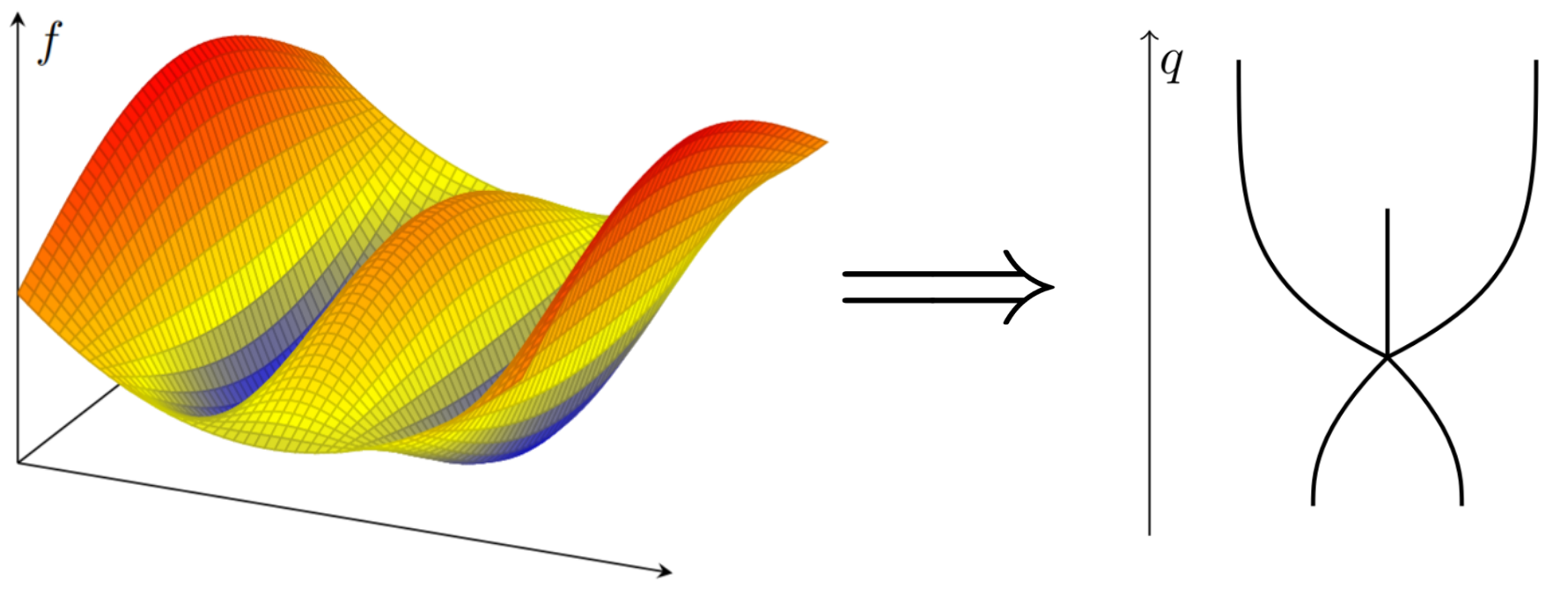
Figure 7: An illustration of a function $f$ on the unit square and its induced Reeb graph. The two local minima of the function produce downward-pointing leaves of equal height on the Reeb graph. Similarly, the three local maxima produce upward-pointing leaves, with the lower maximum producing a lower leaf.

Typically, we picture a Reeb graph $(F,q)$ by thinking of the function $q$ as a “height” function; we imagine that $F$ is situated in space so that $q(x)$ is the altitude of the point $x$. See Figure 7. In the computer science literature, many authors define the Reeb graph by declaring that $x\sim y$ if and only if $x$ and $y$ lie in the same path-connected component instead of the same connected component. While these definitions are not equivalent in general, they are equivalent under reasonable topological assumptions, such as when the level sets of $f$ are locally path-connected.

Reeb graphs are used as summaries of landscapes induced by real functions. While originally designed by Georges Reeb to study functions on smooth manifolds (Reeb, 1946) and independently rediscovered by Kronrod (1950), Reeb graphs were first popularized as a computational tool by Shinagawa et al. (1991). Since then, Reeb graphs have grown in popularity, finding applications in the comparison (Hilaga et al., 2001; Escolano et al., 2013), parameterization (Patanè et al., 2004; Zhang et al., 2005), and denoising (Wood et al., 2004) of shapes, in symmetry detection (Thomas and Natarajan, 2011), and in sketching of static (Chazal and Sun, 2013; Ge et al., 2011) and time-varying (Edelsbrunner et al., 2004) data, among many others. See Biasotti et al. (2008); Yan et al. (2021) for surveys.

Note that not every continuous function $f:X\to{\mathbb{R}}$ will produce the requisite graph structure for the quotient $(X/{\sim},q)$ to be a Reeb graph. For instance, the sine function on $\mathbb{R}$ does not induce a Reeb graph, since the preimage of the interval $(1/3,2/3)$ has infinitely many connected components. Thankfully, many classes of spaces and functions are known to induce Reeb graphs. One list of sufficient conditions is provided by de Silva et al. (2016, Example 2.2).

Figure 8: The Reeb graph of some problem $P$. Based on the downward-pointing leaves of the Reeb graph, this problem’s risk landscape seems to have three basins. The height of the lowest point in the Reeb graph corresponds to the constrained Bayes risk ${\mathcal{B}}(P)$.

Definition 7.6.

Let $P$ be a problem. The Reeb graph of $P$, denoted $\operatorname{Reeb}(P)$, is the Reeb graph induced by the risk function ${\mathcal{R}}_{P}:H\to\mathbb{R}_{\geq 0}$.

The Reeb graph of a problem $P$ is a summary of the risk landscape. (See Figure 8.) For instance, the height of the lowest point of $\operatorname{Reeb}(P)$ is the constrained Bayes risk. If ${\mathcal{R}}_{P}$ has a unique minimizer, then $\operatorname{Reeb}(P)$ will have a unique lowest point. Conversely, if $\operatorname{Reeb}(P)$ has a unique lowest point, then the minimizers of ${\mathcal{R}}_{P}$ form a connected set. Local minima appear as downward-pointing leaves, with the height of the edges corresponding to the depth of the basins around those minima. Similarly, local maxima are represented by upward-pointing leaves. The Reeb graph of $P$ therefore captures information that can be useful for quantifying the complexity of the problem $P$.

Note that for a general problem $P$, one cannot guarantee that ${\mathcal{R}}_{P}$ will induce a graph since the induced quotient of $H$ may not exhibit the necessary graph structure. However, as noted in the discussion after Definition 7.5, conditions that guarantee the necessary graph structure are quite generic. Additionally, our results about Reeb graphs do not actually require the graph structure. Given these facts, we will call the quotient $\operatorname{Reeb}(P)$ a Reeb graph even if it does not exhibit the necessary graph structure.

Reeb graphs can be compared via any of several related metrics. The largest such metric in popular use is called the universal distance (Bauer et al., 2021).

Definition 7.7 (Universal Distance on Reeb graphs).

The universal distance between two Reeb graphs $(F,f)$ and $(G,g)$ is given by

$$d_{\mathrm{U}}((F,f),(G,g)):=\inf_{Z,\widehat{f},\widehat{g}:Z\to\mathbb{R}}\|\widehat{f}-\widehat{g}\|_{\infty}$$

where the infimum ranges over all spaces $Z$ and functions $\widehat{f},\widehat{g}:Z\to{\mathbb{R}}$ such that $\widehat{f}$ induces the Reeb graph $(F,f)$ and $\widehat{g}$ induces the Reeb graph $(G,g)$.

Even with respect to the universal distance, the Reeb graph of a problem is stable under the Connected Risk distance.

Theorem 7.8.

Let $P$ and $P^{\prime}$ be problems. Then

$$|{\mathcal{B}}(P)-{\mathcal{B}}(P^{\prime})|\leq d_{\mathrm{U}}(\operatorname{Reeb}(P),\operatorname{Reeb}(P^{\prime}))\leq d_{\operatorname{RC}}(P,P^{\prime}).$$

Hence the Reeb graph of a problem is a stronger descriptor than the constrained Bayes risk while remaining stable under the Connected Risk distance. The proof can be found in Appendix A.

Example 7.9.

Let $P$ be a problem whose loss $\ell$ is a metric, such as a 0-1 loss in a classification problem, mean absolute error in a regression problem, or a Wasserstein distance in a probability estimation problem. Suppose that we expect noise in the labels of our data such that the average distance under $\ell$ between the true label and the observed label is $\varepsilon_{1}$. Write $\eta^{\prime}$ for the noisy distribution from which the observed data is drawn. Suppose also that the loss function $\ell$ is difficult to exactly compute or has poor optimization properties, but there is an approximation $\ell^{\prime}$ that does not share the same issues and is $\varepsilon_{2}$-close to $\ell$ in the supremum norm. Replacing $\eta$ with the noisy $\eta^{\prime}$ and $\ell$ with the approximation $\ell^{\prime}$ could introduce new local minima to the risk function. We would like to understand how bad these local minima can be. Let $P^{\prime}=(X,Y,\eta^{\prime},\ell,H)$ and $P^{\prime\prime}=(X,Y,\eta^{\prime},\ell^{\prime},H)$. We aim to bound the universal distance between the Reeb graphs of the idealized problem $P$ and the corrupted problem $P^{\prime\prime}$. Since Theorem 4.15 applies to the Connected Risk distance (Remark 7.4), we have

$$d_{\operatorname{RC}}(P,P^{\prime})\leq\varepsilon_{1}.$$

Since $d_{\operatorname{RC}}$ also satisfies Condition 2 from Section 3.3, we also have

$$d_{\operatorname{RC}}(P^{\prime},P^{\prime\prime})\leq\max_{h\in H}\int\big{|}\ell(h(x),y)-\ell^{\prime}(h(x),y)\big{|}\,\eta(dx{\times}dy)\leq\varepsilon_{2}.$$

Then, using the triangle inequality for $d_{\operatorname{RC}}$ and Theorem 7.8, we can write the bound

$$d_{\mathrm{U}}(\operatorname{Reeb}(P),\operatorname{Reeb}(P^{\prime})) \leq d_{\operatorname{RC}}(P,P^{\prime\prime})\leq d_{\operatorname{RC}}(P,P^{\prime})+d_{\operatorname{RC}}(P^{\prime},P^{\prime\prime})\leq\varepsilon_{1}+\varepsilon_{2}.$$

In other words, if we replace the idealized problem $P$ with the corrupted problem $P^{\prime\prime}$, the Reeb graph can change by at most $\varepsilon_{1}+\varepsilon_{2}$ in the universal distance. Hence any downward-pointing leaf of $\operatorname{Reeb}(P)$ of depth more than $2(\varepsilon_{1}+\varepsilon_{2})$ from top to bottom has a corresponding downward-pointing leaf in $\operatorname{Reeb}(P^{\prime\prime})$, and the difference in the heights of the tips of two corresponding leaves is at most $\varepsilon_{1}+\varepsilon_{2}$. We conclude that a basin of depth greater than $2(\varepsilon_{1}+\varepsilon_{2})$ in the risk landscape of the original problem corresponds to some basin in the corrupted problem, and the risk at the bottom of two corresponding basins differ by at most $\varepsilon_{1}+\varepsilon_{2}$. Similarly, any new downward-pointing leaves in the Reeb graph created by corrupting $P$ to get $P^{\prime\prime}$ can be of length at most $2(\varepsilon_{1}+\varepsilon_{2})$ from top to bottom, so any new basins introduced by the corruption can be of depth at most $2(\varepsilon_{1}+\varepsilon_{2})$ from the deepest to highest point of the basin.

8 Discussion

In this work, we argue that, given a notion of distance between supervised learning problems, various corruptions and modifications of problems can be seen from a geometric perspective. We propose the Risk distance and two variants thereof as reasonable choices for this distance notion, bolstering our claims with a garniture of stability results. The development in this paper can be seen as a direct descendent of earlier work in the machine learning community on reductions between learning problems, surrogate losses and different forms of regularisation.

The present work has opened the way for further understanding of machine learning analogous to several productive, related research programs. The idea of the function space lies at the center of the abstract theory of functional analysis (Birkhoff and Kreyszig, 1984, page 259), the development of which which was highly productive for 20th century mathematics (Dieudonné, 1981). Similarly productive for metric geometry was the work of Gromov (1981), which created the metric space of all metric spaces. Other similar examples include category theory, which is concerned with putting relational structures on collection of objects (Mac Lane, 2013), and the theories of optimal transport (Villani, 2008) and information geometry (Amari, 2016), which both propose geometric spaces of probability measures. Common among all of these examples is the viewpoint that to understand an object, it is productive to place it in a larger space of similar objects. Following this viewpoint, the present work opens the door to similar techniques by establishing candidates for spaces of supervised learning problems. In particular, the definition of the Risk distance directly echoes the motifs of an established lineage of distances from metric geometry and optimal transport (Section 2.3). We have shown that the geometry is meaningful; the geometric notion of a geodesic is related to optimal couplings and correspondences (Section 5.1), and that the topological density of classification problems (Section 5.3) is useful in proving the convergence of empirical problems (Section 5.4). We are optimistic that further geometric, topological, and even categorical studies of the space of problems can shed light on questions of interest in supervised learning.

Acknowledgments and Disclosure of Funding

The authors thank Dr. Mark Reid for interesting discussions on topics related to this work that took place during 2010-2011. The authors also thank Dr. Nan Lu for comments on a draft.

F.M. and B.V. were partially supported by the NSF under grants CCF-1740761, DMS-1547357, CCF-2310412 and RI-1901360. R.W. was supported by NICTA and the Deutsche Forschungsgemeinschaft under Germany’s Excellence Strategy — EXC number 2064/1 — Project number 390727645.

Appendix A Relegated Proofs

A.1 Proofs and Details from Section 3

Theorem 3.14.

The only nontrivial pseudometric axiom to prove is the triangle inequality. Furthermore, the claim that $d_{\mathrm{R}}$ vanishes on weakly isomorphic problems will follow from the triangle inequality and the fact that $d_{\mathrm{R}}$ satisfies Condition 1 (Theorem 3.15). That is, if $P^{\prime\prime}$ is common simulation of $P$ and $P^{\prime}$, then $d_{\mathrm{R}}(P,P^{\prime})\leq d_{\mathrm{R}}(P,P^{\prime\prime})+d_{\mathrm{R}}(P^{\prime\prime},P^{\prime})=0+0$. Hence we need only prove that $d_{\mathrm{R}}$ satisfies the triangle inequality.

Let $P_{i}=(X_{i},Y_{i},\eta_{i},\ell_{i},H_{i})$ for $i=1,2,3$. Let $\gamma_{1,2}\in\Pi(\eta_{1},\eta_{2})$, $\gamma_{2,3}\in\Pi(\eta_{2},\eta_{3})$, $R_{1,2}\in{\mathcal{C}}(H_{1},H_{2})$, and $R_{2,3}\in{\mathcal{C}}(H_{2},H_{3})$ be arbitrary. We apply the the gluing lemma (Lemma 2.1) and its counterpart for correspondences (Lemma 2.2). Let $\gamma$ be a gluing of $\gamma_{1,2}$ and $\gamma_{1,3}$, and let $\gamma_{1,3}$ be its marginal on the first and third coordinates. Similarly, let $R$ be a gluing of $R_{1,2}$ and $R_{2,3}$, and let $R_{1,3}$ be its image on its first and third components. We can then write

$$\operatorname{dis}_{P,P^{\prime}}(R_{1,3},\gamma_{1,3})=\sup_{(h_{1},h_{3})\in R_{1,3}} \int\big{|}\ell_{1}(h_{1}(x_{1}),y_{1})-\ell_{3}(h_{3}(x_{3}),y_{3})\big{|}\,\gamma_{1,3}(dx_{1}{\times}dy_{1}{\times}dx_{3}{\times}dy_{3})$$

$$=\sup_{(h_{1},h_{2},h_{3})\in R} \int\big{|}\ell_{1}(h_{1}(x_{1}),y_{1})-\ell_{3}(h_{3}(x_{3}),y_{3})\big{|}\,\gamma(dx_{1}{\times}dy_{1}{\times}dx_{2}{\times}dy_{2}{\times}dx_{3}{\times}dy_{3})$$

$$\leq\sup_{(h_{1},h_{2},h_{3})\in R} \int\big{|}\ell_{1}(h_{1}(x_{1}),y_{1})-\ell_{2}(h_{2}(x_{2}),y_{2})\big{|}\,\gamma(dx_{1}{\times}dy_{1}{\times}dx_{2}{\times}dy_{2}{\times}dx_{3}{\times}dy_{3})$$

$$+\sup_{(h_{1},h_{2},h_{3})\in R} \int\big{|}\ell_{2}(h_{2}(x_{2}),y_{2})-\ell_{3}(h_{3}(x_{3}),y_{3})\big{|}\,\gamma(dx_{1}{\times}dy_{1}{\times}dx_{2}{\times}dy_{2}{\times}dx_{3}{\times}dy_{3})$$

$$=\sup_{(h_{1},h_{2})\in R_{1,2}} \int\big{|}\ell_{1}(h_{1}(x_{1}),y_{1})-\ell_{2}(h_{2}(x_{2}),y_{2})\big{|}\,\gamma_{1,2}(dx_{1}{\times}dy_{1}{\times}dx_{2}{\times}dy_{2})$$

$$+\sup_{(h_{2},h_{3})\in R_{2,3}} \int\big{|}\ell_{2}(h_{2}(x_{2}),y_{2})-\ell_{3}(h_{3}(x_{3}),y_{3})\big{|}\,\gamma_{2,3}(dx_{2}{\times}dy_{2}{\times}dx_{3}{\times}dy_{3})$$

$$\mkern-100.0mu=\operatorname{dis}_{P,P^{\prime}}(R_{1,2},\gamma_{1,2})+\operatorname{dis}_{P,P^{\prime}}(R_{2,3},\gamma_{2,3}).$$

Since we can construct such a $\gamma_{1,3}$ and $R_{1,3}$ from any given $\gamma_{1,2},\gamma_{2,3},R_{1,2},R_{2,3}$, we can take the infimum of each side to get the desired inequality. ∎

Theorem 3.15.

First we demonstrate that the Risk distance does indeed satisfy Conditions 1 and 2. Let $P^{\prime}$ be a simulation of $P$ via the maps $f_{1}:X^{\prime}\to X$ and $f_{2}:Y^{\prime}\to Y$. Define $f:=f_{1}\times f_{2}$. Since $f_{\sharp}\eta^{\prime}=\eta$, $f$ induces a coupling $\gamma_{f}\in\Pi(\eta^{\prime},\eta)$. Define $R\subseteq H^{\prime}\times H$ to be all the pairs $(h^{\prime},h)$ such that $h\circ f_{1}=f_{2}\circ h^{\prime}$. Since $f$ induces a simulation, $R$ is a correspondence. By definition of the Risk distance, we can now write

$$d_{\mathrm{R}}(P,P^{\prime}) \leq\sup_{(h^{\prime},h)\in R}\int\big{|}\ell^{\prime}(h^{\prime}(x^{\prime}),y^{\prime})-\ell(h(x),y)\big{|}\,\gamma_{f}(dx^{\prime}{\times}dy^{\prime}{\times}dx{\times}dy)$$

$$=\sup_{(h^{\prime},h)\in R}\int\big{|}\ell^{\prime}(h^{\prime}(x^{\prime}),y^{\prime})-\ell(h\circ f_{1}(x^{\prime}),f_{2}(y^{\prime}))\big{|}\,\eta^{\prime}(dx^{\prime}{\times}dy^{\prime}).$$

We claim the integrand is identically zero. Indeed,

$$\ell(h\circ f_{1}(x^{\prime}),f_{2}(y^{\prime}))=\ell(f_{2}\circ h^{\prime}(x^{\prime}),f_{2}(y^{\prime}))=\ell^{\prime}(h^{\prime}(x^{\prime}),y^{\prime}).$$

Hence $d_{\mathrm{R}}(P,P^{\prime})=0$.

Let $P=(X,Y,\eta,\ell,H)$ and $P^{\prime}=(X,Y,\eta,\ell^{\prime},H)$ be any pair of problems that differ only in their loss functions. We can bound $d_{\mathrm{R}}(P,P^{\prime})$ by selecting the diagonal coupling between $\eta$ and itself, and the diagonal correspondence between $H$ and itself. This directly yields Condition 2.

Now suppose $d$ is a pseudometric satisfying Conditions 1 and 2, and let $P_{1}$ and $P_{2}$ be problems. Let $\gamma\in\Pi(\eta_{1},\eta_{2})$ and $R\in{\mathcal{C}}(H_{1},H_{2})$ be arbitrary. Define two new problems

$$P^{\prime}_{1} :=(X_{1}\times X_{2},Y_{1}\times Y_{2},\gamma,\ell^{\prime}_{1},R_{\times})$$

$$P^{\prime}_{2} :=(X_{1}\times X_{2},Y_{1}\times Y_{2},\gamma,\ell^{\prime}_{2},R_{\times}),$$

where

• $\ell^{\prime}_{1}((y_{1},y_{2}),(y^{\prime}_{1},y^{\prime}_{2})):=\ell_{1}(y_{1},y^{\prime}_{1})$,

• $\ell^{\prime}_{2}((y_{1},y_{2}),(y^{\prime}_{1},y^{\prime}_{2})):=\ell_{2}(y_{2},y^{\prime}_{2})$,

• $R_{\times}:=\left\{h_{1}\times h_{2}\middle|(h_{1},h_{2})\in R\right\}$.

Then $P^{\prime}_{1}$ is a simulation of $P_{1}$ via the projection maps $X_{1}\times X_{2}\to X_{1}$ and $Y_{1}\times Y_{2}\to Y_{1}$, so by Condition 1, $d(P_{1},P^{\prime}_{1})=0$. Similarly, $d(P_{2},P^{\prime}_{2})=0$. Combining this with Condition 2, we get

$$d(P_{1},P_{2})=d(P^{\prime}_{1},P^{\prime}_{2})$$

$$\leq\max_{h_{1}\times h_{2}\in R_{\times}}\int\big{|}\ell^{\prime}_{1}((h_{1}\times h_{2})(x_{1},x_{2}),(y_{1},y_{2}))-\ell^{\prime}_{2}((h_{1}\times h_{2})(x_{1},x_{2}),(y_{1},y_{2}))\big{|}\,\gamma(dx_{1}{\times}dx_{2}{\times}dy_{1}{\times}dy_{2})$$

$$=\max_{(h_{1},h_{2})\in R}\int\big{|}\ell_{1}(h_{1}(x_{1}),y_{1})-\ell_{2}(h_{2}(x_{2}),y_{2})\big{|}\,\gamma(dx_{1}{\times}dx_{2}{\times}dy_{1}{\times}dy_{2})$$

$$=\operatorname{dis}_{P_{1},P_{2}}(R,\gamma).$$

Taking an infimum over all choices of $\gamma$ and $R$ finishes the proof. ∎

Proposition 3.16.

Let $P$ and $P^{\prime}$ be weakly isomorphic, and let $P^{\prime\prime}$ be a common simulation of both $P$ and $P^{\prime}$ via the maps

$$\leavevmode\hbox to105.66pt{\vbox to49.42pt{\text{[drawing]}}}\qquad\qquad\leavevmode\hbox to102.54pt{\vbox to49.42pt{\text{[drawing]}}}. {X^{\prime\prime}} {X} {X^{\prime}} \scriptstyle{f_{1}} \scriptstyle{g_{1}} {Y^{\prime\prime}} {Y} {Y^{\prime}} \scriptstyle{f_{2}} \scriptstyle{g_{2}} {X^{\prime\prime}} {X} {X^{\prime}} \scriptstyle{f_{1}} \scriptstyle{g_{1}} {Y^{\prime\prime}} {Y} {Y^{\prime}} \scriptstyle{f_{2}} \scriptstyle{g_{2}}$$

There is a unique map $m:X^{\prime\prime}\times Y^{\prime\prime}\to X\times Y\times X^{\prime}\times Y^{\prime}$ making the following diagram commute:

$$\leavevmode\hbox to205.05pt{\vbox to85.62pt{\text{[drawing]}}}. {X^{\prime\prime}\times Y^{\prime\prime}} {X\times Y\times X^{\prime}\times Y^{\prime}} {X\times Y} {X^{\prime}\times Y^{\prime}} \scriptstyle{f_{1}\times f_{2}} \scriptstyle{g_{1}\times g_{2}} \scriptstyle{m} \scriptstyle{\pi_{12}} \scriptstyle{\pi_{34}} {X^{\prime\prime}\times Y^{\prime\prime}} {X\times Y\times X^{\prime}\times Y^{\prime}} {X\times Y} {X^{\prime}\times Y^{\prime}} \scriptstyle{f_{1}\times f_{2}} \scriptstyle{g_{1}\times g_{2}} \scriptstyle{m} \scriptstyle{\pi_{12}} \scriptstyle{\pi_{34}}$$

Define $\gamma:=m_{\sharp}\eta^{\prime\prime}.$ Note that, since the above diagram commutes, $\gamma$ is a coupling between $\eta$ and $\eta^{\prime}$. Also, let $\phi:H^{\prime\prime}\to H$ be such that $\ell^{\prime\prime}_{h^{\prime\prime}}=\ell_{\phi(h^{\prime\prime})}\circ(f_{1}\times f_{2})$ holds $\eta^{\prime\prime}$-almost everywhere. Define $\psi:H^{\prime\prime}\to H^{\prime}$ similarly. Then

$$R:=\left\{(\phi(h^{\prime\prime}),\psi(h^{\prime\prime}))\middle|h^{\prime\prime}\in H^{\prime\prime}\right\}$$

is a correspondence between $H$ and $H^{\prime}$. Finally, compute

$$\operatorname{dis}_{P,P^{\prime}}(R,\gamma) =\sup_{(h,h^{\prime})\in R}\int\big{|}\ell_{h}(x,y)-\ell^{\prime}_{h^{\prime}}(x^{\prime},y^{\prime})\big{|}\,\gamma(dx{\times}dy{\times}dx^{\prime}{\times}dy^{\prime})$$

$$=\sup_{(h,h^{\prime})\in R}\int\big{|}\ell_{h}\circ\pi_{12}(x,y,x^{\prime},y^{\prime})-\ell^{\prime}_{h^{\prime}}\circ\pi_{34}(x,y,x^{\prime},y^{\prime})\big{|}\,\gamma(dx{\times}dy{\times}dx^{\prime}{\times}dy^{\prime})$$

$$=\sup_{(h,h^{\prime})\in R}\int\big{|}\ell_{h}\circ\pi_{12}\circ m(x^{\prime\prime},y^{\prime\prime})-\ell^{\prime}_{h^{\prime}}\circ\pi_{34}\circ m(x^{\prime\prime},y^{\prime\prime})\big{|}\,\eta^{\prime\prime}(dx^{\prime\prime}{\times}dy^{\prime\prime})$$

$$=\sup_{(h,h^{\prime})\in R}\int\big{|}\ell_{h}(f_{1}(x^{\prime\prime}),f_{2}(y^{\prime\prime}))-\ell^{\prime}_{h^{\prime}}(g_{1}(x^{\prime\prime}),g_{2}(y^{\prime\prime}))\big{|}\,\eta^{\prime\prime}(dx^{\prime\prime}{\times}dy^{\prime\prime})$$

$$=\sup_{h^{\prime\prime}\in H^{\prime\prime}}\int\big{|}\ell_{\phi(h^{\prime\prime})}(f_{1}(x^{\prime\prime}),f_{2}(y^{\prime\prime}))-\ell^{\prime}_{\psi(h^{\prime\prime})}(g_{1}(x^{\prime\prime}),g_{2}(y^{\prime\prime}))\big{|}\,\eta^{\prime\prime}(dx^{\prime\prime}{\times}dy^{\prime\prime})$$

$$=\sup_{h^{\prime\prime}\in H^{\prime\prime}}\int\big{|}\ell^{\prime\prime}_{h^{\prime\prime}}(x^{\prime\prime},y^{\prime\prime})-\ell^{\prime\prime}_{h^{\prime\prime}}(x^{\prime\prime},y^{\prime\prime})\big{|}\,\eta^{\prime\prime}(dx^{\prime\prime}{\times}dy^{\prime\prime})=0.$$

Now suppose that there exist $R\in{\mathcal{C}}(H,H^{\prime})$ and $\gamma\in\Pi(\eta,\eta^{\prime})$ such that $\operatorname{dis}_{P,P^{\prime}}(R,\gamma)=0$. Construct a new problem

$$P^{\prime\prime}=(X\times X^{\prime},Y\times Y^{\prime},\tau_{\sharp}\gamma,\ell^{\prime\prime},R_{\times})$$

where

• $\tau:X\times Y\times X^{\prime}\times Y^{\prime}\to X\times X^{\prime}\times Y\times Y^{\prime}$ swaps the second and third components,

• $\ell^{\prime\prime}((y_{1},y^{\prime}_{1}),(y_{2},y^{\prime}_{2})):=\ell(y_{1},y_{2})$

• $R_{\times}:=\left\{h\times h^{\prime}\middle|(h,h^{\prime})\in R\right\}$.

Then the projection maps $f_{1}:X\times X^{\prime}\to X$ and $f_{2}:Y\times Y^{\prime}\to Y$ show that $P^{\prime\prime}$ is a simulation of $P$. Indeed, since $\gamma$ is a coupling of $\eta$ and $\eta^{\prime}$, we have

$$(f_{1}\times f_{2})_{\sharp}\tau_{\sharp}\gamma=((f_{1}\times f_{2})\circ\tau)_{\sharp}\gamma=(\pi_{12})\sharp\gamma=\eta.$$

Furthermore, for any $h\in H$, we can consider some function $(h\times h^{\prime})\in R_{\times}$ and write

$$\ell^{\prime\prime}_{(h\times h^{\prime})}((x,x^{\prime}),(y,y^{\prime})) =\ell^{\prime\prime}((h(x),h^{\prime}(x^{\prime})),(y,y^{\prime}))=\ell(h(x),y)=\ell_{h}(f_{1}(x,x^{\prime}),f_{2}(y,y^{\prime})).$$

Similarly, $P^{\prime\prime}$ is a simulation of $P^{\prime}$ via the projection maps $g_{1}:X\times X^{\prime}\to X^{\prime}$ and $g_{2}:Y\times Y^{\prime}\to Y^{\prime}$. Indeed, an almost identical calculation to the one above shows that $(g_{1}\times g_{2})_{\sharp}\tau_{\sharp}\gamma=\eta^{\prime}$. Furthermore, if $h^{\prime}\in H^{\prime}$ and $(h\times h^{\prime})\in R_{\times}$, we have already calculated that $\ell^{\prime\prime}_{(h\times h^{\prime})}((x,x^{\prime}),(y,y^{\prime}))=\ell(h(x),y)$. The fact that $R$ and $\gamma$ have Risk distortion zero impliex that the latter is equal $\tau_{\sharp}\gamma$-almost everywhere to $\ell^{\prime}(h^{\prime}(x^{\prime}),y^{\prime})=\ell^{\prime}_{h^{\prime}}(g_{1}(x,x^{\prime}),g_{2}(y,y^{\prime}))$, completing the proof. ∎

A.1.1 Connecting the Risk Distance with the Gromov-Wasserstein Distance

Here we discuss a connection with a variant of the Gromov-Wasserstein distance considered by Hang et al. (2019). Given two metric measure spaces $X,X^{\prime}$, a correspondence $R\in{\mathcal{C}}(X,X^{\prime})$ and a coupling $\mu\in\Pi(\mu_{X},\mu_{X^{\prime}})$, one considers the following notion of distortion:

$$\overline{\operatorname{dis}}(R,\mu):=\sup_{(x_{2},x_{2}^{\prime})\in R}\int_{X\times X^{\prime}}\big{|}d_{X}(x_{1},x_{2})-d_{X^{\prime}}(x_{1}^{\prime},x_{2}^{\prime})\big{|}\mu(dx_{1}\times dx_{1}^{\prime}),$$

which leads to the definition

$$\overline{d_{\mathrm{GW}}}(X,X^{\prime}):=\inf_{R,\mu}\overline{\operatorname{dis}}(X,X^{\prime}).$$

This definition, which blends an $L^{\infty}$ matching (expressed through the correspondence $R$) with an $L^{1}$ one (expressed via the coupling $\mu$) was considered by Hang et al. (2019) due its beneficial interaction with stability questions surrounding Fréchet functions in the persistent homology setting.  With the notation and definitions from Section 3.5, we have the following statement.

Proposition A.1.

For all compact metric measure spaces $X$ and $X^{\prime}$: $d_{\mathrm{R}}(i(X),i(X^{\prime}))=\overline{d_{\mathrm{GW}}}(X,X^{\prime}).$

Proof.

First note that any correspondence $R$ between $H_{X}$ and $H_{X^{\prime}}$ can be regarded as a correspondence between $X$ and $X^{\prime}$. This is so because all functions in $H_{X}$ (resp. in $H_{X^{\prime}}$) are constant.

We then have the following calculation:

$$\operatorname{dis}_{i(X),i(X^{\prime})}(R,\gamma) =\sup_{(h,h^{\prime})\in R}\int\big{|}d_{X}(h(x_{0}),x_{1})-d_{X^{\prime}}(h^{\prime}(x^{\prime}_{0}),x^{\prime}_{1})\big{|}\,\gamma(dx_{0}{\times}dx_{1}{\times}dx^{\prime}_{0}{\times}dx^{\prime}_{1})$$

$$=\sup_{(x_{2},x^{\prime}_{2})\in R}\int\big{|}d_{X}(x_{2},x_{1})-d_{X^{\prime}}(x^{\prime}_{2},x^{\prime}_{1})\big{|}\,\gamma(dx_{0}{\times}dx_{1}{\times}dx^{\prime}_{0}{\times}dx^{\prime}_{1})$$

$$=\sup_{(x_{2},x^{\prime}_{2})\in R}\int\big{|}d_{X}(x_{2},x_{1})-d_{X^{\prime}}(x^{\prime}_{2},x^{\prime}_{1})\big{|}\,(\pi_{2,4})_{\sharp}\gamma(dx_{0}{\times}dx_{1}{\times}dx^{\prime}_{0}{\times}dx^{\prime}_{1})$$

$$=\overline{\operatorname{dis}}(R,(\pi_{2,4})_{\sharp}\gamma).$$

The above equality immediately implies that $d_{\mathrm{R}}(i(X),i(X^{\prime}))\geq\overline{d_{\mathrm{GW}}}(X,X^{\prime}).$ The reverse inequality can be obtained from the following fact. Let $\tau:X\times X^{\prime}\to X\times X\times X^{\prime}\times X^{\prime}$ be the map $(x,x^{\prime})\mapsto(x,x,x^{\prime},x^{\prime})$. Then, if $\mu\in\Pi(\mu_{X},\mu_{X^{\prime}})$, $\gamma_{\mu}:=\tau_{\sharp}\mu$ is an element of $\Pi((\Delta_{X})_{\sharp}\mu_{X},(\Delta_{X^{\prime}})_{\sharp}\mu_{X^{\prime}})$. Since $\pi_{2,4}\circ\tau=\mathrm{id}:X\times X^{\prime}\to X\times X^{\prime}$, the identity map, $(\pi_{2,4})_{\sharp}\gamma_{\mu}=\mu$ and the calculation above gives $\operatorname{dis}_{i(X),i(X^{\prime})}(R,\gamma_{\mu})=\overline{\operatorname{dis}}(\mu)$. From this we obtain that $d_{\mathrm{R}}(i(X),i(X^{\prime}))\leq\overline{d_{\mathrm{GW}}}(X,X^{\prime}).$ ∎

Proposition 3.20.

If $d_{\mathrm{GW},p}(X,X^{\prime})=0$, then $X$ and $X^{\prime}$ are isomorphic as metric measure spaces. Using the isomorphism $X\to X^{\prime}$, it is not hard to construct a coupling and correspondence between $i(X)$ and $i(X^{\prime})$ of risk distortion zero. Conversely, let $d_{\mathrm{R}}(i(X),i(X^{\prime}))=0$. It is not a priori obvious that there exists a correspondence $R\in{\mathcal{C}}(H_{X},H_{X^{\prime}})$ and a coupling $\gamma\in\Pi((\Delta_{X})_{\sharp}\mu_{X},(\Delta_{X^{\prime}})_{\sharp}\mu_{X^{\prime}})$ that together achieve the infimal risk distortion of zero. In Section 5.2, we will explore the existence of such couplings and correspondences. In this case, since $d_{X}$ and $d_{X^{\prime}}$ are continuous functions and $X$ and $X^{\prime}$ are assumed to be compact, Theorem 5.6 does guarantee that there exists an $R$ and a $\gamma$ with $\operatorname{dis}_{i(X),i(X^{\prime})}(R,\gamma)=0$. Furthermore, recall that a correspondence $R$ between $H_{X}$ and $H_{X^{\prime}}$ is equivalent to a correspondence between $X$ and $X^{\prime}$. Hence, as in the proof of Proposition A.1, we have $0=\operatorname{dis}_{i(X),i(X^{\prime})}(R,\gamma)=\overline{\operatorname{dis}}(R,(\pi_{2,4})_{\sharp}\gamma)$. Set $R^{\prime}:=\operatorname{supp}((\pi_{2,4})_{\sharp}\gamma)$. Since the integrand defining $\overline{\operatorname{dis}}(R,(\pi_{2,4})_{\sharp}\gamma)$ is continuous and non-negative, we can conclude that

$$d_{X}(x_{2},x_{1})=d_{X^{\prime}}(x^{\prime}_{2},x^{\prime}_{1})$$

for all $(x_{2},x^{\prime}_{2})\in R$ and $(x_{1},x^{\prime}_{1})\in R^{\prime}$. Furthermore, since $(\pi_{2,4})_{\sharp}\gamma$ is a coupling between the fully supported measures $\mu_{X}$ and $\mu_{X^{\prime}}$, its support $R^{\prime}$ is a correspondence between $X$ and $X^{\prime}$ (see Mémoli, 2011, Lemma 2.2).  We claim that $R=R^{\prime}$. Indeed, if $(x_{2},x^{\prime}_{2})\in R$, selecting any pair $(x_{2},x^{\prime}_{1})\in R^{\prime}$ yields $d_{X}(x_{2},x_{2})=d_{X^{\prime}}(x^{\prime}_{2},x^{\prime}_{1})$ and hence $x^{\prime}_{2}=x^{\prime}_{1}$. This shows $R\subseteq R^{\prime}$, and a similar argument shows the opposite inclusion. We furthermore claim that $R$ is the graph of a bijection. Let $(x,x^{\prime}),(x,x^{\prime\prime})\in R$. Then $d_{X}(x,x)=d_{X^{\prime}}(x^{\prime},x^{\prime\prime})$, showing $x^{\prime}=x^{\prime\prime}$. Again, a similar argument holds when reversing the roles of $X$ and $X^{\prime}$.  Let $f:X\to X^{\prime}$ be the bijection whose graph is $R$. Then equation (A.1.1) becomes $d_{X}(x_{2},x_{1})=d_{X^{\prime}}(f(x_{2}),f(x_{1}))$, showing that $f$ is an isometry. Additionally, since $(\pi_{2,4})_{\sharp}\gamma$ is a coupling of $\mu_{X}$ and $\mu_{X^{\prime}}$ which is supported on $R$, the projections $R\to X$ and $R\to X^{\prime}$ are measure-preserving bijections. It follows that the composition of the natural maps $X\to R\to X^{\prime}$, which agrees with $f$, is a measure-preserving map. Hence $f$ is an isomorphism of metric measure spaces, and $d_{\mathrm{GW},1}(X,X^{\prime})=0$. ∎

A.2 Proofs from Section 4

Theorem 4.3.

Let $\operatorname{Prob}_{1}({\mathbb{R}}_{\geq 0})\subseteq\operatorname{Prob}({\mathbb{R}}_{\geq 0})$ be the subset of probability measures with finite mean. The $\mathrm{mean}$ function

$$\mathrm{mean}:\operatorname{Prob}_{1}({\mathbb{R}}_{\geq 0}) \to{\mathbb{R}}_{\geq 0}$$

is 1-Lipschitz when the domain is endowed with the 1-Wasserstein distance $d_{\mathrm{W},1}$ and the codomain is given the Euclidean distance. We will now “lift” the $\mathrm{mean}$ function to a function on power sets by applying it elementwise. That is, we define

$$\mathrm{Pow}(\mathrm{mean}):\mathrm{Pow}(\operatorname{Prob}_{1}({\mathbb{R}}_{\geq 0})) \to\mathrm{Pow}({\mathbb{R}}_{\geq 0})$$

$$\left\{\alpha_{i}\middle|i\in I\right\} \mapsto\left\{\mathrm{mean}(\alpha_{i})\middle|i\in I\right\}.$$

We also endow the domain and codomain with the Hausdorff distance, where the underlying metrics are $d_{\mathrm{W},1}$ and the Euclidean distance respectively. Since the $\mathrm{mean}$ function is 1-Lipschitz, so is $\mathrm{Pow}(\mathrm{mean})$. The infimum function $\inf:\mathrm{Pow}(\mathbb{R}_{\geq 0})\to\mathbb{R}_{\geq 0}$ 1-Lipschitz as well, so the composition $\inf\circ\mathrm{Pow}(\mathrm{mean})$ is 1-Lipschitz. In other words, for any $M,N\subseteq\operatorname{Prob}_{1}({\mathbb{R}}_{\geq 0})$, we have

$$\big{|}\inf\left\{\mathrm{mean}(\mu)\middle|\mu\in M\right\}-\inf\left\{\mathrm{mean}(\nu)\middle|\nu\in N\right\}\big{|}\leq d_{\mathrm{H}}^{d_{\mathrm{W},1}}(M,N).$$

By Proposition 4.2, applying this inequality when $M$ and $N$ are loss profile sets gives the first desired inequality.

To prove the second inequality, observe that $d(P,P^{\prime}):=d_{\mathrm{H}}^{d_{\mathrm{W},1}}(L(P),L(P^{\prime}))$ is a pseudometric on the collection of all problems. By Theorem 3.15, we need only show that $d$ satisfies Conditions 1 and 2. Beginning with Condition 1, let $P^{\prime}$ be a simulation of $P$ via the maps $f_{1}:X^{\prime}\to X$ and $f_{2}:Y^{\prime}\to Y$. Let $f:=f_{1}\times f_{2}$. If $h\in H$ and $h^{\prime}\in H^{\prime}$ are such that $f_{2}\circ h=h^{\prime}\circ f_{2}$, then

$$\ell^{\prime}_{h^{\prime}}\circ f(x,y) =\ell^{\prime}(h^{\prime}\circ f_{1}(x),f_{2}(y))=\ell^{\prime}(f_{2}\circ h(x),f_{2}(y))=\ell(h(x),y)=\ell_{h}(x,y).$$

Hence the loss profiles of $h$ and $h^{\prime}$ are equal:

$$(\ell^{\prime}_{h^{\prime}})_{\sharp}\eta^{\prime} =(\ell^{\prime}_{h^{\prime}}\circ f)_{\sharp}\eta=(\ell_{h})_{\sharp}\eta.$$

Such an $h^{\prime}\in H^{\prime}$ exists for every $h\in H$ and vice versa by definition of a simulation, so we conclude that $L(P)=L(P^{\prime})$ and $d(P,P^{\prime})=0$.

For Condition 2, let $h\in H$. We can bound the Wasserstein distance between the loss profiles $(\ell_{h})_{\sharp}\eta$ and $(\ell^{\prime}_{h})_{\sharp}\eta$ by selecting the coupling $(\ell_{h},\ell^{\prime}_{h})_{\sharp}\eta$, which yields

$$d_{\mathrm{W},1}((\ell_{h})_{\sharp}\eta,(\ell^{\prime}_{h})_{\sharp}\eta) \leq\int\big{|}r-s\big{|}(\ell_{h},\ell^{\prime}_{h})_{\sharp}\eta(dr{\times}ds)$$

$$=\int\big{|}\ell_{h}(x,y)-\ell^{\prime}_{h}(x,y)\big{|}\,\eta(dx\times dy).$$

Since this holds for all $h$, Condition 2 is satisfied as well. ∎

Theorem 4.7.

Let $R\in{\mathcal{C}}(H,H^{\prime})$ and $\gamma\in\Pi(\eta,\eta^{\prime})$ be arbitrary. Then

$$\big{|}R_{m}(P)-R_{m}(P^{\prime})\big{|}$$

$$= \bigg{|}\int\int\sup_{h\in H}\frac{1}{m}\sum_{i=1}^{m}\sigma_{i}\ell_{h}(x_{i},y_{i})\,\mathrm{Rad}^{\otimes m}(d\sigma)\,\eta^{\otimes m}(d\overline{x}\times d\overline{y})$$

$$- \int\int\sup_{h^{\prime}\in H^{\prime}}\frac{1}{m}\sum_{i=1}^{m}\sigma_{i}\ell^{\prime}_{h^{\prime}}(x^{\prime}_{i},y^{\prime}_{i})\,\mathrm{Rad}^{\otimes m}(d\sigma)\,\eta^{\otimes m}(d\overline{x}\times d\overline{y})\bigg{|}$$

$$\leq \int\int\sup_{(h,h^{\prime})\in R}\left|\frac{1}{m}\sum_{i=1}^{m}\sigma_{i}\ell_{h}(x_{i},y_{i})-\frac{1}{m}\sum_{i=1}^{m}\sigma_{i}\ell_{h}(x^{\prime}_{i},y^{\prime}_{i})\right|\,\mathrm{Rad}^{\otimes m}(d\sigma)\,\gamma^{\otimes m}(d\overline{x}{\times}d\overline{y}{\times}d\overline{x}^{\prime}{\times}d\overline{y}^{\prime})$$

$$\leq \int\sup_{(h,h^{\prime})\in R}\frac{1}{m}\sum_{i=1}^{m}\big{|}\ell_{h}(x_{i},y_{i})-\ell_{h}(x^{\prime}_{i},y^{\prime}_{i})\big{|}\,\gamma^{\otimes m}(d\overline{x}{\times}d\overline{y}{\times}d\overline{x}^{\prime}{\times}d\overline{y}^{\prime}).$$

Let $\widehat{\gamma}$ be the unique probability measure on the countable product $(X\times Y)^{\mathbb{N}}$ whose marginal on the first $m$ components is $\gamma^{\otimes m}$. Then the above integral can be written

$$\int\sup_{(h,h^{\prime})\in R}\frac{1}{m}\sum_{i=1}^{m}\big{|}\ell_{h}(x_{i},y_{i})-\ell_{h}(x^{\prime}_{i},y^{\prime}_{i})\big{|}\,\widehat{\gamma}(d\overline{x}{\times}d\overline{y}{\times}d\overline{x}^{\prime}{\times}d\overline{y}^{\prime}).$$

Now we let $m\to\infty$. By the Glivenko-Cantelli assumption, the integrand of (A.2) converges almost everywhere to

$$\sup_{(h,h^{\prime})\in R}\int\big{|}\ell_{h}(x,y)-\ell^{\prime}_{h^{\prime}}(x^{\prime},y^{\prime})\big{|}\,\gamma(dx{\times}dy{\times}dx^{\prime}{\times}dy^{\prime})=\operatorname{dis}_{P,P^{\prime}}(R,\gamma).$$

Furthermore, since $\ell$ and $\ell^{\prime}$ are bounded, by the dominated convergence theorem, the limit of (A.2) itself is $\operatorname{dis}_{P,P^{\prime}}(R,\gamma)$ as well. Infimizing over the choices of $R$ and $\gamma$ completes the proof. ∎

Lemma 4.14.

We aim to bound $d_{\mathrm{R}}(P,P^{\prime})$. To this end, define

$$\Delta:X\times Y\times Y \to X\times Y\times X\times Y$$

$$(x,y,y^{\prime}) \mapsto(x,y,x,y^{\prime}).$$

Let $\Pi_{g}$ be the collection of all gluings of $\eta$ and $\eta^{\prime}$ along $X$. That is,

$$\Pi_{g}:=\left\{\lambda\in\operatorname{Prob}(X\times Y\times Y)\middle|(\pi_{1,2})_{\sharp}\lambda=\eta,(\pi_{1,3})_{\sharp}\lambda=\eta^{\prime}\right\}.$$

By the gluing lemma (Lemma 2.1), $\Pi_{g}$ is nonempty. Note that if $\lambda\in\Pi_{g}$, then $\Delta_{\sharp}\lambda\in\Pi(\eta,\eta^{\prime})$.

We can then write

$$d_{\mathrm{R}}(P,P^{\prime}) \leq\inf_{\gamma\in\Pi(\eta,\eta^{\prime})}\int\big{|}\ell(h(x),y)-\ell(h(x^{\prime}),y^{\prime})\big{|}\,\gamma(dx\times dy\times dx^{\prime}\times dy^{\prime})$$

$$\leq\inf_{\lambda\in\Pi_{g}}\int\big{|}\ell(h(x),y)-\ell(h(x^{\prime}),y^{\prime})\big{|}\,\Delta_{\sharp}\lambda(dx\times dy\times dx^{\prime}\times dy^{\prime})$$

$$=\inf_{\lambda\in\Pi_{g}}\int\big{|}\ell(h(x),y)-\ell(h(x),y^{\prime})\big{|}\,\lambda(dx\times dy\times dy^{\prime})$$

$$\leq C\inf_{\lambda\in\Pi_{g}}\int d_{Y}(y,y^{\prime})\,\lambda(dx\times dy\times dy^{\prime}).$$

Now suppose $\tau\in\Pi(\beta,\beta^{\prime})$. Then one can show that the induced coupling $\lambda\in\operatorname{Prob}(X\times Y\times Y)$, which has $X$-marginal $\alpha$ and $X$-disintegration $\tau:X\to\operatorname{Prob}(Y\times Y^{\prime})$, lies in $\Pi_{g}$. Hence we can continue our string of inequalities with

$$\leq C\inf_{\tau\in\Pi(\beta,\beta^{\prime})}\int\int d_{Y}(y,y^{\prime})\,\tau(x)(dy\times dy^{\prime})\alpha(dx) =Cd_{\mathrm{W},1}^{d_{Y}}(\beta,\beta^{\prime}),$$

the desired bound. ∎

Theorem 4.15.

By Lemma 4.14, we obtain

$$d_{\mathrm{R}}(P,P^{\prime})\leq Cd_{\mathrm{W},1}^{d_{Y}}(\beta,\beta^{\prime}).$$

We can write $\beta$ and $\beta^{\prime}$ as

$$\beta =\Delta_{X}\cdot(\delta_{\operatorname{Id}_{X}}\otimes\beta)\cdot\delta_{\pi_{2}}$$

$$\beta^{\prime} =\Delta_{X}\cdot(\delta_{\operatorname{Id}_{X}}\otimes\beta)\cdot N.$$

Here $\Delta_{X}$ is the diagonal kernel $\Delta_{X}:X\to X\times X$ given by $\Delta_{X}(x)=\delta_{(x,x)}$, and $\otimes$ represents the product of Markov kernels. Note that

$$\alpha\cdot\Delta_{X}\cdot(\delta_{\operatorname{Id}_{X}}\otimes\beta)=\eta.$$

Hence $\Delta_{X}\cdot(\delta_{\operatorname{Id}_{X}}\otimes\beta)$ is an example of a measure non-increasing Markov kernel (Patterson, 2020, Proposition 6.1), so we can write

$$d_{\mathrm{W},1}^{d_{Y}}(\Delta_{X}\cdot(\delta_{\operatorname{Id}_{X}}\otimes\beta)\cdot\delta_{\pi_{2}},\,\Delta_{X}\cdot(\delta_{\operatorname{Id}_{X}}\otimes\beta)\cdot N)\leq d_{\mathrm{W},1}^{d_{Y}}(\delta_{\pi_{2}},N),$$

completing the proof. ∎

A.3 Proofs from Section 5

Lemma 5.4.

The following proof uses ideas similar to those in the proof of Theorem 4.1 of Villani (2008), with the additional wrinkle of an integrand that depends on $n$ and an additional trick of “hot-swapping” an integrand with a lower semi-continuous version.

Since the topology on the domain is induced by a pseudometric, it is enough to consider an arbitrary convergent sequence $(h_{n},h^{\prime}_{n},\gamma_{n})\to(h,h^{\prime},\gamma)$ in $H\times H^{\prime}\times\Pi(\eta,\eta^{\prime})$ and check that,

$$\widetilde{\operatorname{dis}}_{P,P^{\prime}}(h,h^{\prime},\gamma)\leq\liminf_{n}\widetilde{\operatorname{dis}}_{P,P^{\prime}}(h_{n},h^{\prime}_{n},\gamma_{n}).$$

To that end, let $\varepsilon>0$ be arbitrary. We define a function

$$f:X\times Y\times X^{\prime}\times Y^{\prime} \to{\mathbb{R}}_{\geq 0}$$

$$(x_{0},y_{0},x^{\prime}_{0},y^{\prime}_{0}) \mapsto\liminf_{(x,y,x^{\prime},y^{\prime})\to(x_{0},y_{0},x^{\prime}_{0},y^{\prime}_{0})}|\ell_{h}(x,y)-\ell^{\prime}_{h^{\prime}}(x^{\prime},y^{\prime})|.$$

That is, $f$ is a lower semi-continuous version of the function $|\ell_{h}-\ell^{\prime}_{h^{\prime}}|$, constructed by modifying the latter on its points of discontinuity. Indeed, $f$ and $|\ell_{h}-\ell^{\prime}_{h^{\prime}}|$ agree wherever the latter is continuous, which is $\gamma$-almost everywhere on $X\times Y\times X^{\prime}\times Y^{\prime}$. To wit, if $A\subseteq X\times Y$ and $A^{\prime}\subseteq X^{\prime}\times Y^{\prime}$ are the points at which $\ell_{h}$ and $\ell^{\prime}_{h^{\prime}}$ are discontinuous respectively, then the points of discontinuity for $|\ell_{h}-\ell^{\prime}_{h^{\prime}}|$ lie within $A\times X^{\prime}\times Y^{\prime}\cup X\times Y\times A^{\prime}$, and one can check

$$\gamma(A\times X^{\prime}\times Y^{\prime}\cup X\times Y\times A^{\prime})\leq\gamma(A\times X^{\prime}\times Y^{\prime})+\gamma(X\times Y\times A^{\prime})=\eta(A)+\eta^{\prime}(A^{\prime})=0.$$

Hence $f$ is a lower semi-continuous function which agrees $\gamma$-almost everywhere with $|\ell_{h}-\ell^{\prime}_{h^{\prime}}|$.

We can now proceed with our convergence argument; let $\varepsilon>0$ and pick $N$ large enough that, for all $n\geq N$,

• $d_{\ell,\eta}(h_{n},h)<\varepsilon/3$,

• $d_{\ell^{\prime},\eta^{\prime}}(h^{\prime}_{n},h^{\prime})<\varepsilon/3$,

• and

  $$\int f(x,y,x^{\prime},y^{\prime})\,d\gamma<\int f(x,y,x^{\prime},y^{\prime})\,d\gamma_{n}+\varepsilon/3.$$

The latter is possible since $f$ is a lower semi-continuous, non-negative function (Villani, 2008, Lemma 4.3). Then for large $n$ we have

$$\widetilde{\operatorname{dis}}_{P,P^{\prime}}(h,h^{\prime},\gamma) =\int\big{|}\ell_{h}(x,y)-\ell^{\prime}_{h^{\prime}}(x^{\prime},y^{\prime})\big{|}\,d\gamma$$

$$=\int f(x,y,x^{\prime},y^{\prime})\,d\gamma$$

$$\leq\int f(x,y,x^{\prime},y^{\prime})\,d\gamma_{n}+\varepsilon/3$$

$$=\int\big{|}\ell_{h}(x,y)-\ell^{\prime}_{h^{\prime}}(x^{\prime},y^{\prime})\big{|}\,d\gamma_{n}+\varepsilon/3$$

$$\leq\int\big{|}\ell_{h}(x,y)-\ell_{h_{n}}(x,y)\big{|}\,d\gamma_{n}$$

$$+\int\big{|}\ell_{h_{n}}(x,y)-\ell^{\prime}_{h^{\prime}_{n}}(x^{\prime},y^{\prime})\big{|}\,d\gamma_{n}$$

$$+\int\big{|}\ell_{h^{\prime}_{n}}(x^{\prime},y^{\prime})-\ell^{\prime}_{h^{\prime}}(x^{\prime},y^{\prime})\big{|}\,d\gamma_{n}+\varepsilon/3$$

$$=d_{\ell,\eta}(h,h_{n})+\widetilde{\operatorname{dis}}_{P,P^{\prime}}(h_{n},h^{\prime}_{n},\gamma_{n})+d_{\ell^{\prime},\eta^{\prime}}(h^{\prime},h^{\prime}_{n})+\varepsilon/3<\widetilde{\operatorname{dis}}_{P,P^{\prime}}(h_{n},h^{\prime}_{n},\gamma_{n})+\varepsilon$$

as desired. In the last equality, we replace $\gamma_{n}$ with $\eta$ and $\eta^{\prime}$ in the first and last integrals respectively since $\gamma_{n}$ is a coupling between $\eta$ and $\eta^{\prime}$. ∎

In order to prove Lemma 5.5 we will require the following technical lemma.

Lemma A.2.

Let $X$ be a pseudometric space and $f:X\to{\mathbb{R}}$ a lower semi-continuous function. Then the map

$$F:\mathrm{Pow}(X) \to{\mathbb{R}}$$

$$A \mapsto\sup_{a\in A}f(a)$$

is lower semi-continuous as well when the power set $\mathrm{Pow}(X)$ is endowed with the Hausdorff metric.

Proof.

Let the sequence of subsets $A_{n}\subseteq X$ converge to $A\subseteq X$ in the Hausdorff distance. Select $a^{\prime}\in A$ such that

$$\sup_{a\in A}f(a)<f(a^{\prime})+\varepsilon/2.$$

Select also a sequence $a^{\prime}_{n}\in X$ such that $a^{\prime}_{n}\in A_{n}$ for all $n$, and $a^{\prime}_{n}$ converges to $a^{\prime}$. Then for sufficiently large $n$,

$$f(a^{\prime})<f(a^{\prime}_{n})+\varepsilon/2$$

by lower semi-continuity of $f$. Hence for large $n$,

$$F(A)=\sup_{a\in A}f(a)<f(a^{\prime})+\varepsilon/2<f(a^{\prime}_{n})+\varepsilon\leq\sup_{a\in A_{n}}f(a)+\varepsilon=F(A_{n})+\varepsilon.$$

Hence $F$ is lower semi-continuous. ∎

Lemma 5.5.

Write

$$\operatorname{dis}_{P,P^{\prime}}(R,\gamma)=\sup_{((h,\nu),(h^{\prime},\nu^{\prime}))\in R\times\{\gamma\}}\widetilde{\operatorname{dis}}_{P,P^{\prime}}(h,h^{\prime},\nu).$$

Using the above equation, we can think of $\operatorname{dis}_{P,P^{\prime}}$ as a composition of two maps:

$${\mathcal{C}}(H,H^{\prime})\times\Pi(\eta,\eta^{\prime}) \to\mathrm{Pow}(H\times H^{\prime}\times\Pi(\eta,\eta^{\prime}))$$

$$(R,\gamma) \mapsto R\times\{\gamma\},$$

and

$$\mathrm{Pow}(H\times H^{\prime}\times\Pi(\eta,\eta^{\prime})) \to{\mathbb{R}}$$

$$A \mapsto\sup_{(h,h^{\prime},\nu)\in A}\widetilde{\operatorname{dis}}_{P,P^{\prime}}(h,h^{\prime},\nu).$$

The second map is lower semi-continuous by Lemma A.2. The first map is an isometric embedding. Indeed, let $d_{w}$ be a metric on $\Pi(\eta,\eta^{\prime})$ that induces the weak topology. The topology on the domain ${\mathcal{C}}(H,H^{\prime})\times\Pi(\eta,\eta^{\prime})$ is induced by the metric

$$d_{1}((R_{1},\gamma_{1}),(R_{2},\gamma_{2})):=\max\{d_{\mathrm{H}}(R_{1},R_{2}),d_{w}(\gamma_{1},\gamma_{2})\}.$$

Meanwhile, unwrapping the metric on the codomain $\mathrm{Pow}(H\times H^{\prime}\times\Pi(\eta,\eta^{\prime}))$ gives us

$$d_{2}(R_{1}\times\{\gamma_{1}\},R_{2}\times\{\gamma_{2}\})$$

$$:=\max\Bigg{\{} \sup_{(h_{1},h_{1}^{\prime},\nu_{1})\in R_{1}\times\{\gamma_{1}\}}\inf_{(h_{2},h_{2}^{\prime},\nu_{2})\in R_{2}\times\{\gamma_{2}\}}\max\{d_{H\times H^{\prime}}((h_{1},h_{1}^{\prime})(h_{2},h_{2}^{\prime})),d_{w}(\nu_{1},\nu_{2})\},$$

$$\sup_{(h_{2},h_{2}^{\prime},\nu_{2})\in R_{2}\times\{\gamma_{2}\}}\inf_{(h_{1},h_{1}^{\prime},\nu_{1})\in R_{1}\times\{\gamma_{1}\}}\max\{d_{H\times H^{\prime}}((h_{1},h_{1}^{\prime})(h_{2},h_{2}^{\prime})),d_{w}(\nu_{1},\nu_{2})\}\Bigg{\}}$$

$$=\max\Bigg{\{} \sup_{(h_{1},h_{1}^{\prime})\in R_{1}}\inf_{(h_{2},h_{2}^{\prime})\in R_{2}}d_{H\times H^{\prime}}((h_{1},h_{1}^{\prime})(h_{2},h_{2}^{\prime})),$$

$$\sup_{(h_{2},h_{2}^{\prime})\in R_{2}}\inf_{(h_{1},h_{1}^{\prime})\in R_{1}}d_{H\times H^{\prime}}((h_{1},h_{1}^{\prime})(h_{2},h_{2}^{\prime})),d_{w}(\gamma_{1},\gamma_{2})\Bigg{\}}$$

$$=\max\{ d_{\mathrm{H}}(R_{1},R_{2}),d_{w}(\gamma_{1},\gamma_{2})\},$$

which is the definition of $d_{1}((R_{1},\gamma_{1}),(R_{2},\gamma_{2}))$. Hence the composition is lower semi-continuous. ∎

Theorem 5.6.

Throughout this proof, let ${\mathcal{C}}_{c}(H,H^{\prime})\subseteq{\mathcal{C}}(H,H^{\prime})$ be the collection of topologically closed correspondences between $H$ and $H^{\prime}$.

Note that $\Pi(\eta,\eta^{\prime})$ is compact under the weak topology, since $\eta$ and $\eta^{\prime}$ are probability measures on Polish spaces. Compactness of such coupling spaces is proved, for instance, by Sturm (2012, Lemma 1.2), Chowdhury and Mémoli (2019, Lemma 2.2) and in a proof by Villani (2003, Prop 2.1). Similarly, ${\mathcal{C}}_{c}(H,H^{\prime})$ is compact under the Hausdorff distance when $H$ and $H^{\prime}$ are compact. (Here we are equipping $H$ and $H^{\prime}$ with the pseudometrics $d_{\ell,\eta}$ and $d_{\ell^{\prime},\eta^{\prime}}$ respectively, introduced in Section 4.5.) As noted by Chowdhury and Mémoli (2018, Section 2), compactness of such correspondence spaces follows from a theorem of Blaschke (Burago et al., 2001, Theorem 7.3.8). Indeed, Blaschke’s theorem implies that the space of all closed subsets of $H\times H^{\prime}$ is compact. Since ${\mathcal{C}}_{c}(H,H^{\prime})$ is closed in the set of all closed subsets of $H\times H^{\prime}$, being the intersection of the preimages of $H$ and $H^{\prime}$ under the projection maps onto the first and second coordinates respectively, we get that ${\mathcal{C}}_{c}(H,H^{\prime})$ is compact as well.

The lower semi-continuity of $\operatorname{dis}_{P,P^{\prime}}$ (Lemma 5.5) in particular implies that for any correspondence $R$ and coupling $\gamma$, $\operatorname{dis}(R,\gamma)=\operatorname{dis}(\mathrm{cl}(R),\gamma)$, where $\mathrm{cl}$ represents topological closure. Indeed, since $R$ and its closure are distance zero apart in the Hausdorff distance, the constant sequence $R$ converges to $\mathrm{cl}(R)$ and vice versa. Hence, when computing the Risk distance, we can restrict our attention to closed correspondences:

$$d_{\mathrm{R}}(P,P^{\prime})=\inf_{\begin{subarray}{c}R\in{\mathcal{C}}(H,H^{\prime})\\ \gamma\in\Pi(\eta,\eta^{\prime})\end{subarray}}\operatorname{dis}_{P,P^{\prime}}(R,\gamma)=\inf_{\begin{subarray}{c}R\in{\mathcal{C}}_{c}(H,H^{\prime})\\ \gamma\in\Pi(\eta,\eta^{\prime})\end{subarray}}\operatorname{dis}_{P,P^{\prime}}(R,\gamma).$$

Since $\operatorname{dis}_{P,P^{\prime}}$ is lower semi-continuous, and the latter infimum is over a pair of compact sets, the infimum must be achieved. ∎

Theorem 5.11.

First consider an arbitrary finite partition $Q$ of $Y$. Let $\pi:Y\to Q$ be the quotient map. Since $(\operatorname{Id}_{X}\times\pi)_{\sharp}\eta=\eta_{Q}$, the map $\operatorname{Id}_{X}\times\pi$ induces a coupling $\gamma_{(\operatorname{Id}_{X}\times\pi)}$ between $\eta$ and $\eta_{Q}$. We also define a correspondence $R_{\pi}$ between $H$ and $H_{Q}$ by pairing each $h\in H$ with $\pi\circ h\in H_{Q}$. Selecting this coupling and correspondence gives us a bound on the Risk distance:

$$d_{\mathrm{R}}(P,P_{Q}) \leq\operatorname{dis}_{P,P_{Q}}(R_{\pi},\gamma_{\operatorname{Id}_{X}\times\pi})$$

$$\leq\sup_{(h,\pi\circ h)\in R_{\pi}}\int\big{|}\ell(h(x),y)-\ell^{\prime}(\pi\circ h(x^{\prime}),y^{\prime})\big{|}\,\gamma_{(\operatorname{Id}_{X}\times\pi)}(dx\times dy\times dx^{\prime}\times dy^{\prime})$$

$$=\sup_{h\in H}\int\big{|}\ell(h(x),y)-\ell^{\prime}(\pi\circ h(x),\pi(y))\big{|}\,\eta(dx\times dy)$$

$$=\sup_{h\in H}\int\sup_{\begin{subarray}{c}y^{\prime}\in\pi\circ h(x)\\ y^{\prime\prime}\in\pi(y)\end{subarray}}\ell(y^{\prime},y^{\prime\prime})-\ell(h(x),y)\,\eta(dx\times dy)$$

$$\leq\sup_{h\in H}\int\sup_{\begin{subarray}{c}y^{\prime}\in\pi\circ h(x)\\ y^{\prime\prime}\in\pi(y)\end{subarray}}\ell(y^{\prime},y^{\prime\prime})-\inf_{\begin{subarray}{c}y^{\prime}\in\pi\circ h(x)\\ y^{\prime\prime}\in\pi(y)\end{subarray}}\ell(y^{\prime},y^{\prime\prime})\,\eta(dx\times dy)$$

$$\leq\sup_{h\in H}\sup_{(x,y)\in X\times Y}\left[\sup_{\begin{subarray}{c}y^{\prime}\in\pi\circ h(x)\\ y^{\prime\prime}\in\pi(y)\end{subarray}}\ell(y^{\prime},y^{\prime\prime})-\inf_{\begin{subarray}{c}y^{\prime}\in\pi\circ h(x)\\ y^{\prime\prime}\in\pi(y)\end{subarray}}\ell(y^{\prime},y^{\prime\prime})\right]$$

$$\leq\max_{q,q^{\prime}\in Q}\left[\sup_{\begin{subarray}{c}y^{\prime}\in q^{\prime}\\ y^{\prime\prime}\in q\end{subarray}}\ell(y^{\prime},y^{\prime\prime})-\inf_{\begin{subarray}{c}y^{\prime}\in q^{\prime}\\ y^{\prime\prime}\in q\end{subarray}}\ell(y^{\prime},y^{\prime\prime})\right]. \star$$ ()

The bound (A.3) holds for an arbitrary finite partition $Q$ of $Y$.

Since $P$ is a compact problem, we can pick a metric $d_{Y}$ on $Y$ with respect to which $Y$ is compact. (Recall that we required our response spaces to be Polish, which makes $Y$ metrizable.) In particular, $Y\times Y$ is a compact metric space under the product metric, given by

$$d_{Y\times Y}((y_{1},y_{1}^{\prime}),(y_{2},y_{2}^{\prime})):=\max\{d_{Y}(y_{1},y_{2}),d_{Y}(y_{1}^{\prime},y_{2}^{\prime})\}.$$

By compactness, $\ell$ is uniformly continuous with respect to $d_{Y\times Y}$. Hence we can pick $\delta>0$ such that, if $y_{1},y_{1}^{\prime},y_{2},y_{2}^{\prime}\in Y$ and

$$d_{Y\times Y}((y_{1},y_{1}^{\prime}),(y_{2},y_{2}^{\prime}))<\delta,$$

then

$$\big{|}\ell(y_{1},y_{1}^{\prime})-\ell(y_{2},y_{2}^{\prime})\big{|}<\varepsilon.$$

Again using compactness, we choose a partition $Q$ of $Y$ such that $\operatorname{diam}_{d_{Y}}(q)<\delta$ for all $q\in Q$. Then for any $q,q^{\prime}\in Q$, $y_{1},y_{2}\in q$, $y_{1}^{\prime},y_{2}^{\prime}\in q^{\prime}$, we have

$$d_{Y\times Y}((y_{1},y_{1}^{\prime}),(y_{2},y_{2}^{\prime})) =\max\{d_{Y}(y_{1},y_{2}),d_{Y}(y_{1}^{\prime},y_{2}^{\prime})\}<\delta.$$

Hence

$$\big{|}\ell(y_{1},y_{1}^{\prime})-\ell(y_{2},y_{2}^{\prime})\big{|}<\varepsilon.$$

Taking a supremum over all choices of $q,q^{\prime},y_{1},y_{2},y_{1}^{\prime},y_{2}^{\prime}$, combined with inequality (A.3), gives us the result. ∎

Theorem 5.15.

We will proceed by approximating $P$ and $P_{n}$ by problems with finite input and output spaces. The process of approximation will proceed in steps depicted as follows:

$$P\xrightarrow{\text{Restrict to finite $H$}}P^{\prime}\xrightarrow{\text{Replace $Y$ with partition $Q_{Y}$}}P^{\prime}_{Q_{Y}}\xrightarrow{\text{Replace $X$ with partition $Q_{X}$}}P^{\prime}_{Q_{Y},Q_{X}}$$

A similar sequence of approximations will be constructed for the empirical problem $P_{n}$ to produce $P_{Q_{Y},Q_{X},n}$. We then show that $P_{Q_{Y},Q_{X},n}$ converges a.s. to $P_{Q_{Y},Q_{X}}$.

To wit, let $\varepsilon>0$ and construct new problems as follows. Since $H$ is compact, we can find a finite $\varepsilon$-net $H^{\prime}\subseteq H$. Define

$$P^{\prime} :=(X,Y,\eta,\ell,H^{\prime}) P^{\prime}_{n} :=(X,Y,\eta_{n},\ell,H^{\prime}).$$

By Theorem 5.11, we can select a partition $Q_{Y}$ of $Y$ such that the resulting coarsened problem $P^{\prime}_{Q_{Y}}$ is $\varepsilon$-close to $P^{\prime}$. Furthermore, by Remark 5.12, we can choose $Q_{Y}$ in a way that does not depend on the joint law $\eta$. We can coarsen $P^{\prime}_{n}$ with respect to the same partition $Q_{Y}$, giving us two new problems:

$$P^{\prime}_{Q_{Y}} :=(X,Q_{Y},(\operatorname{Id}_{X}\times\pi_{Q_{Y}})_{\sharp}\eta,\ell_{Q_{Y}},H^{\prime}_{Q_{Y}}) P^{\prime}_{Q_{Y},n} :=(X,Q_{Y},(\operatorname{Id}_{X}\times\pi_{Q_{Y}})_{\sharp}\eta_{n},\ell_{Q_{Y}},H^{\prime}_{Q_{Y}}).$$

Recall that $\pi_{Q_{Y}}:Y\to Q_{Y}$ is the canonical quotient map, $\ell_{Q_{Y}}(q,q^{\prime}):=\sup_{y\in q,z\in q^{\prime}}\ell(q,q^{\prime})$, and $H^{\prime}_{Q_{Y}}:=\{\pi_{Q_{Y}}\circ h|h\in H^{\prime}\}$.

For the third and final round of approximation, notice that $A:=\{h^{-1}(q)|h\in H^{\prime}_{Q_{Y}},q\in Q_{Y}\}$ is a finite collection of subsets of $X$. Let $Q_{X}$ be the partition of $X$ generated by $A$. That is, $Q_{X}$ is the partition of $X$ induced by the equivalence relation ${\sim}$ where $x\sim x^{\prime}$ means that $h(x)=h(x^{\prime})$ for all $h\in H^{\prime}_{Q_{Y}}$. Then define

$$P^{\prime}_{Q_{Y},Q_{X}} :=(Q_{X},Q_{Y},(\pi_{Q_{X}}\times\pi_{Q_{Y}})_{\sharp}\eta,\ell_{Q_{Y}},\widetilde{H^{\prime}_{Q_{Y}}}) P^{\prime}_{Q_{Y},Q_{X},n} :=(Q_{X},Q_{Y},(\pi_{Q_{X}}\times\pi_{Q_{Y}})_{\sharp}\eta_{n},\ell_{Q_{Y}},\widetilde{H^{\prime}_{Q_{Y}}}),$$

where $\pi_{Q_{X}}:X\to Q_{X}$ is the canonical quotient map, and $\widetilde{H^{\prime}_{Q_{Y}}}$ is the collection of functions sending $\pi_{Q_{X}}(x)\mapsto h(x)$ as $h$ ranges over $H^{\prime}_{Q_{Y}}$.

We apply the triangle inequality to write

$$d_{\mathrm{R}}(P,P_{n})\leq d_{\mathrm{R}}(P,P^{\prime})$$ (1)

$$+ d_{\mathrm{R}}(P^{\prime},P^{\prime}_{Q_{Y}})$$ (2)

$$+ d_{\mathrm{R}}(P^{\prime}_{Q_{Y}},P^{\prime}_{Q_{Y},Q_{X}})$$ (3)

$$+ d_{\mathrm{R}}(P^{\prime}_{Q_{Y},Q_{X}},P^{\prime}_{Q_{Y},Q_{X},n})$$ (4)

$$+ d_{\mathrm{R}}(P^{\prime}_{Q_{Y},Q_{X},n},P^{\prime}_{Q_{Y},n})$$ (5)

$$+ d_{\mathrm{R}}(P^{\prime}_{Q_{Y},n},P^{\prime}_{n})$$ (6)

$$+ d_{\mathrm{R}}(P^{\prime}_{n},P_{n}).$$ (7)

We consider each of these terms individually.

1. Since $P$ and $P^{\prime}$ have the same joint law, we can bound $d_{\mathrm{R}}(P,P^{\prime})$ above by selecting the diagonal coupling. Additionally, since $H^{\prime}$ is an $\varepsilon$-net for $H$, we can select a correspondence $R\in{\mathcal{C}}(H,H^{\prime})$ such that $d_{\ell,\eta}(h,h^{\prime})<\varepsilon$ for all $(h,h^{\prime})\in R$. This produces the bound

   $$d_{\mathrm{R}}(P,P^{\prime}) \leq\sup_{(h,h^{\prime})\in R}\int\big{|}\ell(h(x),y)-\ell(h^{\prime}(x),y)\big{|}\,\eta(dx\times dy)=\sup_{(h,h^{\prime})\in R}d_{\ell,\eta}(h,h^{\prime})\leq\varepsilon.$$

2. We chose $Q_{Y}$ so that $P^{\prime}$ and $P^{\prime}_{Q_{Y}}$ would be $\varepsilon$-close under $d_{\mathrm{R}}$, so this term is at most $\varepsilon$.

3. We bound $d_{\mathrm{R}}(P^{\prime}_{Q_{Y}},P^{\prime}_{Q_{Y},Q_{X}})$ by selecting the coupling induced by $\pi_{Q_{X}}\times\operatorname{Id}_{Q_{Y}}:X\times Y\to Q_{X}\times Y$. We also select the correspondence $R$ between $H^{\prime}_{Q_{Y}}$ and $\widetilde{H^{\prime}_{Q_{Y}}}$ that pairs each $h\in H^{\prime}_{Q_{Y}}$ with its counterpart $h^{\prime}\in\widetilde{H^{\prime}_{Q_{Y}}}$ which sends $\pi_{Q_{X}}(x)\mapsto h(x)$. Then we obtain the bound

   $$d_{\mathrm{R}}(P^{\prime}_{Q_{Y}},P^{\prime}_{Q_{Y},Q_{X}}) \leq\sup_{(h,h^{\prime})\in R}\int\big{|}\ell(h(x),q)-\ell(h^{\prime}(\pi_{Q_{X}}(x)),q)\big{|}\,(\pi_{Q_{X}}\times\operatorname{Id}_{Q_{Y}})_{\sharp}\eta(dx\times dq)$$

   $$=\sup_{(h,h^{\prime})\in R}\int\big{|}\ell(h(x),q)-\ell(h(x)),q)\big{|}\,(\pi_{Q_{X}}\times\operatorname{Id}_{Q_{Y}})_{\sharp}\eta(dx\times dq)=0.$$

   Alternatively, one could note that $P^{\prime}_{Q_{Y}}$ is a simulation of $P^{\prime}_{Q_{Y},Q_{X}}$ via the maps $\pi_{Q_{X}}$ and $\operatorname{Id}_{Q_{Y}}$ and apply Theorem 3.15.

4. For brevity, define

   $$\nu :=(\pi_{Q_{X}}\times\pi_{Q_{Y}})_{\sharp}\eta$$

   $$\nu_{n} :=(\pi_{Q_{X}}{\times}\pi_{Q_{Y}})_{\sharp}\eta_{n}$$

   We apply the total variation bound from Proposition 4.10 to get

   $$d_{\mathrm{R}}(P^{\prime}_{Q_{Y},Q_{X}},P^{\prime}_{Q_{Y},Q_{X},n})\leq\ell_{\mathsf{max}}d_{\mathrm{TV}}(\nu,\nu_{n}).$$

   Note that $\nu_{n}$ is the empirical measure for $\nu$, which is a measure supported on a finite set. Hence by the law of large numbers, the total variation distance between $\nu$ and $\nu_{n}$ converges to 0 a.s. as $n\to\infty$. Hence, with probability 1, for sufficiently large $n$, we have $d_{\mathrm{R}}(P^{\prime}_{Q_{Y},Q_{X}},P^{\prime}_{Q_{Y},Q_{X},n})<\varepsilon$.

5. The same calculation we applied to term (3) shows that $d_{\mathrm{R}}(P^{\prime}_{Q_{Y},Q_{X},n},P^{\prime}_{Q_{Y},n})=0$.

6. Since we chose $Q_{Y}$ in a way that did not depend on the joint law $\eta$, and since $P^{\prime}$ and $P^{\prime}_{n}$ only differ in their joint laws, we get $d_{\mathrm{R}}(P^{\prime}_{n},P^{\prime}_{Q_{Y},n})<\varepsilon$.

7. Consider the (random) function on $H\times H$ given by

   $$d_{\ell,\eta_{n}}(h,h^{\prime}):=\int\big{|}\ell_{h}(x,y)-\ell_{h^{\prime}}(x,y)\big{|}\,\eta_{n}(dx{\times}dy).$$

   Let $R$ be the same as in our calculations for term (1). Then we can write

   $$d_{\mathrm{R}}(P^{\prime}_{n},P_{n})\leq\sup_{(h,h^{\prime})\in R}\int\big{|}\ell_{h}(x,y)-\ell_{h^{\prime}}(x,y)\,\big{|}\,\eta_{n}(dx\times dy)=\sup_{(h,h^{\prime})\in R}d_{\ell,\eta_{n}}(h,h^{\prime}).$$

   Furthermore, since we assumed the integrands $|\ell_{h}-\ell_{h^{\prime}}|$ are a Glivenko-Cantelli class with respect to $\eta$, we have that for sufficiently large $n$,

   $$\sup_{(h,h^{\prime})\in R}d_{\ell,\eta_{n}}(h,h^{\prime})-\varepsilon \leq\sup_{(h,h^{\prime})\in R}d_{\ell,\eta_{n}}(h,h^{\prime})-d_{\ell,\eta}(h,h^{\prime})$$

   $$\leq\sup_{(h,h^{\prime})\in R}\big{|}d_{\ell,\eta_{n}}(h,h^{\prime})-d_{\ell,\eta}(h,h^{\prime})\big{|}<\varepsilon.$$

   Here the Glivenko-Cantelli assumption is used in the last inequality. Hence

   $$d_{\mathrm{R}}(P^{\prime}_{n},P_{n})\leq\sup_{(h,h^{\prime})\in R}d_{\ell,\eta_{n}}(h,h^{\prime})<2\varepsilon.$$

Combining our bounds for all seven terms gives us that, with probability 1, for sufficiently large $n$ we have

$$d_{\mathrm{R}}(P,P_{n})<\varepsilon+\varepsilon+0+\varepsilon+0+\varepsilon+2\varepsilon=6\varepsilon.$$

Since $\varepsilon$ was arbitrary, we conclude that $d_{\mathrm{R}}(P,P_{n})\to 0$ with probability 1. ∎

A.4 Proofs from Section 6

Proposition 6.8.

Let $(X,d_{X},\mu_{X})$ and $(Y,d_{Y},\mu_{Y})$ be two metric measure spaces. The map

$$\Pi((\Delta_{X})_{\sharp}\mu_{X},(\Delta_{Y})_{\sharp}\mu_{Y}) \to\Pi(\mu_{X},\mu_{Y})$$

$$\gamma \mapsto(\pi_{2,4})_{\sharp}\gamma$$

is a bijection. Here, $\pi_{2,4}:X\times X\times Y\times Y\to X\times Y$ is the map $(x,x^{\prime},y,y^{\prime})\mapsto(x^{\prime},y^{\prime})$. Using this fact, we can write

$$d_{\mathrm{R},1}(P_{X},P_{Y})$$

$$= \inf_{\begin{subarray}{c}\gamma\in\Pi((\Delta_{X})_{\sharp}\mu_{X},(\Delta_{Y})_{\sharp}\mu_{Y})\\ \rho\in\Pi(\mu_{X},\mu_{Y})\end{subarray}}\int\int\big{|}d_{X}(h(x_{0}),x_{1})-d_{Y}(h^{\prime}(y_{0}),y_{1})\big{|}\,\gamma(dx_{0}{\times}dx_{1}{\times}dy_{0}{\times}dy_{1})\rho(dh{\times}dh^{\prime})$$

$$= \inf_{\begin{subarray}{c}\gamma\in\Pi((\Delta_{X})_{\sharp}\mu_{X},(\Delta_{Y})_{\sharp}\mu_{Y})\\ \rho\in\Pi(\mu_{X},\mu_{Y})\end{subarray}}\int\int\big{|}d_{X}(x_{2},x_{1})-d_{Y}(y_{2},y_{1})\big{|}\,\gamma(dx_{0}{\times}dx_{1}{\times}dy_{0}{\times}dy_{1})\rho(dx_{2}{\times}dy_{2})$$

$$= \inf_{\begin{subarray}{c}\gamma\in\Pi((\Delta_{X})_{\sharp}\mu_{X},(\Delta_{Y})_{\sharp}\mu_{Y})\\ \rho\in\Pi(\mu_{X},\mu_{Y})\end{subarray}}\int\int\big{|}d_{X}(x_{2},x_{1})-d_{Y}(y_{2},y_{1})\big{|}\,(\pi_{2,4})_{\sharp}\gamma(dx_{1}{\times}dy_{1})\rho(dx_{2}{\times}dy_{2})$$

$$= \inf_{\begin{subarray}{c}\gamma\in\Pi(\mu_{X},\mu_{Y})\\ \rho\in\Pi(\mu_{X},\mu_{Y})\end{subarray}}\int\int\big{|}d_{X}(x_{2},x_{1})-d_{Y}(y_{2},y_{1})\big{|}\,\gamma(dx_{1}{\times}dy_{1})\rho(dx_{2}{\times}dy_{2}).$$

as desired. ∎

Theorem 6.10.

First, for any $h\in H$, $h^{\prime}\in H^{\prime}$, we can bound the Wasserstein distance between their loss profiles by

$$d_{\mathrm{W},1}((\ell_{h})_{\sharp}\eta,(\ell^{\prime}_{h^{\prime}})_{\sharp}\eta^{\prime}) =\inf_{\tau\in\Pi((\ell_{h})_{\sharp}\eta,(\ell^{\prime}_{h^{\prime}})_{\sharp}\eta^{\prime})}\int|a-b|\,\tau(da{\times}db)$$

$$\leq\inf_{\gamma\in\Pi(\eta,\eta^{\prime})}\int|a-b|\,(\ell_{h}\times\ell^{\prime}_{h^{\prime}})_{\sharp}(da{\times}db)$$

$$=\inf_{\gamma\in\Pi(\eta,\eta^{\prime})}\int|\ell_{h}(x,y)-\ell^{\prime}_{h^{\prime}}(x^{\prime},y^{\prime})|\,\gamma(dx{\times}dy{\times}dx^{\prime}{\times}dy^{\prime}).$$

Similarly, we can bound

$$d_{\mathrm{W},p}^{d_{\mathrm{W},1}}({\mathcal{L}}(P),{\mathcal{L}}(P^{\prime})) =\inf_{\tau\in\Pi((F_{P})\sharp\lambda,(F_{P})\sharp\lambda^{\prime})}\left(\int d_{\mathrm{W},1}^{p}(\mu,\nu)\,\tau(d\mu{\times}d\nu)\right)^{1/p}$$

$$\leq\inf_{\rho\in\Pi(\lambda,\lambda^{\prime})}\left(\int d_{\mathrm{W},1}^{p}(\mu,\nu)\,(F_{P}\times F_{P^{\prime}})_{\sharp}\rho(d\mu{\times}d\nu)\right)^{1/p}$$

$$=\inf_{\rho\in\Pi(\lambda,\lambda^{\prime})}\left(\int d_{\mathrm{W},1}^{p}((\ell_{h})_{\sharp}\eta,(\ell^{\prime}_{h^{\prime}})_{\sharp}\eta^{\prime})\,\rho(dh{\times}dh^{\prime})\right)^{1/p}.$$

Combining these bounds gives

$$d_{\mathrm{W},p}^{d_{\mathrm{W},1}}({\mathcal{L}}(P),{\mathcal{L}}(P^{\prime}))$$

$$\leq\inf_{\rho\in\Pi(\lambda,\lambda^{\prime})}\left(\int\left(\inf_{\gamma\in\Pi(\eta,\eta^{\prime})}\int|\ell_{h}(x,y)-\ell^{\prime}_{h^{\prime}}(x^{\prime},y^{\prime})|\,\gamma(dx{\times}dy{\times}dx^{\prime}{\times}dy^{\prime})\right)^{p}\,\rho(dh{\times}dh^{\prime})\right)^{1/p}$$

$$\leq\inf_{\rho,\gamma}\left(\int\left(\int|\ell_{h}(x,y)-\ell^{\prime}_{h^{\prime}}(x^{\prime},y^{\prime})|\,\gamma(dx{\times}dy{\times}dx^{\prime}{\times}dy^{\prime})\right)^{p}\,\rho(dh{\times}dh^{\prime})\right)^{1/p}$$

$$=d_{\mathrm{R},p}(P,P^{\prime}),$$

as desired. ∎

Theorem 6.11.

The support of a probability measure on a Polish space is $\sigma$-compact, so without loss of generality, we can assume that $Y$ is $\sigma$-compact by replacing $Y$ with the support of the $Y$-marginal of $\eta$. Write $Y$ as an increasing sequence of compact subsets $(Y_{n})_{n=1}^{\infty}$. For each $n$, define $\pi_{n}:Y\to Y_{n}\cup\{\bullet\}$ by

$$\pi_{n}(y):=\begin{cases}y&y\in Y_{n}\\ \bullet&\text{else}\end{cases}.$$

We then define a sequence of weighted problems $(P_{n},\lambda_{n})$. Define

$$P_{n}:=(X,Y_{n}\cup\{\bullet\},\eta_{n},\ell_{n},H_{n})$$

where

• $\eta_{n}:=(\operatorname{Id}_{X}\times\pi_{n})_{\sharp}\eta$

• $\ell_{n}(y,y^{\prime}):=1_{Y_{n}\times Y_{n}}(y,y^{\prime})\ell(y,y^{\prime})$

• $H_{n}:=\left\{\pi_{n}\circ h\middle|h\in H\right\}$.

Furthermore, if we let $\pi_{n*}:H\to H_{n}$ be given by $\pi_{n*}(h):=\pi_{n}\circ h$, we can define $\lambda_{n}:=(\pi_{n*})_{\sharp}\lambda$.

We claim that $d_{\mathrm{R},p}(P,P_{n})$ converges to 0. Since $\eta_{n}=(\operatorname{Id}_{X}\times\pi_{n})_{\sharp}\eta$, the function $\operatorname{Id}_{X}\times\pi_{n}$ induces a coupling between $\eta$ and $\eta_{n}$. Similarly, since $\lambda_{n}=(\pi_{n*})_{\sharp}\lambda$, the function $\pi_{n*}$ induces a coupling between $\lambda$ and $\lambda_{n}$. By definition of $d_{\mathrm{R},p}$, choosing these couplings produces a bound on $d_{\mathrm{R},p}(P,P_{n})$.

$$d_{\mathrm{R},p}(P,P_{n}) \leq\left(\int\left(\int\big{|}\ell(h(x),y)-\ell^{\prime}(\pi\circ h(x),\pi(y))\big{|}\,\eta(dx{\times}dy)\right)^{p}\lambda(dh)\right)^{1/p}$$

$$=\left(\int\left(\int 1_{(Y_{n}\times Y_{n})^{c}}(h(x),y)\,\ell(h(x),y)\,\eta(dx\times dy)\right)^{p}\lambda(dh)\right)^{1/p}.$$

Here the superscript $c$ represents set complement. Notice that the indicator $1_{(Y_{n}{\times}Y_{n})^{c}}(h(x),y)$ converges pointwise to 0 as $n\to\infty$. We apply the dominated convergence theorem twice to finish the proof. Indeed, by assumption,

$$\operatorname{diam}_{p}(P)=\left(\int\left(\int\ell(h(x),y)\,\eta(dx\times dy)\right)^{p}\lambda(dh)\right)^{1/p}<\infty. \sharp$$ ()

In particular, ($\sharp$) tells us that $\ell(h(x),y)$ is integrable as a function of $(x,y)$ for $\lambda$-a.e. $h\in H$. Since $\ell(h(x),y)$ dominates $1_{(Y_{n}\times Y_{n})^{c}}(h(x),y)\ell(h(x),y)$, the dominated convergence theorem tells us that

$$\int 1_{(Y_{n}\times Y_{n})^{c}}(h(x),y)\ell(h(x),y)\,\eta(dx\times dy)\xrightarrow{n\to\infty}0$$

for $\lambda$-a.e. $h\in H$. Additionally, ($\sharp$) tells us that

$$\left(\int\ell(h(x),y)\,\eta(dx\times dy)\right)^{p}$$

is an integrable function of $h$. Using the dominated convergence theorem again,

$$\left(\int\left(\int 1_{(Y_{n}\times Y_{n})^{c}}(h(x),y)\ell(h(x),y)\,\eta(dx\times dy)\right)^{p}\lambda(dh)\right)^{1/p}\xrightarrow{n\to\infty}0$$

as desired. ∎

Proposition 6.12.

Let $\varepsilon>0$. Let $Q$ be the partition of $Y$ provided by Theorem 5.11, and let

$$P_{Q}=(X,Q,\eta_{Q},\ell_{Q},H_{Q})$$

be the coarsened problem. Let $R_{\pi}\in{\mathcal{C}}(H,H_{Q})$ be the correspondence induced by the surjection $\pi_{*}(h)=\pi\circ h$, and let $\gamma_{(\operatorname{Id}_{X}\times\pi)}\in\Pi(\eta,\eta_{Q})$ be the coupling induced by the map $\operatorname{Id}_{X}\times\pi$. Recall the proof of Theorem 5.11, in which we demonstrated that $d_{\mathrm{R}}(P,P_{Q})<\varepsilon$ by showing

$$\operatorname{dis}_{P,P_{Q}}(R_{\pi},\gamma_{(\operatorname{Id}_{X}\times\pi)})<\varepsilon.$$

Define a measure $\lambda_{Q}=(\pi_{*})_{\sharp}\lambda$ on $H_{Q}$ and let $\rho_{\pi}\in\Pi(\lambda,\lambda_{Q})$ be the coupling induced by $\pi_{*}$. Then, since $R_{\pi}$ is the support of $\rho_{\pi}$,

$$d_{\mathrm{R},p}((P,\lambda),(P_{Q},\lambda_{Q}))\leq\operatorname{dis}_{P,P_{Q},p}(\rho_{\pi},\gamma_{\operatorname{Id}_{X}\times\pi})$$

$$= \left(\int\left(\int\big{|}\ell(h(x),y)-\ell_{Q}(h^{\prime}(x^{\prime}),y^{\prime})\big{|}\,\gamma_{\operatorname{Id}_{X}\times\pi}(dx{\times}dy{\times}dx^{\prime}{\times}dy^{\prime})\right)^{p}\rho_{\pi}(dh{\times}dh^{\prime})\right)^{1/p}$$

$$\leq \sup_{(h,h^{\prime})\in R_{\pi}}\int\big{|}\ell(h(x),y)-\ell_{Q}(h^{\prime}(x^{\prime}),y^{\prime})\big{|}\,\gamma_{\operatorname{Id}_{X}\times\pi}(dx{\times}dy{\times}dx^{\prime}{\times}dy^{\prime})$$

$$= \operatorname{dis}_{P,P_{Q}}(R_{\pi},\gamma_{\operatorname{Id}_{X}\times\pi})<\varepsilon,$$

as desired. ∎

Theorem 6.20.

Proposition 6.18 provides the bound $d_{\mathrm{R}}(P,P_{N})\leq d_{\mathrm{W},1}^{s_{\ell,\lambda,p}}(\eta,\eta\cdot N)$. One can check that if $\tau$ is a coupling of the Markov kernels $\delta_{\operatorname{Id}_{X\times Y}}$ and $N$, then $\eta\cdot\tau\in\Pi(\eta,\eta\cdot N)$. Therefore we can write

$$d_{\mathrm{W},1}^{s_{\ell,\lambda,p}}(\eta,\eta\cdot N)$$

$$= \inf_{\gamma\in\Pi(\eta,\eta\cdot N)}\int_{(X\times Y)^{2}}s_{\ell,\lambda,p}((x,y),(x^{\prime},y^{\prime}))\,\gamma(dx{\times}dy{\times}dx^{\prime}{\times}dy^{\prime})$$

$$\leq \inf_{\tau\in\Pi(\delta_{\operatorname{Id}_{X\times Y}},N)}\int_{(X\times Y)^{2}}s_{\ell,\lambda,p}((x,y),(x^{\prime},y^{\prime}))\,(\eta\cdot\tau)(dx{\times}dy{\times}dx^{\prime}{\times}dy^{\prime})$$

$$= \inf_{\tau\in\Pi(\delta_{\operatorname{Id}_{X\times Y}},N)}\int_{X\times Y}\int_{(X\times Y)^{2}}s_{\ell,\lambda,p}((x_{1},y_{1}),(x_{2},y_{2}))\,\tau(x,y)(dx_{1}{\times}dy_{1}{\times}dx_{2}{\times}dy_{2})\,\eta(dx{\times}dy)$$

$$= d_{\mathrm{W},1}^{s_{\ell,\lambda,p}}(\delta_{\operatorname{Id}_{X\times Y}},N),$$

which is the desired bound. ∎

A.5 Proofs from Section 7

Lemma 7.3.

Let

$$R:=\left\{(h_{1},h_{2},h_{3})\in H_{1}{\times}H_{2}{\times}H_{3}\middle|(h_{1},h_{2})\in R_{1,2},(h_{2},h_{3})\in R_{2,3}\right\}.$$

We have the following diagram.

Every pictured map is a projection map. We need only check that they are inverse connected, meaning that the preimage of any connected set is connected. Let $A\subseteq H_{1}$ be a connected set. Then $p_{1}^{-1}(A)$ is connected, and so is $B:=p_{2}(p_{1}^{-1}(A))$. Similarly, $C:=q_{2}(q_{1}^{-1}(B))$ is connected. Noting finally that the preimage of $A$ in $R$ is

$$r_{1}^{-1}(p_{1}^{-1})(A)=A\times B\times C,$$

we see that it is a product of connected sets and hence connected. The proof for preimages of connected sets in $H_{2}$ and $H_{3}$ is similar. ∎

Theorem 7.8.

For the first inequality, suppose $\widehat{f},\widehat{g}:Z\to{\mathbb{R}}$ are continuous functions inducing the Reeb graphs $\operatorname{Reeb}(P)$ and $\operatorname{Reeb}(P^{\prime})$ respectively. Then

$$\|\widehat{f}-\widehat{g}\|_{\infty}\geq\left|\inf_{z\in Z}\widehat{f}(z)-\inf_{z\in Z}\widehat{g}(z)\right|=\left|\inf_{h\in H}{\mathcal{R}}_{P}(h)-\inf_{h^{\prime}\in H^{\prime}}{\mathcal{R}}_{P^{\prime}}(h^{\prime})\right|=|{\mathcal{B}}(P)-{\mathcal{B}}(P^{\prime})|$$

where the equality comes from the fact that the infimum of a function can be determined from the Reeb graph that it induces.

Now suppose $d_{\operatorname{RC}}(P,P^{\prime})<a$. Then we can pick a correspondence $R\in{\mathcal{C}}_{\mathrm{con}}(H,H^{\prime})$ that witnesses this fact, giving us the following diagram.

Recall ${\mathcal{R}}_{P}$ is the risk function associated with problem $P$. We can then induce two Reeb graphs from functions on $R$: one induced by ${\mathcal{R}}_{P}\circ p_{1}$ and the other induced by ${\mathcal{R}}_{P^{\prime}}\circ p_{2}$. The former Reeb graph is isomorphic to $\operatorname{Reeb}(P)$ since $p_{1}$ is a continuous surjection with connected fibers, and similarly the latter is isomorphic to $\operatorname{Reeb}(P^{\prime})$. Hence

$$d_{\mathrm{U}}(\operatorname{Reeb}(P),\operatorname{Reeb}(P^{\prime})) \leq\sup_{(h,h^{\prime})\in R}|{\mathcal{R}}_{P}\circ p_{1}(h,h^{\prime})-{\mathcal{R}}_{P}\circ p_{1}(h,h^{\prime})|$$

$$=\sup_{(h,h^{\prime})\in R}|{\mathcal{R}}_{P}(h)-{\mathcal{R}}_{P}(h^{\prime})|$$

$$\leq\inf_{\gamma\in\Pi(\eta,\eta^{\prime})}\sup_{(h,h^{\prime})\in R}\int\big{|}\ell_{h}(x,y)-\ell_{h^{\prime}}(x^{\prime},y^{\prime})\big{|}\,\gamma(dx{\times}dy{\times}dx^{\prime}{\times}dy^{\prime})<a.$$

Hence $d_{\mathrm{U}}(\operatorname{Reeb}(P),\operatorname{Reeb}(P^{\prime}))<a$ as well. ∎

Appendix B Weak Isomorphism with Classification Problems

While the infimum in the definition of the Risk distance makes it difficult to characterize when two problems are distance zero apart in general, the closely related notion of weak isomorphism is simpler to deal with. For instance, we can characterize which problems are weakly isomorphic to classification problems.

Definition B.1.

Call a problem $P$ rectangular if there exists a finite partition $Y_{1},\dots,Y_{m}$ of the response space $Y$ and, for any $h\in H$, a finite partition $X_{1},\dots,X_{n}$ of the input space $X$ such that

$$\ell_{h}(x,y)=\sum_{ij}a_{ij}1_{X_{i}^{h}}(x)1_{Y_{j}}(y)\quad\eta{\text{-a.e.}}.$$

A problem $P$ is rectangular, for instance, if the loss is a sum of indicators on rectangles. That is, if

$$\ell(y_{1},y_{2})=\sum_{ij}a_{ij}1_{Y_{i}}(y_{1})1_{Y_{j}}(y_{2})$$

for some partition $Y_{1},\dots,Y_{n}\subseteq Y$, then $P$ is rectangular.

Theorem B.2.

A problem is weakly isomorphic to a classification problem if and only if it is rectangular.

The proof makes use of the notion of a generated partition. Let $S$ be a set and let $T_{1},\dots,T_{n}$ be a collection of subsets of $S$. Then the partition of $S$ generated by $T_{1},\dots,T_{n}$ is the partition of $S$ induced by the equivalence relation ${\sim}$ where $s\sim s^{\prime}$ means that $s\in T_{i}\iff s^{\prime}\in T_{i}$ for all $1\leq i\leq n$. Note that since there are finitely many $T_{i}$, the generated partition has finitely many blocks as well.

Proof.

Suppose $P$ is rectangular and let $Q:=\{Y_{1},\dots,Y_{m}\}$, $X_{1},\dots,X_{n}$, and $(a_{ij})_{ij}$ be as in the definition of a rectangular problem, and let $\pi_{Q}:Y\to Q$ be the quotient map. If $m\neq n$, pad the partitions appropriately with copies of the empty set and pad the matrix $(a_{ij})_{ij}$ with zeros to make $m=n$. Define a classification problem

$$P^{\prime}:=(X,Q,(\operatorname{Id}_{X}\times\pi_{Q})_{\sharp}\eta,\ell^{\prime},H^{\prime})$$

where

• $\ell^{\prime}(Y_{i},Y_{j}):=a_{ij}$

• $H^{\prime}=\left\{\phi(h)\middle|h\in H\right\}$, where $\phi(h):X\to Q$ sends $x$ to $Y_{i}$ if $x\in X^{h}_{i}$.

We claim $P^{\prime}$ is a simulation of $P$ via the maps $\operatorname{Id}_{X}$ and $\pi_{Q}$. Indeed, for any $h\in H$, we can calculate that $\ell^{\prime}_{\phi(h)}(x,\pi_{Q}(y))=a_{ij}$ if $x\in X^{h}_{i}$ and $y\in Y_{j}$. Hence $\ell^{\prime}_{\phi(h)}(x,\pi_{Q}(y))=\ell_{h}(x,y)$ for any $h\in H$, showing that $P^{\prime}$ is a simulation of $P$. In particular, the two are weakly isomorphic.

For the right hand implication, we proceed in two parts. First suppose that $P$ is a simulation of a classification problem $P^{\prime}$, whose response space is $Y^{\prime}=\{y_{1}^{\prime},\dots,y_{m}^{\prime}\}$. Let the simulation be via the maps $f_{1}:X\to X^{\prime}$ and $f_{2}:Y\to Y^{\prime}$. We will show that $P$ is rectangular. By the definition of simulation, for any $h\in H$, we can select an $h^{\prime}\in H^{\prime}$ such that $\ell_{h}(x,y)=\ell^{\prime}_{h^{\prime}}(f_{1}(x),f_{2}(y))$ $\eta$-almost everywhere. Since the function $\ell^{\prime}$ is on a finite set $Y^{\prime}\times Y^{\prime}$, we can write it with a finite sum of indicators to get that, $\eta$-almost everywhere,

$$\ell_{h}(x,y)=\ell^{\prime}(h^{\prime}\circ f_{1}(x),f_{2}(y)) =\sum_{ij}\ell^{\prime}(y_{i}^{\prime},y_{j}^{\prime})1_{Y_{i}}(h^{\prime}\circ f_{1}(x))1_{Y_{j}}(f_{2}(y))$$

$$=\sum_{ij}\ell^{\prime}(y_{i}^{\prime},y_{j}^{\prime})1_{h^{\prime}\circ f_{1}^{-1}(Y_{i})}(x)1_{f_{2}^{-1}(Y_{j})}(y).$$

Hence $P$ is rectangular.

Next we prove that if $P$ is rectangular and simulates $P^{\prime}$, then $P^{\prime}$ must be rectangular as well. Let the simulation again be via maps $f_{1}:X\to X^{\prime}$ and $f_{2}:Y\to Y^{\prime}$, and let $\{X_{i}\}_{i=1}^{m}$, $\{Y_{i}\}_{i=1}^{m}$ and $(a_{ij})_{ij}$ be as in the definition of a rectangular problem. Consider the family

$${\mathcal{Y}}:=\left\{f_{2}[Y_{i}]\middle|1\leq i\leq m\right\}$$

of subsets of $Y^{\prime}$. The sets in ${\mathcal{Y}}$ do not necessarily form a partition of $Y^{\prime}$, so consider the partition $Q_{Y^{\prime}}$ generated by ${\mathcal{Y}}$. Now let $h^{\prime}\in H^{\prime}$ be arbitrary and, using the definition of a simulation, pick $h\in H$ such that the diagram

commutes. Consider the family

$${\mathcal{X}}^{h^{\prime}}:=\left\{f_{1}[X^{h}_{i}]\middle|1\leq i\leq m\right\}.$$

Again, these sets do not necessarily partition $X^{\prime}$, so let $Q_{X^{\prime}}^{h^{\prime}}$ be the partition of $X^{\prime}$ generated by ${\mathcal{X}}^{h^{\prime}}$.

We claim that, if $A\in Q_{X^{\prime}}^{h^{\prime}}$ and $B\in Q_{Y^{\prime}}$, then $\ell^{\prime}_{h^{\prime}}$ is constant $\eta^{\prime}$-almost everywhere on $A\times B$. Indeed, by construction of $Q_{X^{\prime}}^{h^{\prime}}$ and $Q_{Y^{\prime}}$, we have that $f_{1}[X^{h}_{i}]\supseteq A$ and $f_{2}[Y_{j}]\supseteq B$ for some $i$ and $j$. Since $\ell_{h}$ is constant on $X^{h}_{i}\times Y_{j}$ $\eta$-almost everywhere, by commutativity of the above diagram we also have that $\ell^{\prime}_{h^{\prime}}$ is constant $\eta^{\prime}$-almost everywhere on $(f_{1}\times f_{2})[X^{h}_{i}\times Y_{j}]\supseteq A\times B$. Therefore, $\ell^{\prime}_{h^{\prime}}$ can be written as a linear combination of indicators on such rectangles:

$$\ell^{\prime}_{h^{\prime}}(x^{\prime},y^{\prime})=\sum_{ij}a_{ij}1_{A_{i}}(x)1_{B_{j}}(y)$$

for some $(a_{ij})_{ij}$. Here we have numbered the blocks in the partitions $Q_{X^{\prime}}^{h^{\prime}}=\{A_{1},\dots,A_{m}\}$ and $Q_{Y^{\prime}}=\{B_{1},\dots,B_{n}\}$. Hence $P^{\prime}$ is rectangular.

Now, if $P$ is weakly isomorphic to a classification problem $P^{\prime}$ via a common simulation $P^{\prime\prime}$, we have shown that $P^{\prime\prime}$, as a simulation of a classification problem $P^{\prime}$, must be rectangular. Furthermore, since $P^{\prime\prime}$ is rectangular and simulates $P$, we have shown that $P$ must be rectangular as well. ∎

References

- Ackerman (2012) Margareta Ackerman. Towards Theoretical Foundations of Clustering. PhD thesis, University of Waterloo, 2012. URL http://maya-ackerman.com/wp-content/uploads/2018/09/TowardTheoreticalFoundations.pdf.
- Agarwal et al. (2015) Pankaj K. Agarwal, Kyle Fox, Abhinandan Nath, Anastasios Sidiropoulos, and Yusu Wang. Computing the Gromov-Hausdorff distance for metric trees. In Khaled Elbassioni and Kazuhisa Makino, editors, Algorithms and Computation, Lecture Notes in Computer Science, pages 529–540, Berlin, Heidelberg, 2015. Springer. ISBN 978-3-662-48971-0. doi: 10.1007/978-3-662-48971-0˙45.
- Alvarez-Melis and Fusi (2020) David Alvarez-Melis and Nicolo Fusi. Geometric dataset distances via optimal transport. In H. Larochelle, M. Ranzato, R. Hadsell, M. F. Balcan, and H. Lin, editors, Advances in Neural Information Processing Systems, volume 33, pages 21428–21439. Curran Associates, Inc., 2020. URL https://proceedings.neurips.cc/paper/2020/file/f52a7b2610fb4d3f74b4106fb80b233d-Paper.pdf.
- Alvarez-Melis and Jaakkola (2018) David Alvarez-Melis and Tommi Jaakkola. Gromov-Wasserstein alignment of word embedding spaces. In Proceedings of the 2018 Conference on Empirical Methods in Natural Language Processing, pages 1881–1890, Brussels, Belgium, 2018. Association for Computational Linguistics. doi: 10.18653/v1/D18-1214. URL http://aclweb.org/anthology/D18-1214.
- Amari (2016) Shun-ichi Amari. Information Geometry and Its Applications, volume 194 of Applied Mathematical Sciences. Springer Japan, Tokyo, 2016. ISBN 978-4-431-55977-1 978-4-431-55978-8. doi: 10.1007/978-4-431-55978-8. URL https://link.springer.com/10.1007/978-4-431-55978-8.
- Ambrosio et al. (2021) Luigi Ambrosio, Elia Brué, and Daniele Semola. Lectures on Optimal Transport, volume 130 of UNITEXT. Springer International Publishing, Cham, 2021. ISBN 978-3-030-72161-9 978-3-030-72162-6. doi: 10.1007/978-3-030-72162-6. URL https://link.springer.com/10.1007/978-3-030-72162-6.
- Arya et al. (2023) Shreya Arya, Arnab Auddy, Ranthony Edmonds, Sunhyuk Lim, Facundo Memoli, and Daniel Packer. The gromov-wasserstein distance between spheres. arXiv preprint arXiv:2306.10586, 2023.
- Awasthi et al. (2022) Pranjal Awasthi, Anqi Mao, Mehryar Mohri, and Yutao Zhong. H-consistency bounds for surrogate loss minimizers. In Proceedings of the 39th International Conference on Machine Learning, pages 1117–1174. PMLR, June 2022. URL https://proceedings.mlr.press/v162/awasthi22c.html. ISSN: 2640-3498.
- Ay et al. (2017) Nihat Ay, Jürgen Jost, Hông Vân Lê, and Lorenz Schwachhöfer. Information Geometry, volume 64 of Ergebnisse der Mathematik und ihrer Grenzgebiete 34. Springer International Publishing, Cham, 2017. ISBN 978-3-319-56477-7 978-3-319-56478-4. doi: 10.1007/978-3-319-56478-4. URL http://link.springer.com/10.1007/978-3-319-56478-4.
- Bartlett et al. (2006) Peter L Bartlett, Michael I Jordan, and Jon D McAuliffe. Convexity, classification, and risk bounds. Journal of the American Statistical Association, 101(473):138–156, March 2006. ISSN 0162-1459. doi: 10.1198/016214505000000907. URL https://doi.org/10.1198/016214505000000907.
- Bauer et al. (2021) Ulrich Bauer, Claudia Landi, and Facundo Mémoli. The Reeb graph edit distance is universal. Foundations of Computational Mathematics, 21(5):1441–1464, October 2021. ISSN 1615-3383. doi: 10.1007/s10208-020-09488-3. URL https://doi.org/10.1007/s10208-020-09488-3.
- Beier et al. (2022) Florian Beier, Robert Beinert, and Gabriele Steidl. On a linear Gromov–Wasserstein distance. IEEE Transactions on Image Processing, 31:7292–7305, 2022.
- Beier et al. (2023) Florian Beier, Robert Beinert, and Gabriele Steidl. Multi-marginal Gromov-Wasserstein transport and barycenters, July 2023. URL http://arxiv.org/abs/2205.06725. arXiv:2205.06725 [cs, math].
- Biasotti et al. (2008) Silvia Biasotti, Daniela Giorgi, Michela Spagnuolo, and Bianca Falcidieno. Reeb graphs for shape analysis and applications. Theoretical Computer Science, 392(1):5–22, February 2008. ISSN 0304-3975. doi: 10.1016/j.tcs.2007.10.018. URL https://www.sciencedirect.com/science/article/pii/S0304397507007396.
- Birkhoff and Kreyszig (1984) Garrett Birkhoff and Erwin Kreyszig. The establishment of functional analysis. Historia Mathematica, 11(3):258–321, 1984.
- Bishop (1995) Chris M. Bishop. Training with noise is equivalent to Tikhonov regularization. Neural computation, 7(1):108–116, 1995.
- Blackwell (1951) David Blackwell. Comparison of experiments. In Proceedings of the Second Berkeley Symposium on Mathematical Statistics and Probability, 1950, pages 93–102. University of California Press, Berkeley-Los Angeles, Calif., 1951. URL https://mathscinet.ams.org/mathscinet-getitem?mr=0046002.
- Bunne et al. (2019) Charlotte Bunne, David Alvarez-Melis, Andreas Krause, and Stefanie Jegelka. Learning generative models across incomparable spaces. In Proceedings of the 36th International Conference on Machine Learning, volume 97, pages 851–861. PMLR, 2019. doi: 10.3929/ethz-b-000382654. URL https://www.research-collection.ethz.ch/handle/20.500.11850/382654. Accepted: 2020-02-19T11:19:30Z ISSN: 2640-3498.
- Burago et al. (2001) Dmitri Burago, Yuri Burago, and Sergei Ivanov. A Course in Metric Geometry. American Mathematical Society, 2001.
- Carlsson and Mémoli (2013) Gunnar Carlsson and Facundo Mémoli. Classifying clustering schemes. Found. Comput. Math., 2013. doi: 10.1007/s10208-012-9141-9.
- Carlsson and Mémoli (2010) Gunnar E Carlsson and Facundo Mémoli. Characterization, stability and convergence of hierarchical clustering methods. Journal of Machine Learning Research, 11(Apr):1425–1470, 2010.
- Chazal and Sun (2013) Frédéric Chazal and Jian Sun. Gromov-Hausdorff approximation of metric spaces with linear structure, May 2013. URL http://arxiv.org/abs/1305.1172. arXiv:1305.1172 [cs, math].
- Chen et al. (2022) Samantha Chen, Sunhyuk Lim, Facundo Mémoli, Zhengchao Wan, and Yusu Wang. Weisfeiler-Lehman meets Gromov-Wasserstein. In International Conference on Machine Learning, pages 3371–3416. PMLR, 2022.
- Chowdhury and Mémoli (2023) Samir Chowdhury and Facundo Mémoli. Distances and isomorphism between networks: stability and convergence of network invariants. Journal of Applied and Computational Topology, 7(2):243–361, Jun 2023. ISSN 2367-1734. doi: 10.1007/s41468-022-00105-6. URL https://doi.org/10.1007/s41468-022-00105-6.
- Chowdhury and Mémoli (2018) Samir Chowdhury and Facundo Mémoli. Explicit geodesics in Gromov-Hausdorff space. Electronic Research Announcements, 25(0):48–59, June 2018. ISSN 1935-9179. doi: 10.3934/era.2018.25.006. URL https://www.aimsciences.org/en/article/doi/10.3934/era.2018.25.006. Publisher: Electronic Research Announcements.
- Chowdhury and Mémoli (2019) Samir Chowdhury and Facundo Mémoli. The Gromov-Wasserstein distance between networks and stable network invariants. Information and Inference: A Journal of the IMA, 8(4):757–787, December 2019. ISSN 2049-8772. doi: 10.1093/imaiai/iaz026. URL https://doi.org/10.1093/imaiai/iaz026.
- Chowdhury and Needham (2020) Samir Chowdhury and Tom Needham. Gromov-wasserstein averaging in a riemannian framework. In Proceedings of the IEEE/CVF Conference on Computer Vision and Pattern Recognition Workshops, pages 842–843, 2020.
- Chowdhury et al. (2021) Samir Chowdhury, David Miller, and Tom Needham. Quantized Gromov-Wasserstein. In Nuria Oliver, Fernando Pérez-Cruz, Stefan Kramer, Jesse Read, and Jose A. Lozano, editors, Machine Learning and Knowledge Discovery in Databases. Research Track, Lecture Notes in Computer Science, pages 811–827, Cham, 2021. Springer International Publishing. ISBN 978-3-030-86523-8. doi: 10.1007/978-3-030-86523-8˙49.
- Cohen-Addad et al. (2018) Vincent Cohen-Addad, Varun Kanade, and Frederik Mallmann-Trenn. Clustering redemption-beyond the impossibility of Kleinberg’s axioms. In Neural Information Processing Systems, 2018. URL https://api.semanticscholar.org/CorpusID:52830637.
- Cuturi (2013) Marco Cuturi. Sinkhorn distances: Lightspeed computation of optimal transport. In Advances in Neural Information Processing Systems, volume 26. Curran Associates, Inc., 2013. URL https://papers.nips.cc/paper/2013/hash/af21d0c97db2e27e13572cbf59eb343d-Abstract.html.
- de Silva et al. (2016) Vin de Silva, Elizabeth Munch, and Amit Patel. Categorified Reeb graphs. Discrete & Computational Geometry, 55(4):854–906, Jun 2016. ISSN 1432-0444. doi: 10.1007/s00454-016-9763-9. URL https://doi.org/10.1007/s00454-016-9763-9.
- Delon et al. (2022) Julie Delon, Agnes Desolneux, and Antoine Salmona. Gromov–wasserstein distances between gaussian distributions. Journal of Applied Probability, 59(4):1178–1198, 2022.
- Devroye et al. (1996) Luc Devroye, László Györfi, and Gábor Lugosi. A Probabilistic Theory of Pattern Recognition, volume 31 of Stochastic Modelling and Applied Probability. Springer, New York, NY, 1996. ISBN 978-1-4612-6877-2 978-1-4612-0711-5. doi: 10.1007/978-1-4612-0711-5. URL http://link.springer.com/10.1007/978-1-4612-0711-5.
- Dhifallah and Lu (2021) Oussama Dhifallah and Yue Lu. On the inherent regularization effects of noise injection during training. In International Conference on Machine Learning, pages 2665–2675. PMLR, 2021.
- Dieudonné (1981) Jean Dieudonné. History of Functional Analysis. North-Holland, 1981.
- Dumont et al. (2024) Théo Dumont, Théo Lacombe, and François-Xavier Vialard. On the existence of monge maps for the gromov–wasserstein problem. Foundations of Computational Mathematics, pages 1–48, 2024.
- Edelsbrunner et al. (2004) Herbert Edelsbrunner, John Harer, Ajith Mascarenhas, and Valerio Pascucci. Time-varying reeb graphs for continuous space-time data. In Proceedings of the twentieth annual symposium on Computational geometry, SCG ’04, pages 366–372, New York, NY, USA, June 2004. Association for Computing Machinery. ISBN 978-1-58113-885-6. doi: 10.1145/997817.997872. URL https://dl.acm.org/doi/10.1145/997817.997872.
- Edwards (1975) David A. Edwards. The structure of superspace. In Nick M. Stavrakas and Keith R. Allen, editors, Studies in Topology, pages 121–133. Academic Press, January 1975. ISBN 978-0-12-663450-1. doi: 10.1016/B978-0-12-663450-1.50017-7. URL https://www.sciencedirect.com/science/article/pii/B9780126634501500177.
- Escolano et al. (2013) Francisco Escolano, Edwin R. Hancock, and Silvia Biasotti. Complexity fusion for indexing Reeb digraphs. In Richard Wilson, Edwin Hancock, Adrian Bors, and William Smith, editors, Computer Analysis of Images and Patterns, Lecture Notes in Computer Science, pages 120–127, Berlin, Heidelberg, 2013. Springer. ISBN 978-3-642-40261-6. doi: 10.1007/978-3-642-40261-6˙14.
- Fickinger et al. (2022) Arnaud Fickinger, Samuel Cohen, Stuart Russell, and Brandon Amos. Cross-domain imitation learning via optimal transport, April 2022. URL http://arxiv.org/abs/2110.03684. arXiv:2110.03684 [cs, stat].
- Fisher (1936) Ronald A. Fisher. The use of multiple measurements in taxonomic problems. Annals of Eugenics, 7(2):179–188, 1936. ISSN 2050-1439. doi: 10.1111/j.1469-1809.1936.tb02137.x. URL https://onlinelibrary.wiley.com/doi/abs/10.1111/j.1469-1809.1936.tb02137.x.
- Gaenssler (1975) Peter Gaenssler. Around the Glivenko–Cantelli theorem. In Révész Pál, editor, Limit theorems of probability theory, pages 93 – 103. North-Holland, 1975. ISBN 0720428343.
- Ge et al. (2011) Xiaoyin Ge, Issam Safa, Mikhail Belkin, and Yusu Wang. Data skeletonization via Reeb graphs. In Advances in Neural Information Processing Systems, volume 24. Curran Associates, Inc., 2011. URL https://papers.nips.cc/paper_files/paper/2011/hash/3a0772443a0739141292a5429b952fe6-Abstract.html.
- Gromov (1981) Mikhael Gromov. Structures Métriques pour les Variétés Riemanniennes. Birkhäuser, 1981. URL https://www.semanticscholar.org/paper/Structures-m%C3%A9triques-pour-les-vari%C3%A9t%C3%A9s-Gromov/c37e65bfffe9e0ffaf67cd7d38938ec01326ba27.
- Gromov (2007) Mikhael Gromov. Convergence and concentration of metrics and measures. In Metric Structures for Riemannian and Non-Riemannian Spaces, Modern Birkhäuser Classics, pages 113–237. Birkhäuser, Boston, MA, 2007. ISBN 978-0-8176-4583-0. doi: 10.1007/978-0-8176-4583-0˙4. URL https://doi.org/10.1007/978-0-8176-4583-0_4.
- Grünwald and Mehta (2020) Peter D. Grünwald and Nishant A. Mehta. Fast rates for general unbounded loss functions: From erm to generalized Bayes. Journal of Machine Learning Research, 21(56):1–80, 2020. ISSN 1533-7928. URL http://jmlr.org/papers/v21/18-488.html.
- Hang et al. (2019) Haibin Hang, Facundo Mémoli, and Washington Mio. A topological study of functional data and Fréchet functions of metric measure spaces. Journal of Applied and Computational Topology, 3(4):359–380, 2019.
- Hausdorff (1914) Felix Hausdorff. Grundzüge der Mengenlehre. Von Veit, 1914. ISBN 978-3-11-098985-4.
- Hilaga et al. (2001) Masaki Hilaga, Yoshihisa Shinagawa, Taku Kohmura, and Tosiyasu L. Kunii. Topology matching for fully automatic similarity estimation of 3D shapes. In Proceedings of the 28th annual conference on Computer graphics and interactive techniques, SIGGRAPH ’01, pages 203–212, New York, NY, USA, August 2001. Association for Computing Machinery. ISBN 978-1-58113-374-5. doi: 10.1145/383259.383282. URL https://dl.acm.org/doi/10.1145/383259.383282.
- Huyen (2022) Chip Huyen. Designing Machine Learning Systems. O’Reilly Media, Inc., May 2022. ISBN 9781098107963. URL https://www.oreilly.com/library/view/designing-machine-learning/9781098107956/.
- Iacovissi et al. (2023) Laura Iacovissi, Nan Lu, and Robert C. Williamson. A general framework for learning under corruption: Label noise, attribute noise, and beyond, July 2023. URL http://arxiv.org/abs/2307.08643. arXiv:2307.08643 [cs, stat].
- James et al. (2021) Gareth James, Daniela Witten, Trevor Hastie, and Robert Tibshirani. An Introduction to Statistical Learning: with Applications in R. Springer Texts in Statistics. Springer US, New York, NY, 2021. ISBN 978-1-07-161417-4 978-1-07-161418-1. doi: 10.1007/978-1-0716-1418-1. URL https://link.springer.com/10.1007/978-1-0716-1418-1.
- Kalton and Ostrovskii (1997) Nigel Kalton and Mikhail Ostrovskii. Distances between Banach spaces. Forum Mathematicum, 11, 09 1997. doi: 10.1515/form.11.1.17.
- Kantorovich (2006) Leonid Kantorovich. On the translocation of masses. Journal of Mathematical Sciences, 133(4):1381–1382, March 2006. ISSN 1573-8795. doi: 10.1007/s10958-006-0049-2. URL https://doi.org/10.1007/s10958-006-0049-2.
- Kitagawa and Takatsu (2023) Jun Kitagawa and Asuka Takatsu. Two new families of metrics via optimal transport and barycenter problems, December 2023. URL http://arxiv.org/abs/2311.15874. arXiv:2311.15874 [math].
- Kleinberg (2002) Jon Kleinberg. An impossibility theorem for clustering. In S. Becker, S. Thrun, and K. Obermayer, editors, Advances in Neural Information Processing Systems, volume 15. MIT Press, 2002. URL https://proceedings.neurips.cc/paper/2002/file/43e4e6a6f341e00671e123714de019a8-Paper.pdf.
- Klenke (2014) Achim Klenke. Probability measures on product spaces. In Achim Klenke, editor, Probability Theory: A Comprehensive Course, Universitext, pages 273–293. Springer, London, 2014. ISBN 978-1-4471-5361-0. doi: 10.1007/978-1-4471-5361-0˙14. URL https://doi.org/10.1007/978-1-4471-5361-0_14.
- Kronrod (1950) Aleksandr Kronrod. On functions of two variables. Uspekhi Mat. Nauk, 5:24–134, 1950.
- Langford (2009) John Langford. Machine learning reductions. 2009. URL https://hunch.net/~jl/projects/reductions/reductions.html.
- Langford and Zadrozny (2005) John Langford and Bianca Zadrozny. Estimating class membership probabilities using classifier learners. In Robert G. Cowell and Zoubin Ghahramani, editors, Proceedings of the Tenth International Workshop on Artificial Intelligence and Statistics, volume R5 of Proceedings of Machine Learning Research, pages 198–205. PMLR, 06–08 Jan 2005. URL https://proceedings.mlr.press/r5/langford05a.html. Reissued by PMLR on 30 March 2021.
- Larsen and Skou (1989) Kim G Larsen and Arne Skou. Bisimulation through probabilistic testing (preliminary report). In Proceedings of the 16th ACM SIGPLAN-SIGACT symposium on Principles of programming languages, pages 344–352, 1989.
- Le et al. (2022) Khang Le, Dung Q Le, Huy Nguyen, Dat Do, Tung Pham, and Nhat Ho. Entropic gromov-wasserstein between gaussian distributions. In International Conference on Machine Learning, pages 12164–12203. PMLR, 2022.
- Le Cam (1964) Lucien Le Cam. Sufficiency and approximate sufficiency. The Annals of Mathematical Statistics, 35(4):1419–1455, 1964. ISSN 00034851. URL http://www.jstor.org/stable/2238284.
- Leshno et al. (1993) Moshe Leshno, Vladimir Ya. Lin, Allan Pinkus, and Shimon Schocken. Multilayer feedforward networks with a nonpolynomial activation function can approximate any function. Neural Networks, 6(6):861–867, January 1993. ISSN 0893-6080. doi: 10.1016/S0893-6080(05)80131-5. URL https://www.sciencedirect.com/science/article/pii/S0893608005801315.
- Levin et al. (2017) David A. Levin, Yuval Peres, and Elizabeth L. Wilmer. Markov Chains and Mixing Times: Second Edition. American Mathematical Society, 2017. URL https://bookstore.ams.org/mbk-107/.
- Lin (2004) Yi Lin. A note on margin-based loss functions in classification. Statistics & Probability Letters, 68(1):73–82, June 2004. ISSN 0167-7152. doi: 10.1016/j.spl.2004.03.002. URL https://www.sciencedirect.com/science/article/pii/S0167715204000707.
- Mac Lane (2013) Saunders Mac Lane. Categories for the Working Mathematician, volume 5. Springer Science & Business Media, 2013.
- Mao et al. (2023) Anqi Mao, Mehryar Mohri, and Yutao Zhong. Cross-entropy loss functions: Theoretical analysis and applications. In Proceedings of the 40th International Conference on Machine Learning, pages 23803–23828. PMLR, July 2023. URL https://proceedings.mlr.press/v202/mao23b.html. ISSN: 2640-3498.
- Mariucci (2016) Ester Mariucci. Le Cam theory on the comparison of statistical models, 2016. arXiv:1605.03301.
- Mémoli (2007) Facundo Mémoli. On the use of Gromov-Hausdorff Distances for Shape Comparison. In M. Botsch, R. Pajarola, B. Chen, and M. Zwicker, editors, Eurographics Symposium on Point-Based Graphics. The Eurographics Association, 2007. ISBN 978-3-905673-51-7. doi: 10.2312/SPBG/SPBG07/081-090.
- Mémoli (2011) Facundo Mémoli. Gromov–Wasserstein distances and the metric approach to object matching. Foundations of Computational Mathematics, 11(4):417–487, August 2011. ISSN 1615-3375, 1615-3383. doi: 10.1007/s10208-011-9093-5. URL http://link.springer.com/10.1007/s10208-011-9093-5.
- Menon et al. (2015) Aditya Menon, Brendan Van Rooyen, Cheng Soon Ong, and Bob Williamson. Learning from corrupted binary labels via class-probability estimation. In Proceedings of the 32nd International Conference on Machine Learning, pages 125–134. PMLR, June 2015. URL https://proceedings.mlr.press/v37/menon15.html. ISSN: 1938-7228.
- Menon et al. (2018) Aditya Krishna Menon, Brendan van Rooyen, and Nagarajan Natarajan. Learning from binary labels with instance-dependent noise. Machine Learning, 107(8):1561–1595, September 2018. ISSN 1573-0565. doi: 10.1007/s10994-018-5715-3. URL https://doi.org/10.1007/s10994-018-5715-3.
- Milner (1980) Robin Milner. A Calculus of Communicating Systems. Springer, 1980.
- Milner (1989) Robin Milner. Communication and Concurrency, volume 84. Prentice hall Englewood Cliffs, 1989.
- Mohri et al. (2018) Mehryar Mohri, Afshin Rostamizadeh, and Ameet Talwalkar. Foundations of Machine Learning, second edition. Adaptive Computation and Machine Learning series. MIT Press, 2018. ISBN 978-0-262-35136-2.
- Mémoli et al. (2021) Facundo Mémoli, Zane Smith, and Zhengchao Wan. The Gromov-Hausdorff distance between ultrametric spaces: its structure and computation, October 2021. URL https://ui.adsabs.harvard.edu/abs/2021arXiv211003136M. Publication Title: arXiv e-prints ADS Bibcode: 2021arXiv211003136M.
- Natarajan et al. (2013) Nagarajan Natarajan, Inderjit S Dhillon, Pradeep K Ravikumar, and Ambuj Tewari. Learning with noisy labels. In Advances in Neural Information Processing Systems, volume 26. Curran Associates, Inc., 2013. URL https://papers.nips.cc/paper_files/paper/2013/hash/3871bd64012152bfb53fdf04b401193f-Abstract.html.
- Nock et al. (2017) Richard Nock, Zac Cranko, Aditya K. Menon, Lizhen Qu, and Robert C. Williamson. -GANs in an information geometric nutshell. Advances in Neural Information Processing Systems, 30, 2017.
- Patanè et al. (2004) Giuseppe Patanè, Michela Spagnuolo, and Bianca Falcidieno. Para-Graph: Graph-based parameterization of triangle meshes with arbitrary genus. Computer Graphics Forum, 23(4):783–797, 2004. ISSN 1467-8659. doi: 10.1111/j.1467-8659.2004.00808.x. URL https://onlinelibrary.wiley.com/doi/abs/10.1111/j.1467-8659.2004.00808.x. _eprint: https://onlinelibrary.wiley.com/doi/pdf/10.1111/j.1467-8659.2004.00808.x.
- Patterson (2020) Evan Patterson. Hausdorff and Wasserstein metrics on graphs and other structured data. Information and Inference: A Journal of the IMA, iaaa025, 2020. doi: 10.1093/imaiai/iaaa025.
- Peyré et al. (2019) Gabriel Peyré, Marco Cuturi, et al. Computational optimal transport: With applications to data science. Foundations and Trends® in Machine Learning, 11(5-6):355–607, 2019.
- Peyré et al. (2016) Gabriel Peyré, Marco Cuturi, and Justin Solomon. Gromov-Wasserstein averaging of kernel and distance matrices. In Proceedings of The 33rd International Conference on Machine Learning, pages 2664–2672. PMLR, June 2016. URL https://proceedings.mlr.press/v48/peyre16.html. ISSN: 1938-7228.
- Pinkus (1999) Allan Pinkus. Approximation theory of the MLP model in neural networks. Acta Numerica, 8:143–195, January 1999. ISSN 1474-0508, 0962-4929. doi: 10.1017/S0962492900002919. URL https://www.cambridge.org/core/journals/acta-numerica/article/abs/approximation-theory-of-the-mlp-model-in-neural-networks/18072C558C8410C4F92A82BCC8FC8CF9. Publisher: Cambridge University Press.
- Reeb (1946) Georges. Reeb. Sur les points singuliers d’une forme de Pfaff completement integrable ou d’une fonction numerique [on the singular points of a completely integrable Pfaff form or of a numerical function]. Comptes Rendus Acad. Sciences Paris, 222:847–849, 1946. URL https://cir.nii.ac.jp/crid/1571417125676878592.
- Reid and Williamson (2011) Mark D. Reid and Robert C. Williamson. Information, divergence and risk for binary experiments. Journal of Machine Learning Research, 12(22):731–817, 2011. URL http://jmlr.org/papers/v12/reid11a.html.
- Rooyen and Williamson (2018) Brendan van Rooyen and Robert C. Williamson. A theory of learning with corrupted labels. Journal of Machine Learning Research, 18(228):1–50, 2018. ISSN 1533-7928. URL http://jmlr.org/papers/v18/16-315.html.
- Rothfuss et al. (2019) Jonas Rothfuss, Fabio Ferreira, Simon Boehm, Simon Walther, Maxim Ulrich, Tamim Asfour, and Andreas Krause. Noise regularization for conditional density estimation. arXiv preprint arXiv:1907.08982, 2019.
- Scetbon et al. (2021) Meyer Scetbon, Gabriel Peyré, and Marco Cuturi. Linear-time Gromov-Wasserstein distances using low rank couplings and costs. ArXiv, abs/2106.01128, 2021. URL https://api.semanticscholar.org/CorpusID:235293946.
- Scetbon et al. (2022) Meyer Scetbon, Gabriel Peyré, and Marco Cuturi. Linear-time Gromov-Wasserstein distances using low rank couplings and costs. In International Conference on Machine Learning, pages 19347–19365. PMLR, 2022.
- Schmiedl (2017) Felix Schmiedl. Computational aspects of the Gromov–Hausdorff distance and its application in non-rigid shape matching. Discrete & Computational Geometry, 57(4):854–880, June 2017. ISSN 1432-0444. doi: 10.1007/s00454-017-9889-4. URL https://doi.org/10.1007/s00454-017-9889-4.
- Sejourne et al. (2021) Thibault Sejourne, Francois-Xavier Vialard, and Gabriel Peyré. The unbalanced Gromov-Wasserstein distance: Conic formulation and relaxation. In Advances in Neural Information Processing Systems, volume 34, pages 8766–8779. Curran Associates, Inc., 2021. URL https://proceedings.neurips.cc/paper/2021/hash/4990974d150d0de5e6e15a1454fe6b0f-Abstract.html.
- Shimodaira (2000) Hidetoshi Shimodaira. Improving predictive inference under covariate shift by weighting the log-likelihood function. Journal of Statistical Planning and Inference, 90(2):227–244, October 2000. ISSN 0378-3758. doi: 10.1016/S0378-3758(00)00115-4. URL https://www.sciencedirect.com/science/article/pii/S0378375800001154.
- Shinagawa et al. (1991) Y. Shinagawa, T.L. Kunii, and Y.L. Kergosien. Surface coding based on Morse theory. IEEE Computer Graphics and Applications, 11(5):66–78, September 1991. ISSN 1558-1756. doi: 10.1109/38.90568. URL https://ieeexplore.ieee.org/document/90568. Conference Name: IEEE Computer Graphics and Applications.
- Smilkov et al. (2017) Daniel Smilkov, Nikhil Thorat, Been Kim, Fernanda Viégas, and Martin Wattenberg. Smoothgrad: removing noise by adding noise. arXiv preprint arXiv:1706.03825, 2017.
- Steinwart (2007) Ingo Steinwart. How to compare different loss functions and their risks. Constructive Approximation, 26(2):225–287, August 2007. ISSN 1432-0940. doi: 10.1007/s00365-006-0662-3. URL https://doi.org/10.1007/s00365-006-0662-3.
- Sturm (2006) Karl-Theodor Sturm. On the geometry of metric measure spaces. Acta Mathematica, 196(1):65–131, July 2006. ISSN 1871-2509. doi: 10.1007/s11511-006-0002-8. URL https://doi.org/10.1007/s11511-006-0002-8.
- Sturm (2012) Karl-Theodor Sturm. The space of spaces: curvature bounds and gradient flows on the space of metric measure spaces. arXiv:1208.0434 [math.MG], August 2012. URL https://www.semanticscholar.org/paper/The-space-of-spaces%3A-curvature-bounds-and-gradient-Sturm/9ff13ad4fa6b01392167792335a01aa4a44a343b.
- Thomas and Natarajan (2011) Dilip Mathew Thomas and Vijay Natarajan. Symmetry in scalar field topology. IEEE Transactions on Visualization and Computer Graphics, 17(12):2035–2044, December 2011. ISSN 1941-0506. doi: 10.1109/TVCG.2011.236. URL https://ieeexplore.ieee.org/document/6064967. Conference Name: IEEE Transactions on Visualization and Computer Graphics.
- Torgersen (1991) Erik N. Torgersen. Comparison of Statistical Experiments. Cambridge University Press, 1991. ISBN 978-1-107-08722-4.
- Trefethen (2019) Lloyd N. Trefethen. Approximation Theory and Approximation Practice, Extended Edition. Society for Industrial and Applied Mathematics, 2019. ISBN 978-1-61197-593-2. URL https://epubs.siam.org/doi/book/10.1137/1.9781611975949.
- Van Der Vaart and Wellner (1996) Aad W. Van Der Vaart and Jon A. Wellner. Weak Convergence and Empirical Processes. Springer Series in Statistics. Springer, New York, NY, 1996. ISBN 978-1-4757-2547-6 978-1-4757-2545-2. doi: 10.1007/978-1-4757-2545-2. URL http://link.springer.com/10.1007/978-1-4757-2545-2.
- Van Erven et al. (2015) Tim Van Erven, Peter D. Grünwald, Nishant A. Mehta, Mark D. Reid, and Robert C. Williamson. Fast rates in statistical and online learning. The Journal of Machine Learning Research, 16(1):1793–1861, January 2015. ISSN 1532-4435.
- van Rooyen and Williamson (2018) Brendan van Rooyen and Robert C. Williamson. A theory of learning with corrupted labels. Journal of Machine Learning Research, 18(228):1–50, 2018. URL http://jmlr.org/papers/v18/16-315.html.
- Vayer et al. (2019) titouan Vayer, Rémi Flamary, Nicolas Courty, Romain Tavenard, and Laetitia Chapel. Sliced gromov-wasserstein. Advances in Neural Information Processing Systems, 32, 2019.
- Vayer et al. (2020a) Titouan Vayer, Laetitia Chapel, Rémi Flamary, Romain Tavenard, and Nicolas Courty. Fused Gromov-Wasserstein distance for structured objects. Algorithms, 13:212, 2020a. URL https://api.semanticscholar.org/CorpusID:222148795.
- Vayer et al. (2020b) Titouan Vayer, Ievgen Redko, Rémi Flamary, and Nicolas Courty. CO-optimal transport. In Advances in Neural Information Processing Systems, volume 33, pages 17559–17570. Curran Associates, Inc., 2020b. URL https://proceedings.neurips.cc/paper/2020/hash/cc384c68ad503482fb24e6d1e3b512ae-Abstract.html.
- Vershik (2006) Anatoly Vershik. Kantorovich metric: Initial history and little-known applications. Journal of Mathematical Sciences, 133(4):1410–1417, March 2006. ISSN 1573-8795. doi: 10.1007/s10958-006-0056-3. URL https://doi.org/10.1007/s10958-006-0056-3.
- Villani (2003) Cédric Villani. Topics in Optimal Transportation Theory. American Mathematical Society, 01 2003. doi: 10.1090/gsm/058.
- Villani (2008) Cédric Villani. Optimal Transport – Old and New. Springer-Verlag, 01 2008. doi: 10.1007/978-3-540-71050-9.
- Vincent-Cuaz et al. (2021) Cédric Vincent-Cuaz, Rémi Flamary, Marco Corneli, Titouan Vayer, and Nicolas Courty. Semi-relaxed Gromov Wasserstein divergence with applications on graphs. ArXiv, abs/2110.02753, 2021. URL https://api.semanticscholar.org/CorpusID:238408393.
- Williamson and Cranko (2022) Robert C. Williamson and Zac Cranko. Information processing equalities and the information-risk bridge, 2022. arXiv:2207.11987.
- Wood et al. (2004) Zoë Wood, Hugues Hoppe, Mathieu Desbrun, and Peter Schröder. Removing excess topology from isosurfaces. ACM Transactions on Graphics, 23(2):190–208, April 2004. ISSN 0730-0301. doi: 10.1145/990002.990007. URL https://dl.acm.org/doi/10.1145/990002.990007.
- Yan et al. (2021) Lin Yan, Talha Bin Masood, Raghavendra Sridharamurthy, Farhan Rasheed, Vijay Natarajan, Ingrid Hotz, and Bei Wang. Scalar field comparison with topological descriptors: Properties and applications for scientific visualization. Computer Graphics Forum, 40(3):599–633, 2021. ISSN 1467-8659. doi: 10.1111/cgf.14331. URL https://onlinelibrary.wiley.com/doi/abs/10.1111/cgf.14331. _eprint: https://onlinelibrary.wiley.com/doi/pdf/10.1111/cgf.14331.
- Zhang et al. (2005) Eugene Zhang, Konstantin Mischaikow, and Greg Turk. Feature-based surface parameterization and texture mapping. ACM Transactions on Graphics, 24(1):1–27, January 2005. ISSN 0730-0301. doi: 10.1145/1037957.1037958. URL https://dl.acm.org/doi/10.1145/1037957.1037958.
- Zhang (2004) Tong Zhang. Statistical behavior and consistency of classification methods based on convex risk minimization. The Annals of Statistics, 32(1):56–85, 2004. ISSN 0090-5364. URL https://www.jstor.org/stable/3448494. Publisher: Institute of Mathematical Statistics.
- Zhu and Wu (2004) Xingquan Zhu and Xindong Wu. Class noise vs. attribute noise: A quantitative study. Artificial Intelligence Review, 22(3):177–210, November 2004. ISSN 1573-7462. doi: 10.1007/s10462-004-0751-8. URL https://doi.org/10.1007/s10462-004-0751-8.