Magnonic $\varphi$ Josephson Junctions and Synchronized Precession

Abstract

There has been a growing interest in non-Hermitian physics. One of its main goals is to engineer dissipation and to explore ensuing functionality. In magnonics, the effect of dissipation due to local damping on magnon transport has been explored. However, the effects of non-local damping on the magnonic analog of the Josephson effect remain missing, despite that non-local damping is inevitable and has been playing a central role in magnonics. Here, we uncover theoretically that a surprisingly rich dynamics can emerge in magnetic junctions due to intrinsic non-local damping, using analytical and numerical methods. In particular, under microwave pumping, we show that coherent spin precession in the right and left insulating ferromagnet (FM) of the junction becomes synchronized by non-local damping and thereby a magnonic analog of the $\varphi$ Josephson junction emerges, where $\varphi$ stands here for the relative precession phase of right and left FM in the stationary limit. Remarkably, $\varphi$ decreases monotonically from $\pi$ to $\pi/2$ as the magnon-magnon interaction, arising from spin anisotropies, increases. Moreover, we also find a magnonic diode effect giving rise to rectification of magnon currents. Our predictions are readily testable with current device and measurement technologies at room temperatures.

I Introduction

Recently, non-Hermitian physics Ashida et al. (2020) has been attracting growing interest from both fundamental science and applications such as energy-efficient devices. One of its main themes is to engineer dissipation and to explore the resulting functionality. Since magnons are intrinsically damped in magnetic systems, the goal of non-Hermitian physics aligns well with magnonics Chumak et al. (2015, 2022); Yuan et al. (2022), which aims at efficient transmission and processing of information for computing and communication technologies using magnons as its carrier in units of the Bohr magneton $\mu_{\text{B}}$. To this end, establishing methods for the control and manipulation of magnon transport subjected to dissipation is crucial. In magnonics, the effect of dissipation due to local (Gilbert) damping on magnon transport, such as the magnonic analog of the Josephson effect Nakata et al. (2014), has been explored Troncoso and Núñez (2014); Liu et al. (2016); Khymyn et al. (2017), where the macroscopic coherent magnon state, the key ingredient for the magnonic Josephson effect, realizes an oscillating behavior of magnon transport. However, the effect of non-local damping on the magnonic Josephson effect and the resulting functionality remain missing, despite that non-local damping is inevitable and has been playing a central role in non-Hermitian magnonics Yu et al. (2024); Tserkovnyak (2020); Zou et al. (2024).

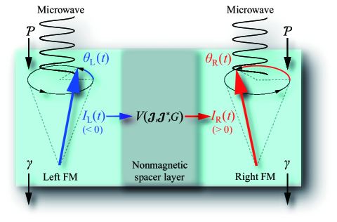
Figure 1: Magnonic $\varphi$ Josephson junction, formed by a ferromagnetic bilayer coupled by a non-magnetic spacer. Magnons are subjected to local damping at rate $\gamma>0$. The spacer layer-mediated interaction $V$ between the two FMs consists of coherent coupling (${\mathcal{J}}$) and non-local damping ($G$). Under microwave pumping, the spatially uniform mode of magnons is injected into each FM at rate $\mathcal{P}$, generating coherent spin precessions. The loss of magnons due to dissipation is exactly balanced by the injection of magnons. In the steady state, the spin precessions in each FM get synchronized due to non-local damping and a relative precession angle emerges $\varphi=\lim_{t\to\infty}[\theta_{\text{R}}(t)-\theta_{\text{L}}(t)]$ that depends on the magnon-magnon interaction. The associated magnon currents $I_{L,R}$ get rectified when $G\neq 0$.

Here, we fill this gap. We find that the inherent non-local damping leads to rich dynamics, and, interestingly, can be utilized to realize a magnonic analog of the $\varphi$ Josephson junction Bulaevskii et al. (1977); Geshkenbein et al. (1987); Sigrist and M. Rice (1992); Wollman et al. (1993); Van Harlingen (1995); Ryazanov et al. (2001); Il’ichev et al. (2001); Testa et al. (2004); Sickinger et al. (2012); Goldobin et al. (2013); Szombati et al. (2016); Tanaka and Kashiwaya (1996); Barash et al. (1996); Tanaka and Kashiwaya (1997); Mints (1998); Mints and Papiashvili (2001); Buzdin and Koshelev (2003); Gumann et al. (2007); Buzdin (2008); Goldobin et al. (2011). Under microwave pumping, coherent spin precession in each insulating ferromagnet (FM) of the magnetic junction (see Fig. 1) is synchronized by non-local damping as time advances and gives rise of a magnonic $\varphi$ Josephson junction, where $\varphi$ stands for the stationary value of the relative precession phase of the left and right FMs. Interestingly, we find that $\varphi$ decreases monotonically from $\pi$ to $\pi/2$ as the magnon-magnon interaction, arising from spin anisotropies across the junction, increases. Applying microwaves to each FM continuously, the junction reaches the nonequilibrium steady state where the loss of magnons due to dissipation is precisely balanced by the injection of magnons. Hence, spins in each FM continue to precess coherently, and the synchronized precession of the left and the right magnetization remains stable even at room temperature. Finally, we show that the magnetic junction exhibits rectification and acts as a diode for the magnon current.

II Magnonic Josephson junctions

We consider a magnetic junction, shown in Fig. 1, consisting of a bilayer of two insulating ferromagnetic layers, where the two FMs are separated by a nonmagnetic spacer layer, thereby weakly spin-exchange coupled. Applying microwaves to each FM and tuning the microwave frequency $\Omega>0$ of GHz to the magnon energy gap, ferromagnetic resonance is generated for each FM separately, where spins precess coherently. Under this microwave pumping, the zero wavenumber mode (i.e., spatially uniform mode) of magnons is excited and injected into each FM at the rate of $\mathcal{P}>0$ Nakata et al. (2015a). The magnons are subjected to local Gilbert damping at the rate $\gamma>0$ in each FM.

In addition, there is non-local damping Yu et al. (2024); Tserkovnyak (2020) that is mediated by the spacer interaction between the two FMs, see Fig. 1. Using the Holstein-Primakoff transformation Holstein and Primakoff (1940), this coupling term becomes to leading order Zou et al. (2024) $V=({\mathcal{J}}-i\hbar G/2)a_{\text{L}}^{\dagger}a_{\text{R}}+({\mathcal{J}}^{*}-i\hbar G/2)a_{\text{L}}a_{\text{R}}^{\dagger}$, where $a_{\text{L(R)}}^{(\dagger)}$ represents the magnon annihilation (creation) operator for the zero wavenumber mode, which satisfies the bosonic commutation relation. Here, ${\mathcal{J}}\in{\mathbb{C}}$, with its complex conjugate ${\mathcal{J}}^{*}$, describes coherent coupling, while $\hbar G\in{\mathbb{R}}$ describes the non-local damping (or dissipative coupling) Zou et al. (2024). The real part of coherent coupling, ${\text{Re}}({\mathcal{J}})={\mathcal{J}}_{\text{Re}}$, arises from the symmetric spin-exchange interaction between the two FMs, while its imaginary part Nakata et al. (2014, 2015a); Meier and Loss (2003); Serha et al. (2023), ${\text{Im}}({\mathcal{J}})={\mathcal{J}}_{\text{Im}}$, is induced, for example, by the Dzyaloshinskii-Moriya interaction when the spatial inversion symmetry of the nonmagnetic spacer layer is broken Katsura et al. (2005). Each component of ${\mathcal{J}}/\hbar$ can reach MHz in experiments Liang et al. (2023); Kammerbauer et al. (2023). The values of $\gamma$ and $G$ are typically within the MHz regime Heinrich et al. (2003), and the condition, $\hbar\Omega\gg|\mathcal{J}|,\hbar\gamma,|\hbar G|$, is satisfied. The condition $|G|\leq 2\gamma$ ensures the complete positivity of the system dynamics Zou et al. (2022, 2024, 2023), and we focus on this regime henceforth. We note that the coupling term $V$ becomes non-Hermitian due to non-local damping, i.e., $V\neq V^{\dagger}$ for $G\neq 0$.

The magnon-magnon interaction in the left (right) FM, $U_{\text{L(R)}}$, arises from anisotropies of spin, where $U_{\text{L}}=({U}/{2})a_{\rm{L}}^{\dagger}a_{\rm{L}}^{\dagger}a_{\rm{L}}a_{\rm{L}}$, $U_{\text{R}}=({U}/{2})a_{\text{R}}^{\dagger}a_{\text{R}}^{\dagger}a_{\text{R}}a_{\text{R}}$. Here, $U$ can take both positive and negative values, depending on the combination of anisotropies such as the spin anisotropy along the quantization axis and the anisotropy of the spin-exchange interaction in each FM Nakata et al. (2014, 2015a).

In this study, we envisage to continuously apply microwaves to each FM, which results in spins exhibiting macroscopic coherent precession characterized as $\langle a_{\text{L(R)}}(t)\rangle\neq 0$ Nakata et al. (2015a). Therefore, assuming a macroscopic coherent magnon state, thereby using the semiclassical approximation, we replace the operators $a_{\text{L}}(t)$ and $a_{\text{R}}(t)$ by their expectation values as $\langle a_{\text{L}}(t)\rangle=\sqrt{N_{\text{L}}(t)}{\text{e}}^{i\theta_{\text{L}}(t)}$ and $\langle a_{\text{R}}(t)\rangle=\sqrt{N_{\text{R}}(t)}{\text{e}}^{i\theta_{\text{R}}(t)}$, respectively, where $N_{\text{L(R)}}(t)>0$ represents the number of coherent magnons for each site in the left (right) FM and $\theta_{\text{L(R)}}$ is the phase (see Fig. 1). Defining the relative precession phase as $\theta(t)=\theta_{\text{R}}(t)-\theta_{\text{L}}(t)$, each time evolution [e.g., ${\dot{\theta}}(t)$ represents the time derivative of $\theta(t)$] is described as (see the Supplemental Material (SM) for details NHJ )

$${\dot{\theta}}(t)=\frac{{\mathcal{J}}_{\text{Re}}}{\hbar}\cos\theta(t)\left(\sqrt{\frac{N_{\text{R}}(t)}{N_{\text{L}}(t)}}-\sqrt{\frac{N_{\text{L}}(t)}{N_{\text{R}}(t)}}\right)+\sin\theta(t)\left[\left(\frac{{\mathcal{J}}_{\text{Im}}}{\hbar}+\frac{G}{2}\right)\sqrt{\frac{N_{\text{L}}(t)}{N_{\text{R}}(t)}}-\left(\frac{{\mathcal{J}}_{\text{Im}}}{\hbar}-\frac{G}{2}\right)\sqrt{\frac{N_{\text{R}}(t)}{N_{\text{L}}(t)}}\right]+u[N_{\text{L}}(t)-N_{\text{R}}(t)],$$ (1a)

$${\dot{N}}_{\text{L/R}}(t)=-2\gamma N_{\text{L/R}}(t)\pm 2\left[\frac{{\mathcal{J}}_{\text{Re}}}{\hbar}\sin\theta(t)+\left(\frac{{\mathcal{J}}_{\text{Im}}}{\hbar}\mp\frac{G}{2}\right)\cos\theta(t)\right]\sqrt{N_{\text{L}}(t)N_{\text{R}}(t)}+{\mathcal{P}},$$ (1b)

where $u=U/\hbar$. The second term on the right-hand side of Eq. (1b) describes the nonmagnetic spacer layer-mediated transport of coherent magnons in the junction.

The transport of coherent magnons in this junction is analogous to the Josephson effect Josephson (1962) in the sense that the current arises as the term of the order of $V$, $O(V)$, for the interaction $V=V({\mathcal{J}},{\mathcal{J}}^{*},G)$ between the two FMs (see Fig. 1) and is characterized by the relative precession phase $\theta(t)$. For these reasons Katsura et al. (2005), we refer to the transport of coherent magnons and the junction as the magnonic Josephson effect and the magnonic Josephson junction, respectively. Note that, in contrast, the current for incoherent magnons arises from a term of $O(V^{2})$ Nakata et al. (2015b, 2017).

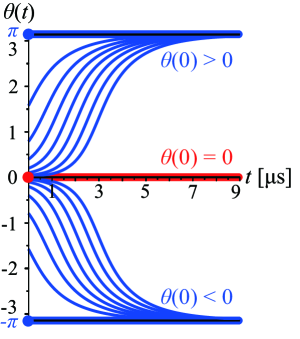
Figure 2: Plots of the relative phase $\theta(t)$ as a function of time in the absence of the magnon-magnon interaction, i.e., $u=0$, for the initial condition $\theta(0)=0$ and $|\theta(0)|=\pi/2^{n}$ with $n=0,1,...,7$ obtained by numerically solving Eqs. (3a)-(3c) for the parameter values ${\mathcal{J}}_{\text{Re}}=0$, ${\mathcal{J}}_{\text{Im}}/\hbar=G/2=0.5$ MHz, $\gamma=1.1$ MHz, ${\mathcal{P}}=2\gamma=2.2$ MHz, and $N_{\text{L}}(0)=N_{\text{R}}(0)=10^{-6}$. As time advances, coherent spin precession in each FM is synchronized and forms the magnonic $\pi$ Josephson junction as $\varphi=\theta(t\to\infty)=\pm\pi$ for $\theta(0)\neq 0$. The initial condition $\theta(0)=0$ for $u=0$ results in $\varphi=0$.

III Synchronized precession

To seek for a junction setup that exhibits synchronization and rectification effects, we consider the case where

$${\mathcal{J}}_{\text{Re}}=0\ \ \text{and}\ \ {\mathcal{J}}_{\text{Im}}/\hbar=G/2>0.$$ (2)

Under these assumptions, Eqs. (1a)-(1b) become

$${\dot{\theta}}(t)=G\sqrt{N_{\text{L}}/N_{\text{R}}}\sin\theta+u[N_{\text{L}}-N_{\text{R}}],$$ (3a)

$${\dot{N}}_{\text{L}}=-2\gamma N_{\text{L}}+{\mathcal{P}},$$ (3b)

$${\dot{N}}_{\text{R}}=-2\gamma N_{\text{R}}-2G\sqrt{N_{\text{L}}N_{\text{R}}}\cos\theta+{\mathcal{P}},$$ (3c)

where we suppressed for brevity the explicit time-dependence of the quantities $\theta(t)$ and $N_{\text{L/R}}(t)$. Under microwave pumping $\mathcal{P}$, the nonequilibrium steady state ${\dot{\theta}}(t)={\dot{N}}_{\text{L}}(t)={\dot{N}}_{\text{R}}(t)=0$ is realized, where $\theta(t)$, $N_{\text{L}}(t)$, and $N_{\text{R}}(t)$ approach their stationary values as time advances, i.e., $\varphi=\theta(t\to\infty)$ and $N_{\text{L(R)}}(t\to\infty)=N_{\text{L(R)}}^{\infty}$. Using Eqs. (3a)-(3c), we find the following relations between these asymptotic quantities:

$$\cos\varphi=(\gamma/G)(N_{\text{L}}^{\infty}-N_{\text{R}}^{\infty})/\sqrt{N_{\text{R}}^{\infty}N_{\text{L}}^{\infty}},$$ (4a)

$$\tan\varphi=-uN_{\text{R}}^{\infty}/{\gamma},$$ (4b)

where $N_{\text{L}}^{\infty}=\mathcal{P}/2\gamma$ is a constant, while $N_{\text{R}}^{\infty}$ becomes a function of the relative precession phase $\varphi$. In what follows, we will show that there is a unique solution to the system of Eqs. (4a) and (4b). Thereby, a magnonic analog of the $\varphi$ Josephson junction Bulaevskii et al. (1977); Geshkenbein et al. (1987); Sigrist and M. Rice (1992); Wollman et al. (1993); Van Harlingen (1995); Ryazanov et al. (2001); Il’ichev et al. (2001); Testa et al. (2004); Sickinger et al. (2012); Goldobin et al. (2013); Szombati et al. (2016); Tanaka and Kashiwaya (1996); Barash et al. (1996); Tanaka and Kashiwaya (1997); Mints (1998); Mints and Papiashvili (2001); Buzdin and Koshelev (2003); Gumann et al. (2007); Buzdin (2008); Goldobin et al. (2011) is realized.

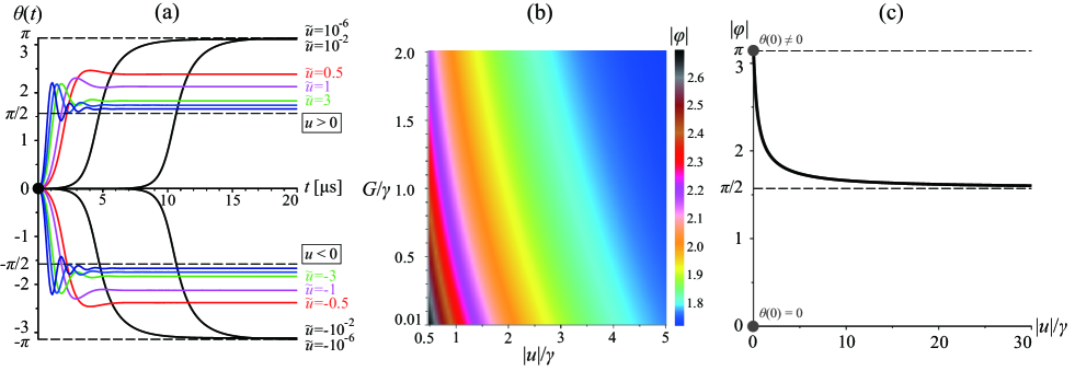
Figure 3: (a) Plots of the relative phase $\theta(t)$ as a function of time for several values of $\tilde{u}$ obtained by numerically solving Eqs. (3a)-(3c) for the same parameter values as in Fig. 2 as well as for $\theta(0)=0$. The stationary relative phase, $\varphi=\theta(t\to\infty)$, decreases from $|\varphi|=\pi$ to $|\varphi|=\pi/2$ as the magnon-magnon interaction $|\tilde{u}|$ increases, where we set $|\tilde{u}|=10^{-6},10^{-2},0.5,1,3,5,10$. We note that ${\text{sgn}}(\varphi)={\text{sgn}}(u)$. (b,c) The relative phase $|\varphi|$ decreases as $|u|/\gamma$ and $G/\gamma$ increase. These plots are obtained by numerically solving Eq. (5) for the same parameter values as in Fig. 3(a). (c) Plot of $|\varphi|$ as a function of $|u|/\gamma$, showing that $|\varphi|$ decreases monotonically from $\pi$ to $\pi/2$ as $|u|/\gamma$ increases. For $u\neq 0$, the value of $|\varphi|$ does not depend on the initial conditions. For $u=0$, $|\varphi|$ depends on the initial condition $\theta(0)$ as $|\varphi|=\pi$ for $\theta(0)\neq 0$, whereas $\varphi=0$ for $\theta(0)=0$ (see Fig. 2).

III.1 Absence of magnon interaction: $u=0$

First, we study the behavior of $\varphi$ in the absence of the magnon-magnon interaction, $u=0$. From Eq. (4b), we immediately find that $\varphi$ can only be equal to $\pm\pi$ or $0$. One of these three values is chosen based on the initial condition $\theta(0)$. Figure 2 shows the plots of the relative phase $\theta(t)$ for several initial conditions $\theta(0)$ as a function of time obtained by numerically solving Eqs. (3a)-(3c). If $\theta(0)=0$, the relative phase stays constant, $\theta(t)=0$. If the symmetry is broken, i.e., $\theta(0)\neq 0$, we have $\varphi=\pi\ \rm{sgn}\ \theta(0)$. This shows that the coherent spin precessions in each FM get synchronized with each other as time advances. This asymptotic locking of the spin precessions is a direct consequence of the dissipative coupling term $G$. The junction behavior represents a magnonic analog of the well-known $\pi$ Josephson junction effect in superconductors Bulaevskii et al. (1977); Geshkenbein et al. (1987); Sigrist and M. Rice (1992); Wollman et al. (1993); Van Harlingen (1995); Ryazanov et al. (2001).

Figure 2 also shows that the point $\theta(0)=0$ is unstable in the sense that $\varphi=0$ for the initial condition $\theta(0)=0$, whereas $\varphi=\pm\pi$ for $\theta(0)\neq 0$. However, to realize such a special condition, $\theta(0)=0$ with $u=0$, will be out of experimental reach. Moreover, in what follows, we will show that any finite value of $u$ results in $\varphi\neq 0$, no matter what initial value we choose for $\theta(0)$ including the fine-tuned value $\theta(0)=0$, see Fig. 3.

We emphasize that our results are independent of the initial values $N_{\text{L}}(0)$ and $N_{\text{R}}(0)$ and do not depend on the assumption that both FMs are pumped at the same rate $\mathcal{P}$. A detailed discussion is available in the SM NHJ . We also remark that the synchronized precession of the left and the right magnetization, ${\dot{\theta}}(t)=0$, remains valid even if the parameter values slightly deviate from Eq. (2). See the SM NHJ for the plots, where it is shown numerically that, although the value of $\varphi$ slightly changes depending on the magnitude of the deviation, the synchronized precession is robust against such perturbations. We note that under the initial condition $\theta(0)=0$, we have $\varphi\neq 0$ for ${\mathcal{J}}_{\text{Re}}\neq 0$, whereas $\varphi=0$ for ${\mathcal{J}}_{\text{Re}}=0$. Also in this sense, the point $\theta(0)=0$ is unstable. See the SM NHJ for more details.

III.2 Finite magnon interaction: $u\neq 0$

Next, we study the behavior of $\varphi$ in the presence of the magnon-magnon interaction, $u\neq 0$, and determine $\varphi$ as a function of $u$. First, from Eq. (4b), we deduce that $\varphi(u)$ is an odd function of $u$, i.e., $\varphi(u)=-\varphi(-u)$ (mod $2\pi$). Here, we used that $N_{\text{R}}^{\infty}(\varphi)=N_{\text{R}}^{\infty}(-\varphi)$, which follows from Eq. (4a). In Fig. 3, we solve numerically Eqs. (3a)-(3c) and confirm that $\varphi(u)$ is odd. Remarkably, even if the initial condition is chosen as $\theta(0)=0$, for $u\neq 0$, the magnitude of $\varphi$ monotonically decreases from $|\varphi|=\pi$ to $|\varphi|=\pi/2$ as the magnitude of the magnon-magnon interaction increases. We note that this condition is consistent with the requirement that the direction of magnon propagation in the junction, see Fig. 1, is chosen to be from left to right (see also below).

Introducing the rescaled magnon-magnon interaction ${\tilde{u}}=(u/\gamma)N_{\text{L}}^{\infty}$ and combining Eqs. (3a)-(3c), we get the following implicit equation on $\tan\varphi$:

$$\tan^{4}\varphi+2\tilde{u}\tan^{3}\varphi+(1+{\tilde{u}}^{2})\tan^{2}\varphi$$

$$\hskip 60.0pt+\left[2+\left(G/\gamma\right)^{2}\right]{\tilde{u}}\tan\varphi+{\tilde{u}}^{2}=0,$$ (5)

whose solution gives us $\varphi$ as function of ${\tilde{u}}$. For $\varphi\in[-\pi,\pi]$, there are generally four solutions for $\varphi$. The two solutions with $\cos\varphi>0$ are excluded as they will result in an unphysical direction of the current $I_{R}$ that is set by the nonlocal interaction term $V$ (see below). Finally, one more solution is eliminated as it breaks the condition $\tan\varphi<-\tilde{u}$, which follows from Eqs. (4a) and (4b) for $\tilde{u}>0$. That leaves us with a unique solution for $\varphi$.

In Fig. 3(b), we investigate $|\varphi|$ as a function of both $|u|/\gamma$ and $G/\gamma$ by numerically solving Eq. (5). For a given $\tilde{u}$ ($G$), $|\varphi|$ decreases monotonically from $\pi$ to $\pi/2$ as $G$ ($\tilde{u}$) increases, see Fig. 3(b,c). The asymptotic expressions for $\varphi$ for the two limiting cases of weak and strong interactions can be obtained also analytically. Indeed, from Eqs. (5) and (4a) and for strong interactions, $\tilde{u}\gg 1$, we get in leading order in $1/{\tilde{u}}$

$$\varphi\simeq\pi/2+1/\tilde{u},$$ (6a)

$$N_{\text{R}}^{\infty}/N_{\text{L}}^{\infty}\simeq 1+G/\tilde{u}\gamma.$$ (6b)

In the opposite limit of weak interactions, $0<\tilde{u}\ll 1$, we obtain, keeping leading corrections in $\tilde{u}$ in each quantity,

$$\varphi\simeq\pi-c{\tilde{u}},$$ (7a)

$$N_{\text{R}}^{\infty}/N_{\text{L}}^{\infty}\simeq c\left(1-G(c\tilde{u})^{2}/\sqrt{G^{2}+4\gamma^{2}}\right)$$ (7b)

where $c=(\sqrt{1+\left(G/2\gamma\right)^{2}}+G/2\gamma)^{2}$. These equations together with Fig. 3(c) are one of the main results of this study. Remarkably, both limiting values for $\varphi$, namely $\pi/2$ and $\pi$, are obviously universal, i.e., independent of any material properties as well as of initial conditions. This underlines the robust and universal property of the synchronization of precessions brought about by the nonlocal damping in magnetic junctions driven by microwaves.

IV Rectification

The magnonic $\varphi$ Josephson junction can be regarded as a magnonic analog of the Josephson diode Zhang et al. (2022); Davydova et al. (2022); Wu et al. (2022), in the sense that it exhibits a rectification effect for the magnon currents, as we will show next. From Eq. (1b) one gets that the current of coherent magnons that flows from the nonmagnetic spacer layer into the left (right) FM (see Fig. 1), $I_{\text{L(R)}}(t)=O(V)$, is given by

$$I_{\text{L/R}}= \pm 2\Big{[}\frac{{\mathcal{J}}_{\text{Re}}}{\hbar}\sin\theta+\Big{(}\frac{{\mathcal{J}}_{\text{Im}}}{\hbar}\mp\frac{G}{2}\Big{)}\cos\theta\Big{]}\sqrt{N_{\text{L}}N_{\text{R}}},$$ (8)

in units of $g\mu_{\text{B}}$ for the $g$-factor $g$ of the constituent spins, and where we suppressed for brevity the explicit time-dependence of the quantities $\theta(t)$ and $N_{\text{L/R}}(t)$. The condition specified in Eq. (2) results in

$$I_{\text{L}}(t)= 0,$$ (9a)

$$I_{\text{R}}(t)= -2G\sqrt{N_{\text{L}}(t)N_{\text{R}}(t)}\cos\theta.$$ (9b)

Since the nonequilibrium steady state is realized under microwave pumping $\mathcal{P}$, the current $I_{\text{R}}(t)$ continues to flow while keeping the rectification effect characterized by $I_{\text{L}}(t)=0$ in the magnonic $\varphi$ Josephson junction (see Fig. 1). We emphasize that the rectification of the magnon current holds also in the presence of the magnon-magnon interaction.

Note that our analytical solutions for $\varphi$ must satisfy $\cos\varphi<0$ and thus the magnitude of $\varphi$ is bounded as ${\pi}/{2}<|\varphi|\leq\pi$ to ensure $\lim_{t\to\infty}I_{\text{R}}(t)\geq 0$. We recall that the non-local damping $G$ provides the non-Hermitian property to the nonmagnetic spacer layer-mediated interaction described by $V$. Under the special conditions stated in Eq. (2) one gets $V=-i\hbar Ga_{\text{L}}a_{\text{R}}^{\dagger}$. This shows that propagation of magnons becomes chiral and is allowed only in the direction from left to right in the junction. This is consistent with the sign choice of the current and its direction as shown in Fig. 1.

In the absence of non-local damping, $G=0$, the current of coherent magnons propagates in both directions through the nonmagnetic spacer layer, from the left to the right FM and vice versa Nakata et al. (2014). This results in $I_{\text{R}}(t)=-I_{\text{L}}(t)$ for $G=0$ [see Eqs. (8)]. Thus, we see that rectification only occurs in the presence of non-local damping when $G\neq 0$.

If instead of Eq. (2), one uses the condition

$${\mathcal{J}}_{\text{Re}}=0\ \ \text{and}\ \ {\mathcal{J}}_{\text{Im}}/\hbar=-G/2,$$ (10)

we get from Eq. (8) that

$$I_{\text{L}}(t)= -2G\sqrt{N_{\text{L}}(t)N_{\text{R}}(t)}\cos\theta(t),$$ (11a)

$$I_{\text{R}}(t)= 0.$$ (11b)

Thus, the rectification effect changes its direction. We conclude that the polarity of the rectification effect is determined by the sign of $G$.

V Experimental feasibility

The key ingredient for the magnonic Josephson effect is the coherent magnon state $\langle a_{\text{L(R)}}(t)\rangle\neq 0$ (i.e., coherent spin precession), and it can be realized through microwave pumping Nakata et al. (2015a). Since each component of coherent coupling ${\mathcal{J}}$ is tunable by adjusting the thickness of the nonmagnetic spacer layer Parkin et al. (1990, 1991); Husain et al. (2022); Yun et al. (2023) or applying an electric field Srivastava et al. (2018); Fillion et al. (2022); Koyama et al. (2018); Vedmedenko et al. (2019), the magnonic $\varphi$ Josephson junction is realizable by tuning coherent coupling appropriately. Moreover, applying microwave to each FM continuously, the loss of magnons due to dissipation is precisely balanced by the injection of magnons achieved through microwave pumping. Therefore, spins in each FM continue to precess coherently, and the synchronized precession of the magnonic $\varphi$ Josephson junctions remains stable. Thus, our theoretical prediction is within experimental reach with current device and measurement techniques through magnetization measurement.

VI Conclusion

We have investigated the effect of non-local damping on magnetic junctions and found that it serves as the key ingredient for the synchronized precession and gives rise to a magnonic $\varphi$ Josephson junction. The spacer layer-mediated interaction between the two FMs in the junctions consists of coherent coupling and non-local damping, and it becomes non-Hermitian due to non-local damping. Tuning them appropriately, coherent spin precession in each FM is synchronized by non-local damping as time advances and forms a $\varphi$ Josephson junction, where the relative precession angle $\varphi$ decreases monotonically from $|\varphi|=\pi$ to $|\varphi|=\pi/2$ as the magnitude of the magnon-magnon interaction increases, with both limiting values being entirely universal. The magnon currents in the junction exhibits rectification and gives rise to a magnonic diode effect. Applying microwaves to each FM continuously, the junction reaches the nonequilibrium steady state where the loss of magnons due to dissipation is precisely balanced by the injection of magnons achieved through microwave pumping. Hence, spins in each FM continue to precess coherently, and the synchronized precession of the left and the right magnetization remains stable.

Supplemental Material for “Magnonic $\varphi$ Josephson Junctions and Synchronized Precession”

In this Supplemental Material, we provide details on the derivation of the magnonic Josephson equations, on the equation for $\varphi$ as a function of the magnon-magnon interaction, and on the parameter dependence of our results.

Appendix S-I Magnonic Josephson equations

In this section, we provide details on the derivation of the magnonic Josephson equations. The effective non-Hermitian Hamiltonian ${\mathcal{H}}$ for the magnonic Josephson junction is given as Zou et al. (2024); Nakata et al. (2014, 2015a) ${\mathcal{H}}={\mathcal{H}}_{\text{L}}+{\mathcal{H}}_{\text{R}}+V+U_{\text{L}}+U_{\text{R}}$ with (see also main text) ${\mathcal{H}}_{\text{L}}=\hbar(\Omega-i\gamma)a_{\text{L}}^{\dagger}a_{\text{L}}$ and ${\mathcal{H}}_{\text{R}}=\hbar(\Omega-i\gamma)a_{\text{R}}^{\dagger}a_{\text{R}}$, where $a_{\text{L(R)}}^{(\dagger)}$ represents the magnon annihilation (creation) operator for the zero wavenumber mode (i.e., spatially uniform mode) in the left (right) FM. This provides the time evolution of each operator as

$$i\hbar{\dot{a}}_{\text{L}}(t)= \hbar(\Omega-i\gamma)a_{\text{L}}(t)+({\mathcal{J}}-i\hbar G/2)a_{\text{R}}(t)+Ua_{\text{L}}^{\dagger}(t)a_{\text{L}}(t)a_{\text{L}}(t),$$ (S12a)

$$i\hbar{\dot{a}}_{\text{R}}(t)= \hbar(\Omega-i\gamma)a_{\text{R}}(t)+({\mathcal{J}}^{*}-i\hbar G/2)a_{\text{L}}(t)+Ua_{\text{R}}^{\dagger}(t)a_{\text{R}}(t)a_{\text{R}}(t).$$ (S12b)

Here, assuming a macroscopic coherent magnon state, thereby using the semiclassical approximation, we replace the operators $a_{\text{L}}(t)$ and $a_{\text{R}}(t)$ by their expectation values as $\langle a_{\text{L}}(t)\rangle=\sqrt{N_{\text{L}}(t)}{\text{e}}^{i\theta_{\text{L}}(t)}$ and $\langle a_{\text{R}}(t)\rangle=\sqrt{N_{\text{R}}(t)}{\text{e}}^{i\theta_{\text{R}}(t)}$, respectively, where $N_{\text{L(R)}}(t)\in{\mathbb{R}}$ represents the number of coherent magnons for each site in the left (right) FM and $\theta_{\text{L(R)}}(t)\in{\mathbb{R}}$ is the phase. Defining the relative phase as

$$\theta(t)=\theta_{\text{R}}(t)-\theta_{\text{L}}(t),$$ (S13)

Eqs. (S12a) and (S12b) for $N_{\text{L(R)}}(t)\neq 0$ become

$$i\hbar\Big{(}\frac{1}{2}\frac{{\dot{N}}_{\text{L}}}{N_{\text{L}}}+i{\dot{\theta}}_{\text{L}}\Big{)} =\hbar(\Omega-i\gamma)+UN_{\text{L}}+\Big{[}{\mathcal{J}}_{\text{Re}}+i\Big{(}{\mathcal{J}}_{\text{Im}}-\frac{\hbar}{2}G\Big{)}\Big{]}\sqrt{\frac{N_{\text{R}}}{N_{\text{L}}}}{\text{e}}^{i\theta},$$ (S14a)

$$i\hbar\Big{(}\frac{1}{2}\frac{{\dot{N}}_{\text{R}}}{N_{\text{R}}}+i{\dot{\theta}}_{\text{R}}\Big{)} =\hbar(\Omega-i\gamma)+UN_{\text{R}}+\Big{[}{\mathcal{J}}_{\text{Re}}-i\Big{(}{\mathcal{J}}_{\text{Im}}+\frac{\hbar}{2}G\Big{)}\Big{]}\sqrt{\frac{N_{\text{L}}}{N_{\text{R}}}}{\text{e}}^{-i\theta},$$ (S14b)

where ${\text{Re}}({\mathcal{J}})={\mathcal{J}}_{\text{Re}}\in{\mathbb{R}}$ and ${\text{Im}}({\mathcal{J}})={\mathcal{J}}_{\text{Im}}\in{\mathbb{R}}$. Real and imaginary parts of Eqs. (S14a) and (S14b) provide

$$-\hbar{\dot{\theta}}_{\text{L}} =\hbar\Omega+UN_{\text{L}}+\Big{[}{\mathcal{J}}_{\text{Re}}\cos\theta-\Big{(}{\mathcal{J}}_{\text{Im}}-\frac{\hbar}{2}G\Big{)}\sin\theta\Big{]}\sqrt{\frac{N_{\text{R}}}{N_{\text{L}}}},$$ (S15a)

$$\frac{\hbar}{2}\frac{{\dot{N}}_{\text{L}}}{N_{\text{L}}} =-\hbar\gamma+\Big{[}{\mathcal{J}}_{\text{Re}}\sin\theta+\Big{(}{\mathcal{J}}_{\text{Im}}-\frac{\hbar}{2}G\Big{)}\cos\theta\Big{]}\sqrt{\frac{N_{\text{R}}}{N_{\text{L}}}},$$ (S15b)

$$-\hbar{\dot{\theta}}_{\text{R}} =\hbar\Omega+UN_{\text{R}}+\Big{[}{\mathcal{J}}_{\text{Re}}{{\cos}}\theta-\Big{(}{\mathcal{J}}_{\text{Im}}+\frac{\hbar}{2}G\Big{)}\sin\theta\Big{]}\sqrt{\frac{N_{\text{L}}}{N_{\text{R}}}},$$ (S15c)

$$\frac{\hbar}{2}\frac{{\dot{N}}_{\text{R}}}{N_{\text{R}}} =-\hbar\gamma-\Big{[}{\mathcal{J}}_{\text{Re}}\sin\theta+\Big{(}{\mathcal{J}}_{\text{Im}}+\frac{\hbar}{2}G\Big{)}\cos\theta\Big{]}\sqrt{\frac{N_{\text{L}}}{N_{\text{R}}}},$$ (S15d)

where Eq. (S15a) is the real part of Eq. (S14a), Eq. (S15b) is the imaginary part of Eq. (S14a), Eq. (S15c) is the real part of Eq. (S14b), and Eq. (S15d) is the imaginary part of Eq. (S14b). Taking the difference between Eqs. (S15a) and (S15c), those are rewritten as

$${\dot{\theta}}(t)= \frac{{\mathcal{J}}_{\text{Re}}}{\hbar}\cos\theta\Big{(}\sqrt{\frac{N_{\text{R}}}{N_{\text{L}}}}-\sqrt{\frac{N_{\text{L}}}{N_{\text{R}}}}\Big{)}+\sin\theta\Big{[}\Big{(}\frac{{\mathcal{J}}_{\text{Im}}}{\hbar}+\frac{G}{2}\Big{)}\sqrt{\frac{N_{\text{L}}}{N_{\text{R}}}}-\Big{(}\frac{{\mathcal{J}}_{\text{Im}}}{\hbar}-\frac{G}{2}\Big{)}\sqrt{\frac{N_{\text{R}}}{N_{\text{L}}}}\Big{]}+u(N_{\text{L}}-N_{\text{R}}),$$ (S16a)

$${\dot{N}}_{\text{L}}(t)= -2\gamma N_{\text{L}}+2\Big{[}\frac{{\mathcal{J}}_{\text{Re}}}{\hbar}\sin\theta+\Big{(}\frac{{\mathcal{J}}_{\text{Im}}}{\hbar}-\frac{G}{2}\Big{)}\cos\theta\Big{]}\sqrt{N_{\text{L}}N_{\text{R}}},$$ (S16b)

$${\dot{N}}_{\text{R}}(t)= -2\gamma N_{\text{R}}-2\Big{[}\frac{{\mathcal{J}}_{\text{Re}}}{\hbar}\sin\theta+\Big{(}\frac{{\mathcal{J}}_{\text{Im}}}{\hbar}+\frac{G}{2}\Big{)}\cos\theta\Big{]}\sqrt{N_{\text{L}}N_{\text{R}}}.$$ (S16c)

In this study, we assume to continuously apply microwaves to each FM. The coherent magnon state, the key ingredient for the magnonic Josephson effect, is realized by microwave pumping. Under microwave pumping, coherent magnons are injected into each FM at the rate of $\mathcal{P}$ Nakata et al. (2015a). Taking this effect of the magnon injection through microwave pumping into account, Eqs. (S16b) and (S16c) become

$${\dot{N}}_{\text{L}}(t)= -2\gamma N_{\text{L}}+2\Big{[}\frac{{\mathcal{J}}_{\text{Re}}}{\hbar}\sin\theta+\Big{(}\frac{{\mathcal{J}}_{\text{Im}}}{\hbar}-\frac{G}{2}\Big{)}\cos\theta\Big{]}\sqrt{N_{\text{L}}N_{\text{R}}}+\mathcal{P},$$ (S17a)

$${\dot{N}}_{\text{R}}(t)= -2\gamma N_{\text{R}}-2\Big{[}\frac{{\mathcal{J}}_{\text{Re}}}{\hbar}\sin\theta+\Big{(}\frac{{\mathcal{J}}_{\text{Im}}}{\hbar}+\frac{G}{2}\Big{)}\cos\theta\Big{]}\sqrt{N_{\text{L}}N_{\text{R}}}+\mathcal{P}.$$ (S17b)

Finally, the magnonic Josephson equations under microwave pumping in the presence of non-local damping are summarized as

$${\dot{\theta}}(t)= \frac{{\mathcal{J}}_{\text{Re}}}{\hbar}\cos\theta(t)\Big{(}\sqrt{\frac{N_{\text{R}}(t)}{N_{\text{L}}(t)}}-\sqrt{\frac{N_{\text{L}}(t)}{N_{\text{R}}(t)}}\Big{)}+\sin\theta(t)\Big{[}\Big{(}\frac{{\mathcal{J}}_{\text{Im}}}{\hbar}+\frac{G}{2}\Big{)}\sqrt{\frac{N_{\text{L}}(t)}{N_{\text{R}}(t)}}-\Big{(}\frac{{\mathcal{J}}_{\text{Im}}}{\hbar}-\frac{G}{2}\Big{)}\sqrt{\frac{N_{\text{R}}(t)}{N_{\text{L}}(t)}}\Big{]}+u[N_{\text{L}}(t)-N_{\text{R}}(t)],$$ (S18a)

$${\dot{N}}_{\text{L}}(t)= -2\gamma N_{\text{L}}(t)+2\Big{[}\frac{{\mathcal{J}}_{\text{Re}}}{\hbar}\sin\theta(t)+\Big{(}\frac{{\mathcal{J}}_{\text{Im}}}{\hbar}-\frac{G}{2}\Big{)}\cos\theta(t)\Big{]}\sqrt{N_{\text{L}}(t)N_{\text{R}}(t)}+{\mathcal{P}},$$ (S18b)

$${\dot{N}}_{\text{R}}(t)= -2\gamma N_{\text{R}}(t)-2\Big{[}\frac{{\mathcal{J}}_{\text{Re}}}{\hbar}\sin\theta(t)+\Big{(}\frac{{\mathcal{J}}_{\text{Im}}}{\hbar}+\frac{G}{2}\Big{)}\cos\theta(t)\Big{]}\sqrt{N_{\text{L}}(t)N_{\text{R}}(t)}+{\mathcal{P}}.$$ (S18c)

Appendix S-II Dynamics with different pumping rates

In this section, we consider the scenario where $\mathcal{J}_{\text{Re}}=0$, $\mathcal{J}_{\text{Im}}/\hbar=G/2$, and $u=0$, with different pumping rates for two FMs. By solving the dynamics analytically, we demonstrate that our results do not rely on the initial conditions.

Let us first only pump the left FM with rate $\mathcal{P}$. In this case, the coupled dynamics is governed by the following equations:

$$\dot{\theta}(t) =G\sqrt{\frac{N_{\text{L}}}{N_{\text{R}}}}\sin\theta,$$ (S19)

$$\dot{N}_{\text{L}} =-2\gamma N_{\text{L}}+\mathcal{P},$$

$$\dot{N}_{\text{R}} =-2\gamma N_{\text{R}}-2G\sqrt{N_{\text{L}}N_{\text{R}}}\cos\theta.$$

We now solve these equations analytically. We first introduce $n_{{\text{L}}/{\text{R}}}(t)=e^{2\gamma t}N_{{\text{L}}/{\text{R}}}(t)$, which allows us to rewrite the equations into the following form:

$$\dot{n}_{\text{L}}=e^{2\gamma t}\mathcal{P},\;\;\dot{\theta}=G\sqrt{\frac{n_{\text{L}}}{n_{\text{R}}}}\sin\theta,\;\;\dot{n}_{\text{R}}=-2G\sqrt{n_{\text{R}}n_{\text{L}}}\cos\theta.$$ (S20)

The first equation can be solved:

$$n_{\text{L}}(t)=N_{\text{L}}(0)+\frac{\mathcal{P}}{2\gamma}(e^{2\gamma t}-1).$$ (S21)

The last two equations leads to

$$\derivative{\theta}{n_{\text{R}}}=-\frac{1}{2}\frac{\tan\theta}{n_{\text{R}}}\longrightarrow|\sin\theta(t)|\sqrt{n_{\text{R}}(t)}=|\sin\theta(0)|\sqrt{N_{\text{R}}(0)}.$$ (S22)

We then obtain the equation for $\theta(t)$ under the initial condition $\theta(0)\neq 0$ and $\theta(0)\neq\pm\pi$:

$$\derivative{\theta}{t}=\frac{G\sqrt{n_{\text{L}}(t)}}{|\sin\theta(0)|\sqrt{N_{\text{R}}(0)}}\sin\theta|\sin\theta|.$$ (S23)

We point out that the above equation can be solved analytically since the integral of $\sqrt{n_{\text{L}}(t)}$ can be performed analytically. But we will focus on the case where $t\gg 1/(2\gamma)$ so $n_{\text{L}}(t)\approx(\mathcal{P}/2\gamma)e^{2\gamma t}$ for our purpose.

Let us also focus on the case of $\sin\theta(0)>0$ and look for the solution that satisfies $\sin\theta(t)>0$. One can similarly solve for the case when $\sin\theta(0)<0$. We have:

$$\tan\theta(t)=\frac{1}{\cot\theta(0)-\alpha e^{\gamma t}}\longrightarrow\theta(t)=\arctan\left[\frac{1}{\cot\theta(0)-\alpha e^{\gamma t}}\right],$$ (S24)

where $\alpha$ is a constant:

$$\alpha\equiv\frac{(G/\gamma)\sqrt{\mathcal{P}/(2\gamma)}}{\sin\theta(0)\sqrt{N_{\text{R}}(0)}}.$$ (S25)

In the large $t\rightarrow\infty$ limit, we can drop $\cot\theta(0)$ in the expression. Then the expression of $\theta(t)$ is reduced to:

$${\theta(t)=\pi-\frac{1}{\alpha}e^{-\gamma t}.}$$ (S26)

One can also easily write down the expression of $n_{\text{R}}(t)$:

$${\sqrt{n_{\text{R}}(t)}=\alpha|\sin\theta(0)|\sqrt{N_{\text{R}}(0)}e^{2\gamma t}.}$$ (S27)

At large $t\rightarrow\infty$, we have

$${\sqrt{\frac{N_{\text{R}}^{\infty}}{N_{\text{L}}^{\infty}}}=\frac{G}{\gamma}.}$$ (S28)

It is interesting to note that this final value is independent of the initital condition and also the pumping rate $\mathcal{P}$.

Finally, when we pump the two FMs at the same time, the physics is very similar to the case that we discussed above. The only difference is that $N_{\text{R}}^{\infty}$ is different. The equations are given by

$$\dot{\theta}(t) =G\sqrt{\frac{N_{\text{L}}}{N_{\text{R}}}}\sin\theta,$$ (S29)

$$\dot{N}_{\text{L}} =-2\gamma N_{\text{L}}+\mathcal{P}_{\text{L}},$$

$$\dot{N}_{\text{R}} =-2\gamma N_{\text{R}}-2G\sqrt{N_{\text{L}}N_{\text{R}}}\cos\theta+\mathcal{P}_{\text{R}}.$$

Here $\mathcal{P}_{\text{L}}$ and $\mathcal{P}_{\text{R}}$ are the pumping rates of the two FMs. We introduce the ratio

$$\beta\equiv\sqrt{\frac{N_{\text{R}}^{\infty}}{N_{\text{L}}^{\infty}}}.$$ (S30)

Then it is determined by the equation

$$\beta^{2}-\frac{G}{\gamma}\beta-\frac{\mathcal{P}_{\text{R}}}{\mathcal{P}_{\text{L}}}=0\longrightarrow\beta=\frac{G/\gamma+\sqrt{(G/\gamma)^{2}+4\mathcal{P}_{\text{R}}/\mathcal{P}_{\text{L}}}}{2},$$ (S31)

at $t\rightarrow\infty$. Here, let us again focus on the case of $\sin\theta(0)>0$ and look for the solution that satisfies $\sin\theta(t)>0$. Similar to our previous conclusion, $\theta(t)$ also approaches $\pi$ exponentially fast but now with a different exponent:

$${\pi-\theta(t)\propto e^{-(G/\beta)t}.}$$ (S32)

Note that in the absence of the pumping of the right FM $\mathcal{P}_{\text{R}}=0$, we have $\beta=G/\gamma$ and $\pi-\theta(t)\propto e^{-\gamma t}$, which is what we obtained before.

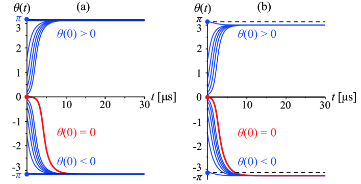
Figure S1: Plots of the relative phase $\theta(t)$ as a function of time in the absence of the magnon-magnon interaction, i.e., $u=0$, for the initial condition $\theta(0)=0$ and $|\theta(0)|=\pi/2^{n}$ with $n=0,1,...,5$ obtained by numerically solving Eqs. (S18a)-(S18c). The parameter values are the same as in Fig. 2 of the main text, e.g., $G=1$ MHz, except for (a) $C_{1}=C_{2}=10$ kHz and (b) $C_{1}=100$ kHz and $C_{2}=10$ kHz. Even in the presence of such perturbation $C_{1(2)}$, the synchronized precession of the left and the right magnetization, ${\dot{\theta}}(t)=0$, remains valid. The value of $\varphi$ slightly changes depending on the magnitude of the deviation ($C_{1}$ and $C_{2}$). Under the initial condition $\theta(0)=0$, it becomes $\varphi\neq 0$ for $C_{1}\neq 0$, whereas $\varphi=0$ for $C_{1}=0$ (see Fig. 2). Also in this sense, the point $\theta(0)=0$ is instable.

Appendix S-III Robustness of synchronized precession

In the main text, to seek for the junction that exhibits a rectification effect characterized by $I_{\text{L}}(t)=0$, we consider the case

$${\mathcal{J}}_{\text{Re}}=0\ \ \text{and}\ \ {\mathcal{J}}_{\text{Im}}/\hbar=G/2>0.$$ (S33)

In this section, although the rectification effect ceases to work and it becomes $I_{\text{L}}(t)\neq 0$, we numerically show that the synchronized precession of the left and the right magnetization, ${\dot{\theta}}(t)=0$, remains valid even if the parameter values slightly deviate from Eq. (S33). For this, we consider a case with

$${\mathcal{J}}_{\text{Re}}/\hbar=C_{1}\ \ \text{and}\ \ {\mathcal{J}}_{\text{Im}}/\hbar=G/2+C_{2},$$ (S34)

where each constant $C_{1(2)}$ satisfies $|C_{1(2)}|\ll G$. Figure S1 shows that the synchronized precession of the left and the right magnetization is robust against such perturbation $C_{1(2)}$.

Appendix S-IV Nonequilibrium steady state for finite magnon interaction

In this section, we provide details on the derivation of the equation for $\varphi$ as a function of the magnon-magnon interaction. For

$${\mathcal{J}}_{\text{Re}}=0\ \ \text{and}\ \ {\mathcal{J}}_{\text{Im}}/\hbar=G/2,$$ (S35)

Eqs. (S18a)-(S18c) become

$${\dot{\theta}}(t)= G\sqrt{\frac{N_{\text{L}}(t)}{N_{\text{R}}(t)}}\sin\theta(t)+u[N_{\text{L}}(t)-N_{\text{R}}(t)],$$ (S36a)

$${\dot{N}}_{\text{L}}(t)= -2\gamma N_{\text{L}}(t)+{\mathcal{P}},$$ (S36b)

$${\dot{N}}_{\text{R}}(t)= -2\gamma N_{\text{R}}(t)-2G\sqrt{N_{\text{L}}(t)N_{\text{R}}(t)}\cos\theta(t)+{\mathcal{P}}.$$ (S36c)

Under microwave pumping $\mathcal{P}$, the nonequilibrium steady state ${\dot{\theta}}(t)={\dot{N}}_{\text{L}}(t)={\dot{N}}_{\text{R}}(t)=0$ is realized, where $\theta(t)$, $N_{\text{L}}(t)$, and $N_{\text{R}}(t)$ approach asymptotically to time-independent constant as time advances, $\varphi=\lim_{t\to\infty}\theta(t)$ and $N_{\text{L,R}}^{\infty}=\lim_{t\to\infty}N_{\text{L,R}}(t)$. Thus, from Eqs. (S36a),  (S36b) and (S36c), for $u\neq 0$, we get

$$N_{\text{L}}^{\infty}-N_{\text{R}}^{\infty}=-\frac{G}{u}\sqrt{\frac{N_{\text{L}}^{\infty}}{N_{\text{R}}^{\infty}}}\sin\varphi,$$ (S37a)

$$N_{\text{L}}^{\infty}=\frac{\mathcal{P}}{2\gamma},$$ (S37b)

$$N_{\text{L}}^{\infty}-N_{\text{R}}^{\infty}=\frac{G}{\gamma}\sqrt{N_{\text{L}}^{\infty}N_{\text{R}}^{\infty}}\cos\varphi,$$ (S37c)

From Eq. (S37c), we get the ratio between the number of coherent magnons in the left and right FMs,

$$\sqrt{\frac{N_{\text{R}}^{\infty}}{N_{\text{L}}^{\infty}}}=\sqrt{1+\left(\frac{G}{2\gamma}\cos\varphi\right)^{2}}-\frac{G}{2\gamma}\cos\varphi.$$ (S38)

Combining Eq. (S37a) and Eq. (S37c), we obtain

$$\tan\varphi=-\frac{u}{\gamma}N_{\text{R}}^{\infty},$$ (S39)

$$(N_{\text{L}}^{\infty}-N_{\text{R}}^{\infty})^{2}=-\frac{G^{2}}{\gamma u}N_{\text{L}}^{\infty}\frac{\sin(2\varphi)}{2}.$$ (S40)

If $u>0$, the solution exists only for $\tan\varphi<0$. Substituting $N_{\text{R}}^{\infty}$ from Eq.  (S39) into Eq. (S40), we arrive at the implicit equation for $\tan\varphi$:

$$\Big{(}\frac{\gamma}{u}\tan\varphi+N_{\text{L}}^{\infty}\Big{)}^{2}=-\frac{G^{2}}{\gamma u}N_{\text{L}}^{\infty}\frac{\tan\varphi}{1+\tan^{2}\varphi}.$$ (S41)

This equation can be brought into the form of a quartic equation displayed in the main text:

$$\tan^{4}\varphi+2\tilde{u}\tan^{3}\varphi+(1+{\tilde{u}}^{2})\tan^{2}\varphi+\left[2+\left(\frac{G}{\gamma}\right)^{2}\right]{\tilde{u}}\tan\varphi+{\tilde{u}}^{2}=0,$$ (S42)

where we introduced the rescaled dimensionless magnon-magnon interaction parameter ${\tilde{u}}=(u/\gamma)N_{\text{L}}^{\infty}$. We note that the solution is possible only for $\tan\varphi<0$ ($\tan\varphi>0$) for $u>0$ ($u<0$). We note that for a quartic polynomial one can find an explicit solution. However, it is too involved to be displayed here. In the main text we give the analytical expressions for $\varphi$ for the limiting cases of small and large ${\tilde{u}}$.

References

- Ashida et al. (2020) Y. Ashida, Z. Gong, and M. Ueda, Adv. Phys. 69, 249 (2020), arXiv:2006.01837 .
- Chumak et al. (2015) A. V. Chumak, V. I. Vasyuchka, A. A. Serga, and B. Hillebrands, Nat. Phys. 11, 453 (2015).
- Chumak et al. (2022) A. V. Chumak, P. Kabos, M. Wu, C. Abert, C. Adelmann, A. Adeyeye, J. Åkerman, F. G. Aliev, A. Anane, A. Awad, et al., IEEE Trans. Magn. 58, 1 (2022), arXiv:2111.00365 .
- Yuan et al. (2022) H. Yuan, Y. Cao, A. Kamra, R. A. Duine, and P. Yan, Phys. Rep. 965, 1 (2022), arXiv:2111.14241 .
- Nakata et al. (2014) K. Nakata, K. A. van Hoogdalem, P. Simon, and D. Loss, Phys. Rev. B 90, 144419 (2014), arXiv:1406.7004 .
- Troncoso and Núñez (2014) R. E. Troncoso and Á. S. Núñez, Ann. Phys. (N. Y.) 346, 182 (2014), arXiv:1305.4285 .
- Liu et al. (2016) Y. Liu, G. Yin, J. Zang, R. K. Lake, and Y. Barlas, Phys. Rev. B 94, 094434 (2016), arXiv:1605.09427 .
- Khymyn et al. (2017) R. Khymyn, I. Lisenkov, V. Tiberkevich, B. A. Ivanov, and A. Slavin, Sci. Rep. 7, 43705 (2017), arXiv:1609.09866 .
- Yu et al. (2024) T. Yu, J. Zou, B. Zeng, J. Rao, and K. Xia, Phys. Rep. 1062, 1 (2024), arXiv:2306.04348 .
- Tserkovnyak (2020) Y. Tserkovnyak, Phys. Rev. Res. 2, 013031 (2020), arXiv:1911.01619 .
- Zou et al. (2024) J. Zou, S. Bosco, E. Thingstad, J. Klinovaja, and D. Loss, Phys. Rev. Lett. 132, 036701 (2024), arXiv:2306.15916 .
- Bulaevskii et al. (1977) L. Bulaevskii, V. Kuzii, and A. Sobyanin, J. Exp. Theor. Phys. Lett. 25, 290 (1977).
- Geshkenbein et al. (1987) V. B. Geshkenbein, A. I. Larkin, and A. Barone, Phys. Rev. B 36, 235 (1987).
- Sigrist and M. Rice (1992) M. Sigrist and T. M. Rice, J. Phys. Soc. Jpn. 61, 4283 (1992).
- Wollman et al. (1993) D. A. Wollman, D. J. Van Harlingen, W. C. Lee, D. M. Ginsberg, and A. J. Leggett, Phys. Rev. Lett. 71, 2134 (1993).
- Van Harlingen (1995) D. J. Van Harlingen, Rev. Mod. Phys. 67, 515 (1995).
- Ryazanov et al. (2001) V. V. Ryazanov, V. A. Oboznov, A. Y. Rusanov, A. V. Veretennikov, A. A. Golubov, and J. Aarts, Phys. Rev. Lett. 86, 2427 (2001), arXiv:cond-mat/0008364 .
- Il’ichev et al. (2001) E. Il’ichev, M. Grajcar, R. Hlubina, R. P. J. IJsselsteijn, H. E. Hoenig, H.-G. Meyer, A. Golubov, M. H. S. Amin, A. M. Zagoskin, A. N. Omelyanchouk, and M. Y. Kupriyanov, Phys. Rev. Lett. 86, 5369 (2001), arXiv:cond-mat/0102404 .
- Testa et al. (2004) G. Testa, A. Monaco, E. Esposito, E. Sarnelli, D.-J. Kang, S. Mennema, E. Tarte, and M. Blamire, Appl. Phys. Lett. 85, 1202 (2004).
- Sickinger et al. (2012) H. Sickinger, A. Lipman, M. Weides, R. G. Mints, H. Kohlstedt, D. Koelle, R. Kleiner, and E. Goldobin, Phys. Rev. Lett. 109, 107002 (2012), arXiv:1207.3013 .
- Goldobin et al. (2013) E. Goldobin, H. Sickinger, M. Weides, N. Ruppelt, H. Kohlstedt, R. Kleiner, and D. Koelle, Appl. Phys. Lett. 102, 242602 (2013), arXiv:1306.1683 .
- Szombati et al. (2016) D. Szombati, S. Nadj-Perge, D. Car, S. Plissard, E. Bakkers, and L. Kouwenhoven, Nat. Phys. 12, 568 (2016), arXiv:1512.01234 .
- Tanaka and Kashiwaya (1996) Y. Tanaka and S. Kashiwaya, Phys. Rev. B 53, R11957 (1996).
- Barash et al. (1996) Y. S. Barash, H. Burkhardt, and D. Rainer, Phys. Rev. Lett. 77, 4070 (1996).
- Tanaka and Kashiwaya (1997) Y. Tanaka and S. Kashiwaya, Phys. Rev. B 56, 892 (1997).
- Mints (1998) R. G. Mints, Phys. Rev. B 57, R3221 (1998).
- Mints and Papiashvili (2001) R. G. Mints and I. Papiashvili, Phys. Rev. B 64, 134501 (2001), arXiv:cond-mat/0101085 .
- Buzdin and Koshelev (2003) A. Buzdin and A. E. Koshelev, Phys. Rev. B 67, 220504 (2003), arXiv:cond-mat/0305142 .
- Gumann et al. (2007) A. Gumann, C. Iniotakis, and N. Schopohl, Appl. Phys. Lett. 91, 192502 (2007), arXiv:0708.3898 .
- Buzdin (2008) A. Buzdin, Phys. Rev. Lett. 101, 107005 (2008), arXiv:0808.0299 .
- Goldobin et al. (2011) E. Goldobin, D. Koelle, R. Kleiner, and R. G. Mints, Phys. Rev. Lett. 107, 227001 (2011), arXiv:1110.2326 .
- Nakata et al. (2015a) K. Nakata, P. Simon, and D. Loss, Phys. Rev. B 92, 014422 (2015a), arXiv:1502.03865 .
- Holstein and Primakoff (1940) T. Holstein and H. Primakoff, Phys. Rev. 58, 1098 (1940).
- Meier and Loss (2003) F. Meier and D. Loss, Phys. Rev. Lett. 90, 167204 (2003), arXiv:cond-mat/0209521 .
- Serha et al. (2023) R. O. Serha, V. I. Vasyuchka, A. A. Serga, and B. Hillebrands, Phys. Rev. B 108, L220404 (2023), arXiv:2312.05113 .
- Katsura et al. (2005) H. Katsura, N. Nagaosa, and A. V. Balatsky, Phys. Rev. Lett. 95, 057205 (2005), arXiv:cond-mat/0412319 .
- Liang et al. (2023) S. Liang, R. Chen, Q. Cui, Y. Zhou, F. Pan, H. Yang, and C. Song, Nano Lett. 23, 8690 (2023).
- Kammerbauer et al. (2023) F. Kammerbauer, W.-Y. Choi, F. Freimuth, K. Lee, R. Frmter, D.-S. Han, R. Lavrijsen, H. J. Swagten, Y. Mokrousov, and M. Klui, Nano Lett. 23, 7070 (2023).
- Heinrich et al. (2003) B. Heinrich, Y. Tserkovnyak, G. Woltersdorf, A. Brataas, R. Urban, and G. E. W. Bauer, Phys. Rev. Lett. 90, 187601 (2003), arXiv:cond-mat/0210588 .
- Zou et al. (2022) J. Zou, S. Zhang, and Y. Tserkovnyak, Phys. Rev. B 106, L180406 (2022), arXiv:2108.07365 .
- Zou et al. (2023) J. Zou, S. Bosco, and D. Loss, (2023), arXiv:2308.03054 .
- (42) See Supplemental Material for the derivation of the magnonic Josephson equations, for that of the equation for as a function of the magnon-magnon interaction, and for the parameter dependence of our results.
- Josephson (1962) B. D. Josephson, Phys. Lett. 1, 251 (1962).
- Nakata et al. (2015b) K. Nakata, P. Simon, and D. Loss, Phys. Rev. B 92, 134425 (2015b), arXiv:1507.03807 .
- Nakata et al. (2017) K. Nakata, P. Simon, and D. Loss, J. Phys. D: Appl. Phys. 50, 114004 (2017), arXiv:1610.08901 .
- Zhang et al. (2022) Y. Zhang, Y. Gu, P. Li, J. Hu, and K. Jiang, Phys. Rev. X 12, 041013 (2022), arXiv:2112.08901 .
- Davydova et al. (2022) M. Davydova, S. Prembabu, and L. Fu, Sci. Adv. 8, eabo0309 (2022), arXiv:2201.00831 .
- Wu et al. (2022) H. Wu, Y. Wang, Y. Xu, P. K. Sivakumar, C. Pasco, U. Filippozzi, S. S. Parkin, Y.-J. Zeng, T. McQueen, and M. N. Ali, Nature 604, 653 (2022), arXiv:2103.15809 .
- Parkin et al. (1990) S. S. P. Parkin, N. More, and K. P. Roche, Phys. Rev. Lett. 64, 2304 (1990).
- Parkin et al. (1991) S. S. P. Parkin, R. Bhadra, and K. P. Roche, Phys. Rev. Lett. 66, 2152 (1991).
- Husain et al. (2022) S. Husain, S. Pal, X. Chen, P. Kumar, A. Kumar, A. K. Mondal, N. Behera, N. K. Gupta, S. Hait, R. Gupta, R. Brucas, B. Sanyal, A. Barman, S. Chaudhary, and P. Svedlindh, Phys. Rev. B 105, 064422 (2022).
- Yun et al. (2023) J. Yun, B. Cui, Q. Cui, X. He, Y. Chang, Y. Zhu, Z. Yan, X. Guo, H. Xie, J. Zhang, et al., Adv. Funct. Mater. , 2301731 (2023).
- Srivastava et al. (2018) T. Srivastava, M. Schott, R. Juge, V. Krizakova, M. Belmeguenai, Y. Roussigné, A. Bernand-Mantel, L. Ranno, S. Pizzini, S.-M. Chérif, et al., Nano Lett. 18, 4871 (2018).
- Fillion et al. (2022) C.-E. Fillion, J. Fischer, R. Kumar, A. Fassatoui, S. Pizzini, L. Ranno, D. Ourdani, M. Belmeguenai, Y. Roussigné, S.-M. Chérif, et al., Nat. Commun. 13, 5257 (2022), arXiv:2204.04031 .
- Koyama et al. (2018) T. Koyama, Y. Nakatani, J. Ieda, and D. Chiba, Sci. Adv. 4, eaav0265 (2018).
- Vedmedenko et al. (2019) E. Y. Vedmedenko, P. Riego, J. A. Arregi, and A. Berger, Phys. Rev. Lett. 122, 257202 (2019), arXiv:1803.10570 .