Discrete Newtonian dynamics with Nosé-Hoover thermostats

Abstract

Almost all Molecular Dynamics (MD) simulations are discrete dynamics with Newton’s algorithm first published in 1687, and much later by L. Verlet in 1967. Discrete Newtonian dynamics has the same qualities as Newton’s classical analytic dynamics. Verlet also published a first-order expression for the instant temperature which is inaccurate but presumably used in most MD simulations. One of the motivations for the present article is to correct this unnecessary inaccuracy in $NVT$ MD dynamics. Another motivation is to derive simple algorithms for the Nosé-Hoover $NVT$ dynamics (NH) with the correct temperature constraint. The simulations with NH discrete Newtonian dynamics show that the NH works excellent for a wide range of the response time $\tau$ of the NH thermostat, but NH simulations favor a choice of a short response time, even shorter than the discrete time increment $\delta t$ used in MD, to avoid large oscillations of the temperature.

I Introduction

Newton published PHILOSOPHIÆ NATURALIS PRINCIPIA MATHEMATICA ($Principia$) in 1687 Newton1687 ; Toxvaerd2023 and he began $Principia$ by postulating the discrete Newtonian dynamics in Proposition I, where he used the algorithm for discrete dynamics to derive his second law for classical mechanics. The classical analytic dynamics of $N$ interacting objects is the exact solution, obtained by solving the coupled second-order analytic differential equations for the accelerations of the objects. The exact analytic solution for the dynamical evolution of the positions of the objects is characterized by being time-reversible and symplectic, and by having three invariances for a conservative system: the conservation of momentum, angular momentum, and the energy of the system. But Newton’s discrete dynamics is also time reversible and symplectic and has the same three invariances Toxvaerd2023 , and if the exactness of classical mechanics is given by these five qualities, then his discrete dynamics is also exact. Furthermore, there exists a shadow Hamiltonian where discrete positions are located on the analytical trajectories for the shadow Hamiltonian Toxvaerd2023 ; Toxvaerd1994 ; Toxvaerd2012 . This means that there is no qualitative difference between Newton’s analytic and discrete dynamics.

The discrete Newtonian algorithm was much later in 1967 rediscovered by Loop Verlet Verlet1967 and used in his pioneering Molecular Dynamics (MD) simulation of a system of Lennard-Jones particles. The algorithm has been reformulated several times and appears under a variety of names, the most well-known is the Leapfrog version. Almost all MD simulations today in Natural Science are performed by Newton’s discrete algorithm. A review of the discrete Newtonian dynamics is given in reference No.2 Toxvaerd2023 with the proofs of the invariances for a conservative system. The proof of the conservation of the energy is also given here in the appendix.

Loop Verlet also derived a first-order expression $\textbf{v}_{0,i}(t)$ for the discrete velocity $\textbf{v}_{i}(t)$ for object No. $i$ at time $t$ obtained by a symmetric Taylor expansion Toxvaerd2023appendix

$$\textbf{v}_{i}(t)=\textbf{v}_{0,i}(t)-\frac{1}{6}\frac{\delta t^{2}}{m_{i}}\textbf{f}_{i}^{\prime}(t)+\mathcal{O}(\delta t^{4}\textbf{f}_{i}^{\prime\prime\prime}(t))$$ (1)

with

$$\textbf{v}_{0,i}(t)=\frac{\textbf{r}_{i}(t+\delta t)-\textbf{r}_{i}(t-\delta t)}{2\delta t}$$ (2)

from its positions $\textbf{r}_{i}(t-\delta t)$ and $\textbf{r}_{i}(t+\delta t)$, and this expression is used in today’s MD Tildesley ; Frenkel . The velocity $\textbf{v}_{0,i}(t)$ in Eq. (2) is the first term for the velocity in Verlet’s forward and backward Taylor expansion of the discrete position $\textbf{r}(t)$, and if the velocity is approximated by this expression, it entails a systematic and sometimes significant error in the calculated temperature and in the heat capacity of a system Toxvaerd2023a . It is the one of the reasons for this article, where the correct expression for the velocity and the kinetic energy is used to revise the formulation of the $NVT$ Nosé-Hoover algorithm (NH) for $NVT$ simulations Hoover1985 . Constant temperature MD has been simulated for many decades and the method is reviewed in Harish2021 . Many of the algorithms for discrete dynamics at constant temperatures are, however, with broken time symmetry and irreversible dynamics. However, the NH dynamics, which is derived from the steady state Lioville equation for an extended phase space with friction with a friction coefficient $\eta(t)$, is time reversible Hoover1985 ; Hoover1991 .

The article starts in Section 2 by presenting the expressions for the velocities, kinetic energy, and temperature by the use of the energy invariance derived in the appendix, and the NH algorithms for $NVT$ discrete dynamics are presented in Section 3. The algorithms are used in Section 4 to obtain $NVT$ state points for a system of Lennard-Jones particles (LJ). Section 5 summarizes the results.

II Discrete Newtonian dynamics

The classical discrete dynamics between $N$ spherically symmetrical objects with masses $m^{N}=m_{1},m_{2},..m_{i},..,m_{N}$ and positions r${}^{N}(t)=$r${}_{1}(t)$, r${}_{2}(t),..,$r${}_{i}(t),..$r${}_{N}(t)$ is obtained by Newton’s discrete algorithm. Let the force, $\textbf{f}_{i}$ on object No. $i$ be a sum of pairwise forces $\textbf{f}_{ij}$ between pairs of objects $i$ and $j$

$$\textbf{f}_{i}=\sum_{j\neq i}^{N}\textbf{f}_{ij}.$$ (3)

Newton’s discrete algorithm is a symmetrical time-centered difference whereby the dynamics is time reversible and symplectic. The Verlet formulation of the algorithm is

$$\textbf{r}_{i}(t+\delta t)=2\textbf{r}_{i}(t)-\textbf{r}_{i}(t-\delta t)+\frac{\delta t^{2}}{m_{i}}\textbf{f}_{i}(i).$$ (4)

The energy in analytic dynamics is the sum of potential energy $U(\textbf{r}^{N}(t))$ and kinetic energy $K(t)$, and it is an invariance for a conservative system with analytic dynamics. There is, however, a problem with the determination of the kinetic energy in the discrete dynamics since the velocities at time $t$ are not known. Traditionally one uses Eq. (2) and the expressions

$$K_{0}(t)=\sum_{i}^{N}\frac{1}{2}m_{i}\textbf{v}_{0,i}(t)^{2}$$ (5)

$$E_{0}(t)=U(\textbf{r}^{N}(t))+K_{0}(t)$$ (6)

for the velocity, kinetic energy $K(t)$, potential energy $U(\textbf{r}^{N}(t))$ and energy $E(t)$ in MD. But the total energy $E_{0}$ obtained by using Eq. (6) with $K(t)=K_{0}(t)$ for the kinetic energy fluctuates with time although it remains constant, averaged over long time intervals. This is due to the fundamental quality of Newton’s discrete dynamics, where the positions and momenta appear asynchronous and with a discrete change in momentum at time $t$. The energy invariance in discrete Newtonian dynamics (D) is derived in the appendix. The kinetic energy $K_{D}(t)$ in the time interval $[t-\delta t/2,t+\delta t/2]$ is

$$K_{\textrm{D}}=\frac{1}{2}(K_{\textrm{D}_{+}}+K_{\textrm{D}_{-}})=$$

$$=\frac{1}{2}\sum_{i}^{N}\frac{1}{2}m_{i}[\frac{\textbf{(}\textbf{r}_{i}(t+\delta t)-\textbf{r}_{i}(t))^{2}}{\delta t^{2}}+\frac{\textbf{(}\textbf{r}_{i}(t)-\textbf{r}_{i}(t-\delta t))^{2}}{\delta t^{2}}]$$

$$=\frac{1}{2}\sum_{i}^{N}\frac{1}{2}m_{i}(\textbf{v}_{i}(t+\delta t/2)^{2}+\textbf{v}_{i}(t-\delta t/2)^{2}).$$ (7)

II.1 The temperature in discrete Newtonian dynamics

The constant kinetic energies in the time intervals $[t-\delta t/2,t]$ and $[t,t+\delta t/2]$ in between a force impulse at time $t$ are related Toxvaerd2013 . It is easy to derive the relation

$$\textbf{v}_{0,i}(t)^{2}=\frac{1}{2}\textbf{v}_{i}(t+\delta t/2)^{2}+\frac{1}{2}\textbf{v}_{i}(t-\delta t/2)^{2}-\frac{1}{4}(\delta t/m_{i}\textbf{f}_{i}(t))^{2}$$ (8)

from Eq. (4) between the first-order expression Eq. (2) for the square of the velocity at time $t$ and the well-defined expression for the square of the velocities $\textbf{v}_{i}(t-\delta t/2)$ and $\textbf{v}_{i}(t+\delta t/2)$ in the time intervals $[t-\delta t/2,t]$ and $[t,t+\delta t/2]$. The corresponding expression for the kinetic energy, $K_{0}(t)$, and the traditional value for the temperature used in MD simulations

$$k_{\textrm{B}}T_{0}(t)=\frac{<2K_{0}(t)>}{N_{f}}$$ (9)

used in MD simulations for a system with $N_{f}$ degrees of freedom is less than the mean kinetic energy, $K_{D}(t)$, and the temperature

$$k_{\textrm{B}}T_{\textrm{D}}(t)=\frac{<2K_{D}(t)>}{N_{f}}.$$ (10)

In the discrete time interval $[t-\delta t/2,t+\delta t/2]$ the relation is

$$K_{0}(t)=K_{D}(t)-\sum_{i}^{N}\frac{1}{8}\delta t^{2}/m_{i}\textbf{f}_{i}(t)^{2}.$$ (11)

The correct temperature $T_{D}$ is bigger than $T_{0}$ and the difference between $T_{D}$ and $T_{0}$ increases with density, temperature, and the discrete time step $\delta t$. The difference is relatively small and of the order of a few percent at state points with low pressure, but it is significant for state points with high densities, pressure, temperatures, the strength of the repulsive forces, or for large time increments $\delta t$ Toxvaerd2023a .

III NVT ensemble simulations with the Nosé-Hoover thermostats

Many NVT ensemble simulations in MD are with the Nosé-Hoover thermostat (NH-MD) where a friction $\eta(t)\textbf{p}_{i}(t)$ acts simultaneously with the force $\textbf{f}_{i}(t)$ Hoover1985 . The Hamilton formulation of classical dynamics with the friction is Hoover1985 ; Hoover1991

$$\dot{\textbf{r}}_{i}(t)=\textbf{p}_{i}(t)$$ (12)

$$\dot{\textbf{p}}_{i}(t)=\textbf{f}_{i}(t)/m_{i}-\eta(t)\textbf{p}_{i}(t)$$ (13)

$$\dot{\eta}(t)=\alpha^{-1}(K(t)-K),$$ (14)

with a restoring friction $\eta(t)\textbf{p}_{i}(t)$ which constrains the kinetic energy $K(t)$ to $K=2N_{f}k_{\textrm{B}}T$. The damping factor $\alpha$ is expressed as

$$\alpha=N_{f}\tau/2,$$ (15)

where $\tau$ is a characteristic ”response” time of the thermostat Toxvaerd1991 .

The discrete Newtonian dynamics with the time symmetrical Leapfrog formulation with NH-MD is

$$\textbf{r}_{i}(t+\delta t)=\textbf{r}_{i}(t)+\delta t\textbf{v}_{i}(t+\delta t/2)$$ (16)

$$\textbf{v}_{i}(t+\delta t/2)=\textbf{v}_{i}(t-\delta t/2)+\delta t/m_{i}\textbf{f}_{i}(t)$$

$$-\eta(t)(\textbf{v}_{i}(t+\delta t/2)+\textbf{v}_{i}(t-\delta t/2))/2,$$ (17)

and the discrete friction variable $\eta(t)$ can either be updated from two sets of discrete values $\eta(t-\delta t),\eta(t)$ by

$$\eta(t+\delta t)=\eta(t-\delta t)+\delta t/\tau(T_{D}(t)-T)\textrm{ Method I},$$ (18)

or by

$$\eta(t+\delta t)=\eta(t)+\delta t/\tau(T_{D_{+}}(t)-T)\textrm{ Method II},$$ (19)

where $k_{\textrm{B}}T_{D_{+}}=\sum_{i}^{N}m_{i}\textbf{v}(t+\delta t/2)^{2}/N_{f}$. Eq. (18) is the time centred analog to Newton’s discrete central difference algorithm. The time symmetry and time reversibility is maintained in the NH-MD discrete dynamics with both methods, and both methods have been used in NH-MD Toxvaerd1991 ; Hoover1990 .

The NH dynamics can be extended to include more than one thermostat and this has been used in simulations of systems with organic chain molecules. The thermostats can equilibrate specific modes in the systems or act on all $N_{f}$ degrees of freedom Frenkelchap6 . In the present formulation of NH dynamics and with $n$ thermostats which act with all $N_{f}$ modes

$$\eta_{1}(t+\delta t)=\eta_{1}(t-\delta t)+\delta t/\tau_{1}(T_{D}(t)-T)$$

$$\eta_{2}(t+\delta t)=\eta_{2}(t-\delta t)+\delta t/\tau_{2}(T_{D}(t)-T)$$

$$.........,$$ (20)

and with a total friction $\eta=\Sigma_{i}^{n}\eta_{i}/n$.

Eq. (17) can be rearranged to

$$\textbf{v}_{i}(t+\delta t/2)=\frac{\textbf{v}_{i}(t-\delta t/2)(1-\eta(t)/2)+\delta t/m_{i}\textbf{f}_{i}(t)}{1+\eta(t)/2},$$ (21)

and the $NVT$ time reversible NH-MD dynamics is obtained by the NH-MD algorithm: Eqn. (16) and (21) with either Eq. (18), and/or Eq. (19) , and/or Eq. (20).

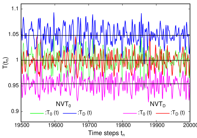
Figure 1: NH-MD with $T_{Thermostat}=T_{0}=1.00$ $(NVT_{0}$, old NH-MD), and with $T_{Thermostat}=T_{D}=1.00$ $(NVT_{D}$, present NH-MD). The figure shows five hundred (representative) time steps for the simulations of $10^{6}$ time steps. The temperatures $\bar{T}_{D}$ and the root mean square (rms) fluctuations are given in Table I.

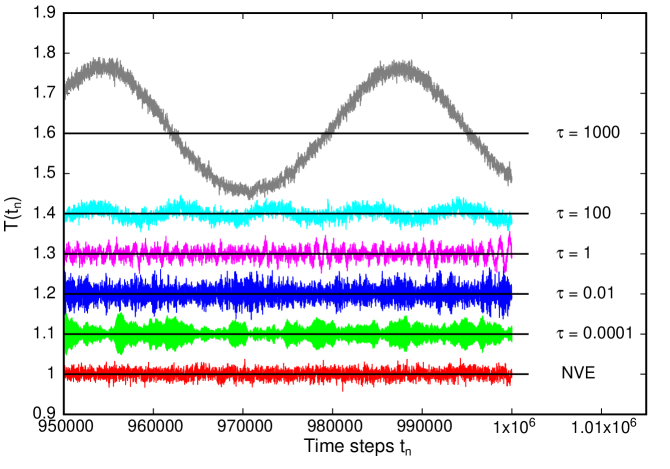
Figure 2: Five evolutions of $T_{D}(t)$ in a LJ system of $N=2000$ particles with $\delta t=0.005$ and with a NH thermostat with $T=1.0$ (Method I, Eq. (18)) together with the corresponding temperature without a thermostat (NVE). (Four NH-evolutions are parallel shifted with succeding $\Delta T=0.1$, and the last evolution with $\tau=1000$ is shifted with $\Delta T=0.2$.) All six simulations are started from the same NVE start configuration with different values of $\tau$. The figure shows the last 50000 time steps for the simulations of $10^{6}$ time steps. The temperatures $\bar{T}_{D}$ and the root mean square (rms) fluctuations are given in Table I.

Table 1: Temperatures in the LJ system.

$\tau$	$T_{D}\pm rms$	$T_{0}\pm rms$	$\eta\pm rms$	Method
-	1.000000000 $\pm 9.5\times 10^{-3}$	-	NVE
0.0001	0.999999993 $\pm 1.7\times 10^{-2}$	0.999014 $\pm 1.7\times 10^{-2}$	$-2.06\times 10^{-6}\pm 0.18$	I
0.0001	1.000000025 $\pm 1.8\times 10^{-2}$	0.999023 $\pm 1.8\times 10^{-2}$	$1.7\times 10^{-6}\pm 1.4\times 10^{-2}$	II
0.001	1.000000970$\pm 1.7\times 10^{-2}$	0.999025 $\pm 1.7\times 10^{-2}$	$-2.81\times 10^{-6}\pm 2.1\times 10^{-3}$	I
0.01	1.000000052$\pm 1.8\times 10^{-2}$	0.999024 $\pm 1.8\times 10^{-2}$	$2.39\times 10^{-6}\pm 2.1\times 0.1277$	I
0.1	0.999998637$\pm 1.8\times 10^{-2}$	0.999023 $\pm 1.8\times 10^{-2}$	$-1.68\times 10^{-6}\pm 4.0\times 10^{-2}$	I
1	1.000005194 $\pm 1.8\times 10^{-2}$	0.999030 $\pm 1.8\times 10^{-2}$	$3.76\times 10^{-7}\pm 1.3\times 10^{-2}$	I
1	0.999995501 $\pm 1.9\times 10^{-2}$	0.999029 $\pm 1.9\times 10^{-2}$	$-9.16\times 10^{-7}\pm 3.2\times 10^{-3}$	II
10	0.999986336 $\pm 1.9\times 10^{-2}$	0.999011 $\pm 1.7\times 10^{-2}$	$1.29\times 10^{-6}\pm 4.3\times 10^{-3}$	I
100	0.999883749 $\pm 2.9\times 10^{-2}$	0.998908 $\pm 2.9\times 10^{-2}$	$2.3\times 10^{-6}\pm 2.3\times 10^{-3}$	I
1000	0.999458904 $\pm 0.12108$	0.998477 $\pm 0.12083$	$1.73\times 10^{-5}\pm 3.2\times 10^{-3}$	I
1000	0.999516366 $\pm 0.1236$		$1.50\times 10^{-5}\pm 3.2\times 10^{-3}$	II

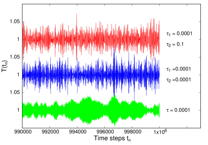
Figure 3: The temperature fluctuations of $T_{D}(t)$ in the temperature interval [0.95, 1.05] for NH-dynamics with one and with two thermostats. The fluctuations of the temperature with one thermostat and $\tau=0.0001$ are also shown in green in Figure 1. The fluctuations in the temperature interval [0.95, 1.05] with two thermostates are shown above, and for two sets of frictions. With red is for $\tau_{1}=0.0001$ and $\tau_{2}=0.1$. With blue is $T_{D}(t)$ with $\tau_{1}=\tau_{2}=0.0001$ with different start values of $\eta_{1}(0),\eta_{1}(-\delta t)$ and $\eta_{2}(0),\eta_{2}(-\delta t)$, respectively.

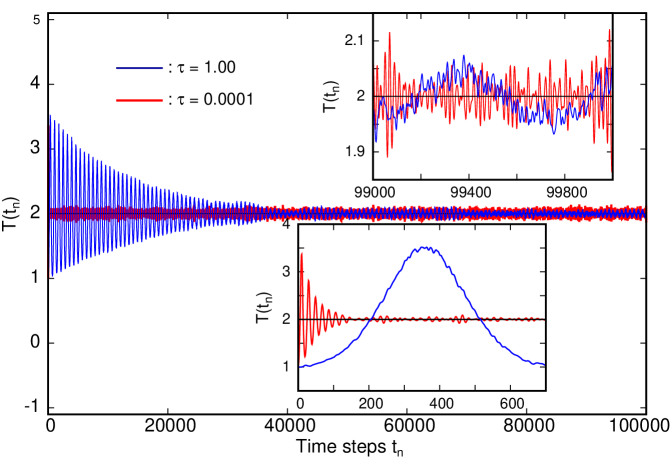
Figure 4: Temperature evolution in the LJ system by changing the thermostat temperature from $T_{1}=1.00$ to $T_{2}=2.00$. With blue is $T_{D}(t)$ for a relative long response time $\tau=1.00$ and with red is for a short response time $\tau=0.0001$. The lower inset shows the temperature evolution at the start of the calibration and the upper inset is at the end of the calibration of the temperature.

IV $NVT$ simulations

The Nosé-Hoover friction $\eta(t)$ thermostats the system’s instantaneous kinetic energy and temperature $T(t)$ using kinetic energy, Eq. (18) or Eq.(19). Most $NVT_{0}$ simulations with NH-MD use Verlet’s expression $T_{0}(t)$, Eq. (9), for the temperature. The exact expression for the kinetic energy and the instant temperature $T_{D}(t)$ by the discrete dynamics is, however systematically higher and given by Eq. (10). The difference between the two canonical simulations, $NVT_{0}$, and $NVT_{D}$, increases with the discrete time increment $\delta t$ and the force according to Eq. (8). It is of the order a few percent or less for many MD $NVE$ simulations at moderate densities and force fields Toxvaerd2023a , but can be much larger for stronger forces.

The differences between the two ensemble simulations, $NVT_{0}$ and $NVT_{D}$, where the instant temperature is either given by $T_{0}(t)$ or by $T_{D}(t)$, are determined for a Lennard-Jones system (LJ). The Lennard-Jones system is a simple model of a system with the classical gas-liquid-solid thermodynamic behavior. Systems of $N=2000$ LJ particles were simulated for various state points $\rho,T$. The differences between $NVT_{0}$ and $NVT_{D}$ at the high density $[\rho=1.40,T=1.00]$ fluid state point, and with $\delta t=0.010$ and $\tau=0.0010$ units are shown in Figure 1. The NH thermostat constrains a specified kinetic energy either to a given temperature $T$ by Eq. (9): $NVT_{0}$ with $T_{0}(t)=T$, or by Eq. (10): $NVT_{D}$ with $T_{D}(t)=T$. The mean canonical temperatures $\bar{T}_{0}$ and $\bar{T}_{D}$, respectively, are in both cases equal to the input temperature $T=1$, and in both cases the difference between $NVT_{0}$ and $NVT_{D}$, obtained from $10^{6}$ time steps are $\approx$ 4- 5 per cent. For $NVT_{0}$: $T_{0}=1.0000000$, green curve in Figure 1; $T_{D}=1.049$, blue curve. For $NVT_{D}$: $T_{D}=1.0000000$, red curve in Figure 1; $T_{0}=0.954$, magenta curve. (The figure shows the difference in a short time interval of five hundred steps).

IV.1 Nosé-Hoover simulations of a Lennard-Jones system

The two NH algorithms for $NVT$ dynamics ( I and II) are tested by MD simulations of a LJ system with the thermostats at various state points in the fluid state of the LJ system. The first examples are for a liquid state point $(T,\rho)=(1,0.60)$ near the coexisting liquid with the density $\rho_{l}=0.589$ at $T=1.00$ Watanabe2012 . The temperatures $T_{D}(t)$ for various values of the NH-response time $\tau$ are shown in Figure 2, and the mean temperatures and their root mean fluctuations are given in Table I. The thermostats work excellent for a wide range of the values of the response time $\tau$ but the system’s instant temperature $T_{D}(t)$ exhibits oscillations for values of the response time $\tau>>1$, whereas the thermostat works excellent for smaller values, and even for response times $\tau<\delta t$.

Table I contains also data for NH dynamics with Method II for $\tau=0.0001,1$ and 1000, respectively, and there are no differences between the mean temperatures obtained by the two algorithms. The thermostats were tested for different temperatures and densities, including a fluid system at the high density $\rho=1.40$ and the NH dynamics work excellently for both methods. The table for the $NVT_{D}$ with $T_{D}=1.00$ also lists the mean values $\bar{T}_{0}$. They deviate marginally from $\bar{T}_{D}$ at this state point with pressure $P\approx 0$ near a liquid in coexisting with gas where the LJ particles are near the minimum potential energy state, and where the forces are $\approx 0$.

The instant temperature $T_{D}(t)$ with $NVT_{D}$ dynamics, and for the smallest value of $\tau=0.0001$ is shown in green in Figure 2. The temperatures exhibit some ”zones” with different amplitudes of the fluctuations. The observed ”zones” with a single thermostat friction can be caused by a nonergodicity of the NH-dynamics, and it can be removed by an additional friction Martyna1992 . The simulations of the LJ system at $T,\rho=1,0.6$ with two independent NH thermostats are shown in Figure 3. The fluctuation zones are removed by the use of two independent thermostats. However, extended investigations of NH-MD of systems with this nonergoditisity show, that there are systems for which it is not possible to achieve ergodisity within computationally achievable time by the use of two NH thermostates Patra2014 .

A typical situation in NH-MD is a calibration of a system from a temperature $T_{D}(0)=T_{1}$ to another temperature $T_{2}$. The temperature evolution in the NH thermostated LJ system by changing the thermostat temperature from $T_{1}=1.00$ to $T_{2}=2.00$ is shown in Figure 4 for two different values of the response time $\tau$. With blue is $T_{D}(t)$ for for a relative long response time $\tau=1.00$ and with red is for a short response time $\tau=0.0001$. The instant temperature oscillates in both cases around the new target temperature $T_{2}=2.00$, but the system with the short response time converges rapidly to instant temperatures near $T_{2}$ whereas the temperature oscillates with large amplitudes for many thousand time steps in the case with a long response time. The lower inset shows the evolution shortly after the start of the calibration and the upper inset are for the temperatures after $\approx$ hundred thousand time steps.

V Summary

Almost all MD simulations are with Newtonian discrete dynamics with Newton’s Verlet- or the equivalent Leapfrog algorithm, and the discrete Newtonian dynamics has the same qualities as Newton’s classical analytic dynamics Toxvaerd2023 . Verlet also proposed an approximative expression, Eq. (2), for the temperature at $t_{n}$ after n time steps Verlet1967 , which presumably is used in most MD simulations, but the first-order expression is not useful at positions where an object is exposed to a strong force e.g. at an ellastic collision. The expression for the velocity at the discrete dynamics has been improved by including higher order terms in the Taylor expansion, Eq. (1), by a spline fit to the discrete positions, or by using a higher-order predictor-corrector algorithm. A. Rahman used a higher-order predictor-corrector algorithm in the very first MD simulation Rahman1964 , and also the Runge-Kutta algorithm is occasionally used in $NVT$ MD dynamics Orel1993 . But almost all $NVT$ dynamics are with Newton’s discrete algorithm, a thermostat, and by using Eq. (2) for the velocity at $t_{n}$.

The approximative expressions for the velocity and kinetic energy at the time step $t_{n}$ can be replaced by the exact expressions for velocities and kinetic energies in the time intervals at $t_{n}$. One of the motivations for the present article is to correct this unnecessary error in the determination of the temperature in Newton’s discrete dynamics. Another motivation is to derive simple algorithms for the Nosé-Hoover $NVT$ dynamics with the correct kinetic constraint on the discrete Newtonian dynamics.

The simulations with NH-MD discrete Newtonian dynamics show that NH-MD works excellent for a wide range of the response time $\tau$, but the NH-MD favor a choice of a short response time, even shorter than the discrete time increment $\delta t$ in the MD, in order to avoid large oscillations of the temperature.

VI Appendix

The energy invariance

The energy invariance, $E_{\textrm{D}}$ in Newton’s discrete dynamics (D) can be seen by considering the change in kinetic energy, $\delta K_{\textrm{D}},$ potential energy, $\delta U_{\textrm{D}},$ and the work, $W_{\textrm{D}}$ done by the force in the time interval $[t-\delta t/2,t+\delta t/2].$ The loss in potential energy, $-\delta U_{\textrm{D}}$ is defined as the work done by the forces at a move of the positions Goldstein . An expression for the work, $W_{\textrm{D}}$ done in the time interval by the discrete dynamics from the position $(\textbf{r}_{i}(t)+(\textbf{r}_{i}(t-\delta t))/2$ at $t-\delta t/2$ to the position $(\textbf{r}_{i}(t+\delta t)+\textbf{r}_{i}(t))/2$ at $t+\delta t/2$ with the change in position $\textbf{(}\textbf{r}_{i}(t+\delta t)-\textbf{r}_{i}(t-\delta t))/2$ is Toxvaerd2023

$$-\delta U_{\textrm{D}}=W_{\textrm{D}}=\sum_{i}^{N}\textbf{f}_{i}(t)(\textbf{r}_{i}(t+\delta t)-\textbf{r}_{i}(t-\delta t))/2.$$ (22)

By rewriting Eq. (4) to

$$\textbf{r}_{i}(t+\delta t)-\textbf{r}_{i}(t-\delta t)=2(\textbf{r}_{i}(t)-\textbf{r}_{i}(t-\delta t))+\frac{\delta t^{2}}{m_{i}}\textbf{f}_{i}(t),$$ (23)

and inserting in Eq. (22) one obtains an expression for the total work in the time interval

$$-\delta U_{\textrm{D}}=W_{\textrm{D}}=\sum_{i}^{N}[(\textbf{r}_{i}(t)-\textbf{r}_{i}(t-\delta t))\textbf{f}_{i}(t)+\frac{\delta t^{2}}{2m_{i}}\textbf{f}_{i}^{2}].$$ (24)

An expression for the mean kinetic energy $K_{\textrm{D}}$ of the discrete dynamics in the time interval $[t-\delta t/2,t+\delta t/2]$ is

$$K_{\textrm{D}}=K_{\textrm{D}_{+}}+K_{\textrm{D}_{-}}=$$

$$\frac{1}{2}\sum_{i}^{N}\frac{1}{2}m_{i}[\frac{\textbf{(}\textbf{r}_{i}(t+\delta t/2)-\textbf{r}_{i}(t))^{2}}{\delta(t/2)^{2}}+\frac{\textbf{(}\textbf{r}_{i}(t)-\textbf{r}_{i}(t-\delta t/2))^{2}}{\delta(t/2)^{2}}]$$

$$=\frac{1}{2}\sum_{i}^{N}\frac{1}{2}m_{i}[\frac{\textbf{(}\textbf{r}_{i}(t+\delta t)-\textbf{r}_{i}(t))^{2}}{\delta t^{2}}+\frac{\textbf{(}\textbf{r}_{i}(t)-\textbf{r}_{i}(t-\delta t))^{2}}{\delta t^{2}}].$$ (25)

, and with the change in the time interval

$$\delta K_{\textrm{D}}=K_{\textrm{D}_{+}}-K_{\textrm{D}_{-}}$$

$$=\sum_{i}^{N}\frac{1}{2}m_{i}[\frac{\textbf{(}\textbf{r}_{i}(t+\delta t)-\textbf{r}_{i}(t))^{2}}{\delta t^{2}}-\frac{\textbf{(}\textbf{r}_{i}(t)-\textbf{r}_{i}(t-\delta t))^{2}}{\delta t^{2}}].$$ (26)

,

By rewriting Eq. (4) to

$$\textbf{r}_{i}(t+\delta t)-\textbf{r}_{i}(t)=\textbf{r}_{i}(t)-\textbf{r}_{i}(t-\delta t)+\frac{\delta t^{2}}{m_{i}}\textbf{f}_{i}(t)$$ (27)

and inserting the squared expression for $\textbf{r}_{i}(t+\delta t)-\textbf{r}_{i}(t)$ in Eq. (25), the change in kinetic energy is

$$\delta K_{\textrm{D}}=\sum_{i}^{N}[(\textbf{r}_{i}(t)-\textbf{r}_{i}(t-\delta t))\textbf{f}_{i}(t)+\frac{\delta t^{2}}{2m_{i}}\textbf{f}_{i}(t)^{2}].$$ (28)

The energy invariance in Newton’s discrete dynamics is expressed by Eqn. (24), and Eq. (28) as Toxvaerd2023

$$\delta E_{\textrm{D}}=\delta U_{\textrm{D}}+\delta K_{\textrm{D}}=0.$$ (29)

References

- (1) Newton, I.,1687, PHILOSOPHIÆ NATURALIS PRINCIPIA MATHEMATICA. LONDINI, Anno MDCLXXXVII.
- (2) Toxvaerd, S., 2023, Comprehensive Computational Chemistry 3, 329 (Elsevier, Amsterdam, 2023).
- (3) Toxvaerd, S. 1994 Phys. Rev. E, 50, 2271 .
- (4) Toxvaerd, S., Heilmann, O. J., and J. Dyre, J. C., 2012 J. Chem. Phys. 136, 224106.
- (5) Verlet, L., 1967, Phys. Rev., 159, 98.
- (6) See Reference No. 2, Appendix.
- (7) Allen, M. P., Tildesley, D. J., 1987, Computer Simulation of Liquids (Oxford Science Publications, Oxford, 1987).
- (8) D. Frenkel, D., Smit, B., 2023, Understanding Molecular Simulation (Academic, New York, 2023).
- (9) Toxvaerd, S., 2024, Phys. Rev. E, in press.
- (10) Hoover, W. G., 1985, Phys. Rev. A, 31, 1695.
- (11) Harish M. S., and Patra P. K., 2021, Mol. Phys., 47, 701.
- (12) Hoover, W. G., 1991, Computational Statistical Mechanics (Elsevier, Amsterdam, 1991).
- (13) Toxvaerd, S., 2013, J. Chem. Phys., 139, 224106.
- (14) Toxvaerd, S., 1991, Mol. Phys., 72, 159.
- (15) Holian, B. L., De Groot, A. J., Hoover, W. G, and Hoover, C. G., 1990, Phys. Rev. A, 41, 3592.
- (16) Frenkel, D., Smit, B., 2002, Understanding Molecular Simulation Chapter 6 and Appendix L, (Academic, New York, 2002). .
- (17) Units in MD of LJ systems: lengts in unit of , energy unit , time unit . Temperature is . The LJ forces are cutted and shifted at , for cut-and shifted forces in MD: Toxvaerd, S., and Dyre, J. C., 2012, J. Chem. Phys. 134, 081102.
- (18) Watanabe, H., Ito, N., and Hu, C-K., 2012, J. Chem. Phys., 136, 204102. Mol. Phys., 87, 1117.
- (19) Martyna, G. L., Klein, M., and Tuckerman, M., 1992, J. Chem. Phys., 97, 2635.
- (20) Patra, P. K., Bhattacharya, B., 2014, Phys. Rev. E, 90, 043304.
- (21) Rahman, A., 1964, Phys. Rev., 136, A 405.
- (22) Janežič, D., and Orel, B., 1993, J. Chem. Inf. Comput. Sci., 33, 252.
- (23) Goldstein, H., 1980, Classical Mechanics,( Addison-Wesley Press Second Ed. 1980), Chap. 1.