Thermodynamics of the 3-dimensional Einstein-Maxwell system

Abstract

Recently, I studied the thermodynamical properties of the Einstein-Maxwell system with a box boundary in 4-dimensions [1]. In this paper, I investigate those in 3-dimensions. Similar to the 4-dimensional case, the system is thermodynamically well-behaved when $\Lambda<0$ (due to the contribution of the “bag of gold” saddles). However, when $\Lambda=0$, a crucial difference to the 4-dimensional case appears, i.e. the 3-dimensional system turns out to be thermodynamically unstable, while the 4-dimensional one is thermodynamically stable.

1 Introduction

Recently, I studied the thermodynamical properties of the Einstein-Maxwell system in 4-dimensions with box boundary condition [1]. There I found that there exists a new type of saddle point geometries, which I called “bag of gold (BG)”, and that they contribute to the partition function. As a result, the peculiar behavior of the free energy, observed in [2], was resolved and it is shown that the system has a well-defined thermodynamic description for $\Lambda\leq 0$. During the investigation, I thought that generalizations to other dimensions might not change the properties qualitatively. Therefore, I concentrated only on the 4-dimensional case. However, after finishing the work, I noticed the paper [3] which discusses the thermodynamical properties of the Einstein-Maxwell system in 3-dimensions with box boundary condition. Although they did not consider the contribution of BG saddles, their results indicate that the properties are qualitatively different from those of 4-(or higher) dimensions. Therefore, I investigate how their results are modified by including the BG saddle contributions and how they differ from the case of 4-dimensions.

The organization of this paper is as follows: In Section 2, I study the thermodynamical properties of the Einstein-Maxwell system with box boundary condition in 3-dimensions when $\Lambda<0$. In subsection 2.1, I review the analysis of Huang and Tao [3], in which they investigated the detailed properties of the empty saddles and the black hole (BH) saddles of the system. Although the analysis on these saddles was correct, their two additional assumptions lead to the incorrect results on the phase structure of the system. In subsection 2.2, I point out that the Bertotti-Robinson (BR) saddles and the BG saddles were missing in their analysis and investigate their properties. I then show the complete phase structure of the system. In Section 3, I point out a qualitative difference on the behavior of phase structure between the 3-dimensional and the 4-dimensional system when $\Lambda r_{b}^{2}$ is close to zero. In Section 4, I investigate the thermodynamical properties of the Einstein-Maxwell system with box boundary condition in 3-dimensions when $\Lambda=0$. Throughout this paper, I concentrate only on the grand canonical ensembles.

2 $\Lambda<0$ case

In this section, I study the thermodynamical properties of the 3-dimensional Einstein-Maxwell system with box boundary and $\Lambda<0$. In 3-dimensions, it is often said that there is no BH when $\Lambda\geq 0$, and only when $\Lambda<0$, BTZ BHs can exist. Therefore it can be a good starting point for studying thermodynamics in 3-dimensions. And indeed, in [3], they considered this case and investigated thermodynamic properties. In subsection 2.1, the basic setups and the properties of empty saddles and BH saddles are reviewed, which are systematically studied in [3]. For empty saddles and BH saddles, their results are correct. But for other states, they made wrong statements. As a result, some part of their results on the phase diagram are incorrect. In subsection 2.2, I point out that BR saddles and BG saddles were missing in their investigation and examine their properties. Finally, I show the complete phase diagram.

2.1 empty saddles and BH saddles

The Euclidean action for grand canonical ensembles is

$$I^{E}[\boldsymbol{g},\boldsymbol{A}]=\frac{-1}{16\pi G}\int_{\mathcal{M}}d^{3}x\sqrt{g}(\mathcal{R}-2\Lambda)+\frac{1}{16\pi}\int_{\mathcal{M}}d^{3}x\sqrt{g}F_{\mu\nu}F^{\mu\nu}\hskip 71.13188pt$$

$$+\frac{-1}{8\pi G}\int_{\partial\mathcal{M}}d^{2}y\sqrt{\gamma}\Theta+\frac{1}{8\pi G}\int_{\partial\mathcal{M}}d^{2}y\sqrt{\gamma}\sqrt{|\Lambda|}$$ (2.1)

I focus only on the metric of the form

$$\boldsymbol{g}(r)=f(r)dt^{2}+\frac{1}{f(r)}dr^{2}+r^{2}d\phi^{2}$$ (2.2)

and assume that they are the dominant contributions to the Euclidean path integral representation of the grand canonical partition function $Z(\beta,\mu,r_{b})$ of gravity. Here, $r$ is the areal radius and the boundary at $r=r_{b}$. Within this class of metrics, there are at least two types of solutions. One is the empty saddle;

$${\rm Empty~{}saddle:}~{}~{}f(r)=1-\Lambda r^{2}\hskip 105.2751pt$$ (2.3)

$$A_{t}(r)=-i\tilde{\mu}\hskip 119.50148pt$$ (2.4)

The other is the black hole (BH) saddle.

$${\rm BH~{}saddle:}~{}~{}f(r)=\Lambda r_{H}^{2}-\Lambda r^{2}-8G\tilde{Q}^{2}\log\frac{r}{r_{H}}$$ (2.5)

$$A_{t}(r)=-2i\tilde{Q}\log\frac{r}{r_{H}}\hskip 59.75095pt$$ (2.6)

where $\tilde{\mu},\tilde{Q}$ and $r_{H}\in(0,r_{b})$ are parameters that depend on $\beta,\mu,r_{b}$ through the boundary condition of the path integral for the grand canonical partition function $Z(\beta,\mu,r_{b})$;

$${\rm\underline{boundary~{}condition}}\hskip 318.67078pt$$

$${\rm Empty~{}saddle:}~{}~{}\frac{\tilde{\mu}}{\sqrt{f(r_{b})}}=\mu\hskip 216.2411pt$$ (2.7)

$${\rm BH~{}saddle:}~{}~{}\frac{4\pi}{f^{\prime}(r_{H})}\sqrt{f(r_{b})}=\beta,~{}~{}\frac{2\tilde{Q}}{\sqrt{f(r_{b})}}\log\frac{r_{b}}{r_{H}}=\mu\hskip 81.09052pt$$ (2.8)

In the following, the function $f$ will be used only for the BH (and BG) saddles. Substituting these field configurations to the action (2.1), we get

$${\rm\underline{free~{}energy}}\hskip 361.3499pt$$

$${\rm Empty~{}saddle:}~{}~{}F=-\frac{\sqrt{1-\Lambda r_{b}^{2}}}{4G}+\frac{\sqrt{|\Lambda|}}{4G}r_{b}\hskip 187.78836pt$$ (2.9)

$${\rm BH~{}saddle:}~{}~{}F=-\frac{\sqrt{f(r_{b})}}{4G}+\frac{\sqrt{|\Lambda|}}{4G}r_{b}+\frac{\Lambda r_{H}^{2}}{4G\sqrt{f(r_{b})}}+\frac{\tilde{Q}^{2}}{\sqrt{f(r_{b})}}-\frac{2\tilde{Q}^{2}}{\sqrt{f(r_{b})}}\log\frac{r_{b}}{r_{H}}$$ (2.10)

Again, I want to emphasize that the parameters $r_{H}$ and $\tilde{Q}$ are functions of $\beta,\mu,r_{b}$. For the empty saddle, since it has no $T$ dependence and $\mu$ dependence, the thermodynamical quantities are given by

$${\rm\underline{thermodynamical~{}quantity}}\hskip 284.52756pt$$

$${\rm Empty~{}saddle:}~{}~{}E=-\frac{\sqrt{1-\Lambda r_{b}^{2}}}{4G}+\frac{\sqrt{|\Lambda|}}{4G}r_{b}\hskip 176.407pt$$ (2.11)

$$S=0\hskip 278.83708pt$$ (2.12)

$$Q=0\hskip 278.83708pt$$ (2.13)

For the BH saddle, we can obtain them by using the relations $\displaystyle\left(\frac{\partial F}{\partial\beta}\right)_{\mu,r_{b}}=-E,\displaystyle\left(\frac{\partial F}{\partial\mu}\right)_{\beta,r_{b}}=-Q$ and $S=\beta(E-\mu Q-F)$. Alternatively, since we also have finer-grained information about the saddle point geometries, we can obtain them by

$$E=\int d\phi\sqrt{\sigma}u_{i}\tau^{ij}\xi_{j}$$ (2.14)

$$Q=\int d\phi\sqrt{\sigma}j^{i}u_{i}$$ (2.15)

where $\tau_{ij}$ and $j^{i}$ are the boundary currents of the metric and the gauge field, defined by $\displaystyle\tau_{ij}\equiv\frac{2}{\sqrt{\gamma}}\frac{\delta I^{E}}{\delta\gamma^{ij}},~{}~{}j^{i}\equiv\frac{i}{\sqrt{\gamma}}\frac{\delta I^{E}}{\delta A_{i}}$. (The former current is known as the Brown-York tensor [4].) $\xi^{i}$ is the normalized Killing vector of the $U(1)$ isometry on the boundary and $u^{i}$ is the normal vector of the integration surface. Using these fine-grained definition and the relation $S=\beta(E-\mu Q-F)$, we get

$${\rm\underline{thermodynamical~{}quantity}}\hskip 284.52756pt$$

$${\rm BH~{}saddle:}~{}~{}E=-\frac{\sqrt{f(r_{b})}}{4G}+\frac{\sqrt{|\Lambda|}}{4G}r_{b}\hskip 184.9429pt$$ (2.16)

$$S=\frac{\pi r_{H}}{2G}\hskip 258.92024pt$$ (2.17)

$$Q=\tilde{Q}\hskip 271.72389pt$$ (2.18)

Although they did not insist on this point in [3], they showed that there exists a maximum temperature for BHs that can be reached by the limit of the BH horizon approaching the boundary, and that there are no BHs above this temperature. Since they did not show the analytical expression of the temperature, I will derive it here. From the boundary conditions, the temperature can be rewritten as a function of $\mu,r_{H}$, and its square is

$$T(r_{H})^{2}=\frac{-\Lambda\left\{-G\mu^{2}(r_{b}^{2}-r_{H}^{2})+\left(2G\mu^{2}+\log\frac{r_{b}}{r_{H}}\right)r_{H}^{2}\log\frac{r_{b}}{r_{H}}\right\}^{2}}{4\pi^{2}r_{H}^{2}(r_{b}^{2}-r_{H}^{2})\left(\log\frac{r_{b}}{r_{H}}\right)^{3}\left(2G\mu^{2}+\log\frac{r_{b}}{r_{H}}\right)}$$ (2.19)

By defining $p$ and $q$ with

$$p(r_{H})=-\Lambda\left\{-G\mu^{2}(r_{b}^{2}-r_{H}^{2})+\left(2G\mu^{2}+\log\frac{r_{b}}{r_{H}}\right)r_{H}^{2}\log\frac{r_{b}}{r_{H}}\right\}^{2}$$ (2.20)

$$q(r_{H})=4\pi^{2}r_{H}^{2}(r_{b}^{2}-r_{H}^{2})\left(\log\frac{r_{b}}{r_{H}}\right)^{3}\left(2G\mu^{2}+\log\frac{r_{b}}{r_{H}}\right)\hskip 45.52458pt$$ (2.21)

we can show that

$$\lim_{r_{H}\to r_{b}}\frac{p^{\prime\prime\prime\prime}(r_{H})}{q^{\prime\prime\prime\prime}(r_{H})}=\frac{-\Lambda(1-2G\mu^{2})^{2}}{16\pi^{2}G\mu^{2}}$$ (2.22)

Therefore, for fixed $\mu$, $r_{H}\to r_{b}$ limit of temperature is

$$T(r_{b})=\frac{\sqrt{-\Lambda}}{4\pi}\frac{1-2G\mu^{2}}{\sqrt{G}\mu}$$ (2.23)

The existence of a maximum temperature of charged BHs in the Einstein-Maxwell system in a box was pointed out in [2, 1] for 4-dimensions, and in [5] for higher dimensions. Similarly, we can derive the maximum charge of BH saddles;

$$Q(r_{b})=\frac{r_{b}}{2}\sqrt{\frac{-\Lambda}{G}}$$ (2.24)

Note that $T(r_{b})$ does not depend on $r_{b}$. On the other hand, $Q(r_{b})$ does not depend on $\mu$.

In addition, they have made two claims in [3] that I would like to claim to be false in the next subsection.
 
Wrong statements in [3]

• When taking the $r_{H}\to r_{b}$ limit of the BH saddles, it corresponds to the “M state”. Its entropy is $S=\frac{\pi r_{b}}{2G}$, its charge is $Q=\frac{r_{b}}{2}\sqrt{\frac{-\Lambda}{G}}$, and its energy is $E=\frac{\sqrt{-\Lambda}}{4G}r_{b}$.
  And its temperature $T$ and its chemical potential $\mu$ can be arbitrary values.

• There is a critical temperature, beyond which there are no BH saddles. Above this temperature, “M states” give the dominant contribution.

According to their paper, the free energy of the “M state” is

$$F_{Mstate}(T,\mu)=\frac{\sqrt{-\Lambda}}{4G}r_{b}-T\frac{\pi r_{b}}{2G}-\mu\frac{r_{b}}{2}\sqrt{\frac{-\Lambda}{G}}$$ (2.25)

They expressed this state as a state of “the black hole merging with the boundary”. An example of the behavior of the free energies of the empty, BH, and M states, and the phase diagram are shown in Fig. 1. In the next subsection, I will show that the horizon does not merge with the boundary in the $r_{H}\to r_{b}$ limit and can even be larger than the boundary.

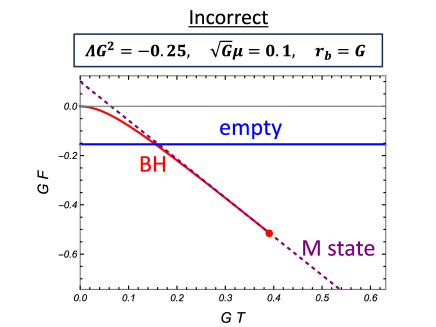
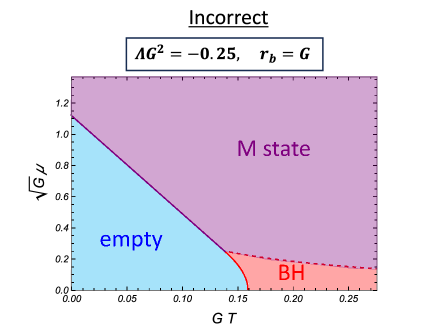
Figure 1: Incorrect $F-T$ diagram and phase diagram. (For the empty and BH phases, they are correct.) In [3], they claimed that there are two phase transitions; one is the Hawking-Page transition between the empty and BH phases, the other is a second order phase transition between the BH phase and the M state. The transition point is the same as the termination point of the BH branch and it is given by (2.23) and marked with the red dot in the left figure. (2.23) also represents the boundary between the BH phase and the M states in the right figure. The boundary between the empty phase and the M state is given by the relation $T=\frac{\sqrt{1-\Lambda r_{b}^{2}}}{2\pi r_{b}}-\frac{\mu}{\pi}\sqrt{-\Lambda G}$.

2.2 BR saddles, BG saddles, and thermodynamics

Instead of their two claims, I would like to claim that the following two are correct;
 
My claim

• When taking the $r_{H}\to r_{b}$ limit of the BH saddles, it corresponds to the Bertotti-Robinson(BR) saddles. Its entropy is $S=\frac{\pi r_{b}}{2G}$, its charge is $Q=\frac{r_{b}}{2}\sqrt{\frac{-\Lambda}{G}}$, and its energy is $E=\frac{\sqrt{-\Lambda}}{4G}r_{b}$.
  And its temperature $T$ and its chemical potential $\mu$ are NOT arbitrary values.

• There is a critical temperature, beyond which there are no BH saddles. Above this temperature, “bag of gold(BG)” saddles give the dominant contribution.

Firstly, let’s show the limit $r_{H}\to r_{b}$ does not corresponds to the situation where “the black hole merges with the cavity” but to the Bertotti-Robinson (BR) geometry. Define a small parameter $\varepsilon$ by $r_{H}=r_{b}-\varepsilon$. The first and second derivatives of $f(r)$ at $r=r_{H}=r_{b}-\varepsilon$ is

$$f^{\prime}(r_{H})=\frac{-\Lambda}{G\mu^{2}}(1-2G\mu^{2})\varepsilon+O(\varepsilon^{2})$$ (2.26)

$$f^{\prime\prime}(r_{H})=-4\Lambda+O(\varepsilon)\hskip 65.44142pt$$ (2.27)

By defining a new coordinate $r=r_{H}+\varepsilon\tilde{r},t=\frac{\tilde{t}}{\varepsilon}$, the metric becomes

$$\boldsymbol{g}=\left[\frac{-\Lambda}{G\mu^{2}}(1-2G\mu^{2})\tilde{r}-2\Lambda\tilde{r}^{2}+O(\varepsilon)\right]d\tilde{t}^{2}+\frac{1}{\left[\frac{-\Lambda}{G\mu^{2}}(1-2G\mu^{2})\tilde{r}-2\Lambda\tilde{r}^{2}+O(\varepsilon)\right]}d\tilde{r}^{2}+(r_{b}+O(\varepsilon))^{2}d\phi^{2}$$

(2.28)

Then, $\varepsilon\to 0$ limit (i.e. near horizon and near extremal limit) leads to

$$\boldsymbol{g}=\left[\frac{-\Lambda}{G\mu^{2}}(1-2G\mu^{2})\tilde{r}-2\Lambda\tilde{r}^{2}\right]d\tilde{t}^{2}+\frac{1}{\left[\frac{-\Lambda}{G\mu^{2}}(1-2G\mu^{2})\tilde{r}-2\Lambda\tilde{r}^{2}\right]}d\tilde{r}^{2}+r_{b}^{2}d\phi^{2}$$ (2.29)

$$\tilde{r}\in[0,1]$$ (2.30)

which is the Euclidean version of the 3-dimensional Bertotti-Robinson (BR) geometry. The gauge field can be obtained in a similar way, i.e,

$$\boldsymbol{A}=A_{t}(r)dt\hskip 71.13188pt$$

$$=\left[\sqrt{\frac{-\Lambda}{G}}\varepsilon\tilde{r}+O(\varepsilon^{2})\right]\frac{d\tilde{t}}{\varepsilon}$$

$$\to-i\sqrt{\frac{-\Lambda}{G}}\tilde{r}d\tilde{t}\hskip 45.52458pt$$ (2.31)

As with the standard argument for BHs, the absence of a conical singularity at $\tilde{r}=0$ leads to the unique temperature;

$$T_{BR}=\frac{\sqrt{-\Lambda}}{4\pi}\frac{1-2G\mu^{2}}{\sqrt{G}\mu}$$ (2.32)

which of course is the same as (2.23). We can also check that the parameter $\mu$ is actually the chemical potential of this saddle $\displaystyle\frac{A_{\tilde{t}}(\tilde{r}=1)}{\sqrt{g_{\tilde{t}\tilde{t}}}}=\mu$. Free energy and other thermodynamical quantities are given by

$${\rm\underline{free~{}energy}}\hskip 361.3499pt$$

$${\rm BR~{}saddle:}~{}~{}F=\frac{\sqrt{-\Lambda}}{4G}r_{b}-\frac{r_{b}}{8G\mu}\sqrt{\frac{-\Lambda}{G}}-\frac{r_{b}\mu}{4}\sqrt{\frac{-\Lambda}{G}}\hskip 142.26378pt$$ (2.33)

$${\rm\underline{thermodynamical~{}quantity}}\hskip 284.52756pt$$

$${\rm BR~{}saddle:}~{}~{}E=\frac{\sqrt{-\Lambda}}{4G}r_{b}\hskip 267.45572pt$$ (2.34)

$$S=\frac{\pi r_{b}}{2G}\hskip 285.95027pt$$ (2.35)

$$Q=\frac{r_{b}}{2}\sqrt{\frac{-\Lambda}{G}}\hskip 263.18799pt$$ (2.36)

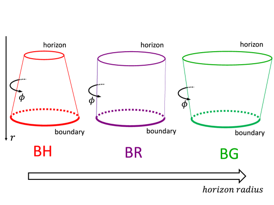
Figure 2: Spatial section of the BH saddle, BR saddle, and BG saddle. They are characterized by the radius of the horizon (or bolt); whether it is smaller or larger than the radius of the boundary.

So far, we have seen that the $r_{H}\to r_{b}$ limit of BH saddles is not a singular geometry of zero size but a BR saddle, whose circumference of the transverse circle remains constant in the radial direction. Since the limit is not singular, one might wonder whether a further deformation of saddles (i.e. the extension of the parameter range of $r_{H}$ beyond $r_{b}$ of BH saddles) is possible. In fact, it is possible. [1] (Fig. 2)

For the metric and gauge field (2.5), (2.6), we still have regular geometries when $r_{H}>r_{b}$. These are “bag of gold(BG)” saddles. The role of these saddles in pure gravity is discussed in [6, 7, 8] and their importance for the 4-dimensional Einstein-Maxwell system was recently shown in [1]. To distinguish it from the BH, let’s use $r_{G}$ for the horizon radius of BG saddles. The expression of boundary conditions, thermodynamical quantities, and free energy are all the same except for the following two points [1]; (i) Since $r$ is increasing toward the bolt, $f^{\prime}(r_{G})$ is negative. So there is a minus sign in the relation between $\beta$ and $f^{\prime}(r_{G})$ (2.37). (ii) Since the $r$ component of the normal vector of the boundary is negative for the same reason as before, $Q$ is not $\tilde{Q}$, but $Q=-\tilde{Q}$ (2.41). Summarize,

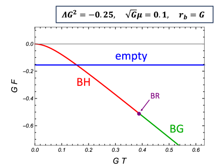
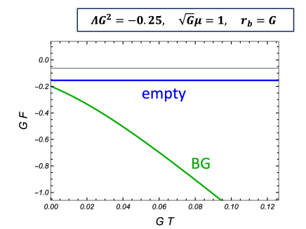
Figure 3: Behavior of the free energies. The terminal point of the BH branch corresponds to the BR saddle. Above the terminal temperature, there are BG phases which are thermodynamically stable. For low $\mu$, there is a Hawking-Page phase transition between BH/BG phases as shown in the left figure. For high $\mu$, the Hawking-Page phase transition does not occur and the system is in the BH/BG phase for all $T$ as in the right figure. The left figure is the correct version of Fig. 1.

$${\rm\underline{boundary~{}condition}}\hskip 318.67078pt$$

$${\rm BG~{}saddle:}~{}~{}\frac{-4\pi}{f^{\prime}(r_{G})}\sqrt{f(r_{b})}=\beta,~{}~{}\frac{2\tilde{Q}}{\sqrt{f(r_{b})}}\log\frac{r_{b}}{r_{G}}=\mu\hskip 83.93553pt$$ (2.37)

$${\rm\underline{free~{}energy}}\hskip 361.3499pt$$

$${\rm BG~{}saddle:}~{}~{}F=\frac{\sqrt{f(r_{b})}}{4G}+\frac{\sqrt{|\Lambda|}}{4G}r_{b}-\frac{\Lambda r_{G}^{2}}{4G\sqrt{f(r_{b})}}-\frac{\tilde{Q}^{2}}{\sqrt{f(r_{b})}}+\frac{2\tilde{Q}^{2}}{\sqrt{f(r_{b})}}\log\frac{r_{b}}{r_{G}}\hskip 8.5359pt$$ (2.38)

$${\rm\underline{thermodynamical~{}quantity}}\hskip 284.52756pt$$

$${\rm BG~{}saddle:}~{}~{}E=\frac{\sqrt{f(r_{b})}}{4G}+\frac{\sqrt{|\Lambda|}}{4G}r_{b}\hskip 204.85974pt$$ (2.39)

$$S=\frac{\pi r_{G}}{2G}\hskip 270.30118pt$$ (2.40)

$$Q=-\tilde{Q}\hskip 274.56891pt$$ (2.41)

The parameter range of $r_{G}$ is $r_{G}\in\left[r_{b},r_{b}e^{2G\mu^{2}}\right)$ and the $r_{G}\to r_{b}e^{2G\mu^{2}}$ limit corresponds to $T\to\infty$. Therefore, the BG branch is connected to the BH branch and is always present and is dominant above the BR temperature. The examples the free energy behavior are shown in Fig. 3. The behavior of the phase diagram depends on the value $-\Lambda r_{b}^{2}$ and are classified into three cases; the case of $0<-\Lambda r_{b}^{2}<1$, $-\Lambda r_{b}^{2}=-1$, and $1<-\Lambda r_{b}^{2}$. They are shown in Fig. 4.

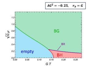
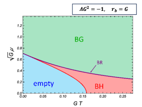
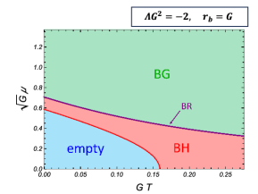
Figure 4: Examples of phase diagrams. The behavior of phase diagram depends on the value $-\Lambda r_{b}^{2}$ are classified into three cases; the case of $0<-\Lambda r_{b}^{2}<1$ (Left), $-\Lambda r_{b}^{2}=-1$ (Middle), and $1<-\Lambda r_{b}^{2}$ (Right). The left figure is the correct version of Fig. 1.

3 Difference between 3-dim. and 4-dim. ($\Lambda<0$)

There are many qualitative and quantitative differences between the Einstein-Maxwell system in 3-dimensions and that in 4-dimensions. What I want to emphasize here the most is the behavior of the BH phase (and the BG phase) in the phase diagram versus the value of $\Lambda$. In 4-dimensions, when we take $\Lambda\to 0$ limit or $\Lambda=0$, the phase diagram is still similar to the left figure in Fig. 4, i.e. there is a BH phase. However, in 3-dimensions, if we decrease the value of $-\Lambda r_{b}^{2}$, the BH phase shrinks. This can be seen from the fact that the boundary curve between the BH phase and the BG phase is given by (2.32) and the curve becomes close to the $T$ axis. This indicates that the BH phase disappear when $\Lambda=0$. The disappearance of the BH phase is not surprising, since, under some suitable conditions, including the dominant energy condition, it is proved that there are no BHs in 3-dimensions when $\Lambda=0$. [9, 10] Even for the system with a box boundary, this statement still be true. What may be surprising is the existence of the BG phase even for the $\Lambda\to 0$ limit. It seems to imply that even for $\Lambda=0$, the BG phase exists, possibly as a thermodynamically stable state. However, I will show in the next section that BG saddles do exist, but they cause thermodynamic instability.

4 $\Lambda=0$ case

In this case, there exist two types of saddles, the one is the empty saddle,

$$\boldsymbol{g}(r)=dt^{2}+dr^{2}+r^{2}d\phi^{2}$$ (4.1)

And the other saddle can be obtained by setting $\Lambda=0$ in (2.5), (and replacing the parameter $r_{H}$ with $r_{G}$,)

$$f(r)=-8GQ^{2}\log\frac{r}{r_{G}}$$ (4.2)

$$A_{t}(r)=2iQ\log\frac{r}{r_{G}}$$ (4.3)

Since for the coordinate range $r\in[r_{b},r_{G})$, $f(r)>0$ and $f(r_{G})=0$, this is the BG saddle, which is not singular. And here I also set $\tilde{Q}=-Q$ since these are BGs. The boundary conditions are similar to those in subsection 2.2. From the boundary conditions, we get the following expression;

$$\frac{1}{2G}\log\frac{r_{G}}{r_{b}}=\mu^{2}$$ (4.4)

$$T=\frac{Q}{2\pi r_{b}}\frac{1}{\mu e^{2G\mu^{2}}}$$ (4.5)

At this point, we know that, for fixed $\mu$, the entropy does not change no matter how we increase or decrease the temperature. This implies that the heat capacity is zero. Therefore, if these saddles give dominant contribution, it leads to thermodynamical instability of the system. Explicitly, free energy and thermodynamical quantities are given by

$${\rm\underline{free~{}energy}}\hskip 361.3499pt$$

$${\rm empty~{}saddle:}~{}~{}F=\frac{-1}{4G}\hskip 254.65207pt$$ (4.6)

$${\rm BG~{}saddle:}~{}~{}F=-\frac{Q^{2}}{\sqrt{f(r_{b})}}-\frac{2Q^{2}}{\sqrt{f(r_{b})}}\log\frac{r_{b}}{r_{G}}\hskip 142.26378pt$$

$$=-\frac{\pi r_{b}T}{2G}\left(1+4G\mu^{2}\right)e^{2G\mu^{2}}\hskip 153.6447pt$$ (4.7)

$${\rm\underline{thermodynamical~{}quantity}}\hskip 284.52756pt$$

$${\rm empty~{}saddle:}~{}~{}E=\frac{-1}{4G}\hskip 254.65207pt$$ (4.8)

$$S=0\hskip 266.03343pt$$ (4.9)

$$Q=0\hskip 266.03343pt$$ (4.10)

$${\rm BG~{}saddle:}~{}~{}E=0\hskip 267.45572pt$$ (4.11)

$$S=\frac{\pi r_{G}}{2G}=\frac{\pi r_{b}}{2G}e^{2G\mu^{2}}\hskip 193.47882pt$$ (4.12)

$$Q=2\pi r_{b}T\mu e^{2G\mu^{2}}\hskip 211.97293pt$$ (4.13)

Since, in this case, the BG free energy (4.7) is a linear function of $T$, the “transition temperature” can be easily found as

$$T_{tr}=\frac{1}{2\pi r_{b}\left(1+4G\mu^{2}\right)e^{2G\mu^{2}}}$$ (4.14)

The “phase diagram” is shown in Fig. 5.

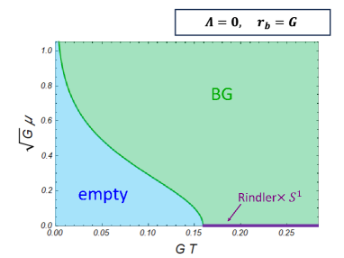
Figure 5: “Phase diagram” of the case where $\Lambda=0$. Since the BG “phase” is not thermodynamically stable, neither is the system itself.

Finally, let’s discuss what happens when we turn off $\mu$. From (4.4), we see that $\mu\to 0$ limit corresponds to $r_{G}\to r_{b}$ limit. Again, this limit does not lead to the merging of horizon and boundary but leads to a regular geometry, which is the direct product of the 2-dimensional Rindler space and $S^{1}$. By defining a small parameter $\varepsilon$ by $\varepsilon=G\mu^{2}$, the first derivative of $f$ at $r=r_{G}$ is

$$f^{\prime}(r_{G})=-\frac{8GQ^{2}}{r_{G}}=-32\pi^{2}r_{b}T^{2}\varepsilon+O(\varepsilon^{2})$$ (4.15)

Since $r_{G}=r_{b}e^{2\varepsilon}=r_{b}+2r_{b}\varepsilon+O(\varepsilon^{2})$, let’s define new coordinates by $(r_{G}-r)=2r_{b}\varepsilon\tilde{r},~{}t=\frac{\tilde{t}}{2r_{b}\varepsilon}$. Then, the ranges of these new coordinates will be $\tilde{r}\in[0,1],~{}\tilde{t}\in\left[0,\frac{1}{4\pi T^{2}}\right]$ in the $\varepsilon\to 0$ limit. Then, in the $\varepsilon\to 0$ limit, the metric and gauge field become

$$\boldsymbol{g}=\left[64\pi r_{b}^{2}T^{2}\varepsilon^{2}\tilde{r}+O(\varepsilon^{3})\right]\frac{d\tilde{t}^{2}}{4r_{b}^{2}\varepsilon^{2}}+\frac{4r_{b}^{2}\varepsilon^{2}}{\left[64\pi r_{b}^{2}T^{2}\varepsilon^{2}\tilde{r}+O(\varepsilon^{3})\right]}d\tilde{r}^{2}+(r_{b}+O(\varepsilon))^{2}d\phi^{2}$$

$$\to 16\pi^{2}T^{2}\tilde{r}d\tilde{t}^{2}+\frac{1}{16\pi^{2}T^{2}\tilde{r}}d\tilde{r}^{2}+r_{b}^{2}d\phi^{2}\hskip 184.9429pt$$ (4.16)

$$\boldsymbol{A}\to 0\hskip 345.7008pt$$ (4.17)

If we further define the coordinates $\rho$ and $\tau$ by $\tilde{r}=4\pi^{2}T^{2}\rho^{2},~{}\tau=8\pi^{2}T^{2}\tilde{t}$, the metric takes the standard Rindler form

$$\boldsymbol{g}=\rho^{2}d\tau^{2}+d\rho^{2}+r_{b}^{2}d\phi^{2}$$ (4.18)

$$\tau\in[0,2\pi],~{}\rho\in[0,2\pi T]$$ (4.19)

The free energy of the $Rindler\times S^{1}$ saddles is given by simply setting $\mu=0$ in the free energy of the BG saddles (4.7), and we can easily check that it will be dominant above the temperature $T=\frac{1}{2\pi r_{b}}$. (Fig. 5)

At first glance, the phase structures of the Einstein-Maxwell system in 3-dimensions and 4-dimensions are similar when $-\Lambda r_{b}^{2}$ is sufficiently large. There are three phases, the empty phase, the BH phase, and the BG phase (Fig. 4). However, when it is close to zero, differences appear; For 4-dimensions, the BH phase exists when $\Lambda\to 0$ or $\Lambda=0$, and the system is thermodynamically stable. For 3-dimensions, however, it shrinks in the $\Lambda\to 0$ limit and ceases to exist at $\Lambda=0$. So in 3-dimensions, when a negative $\Lambda$ is switched off, the boxed systems no longer have the saddles with the smaller horizon (i.e. BH saddles), as previously proved [9, 10], but still have the ones with the same size or larger horizon (i.e. BR saddles and BG saddles). But these saddles make the system thermodynamically unstable. When we also switch off $\mu$, the system does not allow the saddle with the larger horizon (BG saddle), but still allows the ones with the same size horizon (BR saddle, or $Rindler\times S^{1}$ saddle), which again makes the system thermodynamically unstable.

Appendix A Off-shell geometries for M states

This appendix is purely an appendix and has no direct relation to the result in this paper. In [3], they claimed that the $r_{H}\to r_{b}$ limit of the BH leads to the merging of the horizon and the boundary. Even for such non-geometrical states, they claimed that there are thermodynamical meaning and assigned the free energy of the form

$$F_{Mstate}(T,\mu)=\frac{\sqrt{-\Lambda}}{4G}r_{b}-T\frac{\pi r_{b}}{2G}-\mu\frac{r_{b}}{2}\sqrt{\frac{-\Lambda}{G}}$$ (A.1)

But in subsection 2.2, I showed that the limit corresponds to the BR geometry, which is a regular geometry and it does not have arbitrary temperature and chemical potential, but they have a relationship (2.32). Although the geometric picture of the M states was wrong, the free energy of the M states at the BR point was correct.

$$F_{Mstate}(T_{BR}(\mu),\mu)=F_{BR}(\mu)$$ (A.2)

In other words, at this BR point, the M state has a geometric picture, which is the on-shell BR geometry. So one might expect that other M states deformed from the M state at the BR point might have a geometric picture. Here, I show that BR geometries with a conical singularity

$$\boldsymbol{g}=\left[\frac{-\Lambda}{G\mu^{2}}(1-2G\mu^{2})\tilde{r}-2\Lambda\tilde{r}^{2}\right]d\tilde{t}+\frac{1}{\left[\frac{-\Lambda}{G\mu^{2}}(1-2G\mu^{2})\tilde{r}-2\Lambda\tilde{r}^{2}\right]}d\tilde{r}^{2}+r_{b}^{2}d\phi^{2}$$ (A.3)

$$\boldsymbol{A}=-i\sqrt{\frac{-\Lambda}{G}}\tilde{r}d\tilde{t}\hskip 277.41437pt$$ (A.4)

$$\tilde{r}\in[0,1],~{}~{}~{}~{}~{}~{}~{}\tilde{t}\in\left[0,\beta\mu\sqrt{\frac{G}{-\Lambda}}\right]\hskip 128.0374pt$$

can be a family of off-shell geometries whose free energy is given by (A.1). The parameters of this geometry are $r_{b},\mu$, and $\beta$, where $\beta$ is the circumference of the Euclidean time circle at the boundary. When $\displaystyle\beta\neq\beta_{BR}=\frac{4\pi}{\sqrt{-\Lambda}}\frac{\sqrt{G}\mu}{1-2G\mu^{2}}$, this geometry has a conical singularity at $\tilde{r}=0$, thus it is off-shell. The action functional for geometries with a conical singularity is given by [11]

$$I^{E}[\boldsymbol{g},\boldsymbol{A}]=\frac{-1}{16\pi G}\int_{\mathcal{M}\setminus\Sigma}d^{3}x\sqrt{g}(\mathcal{R}-2\Lambda)+\frac{1}{16\pi}\int_{\mathcal{M}\setminus\Sigma}d^{3}x\sqrt{g}F_{\mu\nu}F^{\mu\nu}\hskip 113.81102pt$$

$$+\frac{-1}{8\pi G}\int_{\partial\mathcal{M}}d^{2}y\sqrt{\gamma}\Theta+\frac{1}{8\pi G}\int_{\partial\mathcal{M}}d^{2}y\sqrt{\gamma}\sqrt{|\Lambda|}+\frac{-1}{8\pi G}\int_{\Sigma}d\phi\sqrt{\sigma}(2\pi-\theta(\phi))$$ (A.5)

The last term is for conical singularities and $\Sigma$ represents the codimension-two surface of a conical singularity and $2\pi-\theta(\phi)$ represents the (position dependent) conical deficit on the surface. The bulk and boundary terms are the same as for a regular BR, i.e. they are given by $\beta$ times $F_{BR}$ (2.33). The additional contribution comes from the last term. Substituting (A.3) for it gives

$$\frac{-1}{8\pi G}\int_{\Sigma}d\phi\sqrt{\sigma}(2\pi-\theta(\phi))=\frac{-r_{b}}{4G}\left(2\pi+\frac{\Lambda}{2G\mu^{2}}(1-2G\mu^{2})\beta\mu\sqrt{\frac{G}{-\Lambda}}\right)$$

$$=-\frac{\pi r_{b}}{2G}+\frac{r_{b}}{8G\mu}\sqrt{\frac{-\Lambda}{G}}\beta-\frac{r_{b}}{4}\sqrt{\frac{-\Lambda}{G}}\beta\mu\hskip 22.76228pt$$ (A.6)

Therefore, the “off-shell” free energy of these singular BR geometries is given by

$$F_{singularBR}=F_{BR}+T\times(\ref{FS})\hskip 248.96161pt$$

$$=\frac{\sqrt{-\Lambda}}{4G}r_{b}-\frac{r_{b}}{8G\mu}\sqrt{\frac{-\Lambda}{G}}-\frac{r_{b}\mu}{4}\sqrt{\frac{-\Lambda}{G}}-\frac{\pi r_{b}}{2G}T+\frac{r_{b}}{8G\mu}\sqrt{\frac{-\Lambda}{G}}-\frac{r_{b}}{4}\sqrt{\frac{-\Lambda}{G}}\mu$$

$$=\frac{\sqrt{-\Lambda}}{4G}r_{b}-\frac{\pi r_{b}}{2G}T-\frac{r_{b}}{2}\sqrt{\frac{-\Lambda}{G}}\mu\hskip 192.05609pt$$ (A.7)

which is equivalent to the free energy of the M state (A.1).

References

- [1] S. Miyashita , arXiv: 2402.16113
- [2] P. Basu, C. Krishnan, and P. N. B. Subramanian , JHEP (2016) 041
- [3] Y. Huang and J. Tao , Nucl. Phys. B (2022) 115881
- [4] J. D. Brown and J. W. York, Jr. , Phys. Rev. D (1993) 1407
- [5] T. V. Fernandes and J. P. S. Lemos , Phys. Rev. D108 (2023) 084053
- [6] S. Miyashita , JHEP (2021) 121
- [7] P. Draper and S. Farkas , Phys. Rev. D (2022) 126021
- [8] B. Banihashemi and T. Jacobson, JHEP (2022) 042
- [9] D. Ida, Phys. Rev. Lett. (2000) 3758
- [10] C. Krishnan, R. Shekhar, P. N. B. Subramanian , Nucl. Phys. B (2020) 115115
- [11] D. V. Fursaev and S. N. Solodukhin, Phys. Rev. D (1995) 2133