On Diffusion Process in SE(3)-invariant Space

Abstract

Sampling viable 3D structures (e.g., molecules and point clouds) with SE(3)-invariance using diffusion-based models proved promising in a variety of real-world applications, wherein SE(3)-invariant properties can be naturally characterized by the inter-point distance manifold. However, due to the non-trivial geometry, we still lack a comprehensive understanding of the diffusion mechanism within such SE(3)-invariant space. This study addresses this gap by mathematically delineating the diffusion mechanism under SE(3)-invariance, via zooming into the interaction behavior between coordinates and the inter-point distance manifold through the lens of differential geometry. Upon this analysis, we propose accurate and projection-free diffusion SDE and ODE accordingly. Such formulations enable enhancing the performance and the speed of generation pathways; meanwhile offering valuable insights into other systems incorporating SE(3)-invariance.

1 Introduction

Recently, there has been an increasing interest in utilizing diffusion-based generative models to sample 3-dimensional (3D) structures (Shi et al., 2021; Luo et al., 2021; Xu et al., 2022; Jing et al., 2022; Zhou et al., 2023; Fan et al., 2023a, b; Zhang et al., 2023). These approaches have demonstrated promising modeling ability in capturing the wide distribution of 3D coordinates, wherein the incorporation of the inherent roto-translational property of SE(3)-invariant space is considered as one of the key factors potentially leading to these successes (De Bortoli et al., 2022).

For 3D structures, the inter-node distance matrix is inherently equipped with SE(3)-invariance, thus being a natural and flexible choice for modeling the underlying diffusion process. To perform diffusion-based generation on this manifold, estimating the associated score function is essential (Song et al., 2020a). Unfortunately, the geometry over this manifold is highly irregular and non-trivial, yielding significant difficulty in mathematical and accurate estimation. While some recent works simplify the diffusion process with Gaussian (Xu et al., 2022) or Maxwell-Boltzmann (Zhou et al., 2023) assumptions, these heuristics may result in sub-optimal performance. Till now, extant literature has not systematically undertaken an in-depth analysis of the diffusion process in this manifold.

In parallel, some other trials seek to avoid direct manipulations on this manifold. Certain methodologies address the SE(3) group (Ganea et al., 2021), offering a means to overcome the SE(3)-invariance obstacle through prior knowledge. In the context of molecular conformation generation tasks, specific endeavors employ RDkit to initially generate local 3D structures, subsequently employing diffusion techniques to derive torsional angles (Jing et al., 2022). Alternatively, models geared towards protein generation delve into the SE(3) Lie group, capitalizing on the intrinsic dependency of protein properties on bond angles and lengths (Anand & Achim, 2022; Yim et al., 2023). However, the applicability of these modeling schemes is confined to specific tasks and proves inflexible to extend to generic 3D coordinate generation. In the case of point clouds, the majority of existing studies do not explicitly formulate designs for SE(3)-invariance (Zhou et al., 2021; Luo & Hu, 2021; Mo et al., 2023; Zeng et al., 2022). Instead, they commonly employ diffusion techniques directly on node embeddings. Notably, some achieve commendable performance by leveraging transformer architectures, anticipating the model to implicitly learn SE(3)-invariance in brute force.

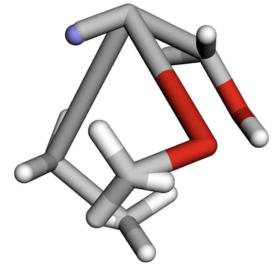
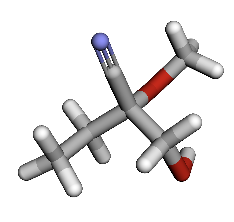
Figure 1: We utilized a sampling process with the off-the-shelf DPM-solver (Lu et al., 2022a) and our method in reduced sampling iterations (1000 steps) on a GeoDiff (Xu et al., 2022) model that was trained for 5000 steps. An example of a molecular conformer sampled via DPM-solver appears to be unreasonable (left), while our method produces a high-quality conformer (right).

The lack of a mathematical understanding of existing works raises additional concerns. Without accurate modeling, the reverse ODE and SDE formats of the diffusion process in SE(3)-invariant space remains opaque. Therefore, existing approximations usually sample 3D structures via naive Langevin dynamics (LD) with thousands of steps (Shi et al., 2021; Xu et al., 2022). Directly applying modern solvers (e.g., DPM solver and high-order solvers (Dormand & Prince, 1980; Lu et al., 2022a)) is problematic and will produce unmeaningful structures. See Fig. 1 for an example. Besides, a coarse diffusive framework on Riemannian manifold (De Bortoli et al., 2022) requires projection operation on each sampling step, failing to be effectively accelerated as well.

To better understand the diffusion process in SE(3)-invariant space and facilitate downstream tasks, in this paper, we systematically investigate the correlated diffusion process in this space from the perspective of differential geometry and projected differential equations. To this end, we mathematically derive the transformation between inter-point distance change and coordinate shift, delivering linear operations with bounded errors to mimic a projection into SE(3)-invariant space. As such, we propose projection-free SDE and ODE formulations to reverse the diffusion process. These findings offer useful insights into the mathematical mechanism of diffusion in SE(3)-invariant space. Extensive experiments are conducted on molecular conformation generation (Axelrod & Gomez-Bombarelli, 2022) and pose skeleton generation (Ionescu et al., 2013). Our scheme can sample high-quality 3D coordinates with only a few steps. In summary, our contributions are:

• We systematically investigate how to accurately model the diffusion-based generation in SE(3)-invariant space by considering the adjacency matrices for 3D coordinate generation tasks.

• We analyze the mappings between the SE(3)-invariant Cartesian space and matrix manifold and propose a linear operation to approximate the projection operation with bounded errors.

• We propose a novel projection-free sampling scheme by solving the reverse SDE and ODE via samplings between coordinates and adjacency matrices, allowing for simple acceleration.

2 Related works

Coordinate generation from SE(3)-invariant distribution.

Generating 3D coordinates of geometric structures (e.g., molecular conformation and point clouds) is a challenging task. In the context of molecular conformation or protein structure generation, some notable approaches focus on modeling the bound length and bound angles by considering the SE(3) group (Ganea et al., 2021; Jing et al., 2022; Yim et al., 2023; Anand & Achim, 2022). In contrast, DMCG (Zhu et al., 2022) presents an end-to-end solution by directly predicting atom coordinates while ensuring roto-translational invariance through an SE(3)-invariant loss function. More recently, there has been growing interest in modeling the inter-atomic distances, which naturally possess SE(3)-invariance. Certain approaches (Shi et al., 2021; Zhang et al., 2023; Luo et al., 2021; Xu et al., 2022; Zhou et al., 2023) introduce perturbations to the inter-atomic distances and subsequently estimate the corresponding coordinate scores. In the domain of point cloud generation, most works directly introduce noise to coordinates or latent features (Luo & Hu, 2021; Mo et al., 2023; Zeng et al., 2022), assuming that the learned point embeddings can implicitly incorporate SE(3) invariance (Wen et al., 2021; Zamorski et al., 2020; Wu et al., 2016).

Sampling acceleration of diffusion-based models.

Standard diffusion-based generation typically takes thousands of steps. To accelerate this, some new diffusion models such as consistency models (Song et al., 2023) are proposed. Consistency models directly map noise to data, enabling the generation of images in only a few steps. EC-Conf (Fan et al., 2023b) is an application of consistency models in substantially reduced steps for molecular conformation generation. Another straightforward approach is reducing the number of sampling iterations. DDIM (Song et al., 2020a) uses a hyper-parameter to control the sampling stochastical level and finds that decreasing the reverse iteration number improves sample quality due to less stochasticity. This phenomenon can be attributed to the existence of a probability ODE flow associated with the stochastic Markov chain of the reverse diffusion process (Song et al., 2020b), leading to the advent of numerical ODE solvers for acceleration. DPM-solver (Lu et al., 2022a) leverages the semi-linear structure of probability flow ODE to develop customized ODE solvers, and also provides high-order approximates for the probability ODE flow which can generate high-quality samples in only 10 to 20 iterations. Then DPM is extended to DPM-solver++ (Lu et al., 2022b) for sampling with classifier-free guidance. However, such a dedicated solver can only be applied in Euclidean space, and developing diffusion solvers for SE(3)-invariant space or on the pairwise distance manifold remains an open problem.

3 Preliminary

3.1 Euclidean diffusion and score matching objective

Given a random variable $\mathbf{x}_{0}\in\mathbb{R}^{n}$ following an unknown data distribution $q_{0}$, denoising diffusion probabilistic models (Song & Ermon, 2019; Ho et al., 2020; Song et al., 2020b) define a forward process $\{\mathbf{x}_{t}\}_{t\in[0,T]}$ following an Ito SDE

$$\mathrm{d}\mathbf{x}_{t}=f(t)\mathbf{x}_{t}\mathrm{d}t+g(t)\mathrm{d}\mathbf{w}_{t},\quad\mathbf{x}_{0}\sim q_{0},$$ (1)

where $\mathbf{w}_{t}\in\mathbb{R}^{n}$ is the standard Brownian motion and $f(t)$, $g(t)$ are chosen functions. Such a forward process has an equivalent reverse process starting from time $T$ to $0$:

$$\mathrm{d}\mathbf{x}_{t} =\left[f(t)\mathbf{x}_{t}-g^{2}(t)\nabla_{\mathbf{x}}\log q_{t}(\mathbf{x}_{t})\right]\mathrm{d}t+g(t)\mathrm{d}\mathbf{w}_{t},$$ (2)

where $\mathbf{x}_{T}\sim q_{T}(\mathbf{x}_{T}\mid\mathbf{x}_{0})\approx q_{T}(\mathbf{x}_{T})$, and the marginal probability densities $\{q_{t}(\mathbf{x}_{t})\}_{t=0}^{T}$ of the above SDE is the same as the following probability flow ODE (Song et al., 2020b):

$$\frac{\mathrm{d}\mathbf{x}_{t}}{\mathrm{d}t}=f(t)\mathbf{x}_{t}-\frac{1}{2}g^{2}(t)\nabla_{\mathbf{x}}\log q_{t}(\mathbf{x}_{t}).$$ (3)

This implies that if we can sample from $q_{T}(\mathbf{x}_{T})\approx q_{T}(\mathbf{x}_{T}\mid\mathbf{x}_{0})$ and solve Eq. (3), then the obtained $\mathbf{x}_{0}$ follows the distribution of $q_{0}(\mathbf{x}_{0})$. The only unknown terms in Eq. (3) are $q_{T}(\mathbf{x}_{T})$ and $\nabla_{\mathbf{x}}\log q_{t}(\mathbf{x}_{t})$. By choosing some specific $f(t)$ and $g(t)$, the distribution $q_{T}(\mathbf{x}_{T}\mid\mathbf{x}_{0})$ converges to $q_{T}(\mathbf{x}_{T})$ as $T\rightarrow\infty$ and $q_{T}$ is an easy distribution for sampling like Gaussian distribution. The score of the diffused data $\nabla_{\mathbf{x}}\log q_{t}(\mathbf{x}_{t})$ can be approximatively learned by a score-based model.

3.2 Diffusion on manifolds

In mathematical terms, a probability distribution $p(\mathbf{x})$ is considered invariant concerning the $\operatorname{SE}(3)$ group if $p(T(\mathbf{x}))=p(\mathbf{x})$ for any arbitrary transformations $T$ belonging to the $\operatorname{SE}(3)$ group. In terms of 3D coordinate generation following an SE(3)-invariant distribution, an effective and general strategy is to employ adjacency matrices or inter-atomic distances, which naturally exhibit invariance concerning the $\operatorname{SE}(3)$ groups (Gasteiger et al., 2020; Shi et al., 2021; Xu et al., 2022). An adjacency matrix $d=[d_{ij}]\in\mathbb{R}^{n\times n}_{+}$ is said to be feasible if there is a set of coordinates $\mathcal{C}=[\mathbf{x}_{1},\ldots,\mathbf{x}_{n}]^{\top}$ such that $d_{ij}=\|\mathbf{x}_{i}-\mathbf{x}_{j}\|,\forall i,j=1,\ldots,n$. Opposite to the usual diffusion on feature vectors laying in Euclidean space $\mathbb{R}^{n}$, feasible adjacency matrices only lay in a subset of the Euclidean space $\mathbb{R}^{n\times n}$. This subset is a manifold and we call this manifold the adjacency matrix manifold. If we directly perturb or add Gaussian noise to the adjacency matrix, we may obtain an infeasible adjacency matrix. To overcome such difficulty, we need to consider the context of diffusion on Riemannian manifolds (De Bortoli et al., 2022), which forces the diffusion objective to always lie in the specified manifolds. However, diffusion in manifolds often requires thousands of iterations and projection operations in each iteration, which hinders an effective sampling algorithm with fewer steps.

4 Method

In this work, we aim to explicitly compute the reverse SDE/ODE of SE(3)-invariant diffusion models. We consider SE(3)-invariant diffusion models equipped with pairwise distances and seek to develop a forward and reverse diffusion process on the adjacency matrix with the SE(3)-invariance. The overall mathematical scheme can be seen from Fig. 2.

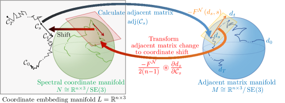
Figure 2: Mathematical framework for the reverse diffusion in the SE(3)-invariant space $\mathbb{R}^{n\times 3}/\operatorname{SE}(3)$. The grey rectangle denotes the coordinate embedding matrix manifold $L=\mathbb{R}^{n\times 3}$. The green ball denotes an SE(3)-invariant manifold $N$ of spectral coordinates (see Theorem 8) that is a submanifold of $L$. The blue ball denotes the adjacency matrix manifold $M$. Detailed definitions for the above three manifolds can be found in Appendix C.1. Each coordinate in the spectral coordinate manifold $N$ has a unique adjacency matrix in the adjacency matrix manifold $M$, and vice versa. During each step of the denoising process, given a noised sample $\mathcal{C}_{s}\in L$, our model predicts the change of the adjacency matrix $d_{s}=\operatorname{adj}\left(\mathcal{C}_{s}\right)$, illustrated by the orange tangent vector $-F^{\mathcal{N}}\left(d_{s},s\right)$ in the tangent space $T_{d_{s}}M$. Then we transform such a change of the adjacency matrix to the spectral coordinate shift by $\frac{-F^{\mathcal{N}}}{2(n-1)}\circledast\frac{\partial d_{s}}{\partial\mathcal{C}_{s}}$ (denoted by the red tangent vector in the tangent space of the spectral coordinate manifold). At the implementation level, we can further transform the tangent vector of spectral coordinates into the change of coordinates in the coordinate embedding space $L$ since this operation does not affect the values of the adjacency matrix.

4.1 Diffusion SDE of coordinates via adjacency matrices

Directly injecting noise on the adjacency matrix is inapplicable since this will violate the geometric properties of 3D structures (e.g., triangle inequality). Riemannian manifold diffusion (De Bortoli et al., 2022) addresses this issue by performing projection on each step but typically requiring thousands of steps. Besides, there is no literature on accelerating the Riemannian diffusion process. For the above two reasons, instead of directly working on the adjacency matrix manifold, we choose to inject noise on coordinates but consider modeling the corresponding evolving adjacency matrix, similar to Xu et al. (2022). Given a set of 3D coordinates $\mathcal{C}_{0}\in\mathbb{R}^{n\times 3}/\operatorname{SE}(3)$ and let $\mathcal{C}_{0}$ be represented or embedded by a $n\times 3$ matrix, i.e., $\mathcal{C}_{0}=[\mathbf{x}_{1},\ldots,\mathbf{x}_{n}]^{\top}\in\mathbb{R}^{n\times 3}$, we define a forward diffusion process of the coordinates embedding (we sometimes consider $\mathcal{C}_{0}$ as a vector to simplify our notations) (Song et al., 2020b)

$$\mathrm{d}\mathcal{C}_{t}=\mathbf{f}(\mathcal{C}_{t},t)\mathrm{d}t+\mathbf{G}(\mathcal{C}_{t},t)\mathrm{d}\mathbf{w}_{t},$$ (4)

where $\mathcal{C}_{0}\sim q_{0}(\mathcal{C}_{0})$ and $q_{0}$ is the distribution of the dataset, $t\in[0,T]$, $\mathbf{f}$ and $\mathbf{G}$ are two hyperparameters of noise scheduler and $\mathbf{w}_{t}\in\mathbb{R}^{n}$ is the standard Brownian motion. Let $p_{t}(\mathcal{C}_{t})$ be the distribution of $\mathcal{C}_{t}$. We use $\gamma_{1}(t)$ or $d_{t}$ to denote the corresponding adjacency matrix along with the diffusion process of the coordinates. Under some specific design of $\mathbf{f}$ and $\mathbf{G}$ (see Appendix C.5.2), the forward diffusion process of the adjacency matrix is given by

$$\mathrm{d}\gamma_{1}(t)=f(\gamma_{1}(t))\mathrm{d}t+g(t)\mathrm{d}\mathcal{B}_{t}^{M},$$ (5)

for some $f$ and $g$ which are dependent on $\mathbf{f}$ and $\mathbf{G}$, and $\mathcal{B}_{t}^{M}$ is the Brownian motion on the adjacen matrix manifold $M$. Eq. (5) is a diffusion process in the manifold of the adjacency matrix. At each time of the diffusion, $\gamma_{1}(t)$ is always a feasible adjacency matrix. If we discretize the reverse diffusion process of Eq. (5) in $N$ steps, then the reverse iterations are given by (De Bortoli et al., 2022)

$$d^{k-1}=\pi_{M,d^{k}}\left(d^{k}-F^{\mathcal{N}}(d^{k},kT/N)\right),$$ (6)

where

$$F^{\mathcal{N}}(d_{t},t) =\tau\left(f(d_{t})-g^{2}(t)\nabla_{d}\log p_{t}\left(d_{t}\right)\right)$$ (7)

$$\quad\quad+\sqrt{\tau}g(t)\mathbf{z}^{t,d_{t}},$$

where $\tau=T/N$, $\mathbf{z}^{t,d_{t}}$ is a standard normal random variable in the tangent space of $d_{t}$ and injected into $d_{t}$, and $\pi_{M,d^{k}}$ is the project operator whose output is a feasible adjacency matrix. $p_{t}(d_{t})=q_{t}(\mathcal{C}_{t})$ and $\nabla_{d}\log p_{t}\left(d_{t}\right)$ is the score function of the adjacency matrix which is hard to compute or approximate. Following Zhou et al. (2023), we assume that the distribution of distance change is a combination of Gaussian and Maxwell-Boltzmann distribution (see Eq. (21)). It is non-trivial to explicitly compute the formula for the projection operator $\pi_{M,d_{k}}$. We instead consider the corresponding reverse diffuion of the coordinates. Let $\varphi$ denote a smooth function that maps a feasible adjacency matrix to one of its coordinates. Such a mapping defines a manifold called the spectral coordinate manifold and we denote it as $N$. Note that each set of coordinates in the spectral coordinate manifold $N$ corresponds to a unique adjacency matrix and vice versa. Then we have

$$\mathcal{C}^{k-1}=\varphi\circ\pi_{M,d^{k}}\left(d^{k}-F^{\mathcal{N}}(d^{k},kT/N)\right)\in N.$$ (8)

To sample from the above iterations, we need to compute the formula for $\varphi\circ\pi_{M,d^{k}}$ which can be considered as a transformation from a non-necessary feasible adjacency matrix to a set of coordinates in manifold $N$. Finding the exact solution for $\varphi\circ\pi_{M,d^{k}}$ is also challenging. In the following, we will approximate the formula. Note that $\varphi\circ\pi_{M,d^{k}}$ is a function that maps a non-necessarily adjacency matrix to a set of coordinates whose adjacency matrix is closest to the function’s input. Let $\hat{d}=d^{k}+\sum_{i<j}\alpha_{ij}\bar{e}_{ij}$ and $\bar{e}_{ij}$ is a zero matrix except for entries $(i,j)$ and $(j,i)$ being 1. We can define $\varphi\circ\pi_{M,d^{k}}$ as an optimization problem as

Note that in the sampling process, we do not need to enforce the sampled coordinates in the spectral coordinate manifold $N$. Hence, we can ignore the constraint $\mathcal{C}\in N$ in the optimization problem at the implementation level. Hence, the optimization problem becomes

Compared with $d^{k}$, this adjacency matrix $\hat{d}$ has a small perturbation on each entry. We consider a simple case where $\hat{d}=d^{k}+\delta\bar{e}_{uv}$. We want to transform such a change of the adjacency matrix to the coordinate shift. We approximate that if the $(u,v)$ and $(v,u)$ entries of the adjacency matrix $d^{k}$ increase by $\delta$, then node $u$ and node $v$ go in their opposite directions by $\frac{\delta}{2(n-1)}$ where $n$ is the number of nodes. The term $n-1$ can be considered as the other $n-1$ nodes are rebelling against the extending of the edge $uv$. Such an approximation has a bounded error and does not explode as $n$ increases. For a more detailed analysis of such an approximation, we refer readers to Appendix C.3 and Appendix D and we summarize the error bound in the following theorem.

Theorem 1.

Consider the optimization problem $f(\hat{d})\triangleq\underset{\hat{\mathcal{C}}=[\hat{\mathbf{x}}_{1},\ldots,\hat{\mathbf{x}}_{M}]}{\min}\sum_{i<j}\left(\left\|\hat{\mathbf{x}}_{i}-\hat{\mathbf{x}}_{j}\right\|-\hat{d}_{ij}\right)^{2}$, where $\hat{d}=\tilde{d}+\delta\bar{e}_{uv}$. The optimal value $f(\hat{d})$ approximated by $\hat{\mathcal{C}}=\tilde{\mathcal{C}}+\frac{\delta}{2(n-1)}\frac{\partial\tilde{d}_{uv}}{\partial\tilde{\mathcal{C}}}$ where the adjacency matrix of $\tilde{\mathcal{C}}$ is $\tilde{d}$, is bounded by $\frac{2n^{2}-7n+6}{2(n-1)^{2}}\delta^{2}$.

We can extend the approximation results of simple case $\hat{d}=d^{k}+\delta\bar{e}_{uv}$ to the generic case $\hat{d}=d^{k}+\sum_{i<j}\alpha_{ij}\bar{e}_{ij}$ by the linearity of the differential (see Appendix C.3.3). Mathematically, we use $\simeq$ to denote the left and right-hand sides of the equation having the same adjacency matrix. Then Eq. (8) becomes

$$\mathcal{C}^{k-1}\simeq\mathcal{C}^{k}-\frac{F^{\mathcal{N}}(d^{k},kT/N)}{2(n-1)}\circledast\frac{\partial d^{k}}{\partial\mathcal{C}^{k}},$$ (11)

where $n$ is the number of nodes, $F^{\mathcal{N}}(d^{k},kT/N)\circledast\frac{\partial d^{k}}{\partial\mathcal{C}^{k}}=\frac{1}{2}\sum_{i,j=1,\ldots,n}F_{ij}^{\mathcal{N}}(d^{k},kT/N)\frac{\partial d_{ij}^{k}}{\partial\mathcal{C}^{k}}$. For the detailed mathematics derivation, we refer readers to Appendix C.1 to Appendix C.3. Although there may exist advanced but iterative algorithms for distance geometry (Moré & Wu, 1999; Chambolle & Pock, 2019) that may complex the gradient, we believe our simple but bounded approximated solution with linear operation can ease the gradient propagation in the training process and accelerate the sampling speed.

In Eq. (11), there are two unknown terms $f$ and $g$ in the function $F^{\mathcal{N}}$ depending on the choice of $\mathbf{f}$ and $\mathbf{G}$, which we want to eliminate as much as possible. By inspecting the discretization of forward SDE of coordinates and adjacency matrices, we find that Eq. (11) corresponds to the SDE

$$\mathrm{d}\mathcal{C}_{t} =\mathbf{G}(\mathcal{C}_{t},t)\mathrm{d}\mathbf{w}_{t}+\Bigl{(}\mathbf{f}(\mathcal{C}_{t},t)$$ (12)

$$\quad\quad-\frac{g^{2}(t)}{2(n-1)}\nabla_{d}\log p_{t}(d_{t})\circledast\frac{\partial d_{t}}{\partial\mathcal{C}_{t}}\Bigr{)}\mathrm{d}t.$$

A detailed derivation of Eq. (12) can be found in Appendix C.4.

Remark 2 (Necessity of alternating between coordinates and distances).

Alternating between spectral coordinates and distances within the analytical framework is imperative. This necessitates the conversion of coordinates to distances, wherein the model is deployed to equip with the SE(3)-invariance. Conversely, transitioning from distances to coordinates through $\varphi\circ\pi_{M}$ mimics the projection of a tangent vector onto the SE(3)-invariant manifold. Therefore, the interplay between these two distinct manifolds becomes indispensable for a comprehensive understanding of the underlying dynamics.

4.2 Reverse ODE of coordinates via adjacency matrices

Deriving the general reverse ODE for arbitrary forward diffusion on coordinates is challenging. In this paper, we only consider the variance exploding diffusion ($\mathbf{f}\equiv\mathbf{0}$) (Song & Ermon, 2019; Song et al., 2020b) and leave broader cases to our future work. To derive the reverse ODE, one may consider the Fokker-Planck equation for adjacency matrices. Given a set of coordinates $\mathcal{C}=[\mathcal{C}_{1},\ldots,\mathcal{C}_{n}]^{\top}\in\mathbb{R}^{n\times 3}$, we inject i.i.d. Gaussian noise to each node coordinate $\mathcal{C}_{i}$ and consider the change of distance between node $u$ and $v$. We found that if $\mathcal{C}_{i}^{t+\tau}=\mathcal{C}_{i}^{t}+\sqrt{\tau}\mathbf{z}_{i}^{t}$, $\mathbf{z}_{i}^{t}\sim\mathcal{N}(\mathbf{0},\sigma^{2}\mathbf{I})$, then $d_{uv}^{t+\tau}$ has the distribution of

$$d_{uv}^{t+\tau}=d_{uv}^{t}+\frac{2\sqrt{\tau}\mathbf{z}^{\top}(\mathcal{C}_{u}-\mathcal{C}_{v})+\tau\|\mathbf{z}\|^{2}}{\|\sqrt{\tau}\mathbf{z}+\mathcal{C}_{u}-\mathcal{C}_{v}\|+\|\mathcal{C}_{u}-\mathcal{C}_{v}\|},$$ (13)

where $\mathbf{z}\sim\mathcal{N}(\mathbf{0},2\sigma^{2}\mathbf{I})$. Utilizing the above equality, if $d_{uv}^{t+\tau}$ and $d_{uv}^{t}$ are obtained from Eq. (4) and Eq. (5), we have

$$\mathbb{E}\left[d_{uv}^{t}-d_{uv}^{t+\tau}\right]$$ (14a)

$$\qquad=\sqrt{\tau\pi}\mathbf{G}(t)L^{1/2}_{1/2}\left(\frac{-\|\mathcal{C}_{u}-\mathcal{C}_{v}\|^{2}}{2\sqrt{2\tau}\mathbf{G}(t)}\right)$$ (14b)

$$\qquad\approx-3\tau\mathbf{G}^{2}(t)/d_{uv}^{t}+\lito(\tau),$$ (14c)

$$\mathbb{E}\left[\left(d_{uv}^{t}-d_{uv}^{t+\tau}\right)^{2}\right]=2\tau\mathbf{G}^{2}(t)+\lito(\tau),$$ (14d)

where $L$ is the generalized Laguerre polynomial (Sonine, 1880). The above results play a pivotal role in formulating the reverse ODE of both adjacency matrices and coordinates. Unlike the diffusion process in Euclidean space, in the form of the expectation of the distance change, a term denoted as $d_{uv}^{t}$ emerges in the denominator. This implies that the magnitude of the distribution shift is contingent upon not only the selection of $\mathbf{G}(t)$ but also the present state of the adjacency matrix. We find that if we ignore the entry independence of the adjacency matrix and define the matrix division as an entry-wise matrix division, the reverse ODE of the adjacency matrix and coordinates are respectively

$$\mathrm{d}\gamma_{1}(t)=\left(3\frac{\mathbf{G}^{2}(t)}{\gamma_{1}(t)}-\mathbf{G}^{2}(t)\nabla_{\gamma_{1}}\log p_{t}\left(\gamma_{1}(t)\right)\right)\mathrm{d}t,$$ (15)

$$\frac{\mathrm{d}\mathcal{C}_{t}}{\mathrm{d}t}=\frac{\mathbf{G}^{2}(t)}{2\left(n-1\right)}\left(\frac{3}{d_{t}}-\nabla_{d}\log p_{t}\left(d_{t}\right)\right)\circledast\frac{\partial d_{t}}{\partial\mathcal{C}_{t}}.$$ (16)

A detailed analysis from Eq. (13) to Eq. (16) can be found in Appendix C.5.

4.3 Transformation for sparse graph

To sample from reverse diffusion, we need to train a model $\mathbf{s}_{\boldsymbol{\theta}}$ to predict $\nabla_{d}\log p_{t}\left(d_{t}\right)$. Note that for a graph with $n$ nodes, $\nabla_{d}\log p_{t}\left(d_{t}\right)$ is an $n$ by $n$ matrix and usually neural networks are designed for sparse graphs. Hence, we only consider predicting a portion of entries in the score function of distance. Note that for arbitrary graph topology, if the minimum edge degree is no less than 4, then the edge length set is bijection to its coordinate set under SE(3)-equivalence. In this case, analysis of mappings from the adjacency matrix change into the coordinate shift still holds and

where $N(i)$ denotes the neighborhood of node $i$ and $\operatorname{degree}_{i}$ represents the degree of node $i$. Under the methodology in Xu et al. (2022), we utilize a Message Passing Neural Network (MPNN) (Gilmer et al., 2017). The MPNN framework is employed to compute node embeddings $\boldsymbol{h}_{v}^{(t)}$ for all nodes $v\in V$ within the input graph $G$. This computation is performed through a series of $M$ layers of iterative message passing:

$$\boldsymbol{h}_{u}^{(m+1)}=\psi\left(\boldsymbol{h}_{u}^{(m)},\sum_{v\in N_{u}}\boldsymbol{h}_{v}^{(m)}\cdot\phi(\boldsymbol{e}_{uv},d_{uv})\right),$$ (18)

and the loss function is set to

$$\mathcal{L}\left(\boldsymbol{\theta};\left\{\sigma_{i}\right\}_{t=1}^{T}\right)\triangleq\frac{1}{T}\sum_{t=1}^{T}\frac{\sigma_{t}}{2}\mathbb{E}_{d_{0},d_{t}}\left[l\left(\boldsymbol{\theta},d_{t},d_{0}\right)\right],$$ (19)

$$l\left(\boldsymbol{\theta},d_{t},d_{0}\right)\triangleq\|\mathbf{s}_{\boldsymbol{\theta}}(d_{t},t)-\nabla_{d}\log p_{t}\left(d_{t}\mid d_{0}\right)\circledast\frac{\partial d_{t}}{\partial\mathcal{C}_{t}}\|_{2}^{2},$$ (20)

where $\mathbf{G}^{2}(t)=\frac{\mathrm{d}\sigma_{t}^{2}}{\mathrm{d}t}$. Following  Zhou et al. (2023), we assume the distribution of distance change follows

$$\nabla_{d}\log p_{t}\left(d_{t}\mid d_{0}\right)=\frac{a_{t}}{d_{t}}-\frac{d_{t}-d_{0}}{2\sigma_{t}^{2}},$$ (21)

where $a_{t}$ is a hyperparameter introduced to combine the Maxwell-Boltzemann and Gaussian distribution. When Eq. (19) is minimized, the obtained model $\mathbf{s}_{\boldsymbol{\theta}}(d_{t},t)\approx\nabla_{d}\log p_{t}(d_{t})\circledast\frac{\partial d_{t}}{\partial\mathcal{C}_{t}}$. However, since the pair-wise distances $d_{t}$ (a random variable) appear in the denominator, this may lead to an unstable training process. Inspecting the reverse ODE given by Eq. (16), we note that there is also a $d_{t}$ in the denominator. Hence, to eliminate the appearance of random variables in the denominator, we revise the score-matching objective to (which is also the hypothesis in Xu et al. (2022))

$$\nabla_{d}\log p_{t}\left(d_{t}\mid d_{0}\right)=-\frac{d_{t}-d_{0}}{2\sigma_{t}^{2}},$$ (22)

and we approximate the reverse ODE to be

$$\frac{\mathrm{d}\mathcal{C}_{t}}{\mathrm{d}t}=-\frac{\mathbf{G}^{2}(t)}{2\left(n-1\right)}\nabla_{d}\log p_{t}\left(d_{t}\right)\circledast\frac{\partial d_{t}}{\partial\mathcal{C}_{t}}.$$ (23)

4.4 Reverse process correction

In the proposed reverse diffusion process of both SDE and ODE, three approximations are made. Firstly, a linear operation is utilized to approximate the solution of the projection from the tangent space of the adjacency matrix to the manifold. Secondly, the dependence of the entries in the adjacency matrix is ignored. Thirdly, the score function of distance distribution is assumed to be the Gaussian one. To rectify these approximation errors, an additional value referred to as the “corrector” is introduced to the reverse SDE/ODE. The rationale behind this modification is that during the denoising process from $\mathcal{C}_{s}$ from $q_{s}\left(\mathcal{C}_{s}\right)$ to $q_{t}\left(\mathcal{C}_{t}\right)$, the obtained sample $\mathcal{C}_{t}$ after one step does not accurately align with the distribution of $q_{t}\left(\mathcal{C}_{t}\right)$ due to the presence of approximation errors. To mitigate these errors, it is desired to push $\mathbf{x}$ to take a larger step size. Therefore, the corrector is incorporated to amplify the step size. A more comprehensive analysis and discussion of this approach can be found in Appendix E.

Table 1: Comparison results between LD and our proposed SDE and ODE on QM9 and Drugs datasets under different sampling steps. Higher values for COV indicate that the model can generate samples with higher diversity. Lower values for MAT imply the model can generate high-quality samples with lower differences compared with the ground truth samples.

Datasets	Methods /# Steps	COV-R(%) $\uparrow$		MAT-R($\text{\,}\mathrm{\SIUnitSymbolAngstrom}$) $\downarrow$		COV-P(%) $\uparrow$		MAT-P($\text{\,}\mathrm{\SIUnitSymbolAngstrom}$) $\downarrow$
		Mean	Median	Mean	Median	Mean	Median	Mean	Median
QM9	LD   5000	90.07	93.39	0.2090	0.1988	52.79	50.29	0.4448	0.4267
	LD   100	88.07	90.20	0.2711	0.2808	54.80	52.42	0.5090	0.4552
	SDE 1000	89.25	94.02	0.2215	0.2180	55.15	52.42	0.4323	0.4164
	SDE 100	88.34	91.59	0.2763	0.2757	53.48	51.25	0.4870	0.4564
	ODE 1000	90.24	95.04	0.2052	0.1956	53.76	52.26	0.4304	0.4251
	ODE 100	90.81	96.56	0.2691	0.2765	48.73	47.16	0.5190	0.5026
Drugs	LD   5000	89.13	97.88	0.8629	0.8529	61.47	64.55	1.1712	1.1232
	LD   1000	82.92	96.29	0.9525	0.9334	48.27	46.03	1.3205	1.2724
	SDE 1000	83.39	91.02	0.9728	0.9784	58.43	60.28	1.2393	1.1814
	SDE 100	86.44	93.08	0.9261	0.9132	64.53	67.83	1.1584	1.1279
	ODE 1000	90.64	98.85	0.8493	0.8270	59.67	62.12	1.1915	1.1420
	ODE 100	87.76	98.59	0.9105	0.8846	53.32	54.27	1.8528	1.3563

5 Experiments

In this section, we empirically evaluate our proposed SDE (Eq. (12)) and ODE (Eq. (23)) for generating 3D coordinates, focusing on two tasks: molecular conformation generation and human pose generation. Initially, we outline the general baseline sampling methods, (annealed) Langevin dynamics (LD), followed by a detailed description of each task. Additional experimental settings and results are available in Appendix F.

5.1 Baseline

We compare our sampling approaches with the standard sampling method via LD (Song & Ermon, 2019):

$$\mathcal{C}_{t-1}=\mathcal{C}_{t}+\alpha_{t}\nabla_{\mathcal{C}}\log q_{t}(\mathcal{C}_{t})+\sqrt{2\alpha_{t}}\mathbf{z}_{t}^{\mathcal{C}_{t}},$$ (24)

for $t=N,\ldots,1$, where each entry of $\mathbf{z}_{t}^{\mathcal{C}_{t}}$ adheres to a standard normal distribution, $\alpha_{t}=\delta\sigma_{t}^{2}$ and $\delta$ signifies the hyper-parameter for step size that needs to be selected by grid search. In this section, we present the optimal results derived from experimenting with various step sizes, with comprehensive details on alternative step sizes available in Appendix F.2.2 and Appendix F.3.1. The term $\nabla_{\mathcal{C}}\log q_{t}(\mathcal{C}_{t})$ is approximated by $\nabla_{d}\log p_{t}\left(d_{t}\right)\circledast\frac{\partial d_{t}}{\partial\mathcal{C}_{t}}$, and an in-depth explanation can be found in Xu et al. (2022).

Modifying the step size $\delta$ allows for generation in fewer steps via LD, providing a conventional and equitable basis for comparison with our method. We assess both LD and our methods using the same trained model, trained over 5000 steps, with varied step counts in the sampling phase. Details on training and the backbone model are available in Appendix F.1.

5.2 Molecular conformation generation

Datasets.

We employ two datasets, namely GEOM-Drugs and GEOM-QM9 (Axelrod & Gomez-Bombarelli, 2022) to validate the performance of our sampling method. The dataset split is the same as Xu et al. (2020). The GEOM-QM9 test set contains 24,143 conformers originating from 200 molecules, averaging about 20 conformers per molecule. In the test set of the GEOM-Drugs dataset, we encounter 14,324 conformers from 200 molecules, with an average of approximately 47 atoms per molecule. In line with the previous work (Xu et al., 2020), we expand the generation of ground truth conformers to double their original quantity, resulting in more than 20k+ and 40k+ generated conformers.

Evaluation.

We adopt established evaluation metrics, namely Coverage (COV) and Matching (MAT), incorporating Recall (R) and Precision (P) aspects to assess the performance of sampling methods (Xu et al., 2020; Ganea et al., 2021). COV quantifies the proportion of ground truth conformers effectively matched by generated conformers, gauging diversity in the generated set. Meanwhile, MAT measures the disparity between ground truth and generated conformers, complementing quality assessment. Furthermore, refined metrics COV-R and MAT-R place added emphasis on the comprehensiveness of the ground truth coverage, while COV-P and MAT-P are employed to gauge the precision and accuracy of the generated conformers. More details can be found in Appendix F.2.1.

Comparison with LD method.

We compare the performance of our proposed SDE and ODE sampling methods against LD sampling across various steps, with the results detailed in Tab. 1. The evaluation encompasses eight metrics, and the displayed results are obtained under hyper-parameter settings that ensure a well-balanced comparison among these evaluation criteria. Additional results under varying hyperparameter conditions are available in Appendix F.2.2. Overall, our proposed methods can consistently achieve slightly better results than LD. These equivalent outcomes underscore the validity of our SDE and ODE sampling methods. In practice, the LD method’s path efficiency could be enhanced by modifying the step size. However, our SDE and ODE models are grounded in systematic mathematical reasoning within the SE(3)-invariant space, providing a robust theoretical basis. For qualitative analysis, Appendix F.2.3 showcases visualizations of the molecules generated by our SDE and ODE sampling methods. These results affirm that our approach efficiently and effectively produces meaningful 3D molecular geometries, thereby validating the effectiveness of our method.

5.3 Human pose generation

(a) LD
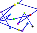
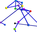
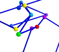
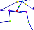
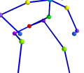
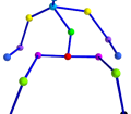
(b) Ours-SDE
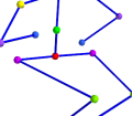
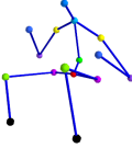
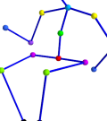
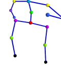
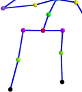
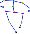
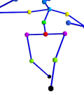
(c) Ours-ODE
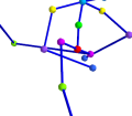
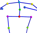
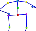
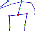
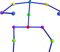
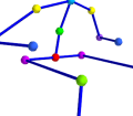
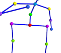
	steps=25	steps=50	steps=100	steps=250	steps=500	steps=1000	steps=2000

Figure 3: Visualization of sampling results obtained through LD and our proposed SDE/ODE with different sampling steps is presented. The human poses are labeled as “eating”. Samples are obtained from the exactly same trained model but drawn from different sampling algorithms. We grid search the hyperparameters in each sampling algorithm for a fair comparison.

Datasets and pre-processing.

We assess our sampling methods using the Human3.6M dataset (Ionescu et al., 2013), acknowledged as the most extensive dataset for human motion analysis. This dataset portrays seven actors engaged in 15 diverse actions, including walking, eating, discussions, sitting, and phoning. Actors are delineated by a skeletal structure comprising 32 joints, from which 17 key points are extracted to represent a human pose. Adhering to the standard train-test evaluation protocol for Human3.6M dataset (Iskakov et al., 2019; Kocabas et al., 2019), we employ subjects 1, 5, 6, 7, and 8 for training, while subjects 9 and 11 are utilized for validation, resulting in 312,188 and 109,867 poses for training and validation, respectively.

The human body can be conceptualized as a graph, with joints as nodes linked by edges symbolizing limbs. Each node is defined by its 3D coordinates. Our goal is to efficiently generate multiple plausible 3D human poses. We normalize the 3D coordinates and introduce “virtual edges” to achieve comprehensive graph connectivity. Additional details on these processes are elaborated in Appendix F.3.

Evaluation.

Since human behavior is composed of many human poses, it is difficult to judge a specific behavior only from a single action. However, our purpose is to compare the rapidity and effectiveness of our sampling method. Thus we design a metric to evaluate the quality of the generated single action. Drawing inspiration from the minimum matching distance (MMD) employed in the evaluation of point cloud generation tasks and evaluation metrics in molecular conformation generation, we devise a novel evaluation approach known as Alignment Minimum Matching Distance (AD). This method not only captures the distribution variance between the generated samples and the comprehensive reference dataset but also gauges the quality of the generated sample itself. The formula for AD is defined as

$$\operatorname{AD}\triangleq\frac{1}{|S_{g}|}\sum_{\mathcal{X}\in S_{g}}\min_{\mathcal{X}_{r}\in S_{r}}\|\operatorname{Align}(\mathcal{X},\mathcal{X}_{r})-\mathcal{X}_{r})\|^{2}_{F},$$ (25)

where $S_{g}$ and $S_{r}$ denote generated and reference human pose, respectively. $\|\cdot\|_{F}$ denotes the Frobenius norm. The function $\operatorname{Align}$ is defined to minimize the Frobenius norm of $T(\mathcal{X})-\mathcal{X}_{r}$ by translations and rotations.

Comparison with LD method.

We apply our SDE/ODE and LD methods to generate 500 human poses labeled as eating, varying the steps from 25 to 2000. The quantitative results are presented in Table 2, highlighting the best outcomes for each method under optimal hyper-parameter settings. For comprehensive details on hyperparameters and varied results, refer to Appendix F.3.1. We found that our proposed SDE/ODE achieves much better results with a substantially reduced number of iterations compared with LD. The effectiveness of LD diminishes significantly as the number of steps decreases, whereas our methods maintain performance consistency across varying step counts. Qualitative comparisons in Fig. 3 reveal that while LD requires hundreds of steps to produce reasonable samples, our SDE/ODE method accomplishes this with far fewer steps. Additional samples are visualized in Appendix F.3.2. The outcomes of the human pose generation task suggest that our method, anchored in comprehensive theoretical derivation within the SE(3)-invariant manifold, potentially demonstrates enhanced versatility and applicability.

Table 2: Comparision of mean AD scores of the three sampling methods under 100, 250, 500, and 1000 steps, where a lower AD value indicates better performance.

	LD	SDE	ODE
100	5.1739	2.3737	2.8978
250	4.3071	2.3452	2.5739
500	4.0020	2.3463	2.2811
1000	3.7369	2.3315	2.1620

6 Conclusion

This paper elucidates the complex diffusion processes in SE(3)-invariant spaces by examining the interaction between coordinates and adjacency matrix manifolds. We introduce noise to coordinates in the forward process and use differential geometry for reverse process analysis, focusing on inter-point distance changes. This leads to projection-free SDE and ODE sampling methods, improving efficiency as well as interpretability. Our empirical tests in molecular conformation and human pose generation confirm the high efficiency and quality of our 3D coordinate generation methods. This work offers significant insights into SE(3)-invariant manifolds and broad applicability in 3D coordinate generation tasks.

Broader impact

This paper presents work whose goal is to advance the field of Machine Learning. There are many potential societal consequences of our work, none which we feel must be specifically highlighted here.

Appendix A Definition

Definition 3.

We define $\operatorname{adj}:\mathbb{R}^{n\times 3}\rightarrow\mathbb{R}_{+}^{n\times n}$ as the mapping from a set of coordinates of $n$ nodes to its adjacency matrix. Suppose $\mathcal{C}=[\mathbf{x}_{1},\ldots,\mathbf{x}_{n}]$, then

$$\operatorname{adj}_{ij}(\mathcal{C})=\|\mathbf{x}_{i}-\mathbf{x}_{j}\|,\quad\forall i,j=1,\ldots,n.$$ (26)

Definition 4.

We say an adjacency matrix $A\in\mathbb{R}^{n\times n}$ is feasible if there exists a set of non-planar $n$ coordinates $\mathcal{C}$ such that $\operatorname{adj}\left(\mathcal{C}\right)=A$. Non-planar coordinates have exactly 3 positive eigenvalues (see Theorem 8). If coordinates are planar (but not in a line), they only have two positive eigenvalues.

Definition 5.

In this paper, the matrix norm $\|\cdot\|$ is defined to be the Frobenius norm, i.e, given $A\in\mathbb{R}^{m\times n}$, $\|A\|=\|A\|_{\mathrm{F}}=\sqrt{\sum_{i=1}^{m}\sum_{j=1}^{n}a_{\mathrm{ij}}^{2}}$.

Definition 6.

We define the weighted product of matrix $A\in\mathbb{R}^{n\times n}$ and matrix $B\in\mathbb{R}^{n\times n\times s\times t}$ as

$$A\circledast B=\frac{1}{2}\sum_{i,j=1,\ldots,n}A_{ij}B_{ij},$$ (27)

where $A_{ij}\in\mathbb{R},B_{ij}\in\mathbb{R}^{s\times t}$ and $A\circledast B\in\mathbb{R}^{s\times t}$.

Definition 7.

Given two set of coordinates $\mathcal{C}_{1}$ and $\mathcal{C}_{2}$, if $\operatorname{adj}\left(\mathcal{C}_{1}\right)=\operatorname{adj}\left(\mathcal{C}_{2}\right)$, we write $\mathcal{C}_{1}\simeq\mathcal{C}_{2}$. Moreover, if two equations give the same marginal distribution density with respect to $q$ where $q$ is any SE(3)-invariant distribution density function, we refer such a marginal distribution identity as $\simeq$.

Appendix B Backgrounds

B.1 Introduction of differential geometry

Figure 4: Mappings between two manifolds.

In differential geometry, we consider mappings between two manifolds. Suppose that $\varphi:M\rightarrow N$ is a smooth map between smooth manifolds.

Tangent space $TM$.

In the following, we give an informal definition of the tangent space. The tangent space of manifold $M$ at $x\in M$, denoted by $T_{x}M$, is defined as the set of all tangent vectors $\gamma^{{}^{\prime}}(0)$ at $x$, where $\gamma$ is an arbitrary curve in the manifold $M$ satisfying $\gamma(t):(-1,1)\rightarrow M$ and $\gamma(0)=x$.

Tangent space projection $\pi_{M}$.

$\pi_{M}:TM\rightarrow M$ is the projection operator that maps a vector in the tangent space back to the manifold. The tangent space projection of $\hat{x}\in T_{x}M$ is defined by $\pi_{M,x}(\hat{x})=\operatorname{argmin}_{y\in M}\|y-\hat{x}\|$ for some norm $\|\cdot\|$. That is, we find the point $y$ in the manifold $M$ that is closest to $\hat{x}$.

Differential $\mathrm{d}\varphi$.

The differential of $\varphi$ at a point $x\in M$, denoted as $\mathrm{d}\varphi_{x}$ is the best linear approximation of $\varphi$ near $x$. The differential is analogous to the total derivative in calculus. Mathematically speaking, the differential $\mathrm{d}\varphi$ is a linear mapping from the tangent space of $M$ at $x$ to the tangent space of $N$ at $\varphi(x)$, which is $\mathrm{d}\varphi_{x}:T_{x}M\rightarrow T_{\varphi(x)}N$. Given an equivalence class of curves $\gamma:(-1,1)\rightarrow M$ where $\gamma(0)=x$, we have $\mathrm{d}\varphi_{x}\left(\gamma^{\prime}(0)\right)=(\varphi\circ\gamma)^{\prime}(0)$. Note that the linearity of the differential will be used in Eq. (46).

B.2 Introduction of spectral theorem

One of the primary challenges encountered in the analysis of the adjacency matrix lies in the dependencies that exist between certain entries. When a subset of the entries in the adjacency matrix is accessible, it becomes possible to infer the values of other unknown entries. The spectral theorem offers insights into transforming the adjacency matrices into alternative representations, thus enabling the elimination of redundant entries. This transformation process greatly simplifies the study of the relationship between coordinates and adjacency matrices. The subsequent theorem provides a guideline for identifying a set of coordinates that corresponds to a given adjacency matrix.

Theorem 8 (Adjacency matrix spectrum decomposition (Schoenberg, 1935; Gower, 1982; Hoffmann & Noé, 2019)).

For any feasible adjacency matrix $D\in\mathbb{R}_{+}^{n\times n}$ (Def. 4), there corresponds to a Gram matrix $M\in\mathbb{R}^{n\times n}$ by

$$M_{ij}=\frac{1}{2}(D_{1j}+D_{i1}-D_{ij})$$ (28)

and vice versa

$$D_{ij}=M_{ii}+M_{jj}-2M_{ij}.$$ (29)

Applying the singular value decomposition (SVD) to the Gram matrix $M\in\mathbb{R}^{n\times n}$ (associated with $D$), we can obtain exactly 3 positive eigenvalues $\lambda_{1},\lambda_{2},\lambda_{3}$ and their corresponding eigenvectors $\mathbf{v}_{1},\mathbf{v}_{2},\mathbf{v}_{3}$ satisfying $\lambda_{1}\geq\lambda_{2}\geq\lambda_{3}>0$. Then the set of coordinates

$$\mathcal{C}=[\mathbf{v}_{1},\mathbf{v}_{2},\mathbf{v}_{3}]\left[\begin{array}[]{lll}\@add@centering\centering\sqrt{\lambda_{1}}&\;\;\;0&\;\;\;0\\ \;\;\;0&\sqrt{\lambda_{2}}&\;\;\;0\\ \;\;\;0&\;\;\;0&\sqrt{\lambda_{3}}\end{array}\right]$$ (30)

satisfies $\operatorname{adj}\left(\mathcal{C}\right)=D$. We denote such a mapping from a feasible adjacency matrix $D$ to a set of coordinates as $\varphi:\mathbb{R}^{n\times n}_{+}\rightarrow\mathbb{R}^{n\times 3}$.

B.3 Introduction of Riemann manifold diffusion

Let $M$ denote a complete, orientable connected, and boundaryless Riemannian manifold, endowed with a Riemannian metric. Let $\mathcal{B}^{M}_{t}$ be a Brownian motion on $M$. Under some regularity conditions, given a forward diffusion process by $\mathrm{d}X_{t}=f(X_{t})\mathrm{d}t+g(t)\mathrm{d}\mathcal{B}_{t}^{M}$, where $X_{t}$ always stays in the manifold $M$, the reverse process of $X_{t}$ is associated with the SDE

$$\mathrm{d}X_{t}=\left(f(X_{t})-g^{2}(t)\nabla_{X}\log p_{t}\left(X_{t}\right)\right)\mathrm{d}t+g(t)\mathrm{d}\mathcal{B}_{t}^{M}.$$ (31)

This reverse process can be discretized into $N$ steps by

$$X^{k-1}=\pi_{M,X^{k}}\left(X^{k}+\tau\left(-f(X^{k})+g^{2}(kT/N)\nabla_{X}\log p_{kT/N}\left(X^{k}\right)\right)+\sqrt{\tau}g(kT/N)\mathbf{z}^{k}\right),$$ (32)

where $\mathbf{z}^{k}$ is a standard normal random variable in the tangent space of $T_{X^{k}}M$, and $\tau=T/N,k=N,\ldots,1$ (De Bortoli et al., 2022).

Appendix C Diffusion in manifolds

C.1 Manifolds related with SE(3)-invariant space

In the sampling process, the reverse diffusion trajectory in the embedding matrix manifold $L=\mathbb{R}^{n\times 3}$ is associated with a trajectory in the adjacency matrix manifold $M$. We can model the denoising trajectory in the adjacency matrix manifold to avoid considering the SE(3)-invariant property and then transform this adjacency matrix trajectory back to the embedding matrix manifold $L$. However, since the dimension of the adjacency manifold $M$ is smaller than that of the embedding manifold $L$, we cannot define a one-to-one mapping between $M$ and $L$. Instead, we consider a sub-manifold of the embedding manifold $L$, denoted by $N$ which shrinks the manifold dimension by removing the equivalent element w.r.t. translations and rotations. We want to construct a manifold $N$ containing a part of coordinate embeddings such that $M\cong N$ and $N\subset\mathbb{R}^{n\times 3}$. In the following, we give the detailed definitions of the above manifolds.

Embedding matrix manifold $L$.

We usually represent the coordinates of $n$ nodes by a matrix $\mathcal{C}\in\mathbb{R}^{n\times 3}$. All these representations form an embedding manifold $L$ and $L=\mathbb{R}^{n\times 3}$.

Adjacency matrix manifold $M$.

$M$ is the manifold of the feasible adjacency matrix (Def. 4). Since the pairwise distances are invariant under rotations and translations, transforming the diffusion process in the embedding manifold $L$ to the manifold $M$ can avoid the difficulty in considering the SE(3)-invariance.

Spectral coordinate manifold $N$.

We define the spectral coordinate manifold by $N=\{\varphi(d)\mid d\in M\}$. Since the $\varphi$ is a smooth mapping, the above-defined set is smooth. The intuition behind such a definition is that each element in $N$ is an equivalence class for all coordinates having the same adjacency matrix.

C.2 Manifold geometries

We consider mappings between manifolds so that we can transform the diffusion process in the embedding manifold $L$ to the adjacency matrix manifold $M$ or the spectral coordinate manifold $N$ to equip with the SE(3)-invariance. Consider a forward diffusion process on coordinates by

$$\mathrm{d}\mathcal{C}_{t}=\mathbf{f}(\mathcal{C}_{t},t)\mathrm{d}t+\mathbf{G}(\mathcal{C}_{t},t)\mathrm{d}\mathbf{w},$$ (33)

when we take some special forms of functions $\mathbf{f}$ and $\mathbf{G}$ (see Appendix C.5.2), we write the corresponding evolving adjacency matrix $\gamma_{1}\in\mathbb{R}_{+}^{n\times n}$ by:

$$\mathrm{d}\gamma_{1}(t)=f(\gamma_{1}(t))\mathrm{d}t+g(t)\mathrm{d}\mathcal{B}_{t}^{M}.$$ (34)

By the Riemann diffusion process (De Bortoli et al., 2022), the corresponding time-reverse diffusion SDE of $\gamma_{1}$ is given by

$$\mathrm{d}\gamma_{1}(t)=\left(f(\gamma_{1}(t))-g^{2}(t)\nabla_{\gamma_{1}}\log p_{t}\left(\gamma_{1}(t)\right)\right)\mathrm{d}t+g(t)\mathrm{d}\mathcal{B}_{t}^{M}.$$ (35)

Let

$$F^{\mathcal{N}}(\gamma_{1}(t),t)=\tau\left(f(\gamma_{1}(t))-g^{2}(t)\nabla_{\gamma_{1}}\log p_{t}\left(\gamma_{1}(t)\right)\right)+\sqrt{\tau}g(t)\mathbf{z}^{t,\gamma_{1}(t)},$$ (36)

where $\tau=T/N$ and $\mathbf{z}^{t,\gamma_{1}(t)}$ is a standard normal random variable in the tangent space of $T_{\gamma_{1}(t)}M$ which acts as the noise injected into $\gamma_{1}(t)$. Then Eq. (35) is discretized by

$$\gamma_{1}^{k-1}=\pi_{M,\gamma_{1}^{k}}\left(\gamma_{1}^{k}-F^{\mathcal{N}}(\gamma_{1}^{k},kT/N)\right),\quad k=N,\ldots,1.$$ (37)

There is an associated curve $\gamma_{2}(t)=\varphi\circ\gamma_{1}(t)$ in the spectral coordinate manifold $N$ (by Theorem 8) and the discretized trajectory can be computed by

$$\gamma_{2}^{k-1}=\varphi\left(\gamma_{1}^{k-1}\right)=\varphi\circ\pi_{M,\gamma_{1}^{k}}\left(\gamma_{1}^{k}-F^{\mathcal{N}}(\gamma_{1}^{k},kT/N)\right),\quad k=N,\ldots,1.$$ (38)

Since $N$ is a submanifold of $L$, if we can solve the denoising process by Eq. (38), then at the end of the denoising process (at $\gamma_{2}(0)$), the obtained sample follows the distribution of $p_{0}$. To solve Eq. (38), we must analyze two functions $\varphi\circ\pi_{M}(\cdot)$ and $F(\cdot)$. In the following, we will approximate them respectively.

C.3 Approximation of $\varphi\circ\pi_{M}$

In this section, we use $\tilde{d}$ to denote a feasible adjacency matrix in the denoising trajectory and we use $\hat{d}$ to denote a vector in the tangent space $T_{\tilde{d}}M$. We will use $\hat{\mathcal{C}}\in N$ to denote a set of coordinates whose adjacency matrix is close to $\hat{d}$, i.e. the solution of $\hat{C}=\varphi\circ\pi_{M,\tilde{d}}(\hat{d})$. Given $\hat{d}=\tilde{d}+\sum_{i<j}\alpha_{ij}\bar{e}_{ij}\in T_{\tilde{d}}M$, where $\bar{e}_{ij}$ is a zero matrix except for entries $(i,j)$ and $(j,i)$ being 1, our goal is to compute the value of $\varphi\circ\pi_{M,\tilde{d}}(\hat{d})$.

C.3.1 Definition of $\varphi\circ\pi_{M}$

$\varphi\circ\pi_{M}$ is the mapping from $T_{\tilde{d}}M$ to $N$. In other words, given a non-necessarily feasible adjacency matrix $\hat{d}\in T_{\tilde{d}}M$, we want to find an element $\hat{\mathcal{C}}\in N$ such that $\|\operatorname{adj}(\hat{\mathcal{C}})-\hat{d}\|\leq\|\operatorname{adj}(\mathcal{C})-\hat{d}\|$ for all $\mathcal{C}\in N$. We write $\hat{d}$ in the form of $\displaystyle\hat{d}=\tilde{d}+\sum_{i<j}\alpha_{ij}\bar{e}_{ij}\in T_{\tilde{d}}M$, where $\bar{e}_{ij}$ is a zero matrix except for entries $(i,j)$ and $(j,i)$ being 1. $\tilde{d}\in M$ and $\tilde{d}$ is a feasible adjacency matrix. Define $\pi_{M,\tilde{d}}(\hat{d})_{ij}\triangleq\left\|\hat{\mathbf{x}}_{i}-\hat{\mathbf{x}}_{j}\right\|$, where $\displaystyle\hat{\mathbf{x}}_{1},\ldots,\hat{\mathbf{x}}_{n}=\underset{\mathbf{x}_{1},\ldots,\mathbf{x}_{n}}{\operatorname{argmin}}\sum_{i<j}\left(\left\|\mathbf{x}_{i}-\mathbf{x}_{j}\right\|-\hat{d}_{ij}\right)^{2}.$ Composed with $\varphi:M\rightarrow N$, we add the constraint $\mathcal{C}=[\mathbf{x}_{1},\ldots,\mathbf{x}_{n}]\in N$ to the optimization problem and change the return values from the adjacency matrix to its associated coordinates $\mathcal{C}$ in the $N$ manifold. We have

$$\varphi\circ\pi_{M,\tilde{d}}(\hat{d})=\varphi\circ\pi_{M,\tilde{d}}(\tilde{d}+\sum_{i<j}\alpha_{ij}\bar{e}_{ij})=\underset{[\mathbf{x}_{1},\ldots,\mathbf{x}_{n}]\in N}{\operatorname{argmin}}\sum_{i<j}\left(\left\|\mathbf{x}_{i}-\mathbf{x}_{j}\right\|-\hat{d}_{ij}\right)^{2},\quad\hat{d}\in T_{\tilde{d}}M,\tilde{d}\in M.$$ (39)

In the reverse diffusion process, at $\tilde{d}=d_{t}$, our model takes the noised sample $\tilde{d}$ and predicts $\hat{d}\in T_{\tilde{d}}M$. Mathematically speaking, $T_{\tilde{d}}M$ has the same dimension as the $M$ manifold, which is less than $n^{2}$. However, we do not add any constraints on the model’s output. The predicted $\hat{d}$ may not lay in $T_{\tilde{d}}M$. To consider the above cases, we consider a more general optimization problem by expanding the domain of $\hat{d}$ into $\mathbb{S}^{n}$ (all symmetric matrices). That is, given $\displaystyle\hat{d}=\tilde{d}+\sum_{i<j}\alpha_{ij}\bar{e}_{ij}$ for some $\alpha_{ij}$, we define

$$\varphi\circ\pi_{M,\tilde{d}}(\hat{d})=\varphi\circ\pi_{M,\tilde{d}}(\tilde{d}+\sum_{i<j}\alpha_{ij}\bar{e}_{ij})=\underset{[\mathbf{x}_{1},\ldots,\mathbf{x}_{n}]\in N}{\operatorname{argmin}}\sum_{i<j}\left(\left\|\mathbf{x}_{i}-\mathbf{x}_{j}\right\|-\hat{d}_{ij}\right)^{2},\quad\hat{d}\in\mathbb{R}^{n\times n},\tilde{d}\in M.$$ (40)

In the following, we will investigate how to solve the above equation by first considering a simple case of $\hat{d}$ where $\hat{d}=\tilde{d}+\delta\bar{e}_{uv}$ for some $u,v=1,\ldots,n$ and then considering the generic case of $\hat{d}$ where $\displaystyle\hat{d}=\tilde{d}+\sum_{i<j}\alpha_{ij}\bar{e}_{ij}$.

C.3.2 Simple case of $\varphi\circ\pi_{M}$

Instead of directly computing $\displaystyle\varphi\circ\pi_{M,\tilde{d}}(\tilde{d}+\sum_{i<j}\alpha_{ij}\bar{e}_{ij})$, we first consider a simple case where $\hat{d}=\tilde{d}+\delta\bar{e}_{uv}$ and $\delta>0$. That is, compared with the generic cases where $\displaystyle\hat{d}=\tilde{d}+\sum_{i<j}\alpha_{ij}\bar{e}_{ij}$, we assume that only one among $\{\alpha_{ij}\}_{i,j=1,\ldots,n,i<j}$ is non-zero. Computing $\displaystyle\varphi\circ\pi_{M,\tilde{d}}(\tilde{d}+\delta\bar{e}_{uv})$ is exactly the same as finding a set of coordinates $\mathcal{C}\in\mathbb{R}^{n\times 3}$ such that $\|\hat{d}-\operatorname{adj}\left(\mathcal{C}\right)\|$ is minimized. Note that $\tilde{d}$ is associated with a set of coordinates $\tilde{\mathcal{C}}=[\tilde{\mathbf{x}}_{1},\ldots,\tilde{\mathbf{x}}_{n}]^{\top}\in N$. If we take $\mathcal{C}=\tilde{\mathcal{C}}$, then the matrix $\hat{d}-\operatorname{adj}\left(\mathcal{C}\right)$ has all 0 entries except entries $(u,v)$ and $(v,u)$ and these entries have the value $\delta$. We want to reduce the value of these entries so that the value of $\|\hat{d}-\operatorname{adj}(\mathcal{C})\|$ would reduce. To achieve this, we need to expand the edge length between node $u$ and $v$. A straightforward implementation is that we push node $u$ and $v$ in their opposite directions for some distance $s>0$ and other nodes maintain in their positions. That is if we denote the obtained new coordinates by $\hat{\mathcal{C}}=[\hat{\mathbf{x}}_{1},\ldots,\hat{\mathbf{x}}_{n}]^{\top}$, then we have

$$\left\{\begin{aligned} \hat{\mathbf{x}}_{u}&=\tilde{\mathbf{x}}_{u}+s_{u}\boldsymbol{\lambda}_{uv},\\ \hat{\mathbf{x}}_{v}&=\tilde{\mathbf{x}}_{v}+s_{v}\boldsymbol{\lambda}_{vu},\\ \hat{\mathbf{x}}_{w}&=\tilde{\mathbf{x}}_{w},\quad\quad w\neq u,v,\end{aligned}\right.$$

where $\boldsymbol{\lambda}_{uv}=\frac{\tilde{\mathbf{x}}_{u}-\tilde{\mathbf{x}}_{v}}{\left\|\tilde{\mathbf{x}}_{u}-\tilde{\mathbf{x}}_{v}\right\|},\boldsymbol{\lambda}_{vu}=\frac{\tilde{\mathbf{x}}_{v}-\tilde{\mathbf{x}}_{u}}{\left\|\tilde{\mathbf{x}}_{v}-\tilde{\mathbf{x}}_{u}\right\|}$. Geometrically speaking, $\boldsymbol{\lambda}_{uv},\boldsymbol{\lambda}_{vu}$ are opposite directions between node $u$ and $v$. If we take $s_{u}=s_{v}=\delta/2$, then $\hat{d}_{uv}=\operatorname{adj}_{uv}(\hat{\mathcal{C}})$. However, other entries in rows $u,v$ and columns $u,v$ of the matrix $\hat{d}-\operatorname{adj}(\hat{\mathcal{C}})$ becomes non-zero, which may increase the matrix norm $\|\hat{d}-\operatorname{adj}(\hat{\mathcal{C}})\|$. Hence, choosing the value of $s$ is a tradeoff between the decrease of entries $(u,v),(v,u)$ and the increase of entries in rows and columns $u,v$. To minimize $\|\hat{d}-\operatorname{adj}(\hat{\mathcal{C}})\|$, all entries except for entries $(u,v),(v,u)$ trend to remain $0$, this implies that in the graph of $\tilde{\mathcal{C}}$, edge length except for the edge length of $uv$ trends to unchanged. When we push nodes $u$ and $v$ in their opposite directions, other edges that are incident to node $u$ and $v$ tend to rebel against such a push. Hence, we approximate that instead of both moving by a distance of $\delta/2$, the node $u$ moves by $\delta/(2\operatorname{degree}_{u})$ and the node $v$ moves by $\delta/(2\operatorname{degree}_{v})$. Fig. 5 gives a concrete example of the optimal values under different choices of $s_{u}$ and $s_{v}$.

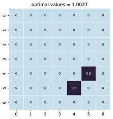
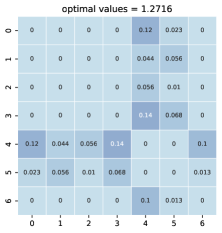
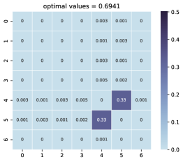
Figure 5: The illustration of how the choice of $s_{u}$ and $s_{v}$ affects the optimal values of $\varphi\circ\pi_{M,\tilde{d}}$. Given fixed $\delta,d,\hat{d}$, we set the optimal values as $\underset{\hat{\mathcal{C}}=[\mathbf{x}_{1},\ldots,\mathbf{x}_{n}]}{\min}\sum_{i<j}\left(\left\|\mathbf{x}_{i}-\mathbf{x}_{j}\right\|-\hat{d}_{ij}\right)^{2}/\delta^{2}$. In each figure, the matrix grids $(i,j)$ denote the entries of $(\operatorname{adj}_{ij}(\mathcal{C})-\hat{d}_{ij})^{2}/\delta^{2}$. We want to minimize the sum of grid values. The left figure denotes the case where we take $\hat{\mathcal{C}}=\tilde{\mathcal{C}}$. In this case, only the entry $(4,5)$ introduces the loss to the optimal value but the value of the entry $(4,5)$ is comparably large. The middle figure denotes the case where we take $s_{u}=s_{v}=\delta/2$. In this case, the value of the entry $(4,5)$ is reduced to zero but other entries become non-zero, and the total loss increases. In the right figure, we take $s_{u}=\delta/(2\operatorname{degree}_{u})$ and $s_{v}=\delta/(2\operatorname{degree}_{v})$. At this time, although the loss introduced by the entry $(u,v)$ is not reduced to $0$, the value of the entry sum is reduced.

When we consider a fully connected graph, $\operatorname{degree}_{u}=\operatorname{degree}_{v}=n-1$ and we have

$$\left\{\begin{aligned} \hat{\mathbf{x}}_{u}&=\tilde{\mathbf{x}}_{u}+\frac{\delta}{2(n-1)}\boldsymbol{\lambda}_{uv},\\ \hat{\mathbf{x}}_{v}&=\tilde{\mathbf{x}}_{v}-\frac{\delta}{2(n-1)}\boldsymbol{\lambda}_{uv},\\ \hat{\mathbf{x}}_{w}&=\tilde{\mathbf{x}}_{w},\quad\quad w\neq u,v,\end{aligned}\right.$$

where $\boldsymbol{\lambda}_{uv}=\frac{\tilde{\mathbf{x}}_{u}-\tilde{\mathbf{x}}_{v}}{\left\|\tilde{\mathbf{x}}_{u}-\tilde{\mathbf{x}}_{v}\right\|}$. We want to write the above equations in a more compact way. Note that

$$(\frac{\partial\tilde{d}_{uv}}{\partial\tilde{\mathcal{C}}})_{u} =(\frac{\partial\|\tilde{\mathbf{x}}_{u}-\tilde{\mathbf{x}}_{v}\|}{\partial\tilde{\mathcal{C}}})_{u}=\frac{\partial\|\tilde{\mathbf{x}}_{u}-\tilde{\mathbf{x}}_{v}\|}{\partial\tilde{\mathbf{x}}_{u}}=\frac{\tilde{\mathbf{x}}_{u}-\tilde{\mathbf{x}}_{v}}{\left\|\tilde{\mathbf{x}}_{u}-\tilde{\mathbf{x}}_{v}\right\|} =\boldsymbol{\lambda}_{uv},$$ (41a)

$$(\frac{\partial\tilde{d}_{uv}}{\partial\tilde{\mathcal{C}}})_{v} =(\frac{\partial\|\tilde{\mathbf{x}}_{u}-\tilde{\mathbf{x}}_{v}\|}{\partial\tilde{\mathcal{C}}})_{v}=\frac{\partial\|\tilde{\mathbf{x}}_{u}-\tilde{\mathbf{x}}_{v}\|}{\partial\tilde{\mathbf{x}}_{v}}=-\frac{\tilde{\mathbf{x}}_{u}-\tilde{\mathbf{x}}_{v}}{\left\|\tilde{\mathbf{x}}_{u}-\tilde{\mathbf{x}}_{v}\right\|} =-\boldsymbol{\lambda}_{uv},$$ (41b)

$$(\frac{\partial\tilde{d}_{uv}}{\partial\tilde{\mathcal{C}}})_{k} =(\frac{\partial\|\tilde{\mathbf{x}}_{u}-\tilde{\mathbf{x}}_{v}\|}{\partial\tilde{\mathcal{C}}})_{k}=\frac{\partial\|\tilde{\mathbf{x}}_{u}-\tilde{\mathbf{x}}_{v}\|}{\partial\tilde{\mathbf{x}}_{k}}=\mathbf{0}, \quad k\neq u,v.$$ (41c)

Hence, we have

$$\hat{\mathcal{C}}=\tilde{\mathcal{C}}+\frac{\delta}{2(n-1)}\frac{\partial\tilde{d}_{uv}}{\partial\tilde{\mathcal{C}}},$$ (42)

where $\hat{\mathcal{C}}=[\hat{\mathbf{x}}_{1},\ldots,\hat{\mathbf{x}}_{n}]^{\top}$. Under such an approximation, the optimal value is bounded by $\frac{2n^{2}-7n+6}{2(n-1)^{2}}\delta^{2}$ and the approximation error does not explode with the increase of node numbers. We refer readers to Appendix D for the proof.

Note that $\hat{\mathcal{C}}$ may not lie in the manifold $N$. We can find an element $\hat{\mathcal{C}_{N}}\in N$ such that $\operatorname{adj}\left(\hat{\mathcal{C}_{N}}\right)=\operatorname{adj}\left(\hat{\mathcal{C}}\right)$ by $\hat{\mathcal{C}_{N}}=\varphi\left(\operatorname{adj}\left(\hat{\mathcal{C}}\right)\right)$. Then, we define $\pi_{N}=\varphi\circ\operatorname{adj}$ and we have

$$\varphi\circ\pi_{M,\tilde{d}}(\tilde{d}+\delta\bar{e}_{uv})\approx\varphi\left(\operatorname{adj}\left(\tilde{\mathcal{C}}+\frac{\delta}{2(n-1)}\frac{\partial\tilde{d}_{uv}}{\partial\tilde{\mathcal{C}}}\right)\right).$$ (43)

By the definition of the differential, $\mathrm{d}\varphi_{\tilde{d}}\left(\gamma^{\prime}(0)\right)=(\varphi\circ\gamma)^{\prime}(0)$, $\mathrm{d}\varphi_{\tilde{d}}$ maps a vector in the tangent space $T_{\tilde{d}}M$ to the tangent space $T_{\tilde{\mathcal{C}}}N$. Again, applying the above approximation for the function $\varphi\circ\pi_{M}$, we have

$$\mathrm{d}\varphi_{\tilde{d}}(\tilde{d}+\delta\bar{e}_{uv})\approx\tilde{\mathcal{C}}+\frac{\delta}{2(n-1)}\frac{\partial\tilde{d}_{uv}}{\partial\tilde{\mathcal{C}}}.$$ (44)

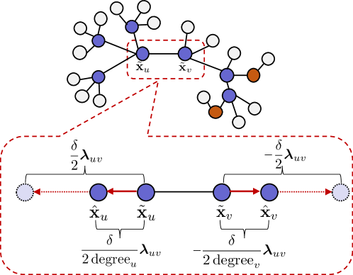
Figure 6: The illustration of approximating the solution of $\varphi\circ\pi_{M}(\tilde{d}+\delta\bar{e}_{uv})$

C.3.3 Generic case of $\varphi\circ\pi_{M}$

In the above section, we approximate the value for $\displaystyle\varphi\circ\pi_{M,\tilde{d}}(\tilde{d}+\delta\bar{e}_{uv})$. In this section, we consider generic cases where $\displaystyle\hat{d}=\tilde{d}+\sum_{i<j}\alpha_{ij}\bar{e}_{ij}\triangleq\tilde{d}+\sum_{i,j}\alpha_{ij}e_{ij}$, where $e_{ij}$ is a zero matrix except for the entry $(i,j)$ and $\alpha_{ij}=\alpha_{ji}$. Consider the mapping $f:T_{\tilde{d}}M\rightarrow N$. There are two ways to transform from $TM$ to $N$. One is by $TM\rightarrow TN\rightarrow N$ and the other one is by $TM\rightarrow M\rightarrow N$. The former transformation is defined by the composition $\pi_{N}\circ\mathrm{d}\varphi$ and the latter by $\varphi\circ\pi_{M}$. Hence, $f=\varphi\circ\pi_{M}=\pi_{N}\circ\mathrm{d}\varphi$. Then, we have

$$\pi_{N}\circ\mathrm{d}\varphi(\tilde{d}+\delta\bar{e}_{uv})=\varphi\circ\pi_{M,\tilde{d}}(\tilde{d}+\delta\bar{e}_{uv})\approx\varphi\circ\operatorname{adj}\left(\tilde{\mathcal{C}}+\frac{\delta}{2(n-1)}\frac{\partial\tilde{d}_{uv}}{\partial\tilde{\mathcal{C}}}\right)$$ (45)

and

$$\varphi\circ\pi_{M,\tilde{d}}(\hat{d}) =\varphi\circ\pi_{M,\tilde{d}}(\tilde{d}+\sum_{i<j}\alpha_{ij}\bar{e}_{ij})$$ (46a)

$$=\pi_{N}\circ\mathrm{d}\varphi_{\tilde{d}}(\tilde{d}+\sum_{i<j}\alpha_{ij}\bar{e}_{ij})\quad\quad (\varphi\circ\pi_{M,\tilde{d}}=\pi_{N}\circ\mathrm{d}\varphi_{\tilde{d}})$$ (46b)

$$=\pi_{N}\left((1-\frac{n^{2}-n}{2})\mathrm{d}\varphi_{\tilde{d}}(\tilde{d})+\sum_{i<j}\mathrm{d}\varphi_{\tilde{d}}(\tilde{d}+\alpha_{ij}\bar{e}_{ij})\right)\quad\quad (\text{differential is linear})$$ (46c)

$$\approx\pi_{N}\left((1-\frac{n^{2}-n}{2})\tilde{\mathcal{C}}+\sum_{i<j}\tilde{\mathcal{C}}+\frac{\alpha_{ij}}{2(n-1)}\frac{\partial\tilde{d}_{ij}}{\partial\tilde{\mathcal{C}}}\right)\quad\quad (\text{induced from Eq.~{}\eqref{eq: differential approximation simple case}})$$ (46d)

$$=\varphi\circ\operatorname{adj}\left(\tilde{\mathcal{C}}+\sum_{i<j}\frac{\alpha_{ij}}{2(n-1)}\frac{\partial\tilde{d}_{ij}}{\partial\tilde{\mathcal{C}}}\right)\quad\quad (\pi_{N}=\varphi\circ\operatorname{adj})$$ (46e)

$$=\varphi\circ\operatorname{adj}\left(\tilde{\mathcal{C}}+\frac{\alpha}{2(n-1)}\circledast\frac{\partial\tilde{d}}{\partial\tilde{\mathcal{C}}}\right)\quad\quad (\text{by Def.~{}\ref{def: matrix2 times matrix4}})$$ (46f)

where $\frac{\partial\tilde{d}}{\partial\tilde{\mathcal{C}}}=\left(\frac{\partial\tilde{d}_{ij}}{\partial\tilde{\mathcal{C}}}\right)_{n\times n}$ and $\alpha=\left(\alpha_{ij}\right)_{n\times n},\alpha_{ij}=\alpha_{ji}$. The formula for $\varphi\circ\pi_{M,\tilde{d}}$ looks complex. In the following, we will show that at the implementation level, we can drop the $\varphi\circ\operatorname{adj}$ term and thus $\displaystyle\varphi\circ\pi_{M,\tilde{d}}(\hat{d})=\tilde{\mathcal{C}}+\frac{\alpha}{2(n-1)}\circledast\frac{\partial\tilde{d}}{\partial\tilde{\mathcal{C}}}$. The function becomes linear.

In the above analysis, we restrict $\hat{\mathcal{C}}$ to be in the manifold of the spectral coordinate manifold $N$. However, in practice, we are not interested in whether $\hat{\mathcal{C}}$ lies in the manifold $N$ or not, as long as the denoising process of the adjacency matrix does not change. Note that the composition function $\varphi\circ\operatorname{adj}$ does not affect the value of the adjacency matrix. Hence, at the implementation level, we can remove this function. Mathematically speaking, given $\tilde{d}^{k}\in M$ and its associated spectral coordinates $\tilde{C}^{k}\in N$, in each update, $\hat{d}^{k-1}=\tilde{d}^{k}-F^{\mathcal{N}}(\tilde{d}^{k},kT/N)$ and we update $\tilde{C}^{k}$ by

$$\tilde{\mathcal{C}}^{k-1}=\varphi\circ\operatorname{adj}\left(\tilde{\mathcal{C}}^{k}-\frac{F^{\mathcal{N}}(\tilde{d}^{k},kT/N)}{2(n-1)}\circledast\frac{\partial\tilde{d}^{k}}{\partial\tilde{\mathcal{C}}^{k}}\right)\simeq\tilde{\mathcal{C}}^{k}-\frac{F^{\mathcal{N}}(\tilde{d}^{k},kT/N)}{2(n-1)}\circledast\frac{\partial\tilde{d}^{k}}{\partial\tilde{\mathcal{C}}^{k}}.$$ (47)

At the implementation level, substituting $F^{\mathcal{N}}$ by Eq. (36), we can update $\gamma_{2}$ or $\mathcal{C}$ by

$$\mathcal{C}^{k-1} =\mathcal{C}^{k}-\frac{F^{\mathcal{N}}(d^{k},kT/N)}{2(n-1)}\circledast\frac{\partial d^{k}}{\partial\mathcal{C}^{k}}$$ (48a)

$$=\mathcal{C}^{k}+\frac{\tau}{2(n-1)}\left(-f(d^{k})+g^{2}(kT/N)\nabla_{d}\log p_{kT/N}(d^{k})\right)\circledast\frac{\partial d^{k}}{\partial\mathcal{C}^{k}}+\frac{\sqrt{\tau}}{2(n-1)}g(kT/N)\mathbf{z}^{k,d^{k}}\circledast\frac{\partial d^{k}}{\partial\mathcal{C}^{k}}.$$ (48b)

C.4 Elimination of functions related to the adjacency matrix

Since we do not know the form of the functions $f$ and $g$, we may consider trying to replace $f$ and $g$ with $\mathbf{f}$ and $\mathbf{G}$, which are the hyperparameters and the noise scheduler on coordinates. Remind that given the forward diffusion process with some specific choice of $\mathbf{f}$ and $\mathbf{G}$ noise scheduler on coordinates by

$$\mathrm{d}\mathcal{C}_{t}=\mathbf{f}(\mathcal{C}_{t},t)\mathrm{d}t+\mathbf{G}(\mathcal{C}_{t},t)\mathrm{d}\mathbf{w},$$ (49)

we denote its associated diffusion of adjacency matrices as

$$\mathrm{d}\gamma_{1}(t)=f(\gamma_{1}(t))\mathrm{d}t+g(t)\mathrm{d}\mathcal{B}_{t}^{M}.$$ (50)

We discretize the above two equations and we have

$$\mathcal{C}^{k+1} =\mathcal{C}^{k}+\tau\mathbf{f}(\mathcal{C}^{k},kT/N)+\sqrt{\tau}\mathbf{G}(\mathcal{C}^{k},kT/N)\mathbf{z}^{k,\mathcal{C}^{k}},$$ (51a)

$$\mathcal{C}^{k+1} =\varphi(d^{k+1})=\varphi\circ\pi_{M,d^{k}}\left(d^{k}+\tau f(d^{k})+\sqrt{\tau}g(kT/N)\mathbf{z}^{k,d^{k}}\right)$$ (51b)

$$=\varphi\circ\operatorname{adj}\left(\mathcal{C}^{k}+\frac{1}{2(n-1)}\left(\tau f(d^{k})+\sqrt{\tau}g(kT/N)\mathbf{z}^{k,d^{k}}\right)\circledast\frac{\partial d_{t}}{\partial\mathcal{C}_{t}}\right)$$ (by Sec. C.3) (51c)

$$=\mathcal{C}^{k}+\frac{1}{2(n-1)}\left(\tau f(d^{k})+\sqrt{\tau}g(kT/N)\mathbf{z}^{k,d^{k}}\right)\circledast\frac{\partial d_{t}}{\partial\mathcal{C}_{t}},$$ (by Def. 7) (51d)

where $\tau=T/N$ and each entry of $\mathbf{z}^{k,\mathcal{C}^{k}}$ and $\mathbf{z}^{k,d^{k}}$ follow the normal distribution. This implies

$$\tau\mathbf{f}(\mathcal{C}^{k},kT/N)+\sqrt{\tau}\mathbf{G}(\mathcal{C}^{k},kT/N)\mathbf{z}^{k,\mathcal{C}^{k}}=\frac{1}{2(n-1)}\left(\tau f(d^{k})+\sqrt{\tau}g(kT/N)\mathbf{z}^{k,d^{k}}\right)\circledast\frac{\partial d_{t}}{\partial\mathcal{C}_{t}}.$$ (52)

Substitute Eq. (48) with the above equation, we have

$$\tilde{\mathcal{C}}^{k-1} =\tilde{\mathcal{C}}^{k}-\left(\tau\mathbf{f}(\mathcal{C}^{k},kT/N)+\sqrt{\tau}\mathbf{G}(\mathcal{C}^{k},kT/N)\mathbf{z}^{k,\mathcal{C}^{k}}\right)+\frac{\tau g^{2}(kT/N)}{2(n-1)}\nabla_{d}\log p_{kT/N}(d^{k})\circledast\frac{\partial d^{k}}{\partial\mathcal{C}^{k}}.$$ (53a)

The above discretization corresponds to the SDE

$$\mathrm{d}\mathcal{C}_{t}=\left(\mathbf{f}(\mathcal{C}_{t},t)-\frac{g^{2}(t)}{2(n-1)}\nabla_{d}\log p_{t}(d_{t})\circledast\frac{\partial d_{t}}{\partial\mathcal{C}_{t}}\right)\mathrm{d}t+\mathbf{G}(\mathcal{C}_{t},t)\mathrm{d}\bar{\mathcal{\mathbf{w}}}.$$ (54)

Hence, in the sampling process, if we can solve Eq. (54), then the obtained $\mathcal{C}_{0}$ has an adjacency matrix $d_{0}=\operatorname{adj}\left(\mathcal{C}_{0}\right)$ follows the distribution of $p_{0}$. However, directly solving Eq. (54) may cost thousands of iterations. In the following, we consider a reverse ODE which has the same marginal distribution as the reverse SDE given by Eq. (54).

C.5 Reverse ODE

C.5.1 Adjacency matrices change along with the perturbation of coordinates

We want to investigate how the adjacency matrices evolve along with the perturbation of coordinates, which will be useful in computing the SDE of the adjacency matrix. We only consider a simple case where the noise is injected on coordinates following the variance exploding noise scheduler. Given a forward diffusion process of the conformation $\tilde{\mathcal{C}}=\mathcal{C}+\mathbf{z}^{\mathcal{C}}\in\mathbb{R}^{n\times 3}$, where $\mathbf{z}_{i}^{\mathcal{C}}\sim\mathcal{N}(\mathbf{0},\sigma^{2}\mathbf{I}_{3\times 3}),i=1,\ldots,n$, we have

$$\tilde{\mathcal{C}}_{u} =\mathcal{C}_{u}+\mathbf{z}_{u}\qquad\tilde{\mathcal{C}}_{v}=\mathcal{C}_{v}+\mathbf{z}_{v}$$ (55a)

$$\tilde{d}_{uv} =\|\tilde{\mathcal{C}}_{u}-\tilde{\mathcal{C}}_{v}\|$$ (55b)

$$=\|\tilde{\mathcal{C}}_{u}-\mathcal{C}_{u}+\mathcal{C}_{u}-\mathcal{C}_{v}+\mathcal{C}_{v}-\tilde{\mathcal{C}}_{v}\|$$ (55c)

$$=\|\mathbf{z}_{u}-\mathbf{z}_{v}+\mathcal{C}_{u}-\mathcal{C}_{v}\|$$ (55d)

$$\simeq\|\mathbf{z}+\mathcal{C}_{u}-\mathcal{C}_{v}\|\quad\quad(\mathbf{z}\sim\mathcal{N}(\mathbf{0},2\sigma^{2}\mathbf{I}_{3\times 3}))$$ (55e)

$$=\|\mathcal{C}_{u}-\mathcal{C}_{v}\|+\|\mathbf{z}+\mathcal{C}_{u}-\mathcal{C}_{v}\|-\|\mathcal{C}_{u}-\mathcal{C}_{v}\|$$ (55f)

$$=\|\mathcal{C}_{u}-\mathcal{C}_{v}\|+(\|\mathbf{z}+\mathcal{C}_{u}-\mathcal{C}_{v}\|-\|\mathcal{C}_{u}-\mathcal{C}_{v}\|)\frac{\|\mathbf{z}+\mathcal{C}_{u}-\mathcal{C}_{v}\|+\|\mathcal{C}_{u}-\mathcal{C}_{v}\|}{\|\mathbf{z}+\mathcal{C}_{u}-\mathcal{C}_{v}\|+\|\mathcal{C}_{u}-\mathcal{C}_{v}\|}$$ (55g)

$$=\|\mathcal{C}_{u}-\mathcal{C}_{v}\|+\frac{\|\mathcal{C}_{u}-\mathcal{C}_{v}\|^{2}+2\mathbf{z}^{\top}(\mathcal{C}_{u}-\mathcal{C}_{v})+\|\mathbf{z}\|^{2}-\|\mathcal{C}_{u}-\mathcal{C}_{v}\|^{2}}{\|\mathbf{z}+\mathcal{C}_{u}-\mathcal{C}_{v}\|+\|\mathcal{C}_{u}-\mathcal{C}_{v}\|}$$ (55h)

$$=\|\mathcal{C}_{u}-\mathcal{C}_{v}\|+\frac{2\mathbf{z}^{\top}(\mathcal{C}_{u}-\mathcal{C}_{v})+\|\mathbf{z}\|^{2}}{\|\mathbf{z}+\mathcal{C}_{u}-\mathcal{C}_{v}\|+\|\mathcal{C}_{u}-\mathcal{C}_{v}\|}$$ (55i)

$$=d_{uv}+\frac{2\mathbf{z}^{\top}(\mathcal{C}_{u}-\mathcal{C}_{v})+\|\mathbf{z}\|^{2}}{\|\mathbf{z}+\mathcal{C}_{u}-\mathcal{C}_{v}\|+\|\mathcal{C}_{u}-\mathcal{C}_{v}\|}$$ (55j)

In terms of the diffusion SDE, given a forward diffusion process on coordinates by

$$\mathrm{d}\mathcal{C}_{t}=\mathbf{G}(t)\mathrm{d}\mathbf{w},$$ (56)

where $\mathbf{G}(t)$ is a scalar function. We discretize the forward diffusion process as

$$\mathcal{C}^{t+\tau}=\mathcal{C}^{t}+\sqrt{\tau}\mathbf{G}(t)\mathbf{z}^{t,\mathcal{C}^{t}},$$ (57)

where $\mathbf{z}^{t,\mathcal{C}^{t}}\in\mathbb{R}^{n\times 3},\mathbf{z}^{t,\mathcal{C}^{t}}_{i}\sim\mathcal{N}(\mathbf{0},\mathbf{I}_{3\times 3})$. Let $\mathbf{m}^{t,\mathcal{C}^{t}}=\sqrt{\tau}\mathbf{G}(t)\mathbf{z}^{t,\mathcal{C}^{t}}$. Consider the associated diffusion of the adjacency matrix $d^{t}=\operatorname{adj}\left(\mathcal{C}^{t}\right)$, we have, for $u\neq v$,

$$\quad d_{uv}^{t}-d_{uv}^{t+\tau}$$ (58a)

$$=d_{uv}^{t}-\operatorname{adj}_{uv}\left(\mathcal{C}^{t}+\mathbf{m}^{t,\mathcal{C}^{t}}\right)$$ (58b)

$$=d_{uv}^{t}-\left[d_{uv}^{t}+\left(2{\mathbf{m}_{uv}^{t}}^{\top}\left(\mathcal{C}_{u}-\mathcal{C}_{v}\right)+\|\mathbf{m}_{uv}^{t}\|^{2}\right)/M_{uv}^{t}\right]$$ (58c)

$$=-\left(2{\mathbf{m}_{uv}^{t}}^{\top}\left(\mathcal{C}_{u}-\mathcal{C}_{v}\right)+\|\mathbf{m}_{uv}^{t}\|^{2}\right)/M_{uv}^{t}$$ (58d)

$$=-2\sqrt{2\tau}\mathbf{G}(t){\mathbf{z}_{uv}^{t}}^{\top}\left(\mathcal{C}_{u}-\mathcal{C}_{v}\right)/M_{uv}^{t}+\left(2\tau\mathbf{G}^{2}(t)\|\mathbf{z}_{uv}^{t}\|^{2}\right)\cdot\left(1/\left(2\|\mathcal{C}_{u}-\mathcal{C}_{v}\|\right)+\lito(\tau^{1/3})\right)$$ (58e)

$$=-2\sqrt{2\tau}\mathbf{G}(t){\mathbf{z}_{uv}^{t}}^{\top}\left(\mathcal{C}_{u}-\mathcal{C}_{v}\right)/M_{uv}^{t}+\tau\mathbf{G}^{2}(t)\|\mathbf{z}_{uv}^{t}\|^{2}/d_{uv}+\lito(\tau)$$ (58f)

where $\mathbf{m}_{uv}^{t}=\sqrt{\tau}\mathbf{G}(t)\left(\mathbf{z}^{t,\mathcal{C}_{u}}-\mathbf{z}^{t,\mathcal{C}_{v}}\right)\triangleq\sqrt{2\tau}\mathbf{G}(t)\mathbf{z}_{uv}^{t},\mathbf{z}_{uv}^{t}\sim\mathcal{N}(\mathbf{0},\mathbf{I}_{3\times 3})$, $M_{uv}^{t}=\|\mathbf{m}_{uv}^{t}+\mathcal{C}_{u}-\mathcal{C}_{v}\|+\|\mathcal{C}_{u}-\mathcal{C}_{v}\|$.

$$\quad\left(d_{uv}^{t}-d_{uv}^{t+\tau}\right)^{2}$$ (59a)

$$=\left(2{\mathbf{m}_{uv}^{t}}^{\top}\left(\mathcal{C}_{u}-\mathcal{C}_{v}\right)+\|\mathbf{m}_{uv}^{t}\|^{2}\right)^{2}/\left(M_{uv}^{t}\right)^{2}$$ (59b)

$$=\left(2{\mathbf{m}_{uv}^{t}}^{\top}\left(\mathcal{C}_{u}-\mathcal{C}_{v}\right)+\|\mathbf{m}_{uv}^{t}\|^{2}\right)^{2}\cdot\left(1/\left(2\|\mathcal{C}_{u}-\mathcal{C}_{v}\|\right)+\lito(\tau^{1/3})\right)^{2}$$ (59c)

$$=4\cdot 2\tau\mathbf{G}^{2}(t)\left({\mathbf{z}_{uv}^{t}}^{\top}\left(\mathcal{C}_{u}-\mathcal{C}_{v}\right)\right)^{2}/\left(4\|\mathcal{C}_{u}-\mathcal{C}_{v}\|^{2}\right)+\lito(\tau)$$ (59d)

$$=2\tau\mathbf{G}^{2}(t)\left({\mathbf{z}_{uv}^{t}}^{\top}\frac{\mathcal{C}_{u}-\mathcal{C}_{v}}{\|\mathcal{C}_{u}-\mathcal{C}_{v}\|}\right)^{2}+\lito(\tau)$$ (59e)

From Eq. (58d) to Eq. (58e) is beacuse if $\mathbf{x}\neq\mathbf{0}$, then

$$\quad\lvert\frac{1}{\|\sqrt{\tau}\mathbf{z}+\mathbf{x}\|+\|\mathbf{x}\|}-\frac{1}{2\|\mathbf{x}\|}\rvert$$ (60a)

$$=\frac{\lvert 2\|\mathbf{x}\|-\|\mathbf{x}\|-\|\sqrt{\tau}\mathbf{z}+\mathbf{x}\|\rvert}{2\|\mathbf{x}\|\left(\|\sqrt{\tau}\mathbf{z}+\mathbf{x}\|+\|\mathbf{x}\|\right)}$$ (60b)

$$\leq\frac{\lvert\|\mathbf{x}\|-\|\sqrt{\tau}\mathbf{z}+\mathbf{x}\|\rvert}{2\|\mathbf{x}\|^{2}}$$ (60c)

$$=\frac{\lvert\|\mathbf{x}\|^{2}-\|\sqrt{\tau}\mathbf{z}+\mathbf{x}\|^{2}\rvert}{2\|\mathbf{x}\|^{2}\left(\|\mathbf{x}\|+\|\sqrt{\tau}\mathbf{z}+\mathbf{x}\|\right)}$$ (60d)

$$\leq\frac{\lvert 2\sqrt{\tau}\mathbf{z}^{\top}\mathbf{x}+\tau\|\mathbf{z}\|^{2}\rvert}{2\|\mathbf{x}\|^{3}}$$ (60e)

$$=\lito(\tau^{1/3})$$ (60f)

We have $\frac{1}{\|\sqrt{\tau}\mathbf{z}+\mathbf{x}\|+\|\mathbf{x}\|}=\frac{1}{2\|\mathbf{x}\|}+\lito(\tau^{1/3})$. Using Eq. (58) and Eq. (59) and approximating $\mathbb{E}[{\mathbf{z}_{uv}^{t}}^{\top}\left(\mathcal{C}_{u}-\mathcal{C}_{v}\right)/M_{uv}^{t}]\approx 0$, directly we have

$$\mathbb{E}_{\mathbf{z}_{uv}^{t}}\left[d_{uv}^{t}-d_{uv}^{t+\tau}\right] \approx-3\tau\mathbf{G}^{2}(t)/d_{uv}^{t}+\lito(\tau),$$ (61a)

$$\mathbb{E}_{\mathbf{z}_{uv}^{t}}\left[\left(d_{uv}^{t}-d_{uv}^{t+\tau}\right)^{2}\right] =2\tau\mathbf{G}^{2}(t)+\lito(\tau).$$ (61b)

Note that there exist an exact solution of $\mathbb{E}_{\mathbf{z}_{uv}^{t}}\left[d_{uv}^{t}-d_{uv}^{t+\tau}\right]$.

$$\quad\mathbb{E}_{\mathbf{z}_{uv}^{t}}\left[d_{uv}^{t}-d_{uv}^{t+\tau}\right]$$ (62a)

$$=\mathbb{E}_{\mathbf{z}_{uv}^{t}}\left[d_{uv}^{t}-\|\mathbf{m}_{uv}^{t}+\mathcal{C}_{u}-\mathcal{C}_{v}\|\right]$$ (62b)

$$=\mathbb{E}_{\mathbf{z}_{uv}^{t}}\left[d_{uv}^{t}-\|\sqrt{2\tau}\mathbf{G}(t)\mathbf{z}_{uv}^{t}+\mathcal{C}_{u}-\mathcal{C}_{v}\|\right]$$ (62c)

$$\triangleq d_{uv}^{t}-\mathbb{E}_{\mathbf{z}_{uv}^{t}}\left[\|X\|\right]$$ (62d)

where $X\triangleq\mathcal{N}(\mathcal{C}_{u}-\mathcal{C}_{v},2\tau\mathbf{G}^{2}(t))$. It is known that if $X\sim\mathcal{N}(\mu,\sigma^{2}\mathbf{I}_{n\times n})$, then $\|X\|/\sigma$ follows a noncentral chi distribution (Park Jr, 1961), which has the mean $\mathbb{E}\|X\|=\sigma\sqrt{\frac{\pi}{2}}L_{1/2}^{(n/2-1)}\left(\frac{-\|\mu\|^{2}}{2\sigma}\right)$, where $L$ is the generalized Laguerre polynomial (Sonine, 1880). Hence, we have

$$\mathbb{E}_{\mathbf{z}_{uv}^{t}}\left[d_{uv}^{t}-d_{uv}^{t+\tau}\right]=\sqrt{\tau\pi}\mathbf{G}(t)L^{1/2}_{1/2}\left(\frac{-\|\mathcal{C}_{u}-\mathcal{C}_{v}\|^{2}}{2\sqrt{2\tau}\mathbf{G}(t)}\right).$$ (63)

C.5.2 Fokker-Planck equation and forward process of the adjacency matrix distribution

To find the reverse ODE which has the same marginal distribution as the forward diffusion, one may consider first deriving the Fokker-Planck equation (Risken & Risken, 1996; Song et al., 2020b). We consider the marginal distribution of the adjacency matrix corresponding to the forward diffusion process of coordinates given by

$$\mathrm{d}\mathcal{C}_{t}=\mathbf{G}(t)\mathrm{d}\mathbf{w},\quad\mathcal{C}^{t+\tau}=\mathcal{C}^{t}+\sqrt{\tau}\mathbf{G}(t)\mathbf{z}^{t,\mathcal{C}^{t}}.$$ (64)

Consider the Dirac delta function

$$\delta\left(d_{uv}-d_{uv}^{t+\tau}\right) =\delta\left(d_{uv}-d_{uv}^{t}+d_{uv}^{t}-d_{uv}^{t+\tau}\right)$$ (65a)

$$=\delta\left(d_{uv}-d_{uv}^{t}\right)+\left(d_{uv}^{t}-d_{uv}^{t+\tau}\right)\nabla_{d_{uv}}\delta\left(d_{uv}-d_{uv}^{t}\right)$$ (65b)

$$\quad+\frac{1}{2}\left(d_{uv}^{t}-d_{uv}^{t+\tau}\right)^{2}\nabla_{d_{uv}}^{2}\delta\left(d_{uv}-d_{uv}^{t}\right)+\lito(\tau)$$

$$p_{t+\tau}\left(d_{uv}\right) =\mathbb{E}_{d_{uv}^{t+\tau}}\left[\delta\left(d_{uv}-d_{uv}^{t+\tau}\right)\right]$$ (66a)

$$=\mathbb{E}_{d_{uv}^{t},\mathbf{m}^{t,\mathcal{C}_{t}}}\left[\delta\left(d_{uv}-d_{uv}^{t}\right)\right]+\mathbb{E}_{d_{uv}^{t},\mathbf{m}^{t,\mathcal{C}_{t}}}\left[\left(d_{uv}^{t}-d_{uv}^{t+\tau}\right)\nabla_{d_{uv}}\delta\left(d_{uv}-d_{uv}^{t}\right)\right]$$ (66b)

$$\quad+\frac{1}{2}\mathbb{E}_{d_{uv}^{t},\mathbf{m}^{t,\mathcal{C}_{t}}}\left[\left(d_{uv}^{t}-d_{uv}^{t+\tau}\right)^{2}\nabla_{d_{uv}}^{2}\delta\left(d_{uv}-d_{uv}^{t}\right)\right]+\lito(\tau)$$

$$=p_{t}(d_{uv})+\mathbb{E}_{d_{uv}^{t}}\left[-3\tau\mathbf{G}^{2}(t)/\|\mathcal{C}_{u}-\mathcal{C}_{v}\|\cdot\nabla_{d_{uv}}\delta\left(d_{uv}-d_{uv}^{t}\right)\right]$$ (66c)

$$\quad+\frac{1}{2}\mathbb{E}_{d_{uv}^{t}}\left[2\tau\mathbf{G}^{2}(t)\cdot\nabla_{d_{uv}}^{2}\delta\left(d_{uv}-d_{uv}^{t}\right)\right]+\lito(\tau)$$

$$=p_{t}(d_{uv})-\nabla_{d_{uv}}\left[3\tau\mathbf{G}^{2}(t)/\|\mathcal{C}_{u}-\mathcal{C}_{v}\|\cdot p_{t}\left(d_{uv}\right)\right]+\tau\mathbf{G}^{2}(t)\cdot\nabla_{d_{uv}}^{2}p_{t}\left(d_{uv}\right)+\lito(\tau)$$ (66d)

Take $\tau\rightarrow 0$, we have

$$\frac{\partial}{\partial t}p_{t}(d_{uv})=-\nabla_{d_{uv}}\left[3\mathbf{G}^{2}(t)/\|\mathcal{C}_{u}-\mathcal{C}_{v}\|\cdot p_{t}\left(d_{uv}\right)\right]+\mathbf{G}^{2}(t)\cdot\nabla_{d_{uv}}^{2}p_{t}\left(d_{uv}\right).$$ (67)

The above Fokker-Planck equation has the solution of the forward diffusion process by (Öttinger, 2012)

$$\mathrm{d}d_{uv}^{t}=3\mathbf{G}^{2}(t)/d_{uv}^{t}\mathrm{d}t+\sqrt{2}\mathbf{G}(t)\mathrm{d}\mathcal{B}_{t}.$$ (68)

C.5.3 Reverse ODE

Note that we can rewrite Eq. (67) as

$$\frac{\partial}{\partial t}p_{t}(d_{uv}) =-\nabla_{d_{uv}}\left[3\mathbf{G}^{2}(t)/\|\mathcal{C}_{u}-\mathcal{C}_{v}\|\cdot p_{t}\left(d_{uv}\right)\right]+\mathbf{G}^{2}(t)\cdot\nabla_{d_{uv}}^{2}p_{t}\left(d_{uv}\right)$$ (69a)

$$=-\nabla_{d_{uv}}\left[3\mathbf{G}^{2}(t)/\|\mathcal{C}_{u}-\mathcal{C}_{v}\|\cdot p_{t}\left(d_{uv}\right)-\left(\mathbf{G}^{2}(t)-\sigma^{2}(t)\right)\nabla_{d_{uv}}p_{t}\left(d_{uv}\right)\right]+\sigma^{2}(t)\cdot\nabla_{d_{uv}}^{2}p_{t}\left(d_{uv}\right)$$ (69b)

$$=-\nabla_{d_{uv}}\left\{\left[3\mathbf{G}^{2}(t)/\|\mathcal{C}_{u}-\mathcal{C}_{v}\|-\left(\mathbf{G}^{2}(t)-\sigma^{2}(t)\right)\nabla_{d_{uv}}\log p_{t}\left(d_{uv}\right)\right]p_{t}\left(d_{uv}\right)\right\}+\sigma^{2}(t)\cdot\nabla_{d_{uv}}^{2}p_{t}\left(d_{uv}\right)$$ (69c)

for any $\sigma(t)\leq\mathbf{G}(t)$. Note that the Eq. (69) has the solution of

$$\mathrm{d}d_{uv}^{t}=\left(3\mathbf{G}^{2}(t)/d_{uv}^{t}-\left(\mathbf{G}^{2}(t)-\sigma^{2}(t)\right)\nabla_{d_{uv}}\log p_{t}\left(d_{uv}^{t}\right)\right)\mathrm{d}t+\sqrt{2}\sigma(t)\mathrm{d}\mathcal{B}_{t}.$$ (70)

The Eq. (68) and Eq. (70) has the same marginal distribution. By setting $\sigma(t)=0$ and ignoring the dependence of entries in the adjacency matrix, the reverse ODE flow is

$$\mathrm{d}\gamma_{1}(t)=\left(3\mathbf{G}^{2}(t)/\gamma_{1}(t)-\mathbf{G}^{2}(t)\nabla_{\gamma_{1}}\log p_{t}\left(\gamma_{1}(t)\right)\right)\mathrm{d}t,$$ (71)

which is the reverse adjacency matrix ODE flow of the Eq. (56). We can write the reverse ODE flow of the coordinates as

$$d^{k-1} =\pi_{M,d^{k}}\left(d^{k}+\tau\left(-3\mathbf{G}^{2}(kT/N)/d^{k}+\mathbf{G}^{2}(kT/N)\nabla_{d}\log p_{kT/N}\left(d^{k}\right)\right)\right)$$ (72a)

$$\mathcal{C}^{k-1} =\varphi\circ\pi_{M,d^{k}}\left(d^{k}+\tau\left(-3\mathbf{G}^{2}(kT/N)/d^{k}+\mathbf{G}^{2}(kT/N)\nabla_{d}\log p_{kT/N}\left(d^{k}\right)\right)\right)$$ (72b)

$$\simeq\mathcal{C}^{k}+\frac{\tau}{2\left(n-1\right)}\left(-3\mathbf{G}^{2}(kT/N)/d^{k}+\mathbf{G}^{2}(kT/N)\nabla_{d}\log p_{kT/N}\left(d^{k}\right)\right)\circledast\frac{\partial d^{k}}{\partial\mathcal{C}^{k}}$$ (72c)

Finally, the above discretization corresponds to the reverse ODE of

$$\frac{\mathrm{d}\mathcal{C}_{t}}{\mathrm{d}t}=\frac{\mathbf{G}^{2}(t)}{2\left(n-1\right)}\left(\frac{3}{d_{t}}-\nabla_{d}\log p_{t}\left(d_{t}\right)\right)\circledast\frac{\partial d_{t}}{\partial\mathcal{C}_{t}}.$$ (73)

Appendix D Error bound analysis

D.1 Error bound computation

We compute the maximum objective function value of $\sum_{i<j}\left(\left\|\hat{\mathbf{x}}_{i}-\hat{\mathbf{x}}_{j}\right\|-\hat{d}_{ij}\right)^{2}$ under our approximation in the case of $\hat{d}=\tilde{d}+\delta e_{uv}$ in Theorem 1. Let $\sim$ denote the adjacent relation and $S_{N}(i)=\{(i,j)\mid\mathbf{x}_{i}\sim\mathbf{x}_{j}\}$ denotes the incident edges of node $i$, $S_{\emptyset}(i,j)=\{(p,q)\mid p\not\in(i,j),q\not\in(i,j)\}$ denote the set of edges that are incident to $i$ and $j$, and $\operatorname{degree}_{i}$ denote the degree of node $i$. We use $\hat{\mathcal{C}}=[\hat{\mathbf{x}}_{1},\ldots,\hat{\mathbf{x}}_{n}]$ to denote our approximated optimal solution, i.e. $\hat{\mathcal{C}}=\tilde{\mathcal{C}}+\frac{\delta}{2(n-1)}\frac{\partial\tilde{d}_{uv}}{\partial\tilde{\mathcal{C}}}$. Formally, we have

$$\quad\quad\quad\quad\quad\quad\min_{\mathbf{x}_{1},\ldots,\mathbf{x}_{n}}\sum_{i<j}\left(\left\|\mathbf{x}_{i}-\mathbf{x}_{j}\right\|-\hat{d}_{ij}\right)^{2}$$ (74a)

$$\leq\left(\left\|\hat{\mathbf{x}}_{u}-\hat{\mathbf{x}}_{v}\right\|-\hat{d}_{uv}\right)^{2}+\sum_{(i,j)\in S_{\emptyset}(u,v)}\left(\left\|\hat{\mathbf{x}}_{i}-\hat{\mathbf{x}}_{j}\right\|-\hat{d}_{ij}\right)^{2}$$ (74b)

$$\quad+\sum_{(i,j)\in S_{N}(u)\setminus\{(u,v)\}}\left(\left\|\hat{\mathbf{x}}_{i}-\hat{\mathbf{x}}_{j}\right\|-\hat{d}_{ij}\right)^{2}+\sum_{(i,j)\in S_{N}(v)\setminus\{(u,v)\}}\left(\left\|\hat{\mathbf{x}}_{i}-\hat{\mathbf{x}}_{j}\right\|-\hat{d}_{ij}\right)^{2}$$

$$=\left(\left\|(\tilde{\mathbf{x}}_{u}+\frac{\delta}{2(n-1)}\boldsymbol{\lambda}_{uv})-(\tilde{\mathbf{x}}_{v}-\frac{\delta}{2(n-1)}\boldsymbol{\lambda}_{uv})\right\|-\tilde{d}_{uv}-\delta\right)^{2}$$ (74c)

$$\quad+\sum_{(i,j)\in S_{\emptyset}(u,v)}\left(\left\|\tilde{\mathbf{x}}_{i}-\tilde{\mathbf{x}}_{j}\right\|-\tilde{d}_{ij}\right)^{2}$$

$$\quad+\sum_{(i,j)\in S_{N}(u)\setminus\{(u,v)\}}\left(\left\|(\tilde{\mathbf{x}}_{u}+\frac{\delta}{2(n-1)}\boldsymbol{\lambda}_{uv})-\tilde{\mathbf{x}}_{j}\right\|-\tilde{d}_{uj}\right)^{2}$$

$$\quad+\sum_{(i,j)\in S_{N}(v)\setminus\{(u,v)\}}\left(\left\|(\tilde{\mathbf{x}}_{v}-\frac{\delta}{2(n-1)}\boldsymbol{\lambda}_{uv})-\tilde{\mathbf{x}}_{j}\right\|-\tilde{d}_{vj}\right)^{2}$$

$$\leq\left(\left\|\boldsymbol{\lambda}_{uv}\left(\left\|\tilde{\mathbf{x}}_{u}-\tilde{\mathbf{x}}_{v}\right\|+\frac{\delta}{n-1}\right)\right\|-\tilde{d}_{uv}-\delta\right)^{2}+0$$ (74d)

$$\quad+\max_{\pm_{(i,j)}}\sum_{(i,j)\in S_{N}(u)\setminus\{(u,v)\}}\left(\left\|\tilde{\mathbf{x}}_{u}-\tilde{\mathbf{x}}_{j}\right\|\pm\left\|\frac{\delta}{2(n-1)}\boldsymbol{\lambda}_{uv}\right\|-\tilde{d}_{uj}\right)^{2}$$

$$\quad+\max_{\pm_{(i,j)}}\sum_{(i,j)\in S_{N}(v)\setminus\{(u,v)\}}\left(\left\|\tilde{\mathbf{x}}_{v}-\tilde{\mathbf{x}}_{j}\right\|\pm\left\|\frac{\delta}{2(n-1)}\boldsymbol{\lambda}_{uv}\right\|-\tilde{d}_{vj}\right)^{2}$$

$$=\left(1-\frac{1}{n-1}\right)^{2}\delta^{2}+\sum_{(i,j)\in S_{N}(u)\setminus\{(u,v)\}}\left(\frac{\delta}{2(n-1)}\right)^{2}+\sum_{(i,j)\in S_{N}(v)\setminus\{(u,v)\}}\left(\frac{\delta}{2(n-1)}\right)^{2}$$ (74e)

$$=\left(\left(\frac{n-2}{n-1}\right)^{2}+\frac{\operatorname{degree}_{u}-1}{4(n-1)^{2}}+\frac{\operatorname{degree}_{v}-1}{4(n-1)^{2}}\right)\delta^{2}$$ (74f)

$$\leq\left(\left(\frac{n-2}{n-1}\right)^{2}+\frac{n-2}{4(n-1)^{2}}+\frac{n-2}{4(n-1)^{2}}\right)\delta^{2}$$ (74g)

$$=\frac{2n^{2}-7n+6}{2(n-1)^{2}}\delta^{2}$$ (74h)

D.2 Experiments of approximated optimal value

Experiment settings.

We randomly generate $\mathcal{C}_{i}\sim\mathcal{N}(\mathbf{0},\boldsymbol{I})$ with $n$ nodes, where $n\sim\operatorname{Uniform}([10,19])$. We compute the adjacency matrix $d$ of the obtained coordinates and randomly perturb the adjacency matrix to obtain $\hat{d}=d+\delta\bar{e}_{uv}$. We aim to compare the magnitude of the optimal values computed under different algorithms or approximations. The optimal value is defined as the solution of the optimization problem $f(\hat{d})=\underset{\hat{\mathbf{x}}_{1},\ldots,\hat{\mathbf{x}}_{n}}{\min}\sum_{i<j}\left(\left\|\hat{\mathbf{x}}_{i}-\hat{\mathbf{x}}_{j}\right\|-\hat{d}_{ij}\right)^{2}$.

Algorithms.

To our best knowledge, there is no simple algorithm for solving the metric MDS problem $\hat{\mathbf{x}}_{1},\ldots,\hat{\mathbf{x}}_{n}=\underset{\hat{\mathbf{x}}_{1},\ldots,\hat{\mathbf{x}}_{n}}{\operatorname{argmin}}\sum_{i<j}\left(\left\|\hat{\mathbf{x}}_{i}-\hat{\mathbf{x}}_{j}\right\|-\hat{d}_{ij}\right)^{2}$. The usual gradient descent algorithm is inapplicable in such case since $\|\mathbf{x}\|$ is not differentiable at $\mathbf{x}=\mathbf{0}$. Usual convergence theorems for gradient methods are invalid under such cases and local minimum points do not need to satisfy the stationary equations (De Leeuw, 2005). Hence, we slightly modify the gradient descent process to

$$\hat{C}^{(t+1)}=\hat{C}^{(t)}+\nabla_{\hat{C}^{(t)}}\sum_{i<j}\left(\left(\left\|\hat{\mathbf{x}}_{i}^{(t)}-\hat{\mathbf{x}}_{j}^{(t)}\right\|^{2}+\epsilon\right)^{1/2}-\hat{d}_{ij}\right)^{2},$$ (75)

for some sufficiently small $\epsilon>0$. From experimental results, the above methods can monotonically decrease the loss when the step size is chosen properly and when $\hat{x}$ is not very close to the local minimum. We set $\hat{C}^{(0)}=\tilde{C}=[\tilde{\mathbf{x}}_{1},\ldots,\tilde{\mathbf{x}}_{n}]$ as the initialized value and apply the gradient descent algorithm. We visualize the magnitude of the MDS objective function obtained at $\hat{\mathcal{C}}_{\textsubscript{approx}},\hat{\mathcal{C}}_{\textsubscript{G}},\hat{\mathcal{C}}_{\textsubscript{c-MDS}}$, computed from the proposed approximation (Eq. (42)), gradient descent (Eq. (75)) and the algorithm for the classic MDS problem, respectively. We also visualize the error bound proved in Theorem 1. The results can be seen in Fig. 7. The algorithm for the classic MDS problem (c-MDS) is stated below (Wickelmaier, 2003):

• Set up the squared proximity matrix $D=\left(d_{ij}^{2}\right)_{n\times n}$.

• Apply double centering: $B=-\frac{1}{2}PDP$ using the centering matrix $P=I-\frac{1}{n}J_{n}$, where $n$ is the number of objects, $I$ is the $n\times n$ identity matrix, and $J_{n}$ is an $n\times n$ matrix of all ones.

• Determine the 3 largest eigenvalues $\lambda_{1},\lambda_{2},\lambda_{3}$ and corresponding eigenvectors $e_{1},e_{2},e_{3}$ of $B$.

• Now, $\mathcal{C}=E_{3}\Lambda_{3}^{1/2}$, where $E_{3}$ is the matrix of $3$ eigenvectors and $\Lambda_{3}$ is the diagonal matrix of $3$ eigenvalues of $B$.

Metric MDS and c-MDS seek to find $\mathcal{C}=[\mathbf{x}_{1},\ldots,\mathbf{x}_{n}]$ such that $\|\mathbf{x}_{i}-\mathbf{x}_{j}\|\approx d_{ij}$ but the optimal solution of c-MDS generally differs from the metric MDS.

Experimental results.

We see that our approximation leads to a much smaller loss than the c-MDS’s, and compared with the optimal value, the gap is acceptable. As there is still improvement for optimal values, this further suggests that applying a more refined projection operator can yield additional improvements in the model’s performance (Zhou & Yu, 2023).

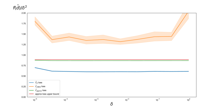
Figure 7: Optimization loss of MDS w.r.t. different optimization algorithm. $f(\hat{d})$ is the objective function of the optimization problem.

Appendix E Corrector analysis

E.1 Reasons for introduction of the corrector

For simplicity, we consider the revised version of the reverse ODE given by Eq. (23). Suppose that we have a model $\mathbf{s}_{\boldsymbol{\theta}}(d_{t},t)=\frac{1}{2(n-1)}\nabla_{d}\log p_{t}\left(d_{t}\right)\circledast\frac{\partial d_{t}}{\partial\mathcal{C}_{t}}+\boldsymbol{\epsilon}(d_{t},t)$, where $\boldsymbol{\epsilon}(d_{t},t)$ is the prediction error from the approximation of 1) the mappings between the adjacency matrix, coordinates, 2) distance distribution, and 3) ignoration of dependence of distance entries. We assume $\boldsymbol{\epsilon}(d_{t},t)$ follows a Gaussian distribution. Consider the discretization of reverse ODE between the timestamp from $s$ to $t$ (note that in variance exploding SDEs, $\mathbf{G}^{2}(t)=\frac{\mathrm{d}\sigma^{2}(t)}{\mathrm{d}t}$):

$$\mathcal{C}_{t} =\mathcal{C}_{s}-\int_{s}^{t}\frac{\mathbf{G}^{2}(u)}{2(n-1)}\nabla_{d}\log p_{u}\left(d_{u}\right)\circledast\frac{\partial d_{u}}{\partial\mathcal{C}_{u}}\mathrm{d}u$$ (76a)

$$\approx\mathcal{C}_{s}+\left(\sigma^{2}(s)-\sigma^{2}(t)\right)\mathbf{s}_{\boldsymbol{\theta}}(d_{s},s)+\left(\sigma^{2}(t)-\sigma^{2}(s)\right)\boldsymbol{\epsilon}(d_{s},s)$$ (76b)

The term $\left(\sigma^{2}(t)-\sigma^{2}(s)\right)\boldsymbol{\epsilon}(d_{s},s)$ can be seen as an addtional noise injected to $\mathcal{C}_{s}$. Hence, after one iteration of the denoising process, the obtained $\tilde{C}_{t}$ does not exactly follow the distribution $q_{t}$ but follows $q_{t+\lambda(s-t)}$ for some $\lambda\in(0,1)$. As the magnitude of the prediction error increases, the corresponding value of the parameter $\lambda$ exhibits a proportional augmentation. This motivates us to choose a larger drift. Hence, we introduce a multiplier “corrector” $k_{\mathbf{s}_{\boldsymbol{\theta}}}(d_{s},s,t)>1$ as an addition term to remedy the model’s prediction errors, and the iteration rule becomes

$$\mathcal{C}_{t} \approx\mathcal{C}_{s}+k_{\mathbf{s}_{\boldsymbol{\theta}}}(d_{s},s,t)\left(\sigma^{2}(s)-\sigma^{2}(t)\right)\mathbf{s}_{\boldsymbol{\theta}}(d_{t},t).$$ (77)

E.2 Experiments

To find the corrector $k_{\mathbf{s}_{\boldsymbol{\theta}}}$, we further assume $k_{\mathbf{s}_{\boldsymbol{\theta}}}(d_{s},s,t)\approx k_{\mathbf{s}_{\boldsymbol{\theta}}}(p_{\textsuperscript{data}})$, i.e., for each dataset, we can find a hyper-parameter to approximate $k_{\mathbf{s}_{\boldsymbol{\theta}}}(d_{s},s,t)$ for all $d_{t}\sim p_{t}(d_{t})$. From the experimental results, we find that the magnitude of $k_{\mathbf{s}_{\boldsymbol{\theta}}}$ increases along with the increase of the model’s prediction error, while other factors such as node number and node degree do not have a significant influence on the choice of $k_{\mathbf{s}_{\boldsymbol{\theta}}}$.

E.2.1 Experiments for positive correlation between prediction error and corrector $k_{\mathbf{s}_{\theta}}$

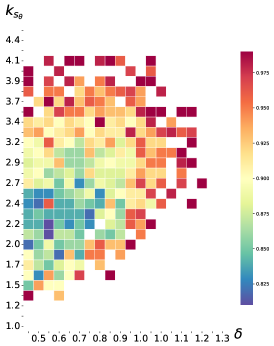
Figure 8: Relations between the prediction error $\delta$ and corrector $k_{\mathbf{s}_{\theta}}$. Grid color indicates the convergent time.

Dataset settings.

We develop datasets $Q_{i}=\{\mathcal{C}_{0}^{(i)}\}$ that only contain one set of coordinates of 20 nodes. Each conformation is a 4-regular graph (so that SE(3)-invariant conformation and pairwise distance manifolds are bijective) and $\mathcal{C}_{0}^{(i)}\sim\mathcal{N}(\mathbf{0},\mathbf{I}),\forall i=1,\ldots,n$. Thus, the ground truth of the denoising process is fixed. We try to sample 3D coordinates in 100 steps.

Model settings.

During the denoising process, our model has access to the ground truth $d_{0}$ and following the Gaussian assumption of the distance distribution, we want to develop a model $\mathbf{s}_{\boldsymbol{\theta}}(d_{t},t)=\frac{1}{2\cdot\operatorname{degree}}\nabla_{d}\log p_{t}\left(d_{t}\right)\circledast\frac{\partial d_{t}}{\partial\mathcal{C}_{t}}$. As discussed in Eq. (76), we cannot access the accurate information about the denoising timestamp during the denoising process, hence, we assume that $\mathbf{s}_{\boldsymbol{\theta}}(d_{t},t)$ has the standard deviation (std) to be 1. Such assumption comes from the fact that the standard deviation of the score matching ground truth $\frac{1}{2\cdot\operatorname{degree}}\nabla_{d}\log p_{t}\left(d_{t}\mid d_{0}\right)\circledast\frac{\partial d_{t}}{\partial\mathcal{C}_{t}}$ approximately equals 1. Thus, the obtained model trends to output a score whose std equals 1. So, we force the output std of our model to be 1. Also, we use a hyperparameter $\delta$ to add prediction errors by letting $\mathbf{s}_{\boldsymbol{\theta}}(d_{t},t,\delta)=\operatorname{Norm}_{\textsubscript{std}}\left(\frac{1}{2\cdot\operatorname{degree}}\nabla_{d}\log p_{t}\left(d_{t}\right)\circledast\frac{\partial d_{t}}{\partial\mathcal{C}_{t}}+\boldsymbol{\epsilon}^{d}(\delta,t)\right)$. But note that when $\delta=0$, there are still prediction errors due to the approximated transformation between distances and coordinates and the inaccurate distance distribution hypothesis. Finally, we define $\boldsymbol{\epsilon}^{d}(\delta,t)=2(\operatorname{sigmoid(\sigma_{t}\cdot\delta)-0.5})\delta\mathbf{z}$, where $\mathbf{z}\sim\mathcal{N}(\mathbf{0},\mathbf{I})$.

Detailed settings of convergence.

We find that even with access to the ground truth of $d_{0}$, our model cannot always converge to the ground truth at the end of the reverse process. Hence, we only consider the convergence for most samples (90% samples). Given a noise level $\delta$ and $k_{\mathbf{s}_{\theta}}$, we repeatedly apply the denoising process. If at time $t_{0}$, at least 90% samples have converged, then we say that under $\delta,k_{\mathbf{s}_{\theta}}$, the model converges at time $t_{0}$.

If $\|d_{t}-d_{0}\|_{\infty}<h$ for some predefined threshold $h>0$, we say that the reverse process converges at $t$ and define the minimal $1-t/T$ to be the convergent time. We aim to find the convergent time under different noise levels $\delta$ and corrector $k_{\mathbf{s}_{\theta}}$. We grid-search the above two parameters and visualize the convergence of the model. The results can be seen in Fig. 8 and the color of each grid represents the convergent time. Grids with no color imply that under such noise level $\delta$ and model error $k_{\mathbf{s}_{\theta}}$, the model diverges. We can see a positive correlation between the model’s error and the corrector, which matches the hypothesis in Eq. (76).

E.2.2 Ablation study on factors influencing the value of the corrector

In the context of our investigation, we employ $\|d_{t}-d_{0}\|_{\infty}$ as a reduced-dimensional representation of the reverse flow phenomenon, where $d_{t}$ denotes the edge lengths of the graph at time $t$, $d_{0}$ denotes the ground truth edge lengths and $\|\cdot\|_{\infty}$ denotes the maximum difference. It is well-established that the selection of the corrector $k_{\mathbf{s}_{\theta}}$ exerts a notable influence on the characteristics of the flow. Our primary objective is to systematically investigate whether while maintaining a constant corrector parameter $k_{\mathbf{s}_{\theta}}$, other variables such as the number of nodes and node degrees exhibit substantial alterations in the reverse flow patterns. Should our findings indicate minimal variation in the reverse flow with respect to these aforementioned factors, it would enable us to posit that the choice of corrector $k_{\mathbf{s}_{\theta}}$ is relatively independent of their influence. We use the same settings of the sigma scheduler and the model, as discussed in the Appendix E.2.1 but develop different toy datasets that contain graphs of distinct node numbers and distinct node degrees.

Dataset settings.

We develop two datasets with one containing a fixed node number of [10, 20, 50, 100], and each graph is a 4-regular graph and the other contains conformations of 20 nodes, and each graph is a $k$-regular graph, where $k=4,5,6$.

Experimental results.

We visualize the flow (represented by $\|d_{t}-d_{0}\|_{\infty}$) under different node numbers and node degrees and find that these two factors have a limited effect on the flow when the corrector $k_{\mathbf{s}_{\theta}}$ is fixed. Results can be seen in Fig. LABEL:fig:_ablation-atom and Fig. LABEL:fig:_ablation-k. We also visualize the reverse flow of 4-regular graphs with 20 nodes under different prediction errors. Results are shown in Fig. LABEL:fig:_ablation-noise. Compared with Fig. LABEL:fig:_ablation-atom and Fig. LABEL:fig:_ablation-k, we can see that the flow under different settings of the model’s error shows great difference and we conclude that prediction error is the main factor that affects the choice of corrector $k_{\mathbf{s}_{\theta}}$.

Appendix F Experiment extension

In this section, we introduce training details first, and then provide more analysis and results for molecular conformation generation task and human pose generation task, respectively.

F.1 Training details

Backbone.

Our two tasks can both be viewed as generating 3D coordinates based on a given graph. A molecule is natural to be represented as a graph. Notably, we add “virtual edges” between nodes that are not originally bonded. Note that we find that embedding time causes a decrease in performance. Hence, we do not embed the diffusion time stamp in the model.

For the molecular generation task, the molecules can be viewed as both local and global components. Same as Xu et al. (2022), we utilize GIN (Xu et al., 2018) to process the local part of the graph and SchNet (Schütt et al., 2017) for the global part. These two models can ensure Permutation Invariance and Graph Isomorphism, which can be beneficial to capturing intricate dependencies within complex graph data.

For the human pose generation task, we conceptualize human pose as a graph where nodes represent key points, and edges signify human limbs. Each node contains 3D coordinates. We perform a normalization of 3D coordinates and then introduce “virtual edges” to guarantee full connectivity within the graph. The graph This adjustment is essential since we consider that each particle requires at least four connections to determine its position, as illustrated in Fig. 11.

Since the backbone we use is a graph neural network, we believe that it is beneficial to add additional edges to the original graph, which not only provides more global information for local nodes but also can better generate high-quality samples with more stability due to the strong connectivity between nodes.

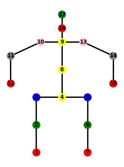
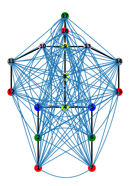
Figure 11: We conceptualize human pose as a graph where nodes represent key points, and edges represent human limbs shown as the left figure; we add “virtual edges” to guarantee full connectivity within the graph shown as the right figure where the blue edges are new-added “virtual edges”.

Configuration.

We trained the model on a single NVIDIA GeForce RTX 3090 GPU and Intel(R) Xeon(R) Silver 4210R CPU @ 2.40GHz CPU. We use the Adam optimizer for training, with a maximum of 1000 epochs. We set the learning rate to 0.001, and it decreases by a factor of 0.6 every 2 epochs. The batch size is 64. As for diffusion configuration, we set the steps of the forward diffusion process to 5000, the noise scheduler to $\sigma_{t}=\sqrt{\frac{\bar{\alpha}_{t}}{1-\bar{\alpha}_{t}}}$ where $\bar{\alpha}_{t}=\prod_{i}^{t}(1-\beta_{i})$ and $\beta_{t}=\operatorname{sigmoid}(t)$. $t$ is uniformly selected in [1e-7, 2e-3], and the magnitude of $\sigma_{t}$ is in the range of 0 to around 12.

F.2 Molecular conformation generation

F.2.1 Evaluation

We use the COV and MAT metrics for Recall (R) and Precision (P) to evaluate the diversity and quality of generated conformers. These metrics are built on the root-mean-square-deviation (RMSD) of heavy atoms. COV can reflect the converge status of ground truth conformers, and MAT denotes the average minimum RMSD. The calculation for COV-R and MAT-R is:

$$\operatorname{COV-R}=\frac{1}{|S_{r}|}\{\mathcal{C}\in S_{r}|\operatorname{RMSD}(\mathcal{C},\mathcal{C}^{\prime})<\tau,\exists\mathcal{C}^{\prime}\in S_{g}\},\quad\operatorname{MAT-R}=\frac{1}{|S_{r}|}\sum_{\mathcal{C}\in S_{r}}\min_{\mathcal{C}^{\prime}\in S_{g}}\operatorname{RMSD}(\mathcal{C},\mathcal{C}^{\prime})$$

where $S_{g}$ and $S_{r}$ denote generated and ground truth conformations. Sweeping $S_{g}$ and $S_{r}$, we obtain the COV-P and MAT-P. The MAT is calculated under RMSD threshold $\tau$. Following previous work (Xu et al., 2020, 2022), we set $\tau=0.5$\text{\,}\mathrm{\SIUnitSymbolAngstrom}$$ for GEOM-QM9 and $\tau=1.25$\text{\,}\mathrm{\SIUnitSymbolAngstrom}$$ for GEOM-Drugs. Different from the previous work, when iterations for sampling are reduced, there may be nan in the generated samples, resulting in MAT metric exploding. Hence, when a sample contains nans, we use another sample from the same conditional generation process to replace it.

F.2.2 Hyper-parameter analysis

In Section E, a hyper-parameter known as the “corrector”, denoted as $k_{\mathbf{s}_{\theta}}$, is introduced. In this section, we report the performance implications associated with varying $k_{\mathbf{s}_{\theta}}$ values. The results for different $k_{\mathbf{s}_{\theta}}$ values are displayed in Table F.2.2. Analysis of these results indicates satisfactory performance for $k_{\mathbf{s}_{\theta}}$ values ranging approximately from 8 to 16, for both the QM9 and Drugs datasets, suggesting a relative insensitivity of our proposed SDE and ODE to variations in the corrector values.

Table 3: Influence of corrector values on our proposed SDE and ODE in Drugs and QM9 dataset. Higher values for COV indicate that the model can generate samples with higher diversity. Lower values for MAT imply the model can generate high-quality samples with lower differences compared with the ground truth samples.

To facilitate a fair comparison with our approach and ensure robust validation, we have conducted a thorough examination of the optimal step size $\alpha_{t}$, as delineated in Eq. 24, for the baseline method, LD. Detailed results of the LD sampling over 100 steps on the QM9 dataset are presented in Table 4. Additionally, the results for LD sampling over 5000 and 1000 steps, as reported in the GeoDiff study, are included for reference in Table 1.

Table 4: Influence of step size variation on sampling via LD over 100 steps in QM9 dataset.

Step size	COV-R(%) $\uparrow$		MAT-R($\text{\,}\mathrm{\SIUnitSymbolAngstrom}$) $\downarrow$		COV-P(%) $\uparrow$		MAT-P($\text{\,}\mathrm{\SIUnitSymbolAngstrom}$) $\downarrow$
	Mean	Median	Mean	Median	Mean	Median	Mean	Median
3e-7	16.57	09.34	0.6573	0.6318	03.19	01.75	1.6711	1.5551
4e-7	76.70	81.61	0.3998	0.3947	31.52	27.16	0.6954	0.6308
5e-7	88.40	91.70	0.3135	0.3120	48.84	47.00	0.5411	0.5024
6e-7	88.88	91.83	0.2898	0.2962	53.48	51.64	0.5051	0.4663
7e-7	88.24	91.08	0.2787	0.2898	54.61	52.00	0.4932	0.4581
8e-7	88.07	90.20	0.2711	0.2808	54.80	52.42	0.5090	0.4552
9e-7	87.22	89.42	0.2695	0.2763	54.87	51.73	0.5364	0.4600
1e-6	87.10	90.73	0.2663	0.2759	54.75	53.01	0.5576	0.4667
2e-6	83.00	87.88	0.2849	0.2858	49.91	45.83	1.5991	0.6705
3e-6	75.22	79.81	0.3460	0.3323	37.64	33.92	-	-
4e-6	65.99	73.94	-	0.3647	31.54	26.74	-	-

F.2.3 Visualization

For qualitative analysis, we visualized conformers generated using our methods over 100 and 1000 steps, as depicted in Fig. LABEL:fig:_vis-mol. These visualizations demonstrate that most molecular structures sampled through our approach are both meaningful and stable, even with a limited step count of only 100.

In Fig. LABEL:fig:_mol-traj, we depict the sampling trajectories of conformers using our proposed SDE and ODE over 100 and 1000 steps. Analysis reveals that conformers’ basic structures are established in the initial half of the process, with only minor adjustments occurring in later steps. This pattern suggests the potential for developing a more expedited sampling method.

F.3 Human pose generation

F.3.1 Hyper-parameter analysis for human pose

For the human pose generation task, we conduct a hyperparameter analysis akin to that in Sec. F.2.2, assessing both our SDE/ODE methods and LD. The AD scores are depicted in Fig. 13. We observe that for our SDE/ODE sampling method, too large a corrector size fails to generate in small steps and also makes the generated results quite unsatisfactory when the number of steps is large. We choose 8-24 as the search range and find that the corrector size from an appropriate range does not have a large impact on the generated results. For LD, a grid search determines that the step size $\alpha_{t}$ has a minimal impact on the performance of LD in this context. Excessively large values for step size also lead to failure in generation.

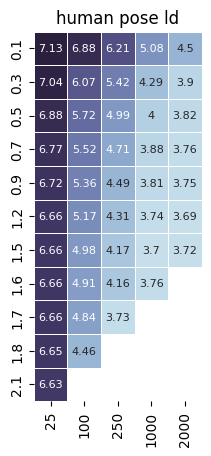
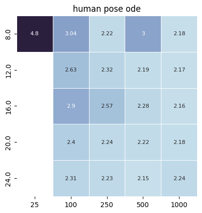
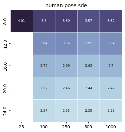
Figure 13: Hyperparameter analysis for human pose task. We investigate the influence of step size variation on sampling via LD and the influence of corrector on proposed SDE and ODE. The horizontal axis represents the number of steps, and the vertical axis represents the value of step size (for LD) or the corrector (for SDE/ODE). Under large values of step size and corrector, the generated human pose can be Nan, resulting unavailable AD score which is shown by the blank cells in the figure.

F.3.2 Visualization of more samples

In this section, we visualize more samples. All the poses are generated from the “eating” action, and we show 36 sampling results of each sampling method in various steps. It is observed that LD fails to yield meaningful structures with a small number of steps. However, when the step count exceeds 2000, LD consistently produces reasonable human structures. In contrast, our proposed SDE and ODE can generate meaningful structures in a small number of steps, as few as 50 or 25 steps.

References

- Anand & Achim (2022) Anand, N. and Achim, T. Protein structure and sequence generation with equivariant denoising diffusion probabilistic models. arXiv preprint arXiv:2205.15019, 2022.
- Axelrod & Gomez-Bombarelli (2022) Axelrod, S. and Gomez-Bombarelli, R. Geom, energy-annotated molecular conformations for property prediction and molecular generation. Scientific Data, 9(1):185, 2022.
- Chambolle & Pock (2019) Chambolle, A. and Pock, T. Total roto-translational variation. Numerische Mathematik, 142:611–666, 2019.
- De Bortoli et al. (2022) De Bortoli, V., Mathieu, E., Hutchinson, M., Thornton, J., Teh, Y. W., and Doucet, A. Riemannian score-based generative modelling. Advances in Neural Information Processing Systems, 35:2406–2422, 2022.
- De Leeuw (2005) De Leeuw, J. Applications of convex analysis to multidimensional scaling. 2005.
- Dormand & Prince (1980) Dormand, J. R. and Prince, P. J. A family of embedded runge-kutta formulae. Journal of computational and applied mathematics, 6(1):19–26, 1980.
- Fan et al. (2023a) Fan, W., Liu, C., Liu, Y., Li, J., Li, H., Liu, H., Tang, J., and Li, Q. Generative diffusion models on graphs: Methods and applications. arXiv preprint arXiv:2302.02591, 2023a.
- Fan et al. (2023b) Fan, Z., Yang, Y., Xu, M., and Chen, H. Ec-conf: A ultra-fast diffusion model for molecular conformation generation with equivariant consistency. arXiv preprint arXiv:2308.00237, 2023b.
- Ganea et al. (2021) Ganea, O., Pattanaik, L., Coley, C., Barzilay, R., Jensen, K., Green, W., and Jaakkola, T. Geomol: Torsional geometric generation of molecular 3d conformer ensembles. Advances in Neural Information Processing Systems, 2021.
- Gasteiger et al. (2020) Gasteiger, J., Groß, J., and Günnemann, S. Directional message passing for molecular graphs. arXiv preprint arXiv:2003.03123, 2020.
- Gilmer et al. (2017) Gilmer, J., Schoenholz, S. S., Riley, P. F., Vinyals, O., and Dahl, G. E. Neural message passing for quantum chemistry. In International conference on machine learning, pp. 1263–1272. PMLR, 2017.
- Gower (1982) Gower, J. C. Euclidean distance geometry. Math. Sci, 7(1):1–14, 1982.
- Ho et al. (2020) Ho, J., Jain, A., and Abbeel, P. Denoising diffusion probabilistic models. Advances in neural information processing systems, 2020.
- Hoffmann & Noé (2019) Hoffmann, M. and Noé, F. Generating valid euclidean distance matrices. arXiv preprint arXiv:1910.03131, 2019.
- Ionescu et al. (2013) Ionescu, C., Papava, D., Olaru, V., and Sminchisescu, C. Human3. 6m: Large scale datasets and predictive methods for 3d human sensing in natural environments. IEEE transactions on pattern analysis and machine intelligence, 36(7):1325–1339, 2013.
- Iskakov et al. (2019) Iskakov, K., Burkov, E., Lempitsky, V., and Malkov, Y. Learnable triangulation of human pose. In Proceedings of the IEEE/CVF international conference on computer vision, pp. 7718–7727, 2019.
- Jing et al. (2022) Jing, B., Corso, G., Chang, J., Barzilay, R., and Jaakkola, T. Torsional diffusion for molecular conformer generation. In Advances in Neural Information Processing Systems, 2022.
- Kocabas et al. (2019) Kocabas, M., Karagoz, S., and Akbas, E. Self-supervised learning of 3d human pose using multi-view geometry. In Proceedings of the IEEE/CVF conference on computer vision and pattern recognition, pp. 1077–1086, 2019.
- Lu et al. (2022a) Lu, C., Zhou, Y., Bao, F., Chen, J., Li, C., and Zhu, J. Dpm-solver: A fast ode solver for diffusion probabilistic model sampling in around 10 steps. In Advances in Neural Information Processing Systems, 2022a.
- Lu et al. (2022b) Lu, C., Zhou, Y., Bao, F., Chen, J., Li, C., and Zhu, J. Dpm-solver++: Fast solver for guided sampling of diffusion probabilistic models. arXiv preprint arXiv:2211.01095, 2022b.
- Luo & Hu (2021) Luo, S. and Hu, W. Diffusion probabilistic models for 3d point cloud generation. In Proceedings of the IEEE/CVF Conference on Computer Vision and Pattern Recognition, pp. 2837–2845, 2021.
- Luo et al. (2021) Luo, S., Shi, C., Xu, M., and Tang, J. Predicting molecular conformation via dynamic graph score matching. In Advances in Neural Information Processing Systems, 2021.
- Mo et al. (2023) Mo, S., Xie, E., Chu, R., Yao, L., Hong, L., Nießner, M., and Li, Z. Dit-3d: Exploring plain diffusion transformers for 3d shape generation. arXiv preprint arXiv:2307.01831, 2023.
- Moré & Wu (1999) Moré, J. J. and Wu, Z. Distance geometry optimization for protein structures. Journal of Global Optimization, 15:219–234, 1999.
- Öttinger (2012) Öttinger, H. C. Stochastic processes in polymeric fluids: tools and examples for developing simulation algorithms. Springer Science & Business Media, 2012.
- Park Jr (1961) Park Jr, J. Moments of the generalized rayleigh distribution. Quarterly of Applied Mathematics, 19(1):45–49, 1961.
- Risken & Risken (1996) Risken, H. and Risken, H. Fokker-planck equation. Springer, 1996.
- Schoenberg (1935) Schoenberg, I. J. Remarks to maurice frechet’s article“sur la definition axiomatique d’une classe d’espace distances vectoriellement applicable sur l’espace de hilbert. Annals of Mathematics, pp. 724–732, 1935.
- Schütt et al. (2017) Schütt, K., Kindermans, P.-J., Sauceda Felix, H. E., Chmiela, S., Tkatchenko, A., and Müller, K.-R. Schnet: A continuous-filter convolutional neural network for modeling quantum interactions. In Advances in neural information processing systems, 2017.
- Shi et al. (2021) Shi, C., Luo, S., Xu, M., and Tang, J. Learning gradient fields for molecular conformation generation. In International Conference on Machine Learning, 2021.
- Song et al. (2020a) Song, J., Meng, C., and Ermon, S. Denoising diffusion implicit models. arXiv preprint arXiv:2010.02502, 2020a.
- Song & Ermon (2019) Song, Y. and Ermon, S. Generative modeling by estimating gradients of the data distribution. In Advances in neural information processing systems, 2019.
- Song et al. (2020b) Song, Y., Sohl-Dickstein, J., Kingma, D. P., Kumar, A., Ermon, S., and Poole, B. Score-based generative modeling through stochastic differential equations. arXiv preprint arXiv:2011.13456, 2020b.
- Song et al. (2023) Song, Y., Dhariwal, P., Chen, M., and Sutskever, I. Consistency models. arXiv preprint arXiv:2303.01469, 2023.
- Sonine (1880) Sonine, N. Recherches sur les fonctions cylindriques et le développement des fonctions continues en séries. Mathematische Annalen, 16(1):1–80, 1880.
- Wen et al. (2021) Wen, C., Yu, B., and Tao, D. Learning progressive point embeddings for 3d point cloud generation. In Proceedings of the IEEE/CVF Conference on Computer Vision and Pattern Recognition, pp. 10266–10275, 2021.
- Wickelmaier (2003) Wickelmaier, F. An introduction to mds. Sound Quality Research Unit, Aalborg University, Denmark, 46(5):1–26, 2003.
- Wu et al. (2016) Wu, J., Zhang, C., Xue, T., Freeman, B., and Tenenbaum, J. Learning a probabilistic latent space of object shapes via 3d generative-adversarial modeling. In Advances in neural information processing systems, volume 29, 2016.
- Xu et al. (2018) Xu, K., Hu, W., Leskovec, J., and Jegelka, S. How powerful are graph neural networks? In International Conference on Learning Representations, 2018.
- Xu et al. (2020) Xu, M., Luo, S., Bengio, Y., Peng, J., and Tang, J. Learning neural generative dynamics for molecular conformation generation. In International Conference on Learning Representations, 2020.
- Xu et al. (2022) Xu, M., Yu, L., Song, Y., Shi, C., Ermon, S., and Tang, J. Geodiff: A geometric diffusion model for molecular conformation generation. arXiv preprint arXiv:2203.02923, 2022.
- Yim et al. (2023) Yim, J., Trippe, B. L., De Bortoli, V., Mathieu, E., Doucet, A., Barzilay, R., and Jaakkola, T. Se (3) diffusion model with application to protein backbone generation. arXiv preprint arXiv:2302.02277, 2023.
- Zamorski et al. (2020) Zamorski, M., Zieba, M., Klukowski, P., Nowak, R., Kurach, K., Stokowiec, W., and Trzciński, T. Adversarial autoencoders for compact representations of 3d point clouds. Computer Vision and Image Understanding, 193:102921, 2020.
- Zeng et al. (2022) Zeng, X., Vahdat, A., Williams, F., Gojcic, Z., Litany, O., Fidler, S., and Kreis, K. Lion: Latent point diffusion models for 3d shape generation. arXiv preprint arXiv:2210.06978, 2022.
- Zhang et al. (2023) Zhang, H., Li, S., Zhang, J., Wang, Z., Wang, J., Jiang, D., Bian, Z., Zhang, Y., Deng, Y., Song, J., et al. Sdegen: learning to evolve molecular conformations from thermodynamic noise for conformation generation. Chemical Science, 14(6):1557–1568, 2023.
- Zhou et al. (2021) Zhou, L., Du, Y., and Wu, J. 3d shape generation and completion through point-voxel diffusion. In Proceedings of the IEEE/CVF International Conference on Computer Vision, pp. 5826–5835, 2021.
- Zhou & Yu (2023) Zhou, Z. and Yu, T. Learning to decouple complex systems. In ICML, 2023.
- Zhou et al. (2023) Zhou, Z., Liu, R., Ying, C., Zhang, R., and Yu, T. Molecular conformation generation via shifting scores. arXiv preprint arXiv:2309.09985, 2023.
- Zhu et al. (2022) Zhu, J., Xia, Y., Liu, C., Wu, L., Xie, S., Wang, Y., Wang, T., Qin, T., Zhou, W., Li, H., et al. Direct molecular conformation generation. arXiv preprint arXiv:2202.01356, 2022.