A Comparative Study of Rapidly-exploring Random Tree Algorithms Applied to Ship Trajectory Planning and Behavior Generation

Abstract

Rapidly Exploring Random Tree (RRT) algorithms are popular for sampling-based planning for nonholonomic vehicles in unstructured environments. However, we argue that previous work does not illuminate the challenges when employing such algorithms. Thus, in this article, we do a first comparison study of the performance of the following previously proposed RRT algorithm variants; Potential-Quick RRT* (PQ-RRT*), Informed RRT* (IRRT*), RRT* and RRT, for single-query nonholonomic motion planning over several cases in the unstructured maritime environment. The practicalities of employing such algorithms in the maritime domain are also discussed. On the side, we contend that these algorithms offer value not only for Collision Avoidance Systems (CAS) trajectory planning, but also for the verification of CAS through vessel behavior generation.

Naturally, optimal RRT variants yield more distance-optimal paths at the cost of increased computational time due to the tree wiring process with nearest neighbor consideration. PQ-RRT* achieves marginally better results than IRRT* and RRT*, at the cost of higher tuning complexity and increased wiring time. Based on the results, we argue that for time-critical applications the considered RRT algorithms are, as stand-alone planners, more suitable for use in smaller problems or problems with low obstacle congestion ratio. This is attributed to the curse of dimensionality, and trade-off with available memory and computational resources.

1 Introduction

1.1 Background

Trajectory planning is an important aspect of ship autonomy, not only for a Collision Avoidance System (CAS) to ensure a safe and efficient voyage, but also for the safety assurance of the former. To verify CAS safety and compliance with the International Regulations for Preventing Collision at Sea (COLREG) (IMO, 2003), it will be important to conduct simulation-based testing in a diverse set of scenarios (Pedersen et al., 2020). The scenarios must cover varying difficulties with respect to grounding hazards or static obstacles, ships with their corresponding kinematic uncertainty accompanying target tracking estimates, and environmental disturbances. Here, it will be important to develop methods for generating interesting and hazardous obstacle vessel behavior scenarios with sufficient variety for the CAS to be tested in. Up until now, this proves to be a challenging problem that is not yet solved.

For planning trajectories, roadmap methods such as graph-based search algorithms A* (Hart et al., 1968) provide guarantees of finding the optimal solution, if it exists, given its considered grid resolution. However, they do not scale effectively with the state space dimensionality and the problem size, further being unable to consider kinodynamic constraints unless e.g. hybrid A*-variants or A*-based motion primitives is used. This often makes it necessary to post-process the solution through smoothing or using optimization-based methods to generate feasible and optimal trajectories. Sampling-based motion planning algorithms such as RRT here provide a good foundation for tackling unstructured environments without requiring a discretization of the state space, with RRT*-variants (Karaman and Frazzoli, 2010) being asymptotically optimal, guaranteeing a probability of finding the optimal solution converging towards unity, if it exists, as the number of iterations approaches infinity. The regular RRT-variants are suboptimal due to the Voronoi bias toward future expansion as opposed to iterative graph rewiring based on node costs in RRT* (Lindemann and LaValle, 2004). However, an underlooked aspect of RRTs is that their inherent randomness makes them promising for trajectory scenario generation, being flexible with respect to biased state space exploration. Different variants can be employed for generating different ship behavior scenarios which can cover their maneuvering space.

1.2 Previous Work

Collision-free trajectory planning is a well-studied topic, and we refer the reader to review studies as in (Vagale et al., 2021; Huang et al., 2020) for extensive summaries on the various methods proposed previously, and to Noreen et al. (2016b) for an extensive review on RRT planning dated 2016. This brief review focuses on core versions of RRT being proposed previously, scenario generation, and falsification, respectively. The RRT algorithms are single-query, meaning that they are tailored for planning trajectories or paths from a start position to a specified goal. For information on multi-query planning, the reader is referred to e.g. Probabilistic Roadmap methods (PRM) Kavraki et al. (1996).

1.2.1 Rapidly-exploring Random Trees

The first, baseline, RRT planner was introduced in LaValle et al. (1998), with the core concept of incremental sampling of configurations or nodes in the obstacle-free space, and wiring of the tree towards these configurations if the line or trajectory segments between are collision-free. However, baseline RRT is only probabilistically complete in the sense that the probability of the RRT planner finding a solution approaches $1$ as the number of iterations approaches infinity. This issue was addressed in Karaman and Frazzoli (2010), giving asymptotically optimality guarantees by introducing optimal selection of node parents during tree wiring, and also by rewiring the tree after a new node has been inserted. However, the RRT planning still suffered from slow convergence. A multitude of approaches have been proposed to remedy this ever since (Noreen et al., 2016a), e.g. Smart-RRT* in Nasir et al. (2013) and IRRT* (Gammell et al., 2014). The former variant optimizes the found solutions by connecting visible, collision-free nodes and utilizing the nodes in the optimized solutions as beacons from which biased samples are drawn at a given percentage. The intelligent sampling procedure, however, only yields improved local convergence to solutions in the vicinity of the current best solution. IRRT* employs a hyperellisoid sampling heuristic from a subset of the planning space, formed after an initial solution is found, and which reduces in volume as the planner improves the current best solution. This variant provided formal linear convergence guarantees, although only given the assumption of no obstacles. Thus, for highly confined spaces, the IRRT* sampling will induce a significant rejection rate unless measures are taken.

More recently, Potential Quick RRT* (PQ-RRT*) has been proposed (Li et al., 2020), as a combination of the Artificial Potential Field (APF) based RRT* in Qureshi and Ayaz (2016), and Quick-RRT* in Jeong et al. (2019). As RRT* is inherently biased towards the exploration of the obstacle-free configuration space, the APF method adds exploitation features through a goal-biased sample adjustment procedure, while the Quick-RRT* gives an improved convergence rate through ancestor consideration in the wiring and re-wiring. As mentioned, there exist a significant number of other variants in the literature, that e.g. adds bi-directional tree growth (Klemm et al., 2015), utilize learning-based steering functionality (Chiang et al., 2019) or combine A* with RRT* in a learning-based fashion (Wang et al., 2020). The trade-off between exploitation and exploration in RRT was addressed without nonholonomic system consideration in Lai et al. (2019). A large literature review on sampling methods utilized in RRTs was given in Véras et al. (2019), which sheds light on the multitude of variants that have been proposed over the years. In the present work, we only focus on the core versions of RRT that have gained traction in the field, namely RRT, RRT*, IRRT*, and PQ-RRT*.

1.2.2 Scenario Generation

This paper also demonstrates a proof-of-concept usage of RRTs for maritime ship behavior scenario generation. We note that this is not new in other domains, as scenario generation and falsification of safety-critical systems have been proposed in e.g. Dang et al. (2008) for testing nonlinear systems subject to disturbances, in Tuncali and Fainekos (2019) for generating initial car vehicle states that yield boundary cases where the automated vehicle can no longer avoid collision, and in Koschi et al. (2019) for adaptive cruise control falsification to search for hazardous leading vehicle behaviors leading to rear-end collisions.

What has typically been done in previous work within the maritime domain is to consider constant behaviors for vessels involved in a scenario (Minne, 2017; Pedersen et al., 2022; Torben et al., 2022; Bolbot et al., 2022). In Torben et al. (2022), a Gaussian Process is used to estimate how CAS scores concerning safety and the COLREG, which guides the selection of scenarios to test the system at hand, based on its confidence level of having covered the parameter space describing the set of scenarios. In Zhu et al. (2022), an Automatic Identification System (AIS) based scenario generation method was proposed. AIS data was analyzed and used to estimate Probability Density Functions (PDFs) describing the parameters of an encounter, such as distances between vessels, their speeds, and bearings. The PDFs were then used to generate a large number of scenarios for testing COLAV algorithms. The goal was to increase the test coverage for such systems, over that which is possible with only expert-designed and real AIS data scenarios. Again, generated vessels all follow constant velocity, which does not always reflect true vessel behavior in hazardous encounters. Furthermore, one can not expect all vessels in a given situation to broadcast information using AIS, making AIS-generated scenarios partially incomplete sometimes.

Porres et al. (2020) used the Deep Q Network (DQN) for building a scenario test suite, based on using a neural network to score the performance of randomly generated scenarios. The performance is calculated based on geometric two-ship COLREG compliance and the risk of collision, where the score is used to determine if a given scenario is eligible for simulation and test suite inclusion. The approach should, however, be refined to account for more navigational factors such as grounding hazards in the performance evaluation. Recently, Bolbot et al. (2022) introduced a method for finding a reduced set of relevant traffic scenarios with land and disturbance consideration, through Sobol sequence sampling, filtering of scenarios based on risk metrics and subsequent similarity clustering. Again, constant behavior is assumed for the vessels, but the process of identifying hazardous scenarios shows promise.

1.3 Contributions

The paper is the first comparison of the previously proposed RRT, RRT*, IRRT*, and Potential Quick-RRT* (PQ-RRT*) together, applied in an unstructured maritime environment for single-query directional planning with consideration of nonholonomic ship dynamics. This is contrary to the disregard of vehicle dynamics and often simpler and regular environments that have typically been used for testing and comparing RRTs in a lot of previous work.

The planners are compared in Monte Carlo simulations for cases of varying complexity, with consideration of nonholonomic ship dynamics. These variants are considered as they represent core and minimal, but major improvements of the RRT algorithm over the last 25 years, which we deem most interesting to compare. Comparisons of fusions of RRT* with path complete methods such as A* as in e.g. Wang et al. (2020), bi-directional RRTs, and RRT variants with alternative and more sophisticated steering mechanisms (Chiang et al., 2019) are outside the scope of this work. The same goes for the multitude of sampling strategies proposed in the literature (Véras et al., 2019). In addition to the comparison study, the paper also provides guidelines and a discussion around practicalities when applying such algorithms for ship trajectory planning, which can be of use to researchers and practitioners in the field.

As a side contribution, we argue through proof-of-concept cases that RRT-based planners are beneficial for vessel test scenario generation due to their rapid generation of initially feasible, although not necessarily optimal, trajectories. As we do not necessarily require that obstacle vessels follow optimal trajectories, they provide a viable approach for the fast generation of random vessel scenarios used in CAS benchmarking. RRTs can also be used to generate more realistic ship intention scenarios that can be exploited in intention-aware CAS such as the Probabilistic Scenario-based Model Predictive Control (PSB-MPC) (Tengesdal et al., 2023, 2022). Lastly, the RRTs can be used in frameworks as in (Bolbot et al., 2022) for finding relevant scenarios, where the RRT sampling heuristics can be tailored to the considered navigational factors.

1.4 Outline

The article is structured as follows. Preliminary information is given in Section 2, background on trajectory planning and RRT variants in Section 3. Notes on practical aspects to consider when applying RRTs for planning are given in Section 4, whereas results from applying RRTs for ship behavior generation and trajectory planning are given in Section 5. Lastly, conclusions are summarized in Section 6.

2 Preliminaries

2.1 Notation

Vectors and matrices are written as boldface symbols. The Euclidean norm is written as $||\bm{x}||$ for a vector $\bm{x}\in\mathbb{R}^{n}$, with $n$ denoting the vector space dimension. Similarly, a matrix is written as $\bm{M}\in\mathbb{R}^{n\times m}$ and has $n$ rows and $m$ columns.

2.2 Ship Dynamics

For trajectories over longer time horizons, there is seldom a need to consider high-fidelity vehicle models in motion planning, as modeling errors and disturbances will compound substantially. However, the model should as a minimum take the vehicle kinodynamical constraints into account. Thus, without loss of generality, we here employ a kinematic ship model on the form $\dot{\bm{x}}(t)=f(\bm{x}(t),\bm{u}(t))$ with $\bm{x}=[x,y,\chi,U]^{T}\in\mathbb{R}^{n_{x}}$ consisting of the planar ship position, course, and speed, with input $\bm{u}=[\chi_{d},U_{d}]^{T}\in\mathbb{R}^{n_{u}}$ consisting of course and speed autopilot references, and thus $n_{x}=4$, $n_{u}=2$. The equations of motion are given by

$$\begin{aligned} \dot{x}&=U\cos(\chi)\\ \dot{y}&=U\sin(\chi)\\ \dot{\chi}&=\frac{1}{T_{\chi}}(\chi_{d}-\chi)\\ \dot{U}&=\frac{1}{T_{U}}(U_{d}-U)\\ \end{aligned}$$ (1)

with time constants $T_{\chi}>0$ and $T_{U}>0$ depending on the ship type. RRTs are capable of considering arbitrarily complex ship dynamics and disturbance models, but we again note that the chosen model yields reduced computational requirements and is suitable for planning trajectories covering larger distances. Over large timespans, external disturbances, and modeling errors will compound substantially over the planning horizon, yielding a low benefit from using high-fidelity vessel models. Note that for lower-level motion control systems used for tracking the RRT trajectory output, it will be important to take the ship dynamics into account. Also, when using RRT to generate random obstacle ship scenarios, one seldom has access to the detailed ship model and motion control system employed by the target ship, further making this model suitable.

2.3 Line-of-Sight Guidance

To enable lightweight steering functionality in the RRTs, we employ Line-of-Sight (LOS) guidance (Breivik and Fossen, 2008) for steering the ship from a waypoint segment from $\{\bm{p}_{1},\bm{p}_{2}\}$, where $\bm{p}_{1}=[x^{wp}_{1},y^{wp}_{1}]^{T}\in\mathbb{R}^{2}$ is the planar waypoint position. To steer the ship along the straight waypoint segment and towards $\bm{p}_{2}$, the LOS method first finds the path tangential angle

$$\alpha_{p}=\text{atan2}(y_{2}^{wp}-y_{1}^{wp},x_{2}^{wp}-x_{1}^{wp})$$ (2)

where $\mathrm{atan2}:\mathbb{R}\rightarrow(-\pi,\pi]$ is the four-quadrant arctangent function. Then, the path deviation $\bm{\epsilon}(t)$, referenced to the path-fixed frame, is computed as

$$\bm{\epsilon}=\bm{R}(\alpha_{p})^{T}(\bm{p}(t)-\bm{p}_{1})$$ (3)

with the rotation matrix $\bm{R}(\alpha_{p})$ given by

$$\bm{R}(\alpha_{p})=\begin{bmatrix}\cos(\alpha_{p})&-\sin(\alpha_{p})\\ \sin(\alpha_{p})&\cos(\alpha_{p})\end{bmatrix}$$ (4)

The path deviation $\bm{\epsilon}(t)=[s(t),e(t)]^{T}$ consists of the along-track error $s(t)$ and cross-track error $e(t)$, respectively, where the latter is used with the path tangential angle $\alpha_{p}$ to set the desired course-over-ground (COG) $\chi_{d}(t)$ as

$$\chi_{d}(t)=\alpha_{p}+\arctan\left(-\frac{e(t)}{\Delta}\right)$$ (5)

where $\Delta$ is the look-ahead distance that determines how fast the ship will turn towards the straight line segment. The desired speed-over-ground (SOG) $U_{d}(t)$ can in general be varying, but is typically set to a constant in the case of nominal trajectory planning and generation. Without loss of generality, we do not consider environmental disturbances. However, note that compensations for slowly varying disturbances can be added by adding an integral term in (5). See Breivik and Fossen (2008) for illustrations and more information.

3 Trajectory Planning Using Rapidly-exploring Random Trees

3.1 Problem Definition

This section formally defines the considered motion planning problem and the RRT-based algorithms compared in this work: Standard RRT (LaValle et al., 1998), RRT* (Karaman and Frazzoli, 2010), IRRT* (Gammell et al., 2014) and Potential Quick RRT* (PQ-RRT*) (Li et al., 2020). As mention in the introduction, bi-directional variants such as RRT*-connect (Klemm et al., 2015) are not considered, due to it being non-trivial to join the two trees grown from each side when considering nonholonomic systems. The same goes for combinations of RRT with e.g. path-complete methods as A*, as there here exist a significant amount of variations, many of which are difficult to compare. The following text does not provide an in-depth introduction to each algorithm, and the reader is thus referred to the cited references for more details.

We consider the own-ship motion model $\dot{\bm{x}}=f(\bm{x}(t),\bm{u}(t))$ as given by (1) with state $\bm{x}(t)\in\mathcal{\bm{X}}$ and input $\bm{u}(t)\in\mathcal{\bm{U}}$, belonging to the configuration space $\mathcal{\bm{X}}\subset\mathbb{R}^{n_{x}}$ and input space $\mathcal{\bm{U}}\subset\mathbb{R}^{n_{u}}$, respectively. Let $\mathcal{\bm{X}}_{obst}$ denote the forbidden static obstacle space and $\mathcal{\bm{X}}_{free}=\mathcal{\bm{X}}\backslash\mathcal{\bm{X}}_{obst}$ the static obstacle-free configuration space.

The optimal trajectory planning problem is stated as follows. Let $\bm{x}_{start}\in\mathcal{\bm{X}}_{free}$ and $\bm{x}_{goal}\in\mathcal{\bm{X}}_{free}$ be the initial and final own-ship states, respectively. Further let $\bm{\sigma}_{d}:[0,T_{plan}]\rightarrow\mathcal{\bm{X}}$ be a non-trivial trajectory from start to goal. Then, the objective of the RRT-based planning algorithms is to find an optimal and feasible desired trajectory $\bm{\sigma}_{d}^{*}$ defined through

$$\bm{\sigma}_{d}^{*}=\textrm{arg}\hskip 1.00006pt\underset{\bm{\sigma}_{d}}{\textrm{min}}\hskip 3.00003pt\left(c(\bm{\sigma}_{d})\hskip 1.00006pt|\hskip 1.00006pt\bm{\sigma}_{d}(0)=\bm{x}_{start},\hskip 3.00003pt\bm{\sigma}_{d}(T_{plan})=\bm{x}_{end},\hskip 5.0pt\forall t\in\{0,T_{plan}\},\hskip 3.00003pt\bm{\sigma}_{d}(t)\in\mathcal{X}_{free}\right)$$ (6)

where $T_{plan}$ is the trajectory duration and $c(\cdot):\mathcal{\bm{X}}\rightarrow\mathbb{R}$ the planning problem cost function.

3.2 Core RRT-functionality

To solve the described trajectory planning problem, RRT-based planners incrementally and randomly grow a tree $\mathcal{T}=(\mathcal{V},\mathcal{E})$ consisting of a state vertex or node set $\mathcal{V}\subset\mathcal{\bm{X}}_{free}$ that are connected through the directed edges in $\mathcal{E}\subseteq\mathcal{V}\times\mathcal{V}$. Asymptotic optimality in the number of iterations for the planned trajectory is guaranteed in RRT* and its variants through the parent-cost dependent wiring and rewiring of the tree in order to find new minimal cost parents (Karaman et al., 2011). The standard RRT method does, however, not have this property. We note that the convergence rate is highly dependent on the node sampling procedures, in addition to the tree re-wiring mechanism. Common functions used in all the RRT-based planners are given below.

1) $\mathrm{Sample}(i)$: Samples a random state $z_{rand}\in\mathcal{\bm{X}}_{free}$. See Section 4.1 for implementation aspects. When applied to random scenario generation, the sampling can be biased towards scenario-related metrics.

2) $\mathrm{Dist}(\bm{z}_{1},\bm{z}_{2})$: Computes the Euclidian distance between two states $\bm{z}_{1},\bm{z}_{2}\in\mathcal{\bm{X}}$.

3) $\mathrm{Cost}(\bm{z})$: This function computes the cost $c(\bm{z})=c(\bm{z}_{parent})+\mathrm{Dist}(\bm{z},\bm{z}_{parent})$ of a new node $\bm{z}$ as the cost of its parent $\bm{z}_{parent}$, plus the Euclidian distance $\mathrm{Dist}(\bm{z},\bm{z}_{parent})$.

4) $\mathrm{Nearest}(\mathcal{T},\bm{z})$: Given a tree $\mathcal{T}$ and a state $\bm{z}\in\mathcal{\bm{X}}$, this function finds the nearest node $\bm{z}_{nearest}=\mathrm{Nearest}(\mathcal{T},\bm{z})$ in the tree by utilizing the $\mathrm{Dist}(\cdot)$ function.

5) $\mathrm{Insert}(\bm{z}_{current},\bm{z}_{new},\mathcal{T})$: Given the current node $\bm{z}_{current}\in\mathcal{\bm{X}}$, the function inserts a new node $\bm{z}_{new}$ into the current tree $\mathcal{T}$ by adding it to $\mathcal{V}$, and connects it to $\bm{z}_{current}$ by adding the edge between them to $\mathcal{E}$.

6) $\mathrm{IsCollisionFree}(\bm{\sigma})$: Checks whether a trajectory $\bm{\sigma}:[0,T_{plan}]\rightarrow\mathcal{\bm{X}}$ is outside the obstacle space $\mathcal{\bm{X}}_{obst}$ for all $t\in\{0,T_{plan}\}$.

7) $\mathrm{Steer}(z_{1},z_{2})$: Computes a control input sequence that steers the own-ship from state $\bm{x}(0)=\bm{z}_{1}$ to $\bm{x}(T)=\bm{z}_{2}$ using the LOS method outlined in Section 2.3. The result is the final endpoint state $\bm{z}_{new}$ and corresponding trajectory $\bm{\sigma}_{new}:[0,T]\rightarrow\mathcal{X}$ with steering horizon $T\in[T_{min},T_{max}]$. The minimum and maximum steering time $T_{min}$ and $T_{max}$ are parameters to be adjusted based on the geography. Narrow channels and inland waterways might require low steering times to avoid collisions, and vice versa for more open sea areas.

8) $\mathrm{ExtractBestSolution}(\mathcal{T})$: Given the tree $\mathcal{T}$, the function extracts the solution

$$\bm{\sigma}_{d}=\textrm{arg}\hskip 1.00006pt\underset{\bm{\sigma}}{\textrm{min}}\hskip 3.00003pt\left(c(\bm{\sigma})\hskip 1.00006pt|\hskip 1.00006pt\bm{\sigma}\in\mathcal{T}\quad\land\quad c(\bm{\sigma})<\infty\right),$$ (7)

if any. Otherwise, the algorithm will report failure. The solution trajectory is valid if the corresponding leaf node is inside an acceptance radius $R_{a}$ of the goal $\bm{z}_{goal}$, and thus its cost is finite.

The $\mathrm{Steer}$ function enables the planner to consider the own-ship dynamics by using the motion model $f(\bm{x}(t),\bm{u}(t))$ for simulating a trajectory from a state $z_{1}$ to $z_{2}$. The velocities are saturated to within the considered vessel minimum and maximum speeds $\{U_{min},U_{max}\}$ and maximum turn rate $r_{max}=\dot{\chi}_{max}$ for this particular model.

To incorporate dynamic obstacle collision avoidance, one can employ a joint simulator as in Chiang and Tapia (2018) in the steering together with adding virtual obstacles for striving towards COLREG compliance, or utilize biased sampling methods as in e.g. Enevoldsen et al. (2021). However, this will not be considered in the present work.

For reductions in computational effort, we add the functionality that the planner attempts direct goal growth every $\Delta_{goal}$ iterations through the following function:

9) $\mathrm{DirectGoalGrowth}(\mathcal{T},\bm{z}_{goal})$: Finds the nearest neighbor $\bm{z}_{nearest}=\mathrm{Nearest}(\mathcal{T},\bm{z}_{goal})$ of the goal state, and attempts to steer the ship towards the state using $\mathrm{Steer}(\bm{z}_{nearest},\bm{z}_{goal})$ with a sufficiently large steering time, commonly a multiple of $T_{max}$. This returns a new node $\bm{z}_{new}$, which is added to the tree $\mathcal{T}$ if the steering was successful.

The baseline RRT algorithm can be described by these functions and is outlined in Algorithm 1. Here, $N_{iter}^{max}$ is the maximum number of allowable iterations and $\Delta_{goal}$ the iterations between each attempt of $\mathrm{DirectGoalGrowth}$. In addition to the maximum iteration constraint, we also under the hood put a constraint on the maximum number of nodes $N_{node}^{max}$ allowable in the RRT planners.

Algorithm 1 RRT

1:{Initial state $\bm{z}_{init}$, goal state $\bm{z}_{goal}$ }

2:$\mathcal{T}\leftarrow(\emptyset,\emptyset)$

3:$\mathcal{T}\leftarrow\mathrm{Insert}(\emptyset,\bm{z}_{init},\mathcal{T})$

4:for $i=1:N_{iter}^{max}$ do

5:     if $i\quad\%\quad\Delta_{goal}==0$ then $\mathrm{DirectGoalGrowth}(\mathcal{T},\bm{z}_{goal})$

6:     end if

7:     $\bm{z}_{rand}\leftarrow\mathrm{Sample}(i)$

8:     $\bm{z}_{nearest}\leftarrow\mathrm{Nearest}(\mathcal{T},\bm{z}_{rand})$

9:     $(\bm{z}_{new},\bm{\sigma}_{new})\leftarrow\mathrm{Steer}(\bm{z}_{nearest},\bm{z}_{rand})$

10:     if $\mathrm{IsCollisionFree}(\bm{\sigma}_{new})$ then

11:         $\mathcal{T}\leftarrow\mathrm{Insert}(\mathcal{T},\bm{z}_{min},\bm{z}_{new})$

12:     end if

13:end for

14:$\bm{\sigma}_{d}\leftarrow\mathrm{ExtractBestSolution}(\mathcal{T})$

3.3 RRT*

Specific to the RRT*, is the $\mathrm{NearestNeighbors}$, $\mathrm{FindParent}$ and $\mathrm{Rewire}$ functions, which give the algorithm probabilistic asymptotic convergence properties. The RRT* algorithm can be described fully by the functions 1-12 and is described in Algorithm 2.

10) $\mathrm{NearestNeighbors}$: The function $\mathrm{NearestNeighbors}(\mathcal{T},\bm{z},n)=\mathcal{V}\cap\mathrm{Reachables}(\bm{z},l)$ finds the nearest neighbours $\mathcal{Z}_{near}$ in $\mathcal{V}$ of the state $\bm{z}\in\mathcal{\bm{X}}$, by calculation of the set $\mathrm{Reachables}(\bm{z},l)=\{\bm{z}^{\prime}\in\mathcal{\bm{X}}:\mathrm{Dist}(\bm{z},\bm{z}^{\prime})\leq l\land\mathrm{Dist}(\bm{z}^{\prime},\bm{z})\leq l\}$. The distance threshold is given as $l=l(n)$ and found such that the $\mathrm{Reachables}(\bm{z},l)$ contains a ball with volume $\gamma\mathrm{log}(n)/n$ for an appropriate parameter $\gamma$ (Karaman and Frazzoli, 2010). To reduce tree size and computation time, we enforce that the distance to the nearest node must satisfy $\mathrm{Dist}(\bm{z}_{new},\bm{z}_{nearest})\geq d_{node}^{min}$, and consider a maximum number of neighbors of $N_{nn}^{max}=10$ for all RRT* variants.

11) $\mathrm{FindParent}(\mathcal{Z}_{near},\bm{z}_{nearest},\bm{z}_{new})$: Finds the parent of the currently considered node $\bm{z}_{new}\in\mathcal{\bm{X}}$ that gives the minimal $\mathrm{Cost}(\bm{z}_{new})$ out of the nearest node set $\mathcal{Z}_{near}$ and the nearest node by distance $\bm{z}_{nearest}$ (Karaman and Frazzoli, 2010).

12) $\mathrm{Rewire}(\mathcal{T},\mathcal{Z}_{near},\bm{z}_{min},\bm{z}_{new})$: Checks if the tree $\mathcal{T}$ can be rewired to give a lower cost for $\bm{z}_{new}$ than the current parent $\bm{z}_{min}$ by connecting it to a minimal cost node in $\mathcal{Z}_{near}$. See Karaman and Frazzoli (2010) for more information.

Nearest neighbor extraction is a crucial part of RRT*, and is highly dependent on the search parameter $\gamma$, for which Noreen et al. (2016a) provide some tuning considerations. We note that this parameter must be scaled based on the problem size. If dimensions $>2$ are considered, with state entries of different units and scales, it will be important to normalize the states. For Euclidean distance-based search in two or three dimensions, this is, however, a necessity.

Algorithm 2 RRT*

1:{Initial state $\bm{z}_{init}$, goal state $\bm{z}_{goal}$ }

2:$\mathcal{T}\leftarrow(\emptyset,\emptyset)$

3:$\mathcal{T}\leftarrow\mathrm{Insert}(\emptyset,\bm{z}_{init},\mathcal{T})$

4:for $i=1:N_{iter}^{max}$ do

5:     if $i\quad\%\quad\Delta_{goal}==0$ then $\mathrm{DirectGoalGrowth}(\mathcal{T},\bm{z}_{goal})$

6:     end if

7:     $\bm{z}_{rand}\leftarrow\mathrm{Sample}(i)$

8:     $\bm{z}_{nearest}\leftarrow\mathrm{Nearest}(\mathcal{T},\bm{z}_{rand})$

9:     $(\bm{z}_{new},\bm{\sigma}_{new})\leftarrow\mathrm{Steer}(\bm{z}_{nearest},\bm{z}_{rand})$

10:     if $\mathrm{IsCollisionFree}(\bm{\sigma}_{new})$ then

11:         $\mathcal{Z}_{near}\leftarrow\mathrm{NearestNeighbors}(\mathcal{T},\bm{z}_{new})$

12:         $\bm{z}_{min}\leftarrow\mathrm{FindParent}(\mathcal{Z}_{near},\bm{z}_{nearest},\bm{z}_{new})$

13:         $\mathcal{T}\leftarrow\mathrm{Insert}(\mathcal{T},\bm{z}_{min},\bm{z}_{new})$

14:         $\mathcal{T}\leftarrow\mathrm{Rewire}(\mathcal{T},\mathcal{Z}_{near},\bm{z}_{min},\bm{z}_{new})$

15:     end if

16:end for

17:$\bm{\sigma}_{d}\leftarrow\mathrm{ExtractBestSolution}(\mathcal{T})$

3.4 IRRT*

IRRT* varies from the baseline RRT* only in the fact that, once an initial solution is found with cost $c_{best}$, an admissible informed sampling heuristic is used onwards. The heuristic is formed from an elliptical domain given by the $\bm{x}_{start}$ and $\bm{x}_{goal}$ as focal points, the theoretical minimum cost $c_{min}=||\bm{p}_{goal}-\bm{p}_{start}||_{2}$ and current best solution cost $c_{best}$, with $\bm{p}_{goal}$ and $\bm{p}_{start}$ being the planar position parts $\bm{x}_{start}$ and $\bm{x}_{goal}$. It is shown that this heuristic enables focused planning towards $\bm{x}_{goal}$, as opposed to the Voronoi bias property inherited in RRT and RRT* that lead to planning towards all points in the state space. The informed sample is drawn from a hyperellipsoid as follows.

$$\bm{z}_{ell}=\bm{C}\bm{L}\bm{z}_{ball}+\bm{z}_{centre}$$ (8)

with $\bm{z}_{centre}=(\bm{x}_{start}+\bm{x}_{goal})/2$ $\bm{L}\in\mathbb{R}^{n_{x}\times n_{x}}$ being the Cholesky decomposition of the matrix $\bm{S}=\bm{L}\bm{L}^{T}\in\mathbb{R}^{n_{x}\times n_{x}}$ given by

$$\bm{S}=\mathrm{diag}\Bigl{\{}\frac{c_{best}^{2}}{4},\frac{c_{best}^{2}-c_{min}^{2}}{4},...,\frac{c_{best}^{2}-c_{min}^{2}}{4}\Bigr{\}}$$ (9)

which defines the ellipsoid

$$(\bm{z}-\bm{z}_{centre})^{T}\bm{S}(\bm{z}-\bm{z}_{centre})\leq 1$$ (10)

The rotation matrix $\bm{C}$ from the hyperellipsoidal frame to the world frame can be found by solving the Wahba problem (Gammell et al., 2014). However, when sampling planar positions, it can be directly found as a 2D rotation matrix with angle $\alpha_{g}=\mathrm{atan2}(y_{goal}-y_{start},x_{goal}-x_{start})$. The sampling is in this case reduced to

$$\bm{C}_{2D} =\begin{bmatrix}cos(\alpha_{g})&-sin(\alpha_{g})\\ sin(\alpha_{g})&cos(\alpha_{g})\end{bmatrix}$$ (11)

$$\bm{p}_{ball} \sim\mathrm{Uniform}(\bm{p};\bm{0}_{2\times 1},\bm{1}_{2\times 1})$$

$$\bm{p}_{ell} =\bm{C}_{2D}\bm{L}_{2D}\bm{p}_{ball}+\bm{p}_{centre}$$

$$\bm{z}_{ell} =[\bm{p}_{ell}^{T},0,0]^{T}$$

where $\mathrm{Uniform}(x;a,b)$ is a uniform distribution with interval limits $a$ and $b$. The informed sampling procedure is described below, with the IRRT*-variant being described in Algorithm 3.

13) $\mathrm{InformedSample}(i)$: Given the current best cost $c_{best}$, sample a new state using (11). If $c_{best}=\infty$, use the baseline $\mathrm{Sample}(i)$.

Algorithm 3 IRRT*

1:{Initial state $\bm{z}_{init}$, goal state $\bm{z}_{goal}$ }

2:$\mathcal{T}\leftarrow(\emptyset,\emptyset)$

3:$\mathcal{T}\leftarrow\mathrm{Insert}(\emptyset,\bm{z}_{init},\mathcal{T})$

4:for $i=1:N_{iter}^{max}$ do

5:     if $i\quad\%\quad\Delta_{goal}==0$ then $\mathrm{DirectGoalGrowth}(\mathcal{T},\bm{z}_{goal})$

6:     end if

7:     $\bm{z}_{rand}\leftarrow\mathrm{InformedSample}(i)$

8:     $\bm{z}_{nearest}\leftarrow\mathrm{Nearest}(\mathcal{T},\bm{z}_{rand})$

9:     $(\bm{z}_{new},\bm{\sigma}_{new})\leftarrow\mathrm{Steer}(\bm{z}_{nearest},\bm{z}_{rand})$

10:     if $\mathrm{IsCollisionFree}(\bm{\sigma}_{new})$ then

11:         $\mathcal{Z}_{near}\leftarrow\mathrm{NearestNeighbors}(\mathcal{T},\bm{z}_{new})$

12:         $\bm{z}_{min}\leftarrow\mathrm{FindParent}(\mathcal{Z}_{near},\bm{z}_{nearest},\bm{z}_{new})$

13:         $\mathcal{T}\leftarrow\mathrm{Insert}(\mathcal{T},\bm{z}_{min},\bm{z}_{new})$

14:         $\mathcal{T}\leftarrow\mathrm{Rewire}(\mathcal{T},\mathcal{Z}_{near},\bm{z}_{min},\bm{z}_{new})$

15:     end if

16:end for

17:$\bm{\sigma}_{d}\leftarrow\mathrm{ExtractBestSolution}(\mathcal{T})$

3.5 PQ-RRT*

The Potential-Quick RRT* combines the features of P-RRT* and Q-RRT* (Li et al., 2020), which involves sample adjustments using a goal-based potential field attractive force, and ancestor consideration in the tree growth for path length reduction, respectively. The potential-field based sample adjustment procedure is shown in Algorithm 4, whereas the $\mathrm{Ancestry}$ functionality are described by the following procedures:

14) $\mathrm{Ancestor}(\mathcal{T},\bm{z},\phi)$: Given the tree $\mathcal{T}$, a node $\bm{z}$ and depth parameter $\phi>0$, the $\phi$-th parent of $\bm{z}$ is returned. If the tree is not deep enough, no ancestor is returned.

15) $\mathrm{Ancestry}(\mathcal{T},\mathcal{Z})$: Given the tree $\mathcal{T}$ and node set $\mathcal{Z}$, it returns $\mathcal{Z}_{ancestors}=\bigcup\limits_{\bm{z}\in\mathcal{Z}}\biggl{[}\bigcup\limits_{l=1}^{d}\mathrm{Ancestor}(\mathcal{T},\bm{z},l)\biggr{]}$, and $\emptyset$ if the tree depth is 0.

16) $\mathrm{PQRewire}(\mathcal{T},\mathcal{Z}_{near},\bm{z}_{min},\bm{z}_{new})$: Same as $\mathrm{Rewire}$, except from the fact that the ancestry of $\bm{z}_{new}$ is also considered as a rewiring node.

The PQ-RRT* is described in Algorithm 5. In the case studies we consider a depth-level of $\phi=N_{ancestry}$ in the $\mathrm{Ancestry}$ procedure, whereas a constant depth level of $1$ is used in the $\mathrm{PQRewire}$ method, to reduce computational effort. Note that the algorithm as proposed in Li et al. (2020) was not tested with kinodynamical constraints and motion planning in the steering, which will induce substantially higher run-times in the algorithm due to the ancestor consideration in the $\mathrm{FindParent}$ and $\mathrm{PQ-Rewire}$ routines. On the other hand, better convergence properties are expected due to the PQ features. The sample adjustment procedure uses a hazard clearance parameter $d_{margin}$ that must be set based on acceptable margins, the ship type, and possibly other factors. We note that the selection of the PQ-RRT* specific parameters is non-trivial, and no guidelines for their selection were provided in Li et al. (2020). The authors highlighted this as a potential limitation of the method.

Algorithm 4 $\mathrm{AdjustSample}$

1:{Sampled state $\bm{z}_{rand}$, goal state $\bm{z}_{goal}$ }

2:$\bm{z}_{prand}\leftarrow\bm{z}_{rand}$

3:for $k=1:N_{sa}^{max}$ do

4:     $\bm{F}_{att}\leftarrow(\bm{z}_{goal}-\bm{z}_{prand})$

5:     $d_{min}\leftarrow\mathrm{DistanceNearestObstacle}(\mathcal{X}_{obst},\bm{z}_{prand})$

6:     if $d_{min}<d_{margin}$ then

7:         $\mathbf{return}\quad\bm{z}_{prand}$

8:     else

9:         $\bm{z}_{prand}\leftarrow\bm{z}_{prand}+\lambda\frac{\bm{F}_{att}}{||\bm{F}_{att}||}$

10:     end if

11:end for

12:$\mathbf{return}\quad\bm{z}_{prand}$

Algorithm 5 PQ-RRT*

1:{Initial state $\bm{z}_{init}$, goal state $\bm{z}_{goal}$ }

2:$\mathcal{T}\leftarrow(\emptyset,\emptyset)$

3:$\mathcal{T}\leftarrow\mathrm{Insert}(\emptyset,\bm{z}_{init},\mathcal{T})$

4:for $i=1:N_{iter}^{max}$ do

5:     if $i\quad\%\quad\Delta_{goal}==0$ then $\mathrm{DirectGoalGrowth}(\mathcal{T},\bm{z}_{goal})$

6:     end if

7:     $\bm{z}_{rand}\leftarrow\mathrm{Sample}(i)$

8:     $\bm{z}_{rand}\leftarrow\mathrm{AdjustSample}(\bm{z}_{rand},\bm{z}_{goal})$

9:     $\bm{z}_{nearest}\leftarrow\mathrm{Nearest}(\mathcal{T},\bm{z}_{rand})$

10:     $(\bm{z}_{new},\bm{\sigma}_{new})\leftarrow\mathrm{Steer}(\bm{z}_{nearest},\bm{z}_{rand})$

11:     if $\mathrm{IsCollisionFree}(\bm{\sigma}_{new})$ then

12:         $\mathcal{Z}_{near}\leftarrow\mathrm{NearestNeighbors}(\mathcal{T},\bm{z}_{new})$

13:         $\mathcal{Z}_{ancestors}\leftarrow\mathrm{Ancestry}(\mathcal{T},\mathcal{Z}_{near})$

14:         $\mathcal{Z}_{union}\leftarrow\mathcal{Z}_{near}\cup\mathcal{Z}_{ancestors}$

15:         $\bm{z}_{min}\leftarrow\mathrm{FindParent}(\mathcal{Z}_{union},\bm{z}_{nearest},\bm{z}_{new})$

16:         $\mathcal{T}\leftarrow\mathrm{Insert}(\mathcal{T},\bm{z}_{min},\bm{z}_{new})$

17:         $\mathcal{T}\leftarrow\mathrm{PQRewire}(\mathcal{T},\mathcal{Z}_{near},\bm{z}_{min},\bm{z}_{new})$

18:     end if

19:end for

20:$\bm{\sigma}_{d}\leftarrow\mathrm{ExtractBestSolution}(\mathcal{T})$

4 Practical Aspects in RRT-based Planning

4.1 Sampling

One of the most important parts of RRT is the method by which new states are sampled. Brute force sampling of states $\bm{z}_{rand}\in\mathcal{X}_{free}$ is not recommended, as the rejection rate will be proportional to the volume of $\mathcal{X}_{obst}$ relative to the total space $\mathcal{X}$. Instead, one can for instance create and sample from a Constrained Delaunay Triangulation (CDT), made from the safe sea area that the ship is to voyage within, similar to Enevoldsen et al. (2022). This gives a set $\Theta_{tri}$ of triangles with indices $j=1,2,...,n_{tri}$, which in this application reduces the sampling of a new state position $\bm{p}_{rand}\in\mathbb{R}^{2}$ to

$$j^{\prime} \sim\mathrm{WeightedUniform}(j;1,n_{tri})$$ (12)

$$r_{1} \sim\mathrm{Uniform}(r;0,1)\qquad r_{2}\sim\mathrm{Uniform}(r;0,1)$$

$$\bm{p}_{rand} =(1-\sqrt{r_{1}})\bm{A}_{j^{\prime}}+\sqrt{r_{1}}(1-r_{2})\bm{B}_{j^{\prime}}+\sqrt{r_{1}}r_{2}\bm{C}_{j^{\prime}}$$

where $(\bm{A}_{j^{\prime}},\bm{B}_{j^{\prime}},\bm{C}_{j^{\prime}})$ are the vertices of triangle $j^{\prime}$, and $\mathrm{WeightedUniform}$ is a uniform distribution weighted by the area of each triangle. The random state is then found as $\bm{z}_{rand}=[\bm{p}_{rand}^{T},0,0]^{T}$. An illustration of a CDT of the safe sea area for the second planning example is shown in Fig. 1.

When using the sample heuristic in IRRT* bonafide, the same problem of high rejection rates can occur. Here, one can again use CDT, and prune triangles outside the ellipsoidal sampling domain after a new solution is found and the heuristic is put to use. However, this will not be done here.

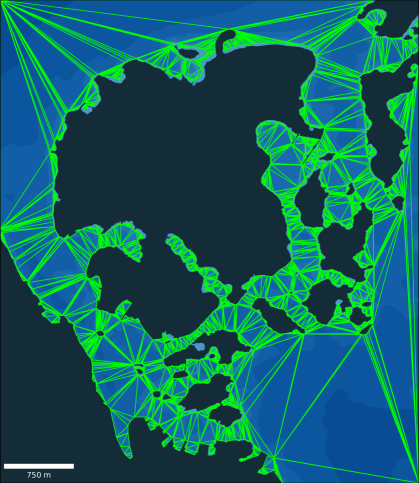
Figure 1: Constrained Delaunay Triangulation for a considered planning area near Stavanger, Norway. Triangles are shown with green edges, Land in dark blue, whereas the shore and seabed are shown in variations of brighter blue.

4.2 Data Structures

Another foundation of the RRT algorithms is nearest neighbor searches, used when wiring and re-wiring the tree for RRT*-variants. For spatial queries as is considered here, it is recommended to use R*-tree or R-tree-based data structures (Guttman, 1984; Beckmann et al., 1990) that are commonly used for storing spatial objects in e.g. databases. They have $O(log(n))$ complexity for insertion and distance-related queries for $n$ inserted elements. The trees are created such that leaf nodes of the tree hold spatial data, and parents or branching nodes correspond to the minimum bounding box that contains all of its children. With this structure, the R-tree utilizes data-based partitions into boxes of decreasing size as the tree grows. K-d trees have the same complexity as R-trees, and can also be used (Bentley, 1975). Note that the bonafide version is suitable only when the nodes are points and does not work well in high dimensions. Once polygons and other objects are introduced for representing the own-ship, static or dynamic hazards, standard k-d trees are also not compatible. The advantages of using R-trees are the efficient memory layout, tree update procedures and spatial nearest neighbor searching. For cases where the tree will not end up with a high number of objects or when few modifications and removals will be made on the go, it can on the other hand be sufficient to use k-d trees (Bentley, 1975).

These points also apply to the collision checking part, discussed below. Note that it might be worthwhile to consider a Mahalanobis distance metric when it is desired to evaluate the distance with respect to both position and other state variables such as orientation. In this regard, it will be wise to normalize the data before considering distance calculations.

4.3 Collision Checking

To accept a new node in the tree $\mathcal{T}$ maintained by the RRT algorithms, collision checks must be performed for each new trajectory segment $\bm{\sigma}_{new}$ resulting from the steering function in several parts of the RRT-algorithms. To ensure feasibility with respect to run-time, it is important to pre-process grounding hazard data using line simplification algorithms such as Ramer-Douglas-Peucker (Ramer, 1972) in order to reduce the map data accuracy to the required level. Especially for the maritime domain, one should merge multi polygons arising from hazardous land, shore and seabed objects as extracted from Electronic Navigation Charts (ENC) (Blindheim and Johansen, 2022), given the considered vessel and its draft. We recommend removing interior holes of land multi polygons arising from e.g. lakes, as these will naturally not be considered for sea voyages.

Again, it will also be important in this procedure to use efficient data structures such as R-trees for enabling fast distance computations in collision checking. Adherence to specified hazard clearance margins $d_{safe}$ can easily be done by buffering the hazard polygons before running the algorithm. Note that verification of sampled poses along a trajectory being collision-free is not exact, and operation in more confined space with smaller distance margins might require more accurate methods as in e.g. Zhang et al. (2022).

Note that collision checking requires significantly less effort when only two-point planar waypoint segments are considered, as opposed to a full trajectory segment with kinodynamical constraint consideration. This can be an option when the goal is to rapidly generate waypoints for a ship to follow, as opposed to a full trajectory to track. Some regard to maximum curvature based on the ship turn rate and speed should then be taken into account when accepting waypoint segments.

4.4 Steering

For trajectory planning RRTs, the steering functionality for connecting state pairs $(\bm{z}_{1},\bm{z}_{2})$ is a crucial part in the wiring of the tree, especially for non-holonomic systems. Previous methods have proposed e.g. the simplistic Dubin´s path for optimal steering (Karaman and Frazzoli, 2010), Bezier spline-based connectivity (Yang et al., 2014), learning-based steering and collision checking(Chiang et al., 2019), LQR-control-based extension (Perez et al., 2012) and lazy steering with a Neural Network (NN) for determining collision-free and steerable node extensions (Yavari et al., 2019). In this work, we apply LOS guidance for steering the ship towards new eligible nodes, as a low-cost solution for creating feasible trajectory segments in the maritime domain. One point that requires care in this context, is the early termination of the LOS guidance if the waypoint segment from $\bm{z}_{1}$ to a new node $\bm{z}_{2}$ is passed by, such that the computational cost of numerical integration of the ship dynamics is kept to a minimum. Further note that the integration time step should be increased in tact with the problem size, also related to the computational cost aspect.

5 Results

We present three cases in which the considered RRT-variants are compared. The first case demonstrates the usage of RRTs for rapid ship behavior generation, where the goal is to generate kinodynamically feasible trajectories for a specified ship scenario. The second case compares common RRT variants for a smaller planning scenario with a typical local minimum problem. Finally, the third case compares the RRT planners in a larger planning scenario. The framework in Tengesdal and Johansen (2023) is used as a platform for the simulation and utilization of Electronic Navigational Charts. The algorithms are implemented in the Rust programming language, and the executable is run on a MacBook Pro with an Apple Silicon M1 chip. We evaluate the obtained solutions with respect to run-time and trajectory lengths, over $N_{MC}=100$ Monte Carlo (MC) simulations for each case, where the RRTs are provided with different pseudorandom seeds on each run.

A kinematic model with parameters $T_{\chi}=$6\text{\,}\mathrm{s}$$, $T_{U}=$6\text{\,}\mathrm{s}$$, $r_{max}=$10\text{\,}\mathrm{\SIUnitSymbolDegree}\text{/}\mathrm{s}$$, $U_{min}=$0\text{\,}\mathrm{k}\mathrm{n}\mathrm{o}\mathrm{t}\mathrm{s}$$ and $U_{max}=$20\text{\,}\mathrm{k}\mathrm{n}\mathrm{o}\mathrm{t}\mathrm{s}$$ is considered for a ship with length about $15\text{\,}\mathrm{m}$, with LOS guidance parameters $\Delta=$30.0\text{\,}\mathrm{m}$$. The grounding hazards in the environment are buffered with a horizontal clearance parameter $d_{safe}$ of $0\text{\,}\mathrm{m}$ in the first two cases, and $5\text{\,}\mathrm{m}$ in the last case. This will in general be dependent on the map accuracy, application and ship type. We consider a time step $\delta_{sim}$ of $0.5\text{\,}\mathrm{s}$ in the first two cases, and $1.0\text{\,}\mathrm{s}$ in the last case, for the RRT kinematic ship model. For the RRTs we use R-trees to perform nearest neighbor searching and spatial queries, where grounding hazards (land, shore and relevant seabed) are extracted and merged considering a vessel draft of $1.0\text{\,}\mathrm{m}$. The merged hazards are then used to form a safe sea CDT, from which weighted samples are drawn.

Key parameters for the RRT-variants used in the first two cases are given in Table 1. For the first case, we did not find a configuration of PQ-RRT* parameters for the sample adjustment procedure that gave better result than just disabling the APF-based part as a whole, and thus used $N_{sa}^{max}=0$. All methods sample from the safe sea CDT using (12), except the IRRT* which uses (8) after a solution has been found. The PQ-RRT* will adjust the CDT sample using its goal potential field. We note that tuning of the RRT algorithms is non-trivial, and will be specific to the scale considered for the trajectory planning. This is a trade-off between both planner run-time, memory requirements, and solution quality. The number of iterations should be adequately high in order to increase the likelihood of the RRT finding a solution.

Table 1: Algorithm parameters for the smaller planning cases.

Parameter	PQ-RRT*	IRRT*	RRT*	RRT
$N_{node}^{max}$	$10000$	$10000$	$10000$	$10000$
$N_{iter}^{max}$	$25000$	$25000$	$25000$	$25000$
$\Delta_{goal}$	$500$	$500$	$500$	$500$
$d_{node}^{min}$	$5.0\text{\,}\mathrm{m}$	$5.0\text{\,}\mathrm{m}$	$5.0\text{\,}\mathrm{m}$	-
$\gamma$	$2000.0\text{\,}\mathrm{m}$	$2000.0\text{\,}\mathrm{m}$	$2000.0\text{\,}\mathrm{m}$	-
$T_{min}$	$1.0\text{\,}\mathrm{s}$	$1.0\text{\,}\mathrm{s}$	$1.0\text{\,}\mathrm{s}$	$1.0\text{\,}\mathrm{s}$
$T_{max}$	$30.0\text{\,}\mathrm{s}$	$30.0\text{\,}\mathrm{s}$	$30.0\text{\,}\mathrm{s}$	$30.0\text{\,}\mathrm{s}$
$R_{a}$	$20.0\text{\,}\mathrm{m}$	$20.0\text{\,}\mathrm{m}$	$20.0\text{\,}\mathrm{m}$	$20.0\text{\,}\mathrm{m}$
$\delta_{sim}$	$0.5\text{\,}\mathrm{s}$	$0.5\text{\,}\mathrm{s}$	$0.5\text{\,}\mathrm{s}$	$0.5\text{\,}\mathrm{s}$
$d_{margin}$	$0.1\text{\,}\mathrm{m}$	-	-	-
$N_{ancestry}$	$1$	-	-	-
$N_{sa}^{max}$	$0$	-	-	-
$\lambda_{sample}$	$1.0\text{\,}\mathrm{m}$	-	-	-

5.1 Random Vessel Trajectory Generation

The first case is a random vessel trajectory generation scenario where the goal is to generate multiple random trajectories from a given start position. After being built, the resulting RRT variant can be queried efficiently through R-tree spatial nearest neighbor search (Guttman, 1984), and used to rapidly sample random ship trajectories for intention-aware CAS or simulation-based testing of CAS. This is useful in the online setting for CAS, but also for interaction data generation to be used by learning-based CAS algorithms. Training of Reinforcement Learning (RL) agents with the Gymnasium framework typically require a reset of the environment after each terminated or truncated episode. In this context, RRT algorithms can be used for rapidly generating target ship trajectory scenarios after a reset. As an example, PQ-RRT* will, in general, produce more path-optimal solutions than RRT and RRT*, and can thus be used for spawning target ship behavior scenarios with minimal maneuvering, whereas the RRT* or RRT variants can be used for spawning gradually unpredictable maneuvering target ship behaviors that can be considered as outliers. Thus, employing multiple RRT algorithm variants for ship scenario generation can improve the ability of learning-based CAS to generalize, and also enlarge the test coverage in the context of simulation-based CAS verification.

Note that, in the scenario-generation context the RRT cost function can be designed to e.g. minimize time to collision or converge towards near misses between the random vessel and the own-ship that runs the CAS to be tested (Tuncali and Fainekos, 2019). Furthermore, in the maritime context, COLREG can be misinterpreted and lead to ambiguous and therefore often dangerous situations (Chauvin and Lardjane, 2008). Thus, RRTs could be guided towards edge case situations in COLREG where the applicable situation rule(s) are easy to misinterpret. These considerations are a topic for future work.

Fig. 2 shows an example of obstacle ship behavior generation for a CAS head-on situation. To make the figures less dense, we have reduced the maximum allowable tree nodes to $N_{node}^{max}=4000$ for all planners. In this particular case, we find built RRT, RRT*, and PQ-RRT* behaviors close to a randomly sampled position within a corridor given by the initial target ship position and course and its maximum travel length over the simulation timespan, i.e.

$$x_{corr} \sim\mathrm{Uniform}(x;-d_{corr}/2,d_{corr}/2)$$ (13)

$$y_{corr} \sim\mathrm{Uniform}(x;0,U_{d}^{os}T_{sim})$$

$$\alpha_{corr} =\textit{atan2}(y_{end}^{os}-y_{start}^{os},x_{end}^{os}-x_{start}^{os})$$

$$\bm{p}_{rand} =\bm{R}(\alpha_{corr})\begin{bmatrix}x_{corr}+x_{start}^{os}\\ y_{corr}+y_{start}^{os}\end{bmatrix},$$

with $d_{corr}$ as the corridor width parameter, $T_{sim}$ as the total simulation time-span, $U_{d}^{os}$ is the own-ship speed reference, and $(x_{start}^{os},y_{start}^{os})$ and $(x_{end}^{os},y_{end}^{os})$ are the own-ship start and end coordinates, respectively.

Fig 3 shows another case where we sample behaviors for a CAS crossing situation. In this situation, random position samples are drawn near the predicted closest point of approach (CPA) between the vessels, from which the nearest RRT behaviors or trajectories are fetched, i.e.

$$\bm{p}_{rand} =\mathrm{Normal}(\bm{p};\bm{p}_{cpa},\bm{\Sigma}),$$ (14)

where $\bm{p}_{cpa}$ is the target ship position at CPA, assuming constant speed and course for the two vessels, calculated as in e.g. Kuwata et al. (2014), and $\bm{\Sigma}$ the covariance parameter adjusting the spread of samples. This strategy allows for generating multiple target ship behaviors that will lead to a collision or near miss with the own-ship unless preventive actions are taken. The RRTs are flexible, and any of the navigational risk factors as outlined in Bolbot et al. (2022) could be considered as targets to develop sampling schemes from.

For each of the example situations, the behaviors parameterized by waypoints are shown sampled. Since the planners consider the underlying ship model dynamics, the waypoints will be feasible, in addition to being collision-free with respect to nearby static hazards. Note that we can also use the trajectory that accompanies the waypoints as well. Further note that we define a reduced-size bounding box considered by the RRT planners, in order to reduce computation time and consider only a subset of the grounding hazards present in the ENC. Once the RRTs are built, a new behavior can be sampled in less than $1\text{\,}\mathrm{m}\mathrm{s}$ on the considered computing platform, which makes the approach viable for large-scale scenario production. We also note that the trees can easily be built offline, and then effectively sampled from afterwards in the relevant context.

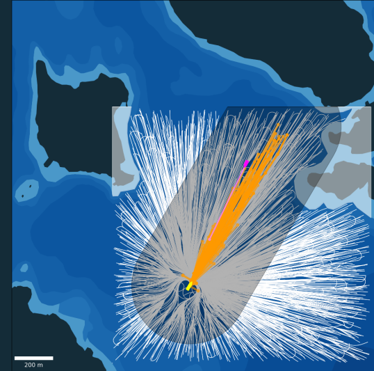
(a) PQ-RRT*.

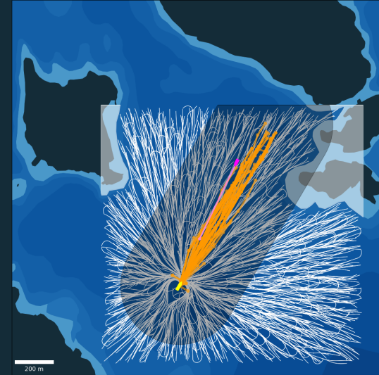
(b) RRT*.

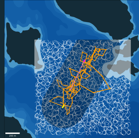
(c) RRT.

Figure 2: Results from random obstacle ship behavior generation for a CAS head-on situation near Halsnøya in Boknafjorden, Norway. The initial obstalcle ship position is shown in yellow, the initial own-ship position in pink and its waypoints in purple, the resulting tree in white, sampled obstacle ship behavior waypoint sequences in orange annuluses. The safety buffered hazard boundary are shown in red, with the planning bounding box shown in transparent white.

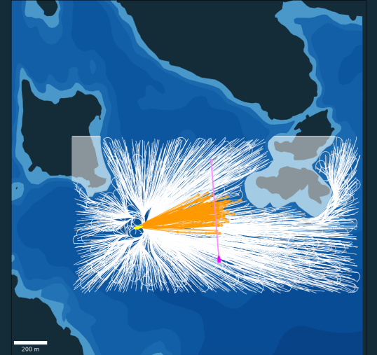
(a) PQ-RRT*.

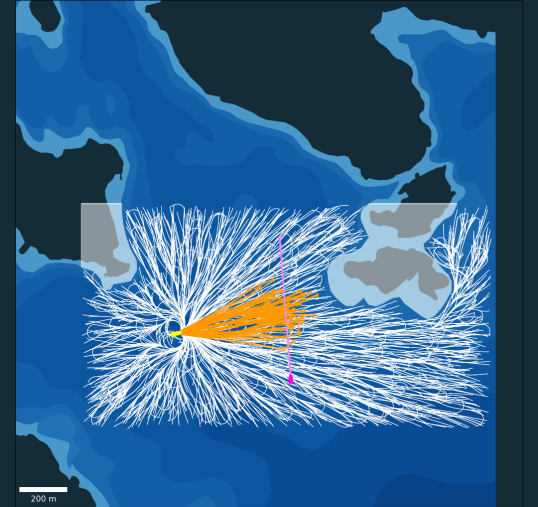
(b) RRT*.

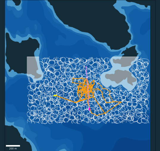
(c) RRT.

Figure 3: Results from random obstacle ship behavior generation for a CAS crossing situation near Børøy in Boknafjorden, Norway. The initial obstacle ship position is shown in yellow, the initial own-ship position in pink and its waypoints in purple, the resulting RRT in white, sampled obstacle ship behavior waypoint sequences in orange annuluses. The safety buffered hazard boundary are shown in red, with the planning bounding box shown in transparent white.

5.2 Smaller Planning Example

In the second case, we consider a smaller planning situation with a constant reference ship speed $U_{d}=$4.0\text{\,}\mathrm{m}\mathrm{/}\mathrm{s}$$, and allow the planners to find and refine their solution over the maximum allowable iterations and tree nodes up until a maximum time of $50\text{\,}\mathrm{s}$. The considered location near Kvitsøy in Rogaland, Norway has a map size of $$850\text{\,}\mathrm{m}$\times$750\text{\,}\mathrm{m}$$, and features a typical local minimum problem where one can get stuck in the dead end not far from the ship initial position. Note that as the planners sample from a CDT constructed from the safe sea area, the sampling efficiency will be higher, making it easier to avoid local minima issues.

Results from sample runs are shown in Figure 4, whereas solution statistics are given in Table 2. In the table, statistics for the time to find an initial solution $t_{sol,0}$ is reported, whereas run-time $t_{sol}$ and path length $d_{sol}$ statistics are reported for the final refined trajectory. The metric $\rho_{mc}$ is the success percentage of finding a solution out of all the MC runs. From Figure 4, it might look like there is a collision due to the orange waypoints crossing a hazard at some point. This is not the case, as the actual ship trajectories wired by the RRTs are collision-free, taking the nonholonomic properties of the ship into account.

The optimal solution has a path length of approximately $905\text{\,}\mathrm{m}$. Thus we see that the PQ-RRT*, IRRT* and RRT* are able to converge to within $6\%$ of the optimum. PQ-RRT* attains the best results with respect to path length, with a marginal difference to IRRT* and RRT*. On the other hand, the ancestor consideration in the tree rewiring plus extra functionality comes at the cost of higher runtimes. We also see a factor of 10 increase in the run-time between baseline RRT and RRT*, which is expected due to the more complicated wiring process.

For IRRT* we are able to get marginally better results than RRT*, at lower run-times. This is due to the high sample rejection rate after finding an initial solution, as samples are likely to be taken from $\mathcal{X}_{obst}$ in this map with large hazard coverage. However, accepted samples will have higher values, partially explaining the marginal improvement in solution lengths. Thus, it can here be a viable approach to iteratively prune out triangles in the safe sea CDT as the hyperellipsoid forming the sampling heuristic reduces in volume. One should thus implement efficient methods for re-computing the CDT from the new sampling domain, or for pruning CDT triangles outside the domain.

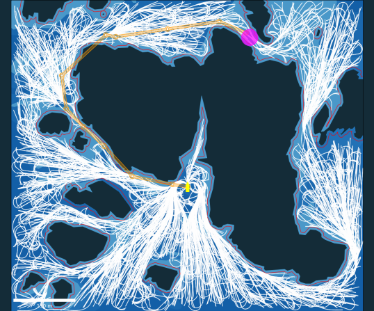
(a) PQ-RRT*.

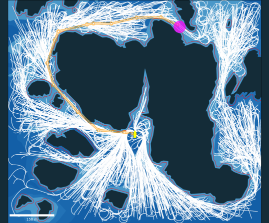
(b) IRRT*.

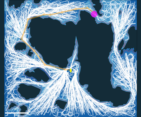
(c) RRT*.

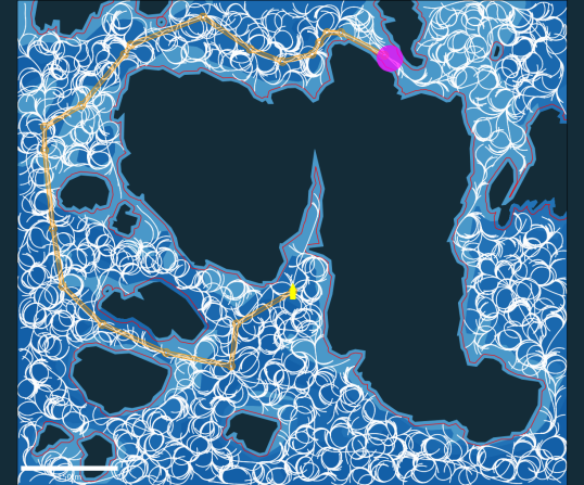
(d) RRT.

Figure 4: Results from the first MC sample run on the smaller planning case near Kvitsøy outside Stavanger, Norway. The starting ship pose is shown in yellow, the resulting tree in white, node waypoints in orange, and the goal in purple. The safety buffered hazard boundary is shown in red.

Table 2: Results for the smaller planning case over $N_{mc}=100$ MC runs.

Metric	PQ-RRT*	IRRT*	RRT*	RRT
$t_{sol,0}$	$5.5\pm$5.0\text{\,}\mathrm{s}$$	$3.5\pm$3.4\text{\,}\mathrm{s}$$	$2.9\pm$1.8\text{\,}\mathrm{s}$$	$0.14\pm$0.07\text{\,}\mathrm{s}$$
$(t_{sol,0}^{min},t_{sol,0}^{max})$	$($0.2\text{\,}\mathrm{s}$,$29.1\text{\,}\mathrm{s}$)$	$($0.2\text{\,}\mathrm{s}$,$15.4\text{\,}\mathrm{s}$)$	$($0.5\text{\,}\mathrm{s}$,$11.2\text{\,}\mathrm{s}$)$	$($0.03\text{\,}\mathrm{s}$,$0.45\text{\,}\mathrm{s}$)$
$t_{sol}$	$34.6\pm$2.5\text{\,}\mathrm{s}$$	$26.3\pm$0.7\text{\,}\mathrm{s}$$	$32.6\pm$0.5\text{\,}\mathrm{s}$$	$1.91\pm$0.03\text{\,}\mathrm{s}$$
$(t_{sol}^{min},t_{sol}^{max})$	$($28.8\text{\,}\mathrm{s}$,$38.9\text{\,}\mathrm{s}$)$	$($24.6\text{\,}\mathrm{s}$,$28.8\text{\,}\mathrm{s}$)$	$($31.5\text{\,}\mathrm{s}$,$34.1\text{\,}\mathrm{s}$)$	$($1.8\text{\,}\mathrm{s}$,$2.0\text{\,}\mathrm{s}$)$
$d_{sol}$	$963.1\pm$32.0\text{\,}\mathrm{m}$$	$965.9\pm$31.0\text{\,}\mathrm{m}$$	$968.3\pm$33.3\text{\,}\mathrm{m}$$	$1472.7\pm$163.7\text{\,}\mathrm{m}$$
$(d_{sol}^{min},d_{sol}^{max})$	$($914.0\text{\,}\mathrm{m}$,$1081.9\text{\,}\mathrm{m}$)$	$($920.0\text{\,}\mathrm{m}$,$1072.0\text{\,}\mathrm{m}$)$	$($909.9\text{\,}\mathrm{m}$,$1070.0\text{\,}\mathrm{m}$)$	$($1200.0\text{\,}\mathrm{m}$,$2013.8\text{\,}\mathrm{m}$)$
$\rho_{mc}$	$100\%$	$100\%$	$100\%$	$100\%$

5.3 Larger Planning Example

The larger planning example considers the region shown in Fig. 1 of size $$5.0\text{\,}\mathrm{k}\mathrm{m}$\times$5.0\text{\,}\mathrm{k}\mathrm{m}$$ with multiple islands and smaller grounding hazards, which increases the problem size substantially. Again, the planners are allowed to find and refine a solution over the maximum allowable iterations and nodes, up until a maximum time of $300\text{\,}\mathrm{s}$. A constant reference speed $U_{d}=$5.0\text{\,}\mathrm{m}\mathrm{/}\mathrm{s}$$ is utilized. In this case, due to the large map size, we utilize planner parameters as in Table 3.

Table 3: Algorithm parameters for the larger planning case.

Parameter	PQ-RRT*	Informed-RRT*	RRT*	RRT
$N_{node}^{max}$	$10000$	$10000$	$10000$	$10000$
$N_{iter}^{max}$	$25000$	$25000$	$25000$	$25000$
$\Delta_{goal}$	$500$	$500$	$500$	$500$
$d_{node}^{min}$	$15.0\text{\,}\mathrm{m}$	$15.0\text{\,}\mathrm{m}$	$15.0\text{\,}\mathrm{m}$	-
$\gamma$	$3500.0\text{\,}\mathrm{m}$	$3500.0\text{\,}\mathrm{m}$	$3500.0\text{\,}\mathrm{m}$	-
$T_{min}$	$1.0\text{\,}\mathrm{s}$	$1.0\text{\,}\mathrm{s}$	$1.0\text{\,}\mathrm{s}$	$1.0\text{\,}\mathrm{s}$
$T_{max}$	$30.0\text{\,}\mathrm{s}$	$30.0\text{\,}\mathrm{s}$	$30.0\text{\,}\mathrm{s}$	$30.0\text{\,}\mathrm{s}$
$R_{a}$	$20.0\text{\,}\mathrm{m}$	$20.0\text{\,}\mathrm{m}$	$20.0\text{\,}\mathrm{m}$	$20.0\text{\,}\mathrm{m}$
$\delta_{sim}$	$1.0\text{\,}\mathrm{s}$	$1.0\text{\,}\mathrm{s}$	$1.0\text{\,}\mathrm{s}$	$1.0\text{\,}\mathrm{s}$
$d_{margin}$	$0.5\text{\,}\mathrm{m}$	-	-	-
$N_{ancestry}$	$1$	-	-	-
$N_{sa}^{max}$	$50$	-	-	-
$\lambda_{sample}$	$8.0\text{\,}\mathrm{m}$	-	-	-

Visual results when applying the RRT-variants on the planning area in Fig. 1 are shown for sample runs in Fig. 5. Table 4 shows performance metrics for the algorithms over the MC runs. Again, we see a marginally better result for the PQ-RRT* than for IRRT* and RRT*. In this planning example, the IRRT* achieves worse results than RRT* due to the significantly higher sample rejection rate, again caused by a large obstacle congestion ratio, amplified by the problem scale.

The optimal solution is approximately $5.2\text{\,}\mathrm{k}\mathrm{m}$, and thus we see that the optimal algorithm variants only converges to within approximately $30\%$ of the optimum. The convergence issue is attributed to the map size and the optimal solution passes through narrow passages, as well as the complexity of also considering ship dynamics and kinodynamical constraints in the tree wiring and rewiring. A standard deviation of over $500\text{\,}\mathrm{m}$ is found for the path length solutions of all variants, which is significantly high.

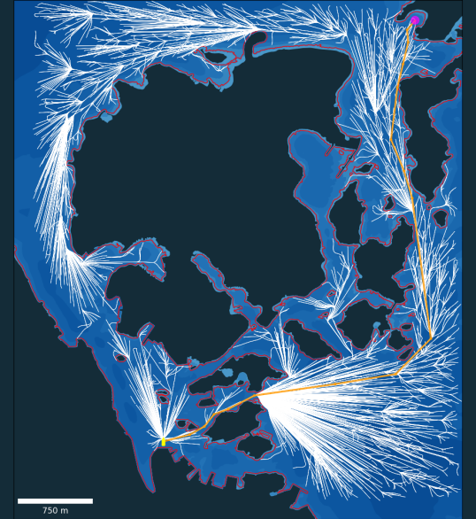
(a) PQ-RRT*.

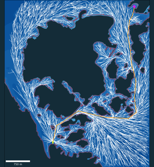
(b) IRRT*.

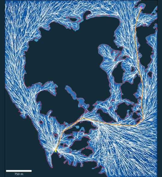
(c) RRT*.

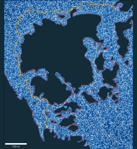
(d) RRT.

Figure 5: Results from the first MC sample run on the larger planning case near Vågen in Stavanger, Norway. The starting ship pose is shown in yellow, the resulting tree in white, node waypoints in orange, and the goal in purple. The safety buffered hazard boundary is shown in red.

Table 4: Results for the larger planning case over $N_{mc}=100$ MC runs.

Metric	PQ-RRT*	IRRT*	RRT*	RRT
$t_{sol,0}$	$62.7\pm$22.3\text{\,}\mathrm{s}$$	$60.7\pm$31.0\text{\,}\mathrm{s}$$	$60.7\pm$31.0\text{\,}\mathrm{s}$$	$3.8\pm$1.4\text{\,}\mathrm{s}$$
$(t_{sol,0}^{min},t_{sol,0}^{max})$	$($33.7\text{\,}\mathrm{s}$,$162.5\text{\,}\mathrm{s}$)$	$($19.0\text{\,}\mathrm{s}$,$205.0\text{\,}\mathrm{s}$)$	$($19.0\text{\,}\mathrm{s}$,$205.0\text{\,}\mathrm{s}$)$	$($1.6\text{\,}\mathrm{s}$,$9.6\text{\,}\mathrm{s}$)$
$t_{sol}$	$300.0\pm$0.0\text{\,}\mathrm{s}$$	$300.0\pm$0.0\text{\,}\mathrm{s}$$	$300.0\pm$0.0\text{\,}\mathrm{s}$$	$24.9\pm$2.1\text{\,}\mathrm{s}$$
$(t_{sol}^{min},t_{sol}^{max})$	$($300.0\text{\,}\mathrm{s}$,$300.0\text{\,}\mathrm{s}$)$	$($300.0\text{\,}\mathrm{s}$,$300.0\text{\,}\mathrm{s}$)$	$($300.0\text{\,}\mathrm{s}$,$300.0\text{\,}\mathrm{s}$)$	$($21.6\text{\,}\mathrm{s}$,$27.5\text{\,}\mathrm{s}$)$
$d_{sol}$	$6567.3\pm$407.7\text{\,}\mathrm{m}$$	$6836.6\pm$476.6\text{\,}\mathrm{m}$$	$6744.6\pm$487.4\text{\,}\mathrm{m}$$	$8805.3\pm$620.8\text{\,}\mathrm{m}$$
$(d_{sol}^{min},d_{sol}^{max})$	$($5239.9\text{\,}\mathrm{m}$,$7359.9\text{\,}\mathrm{m}$)$	$($5299.9\text{\,}\mathrm{m}$,$7534.9\text{\,}\mathrm{m}$)$	$($5269.9\text{\,}\mathrm{m}$,$7440.0\text{\,}\mathrm{m}$)$	$($6484.0\text{\,}\mathrm{m}$,$10\,178.5\text{\,}\mathrm{m}$)$
$\rho_{mc}$	$100\%$	$100\%$	$100\%$	$100\%$

5.4 Discussion

Gauging the results on planning, we see that the RRT-based planners are viable for use in problems of adequate size, i.e. less than $$1\text{\,}\mathrm{k}\mathrm{m}$\times$1\text{\,}\mathrm{k}\mathrm{m}$$ in map size. In these cases, the planners can find and optimize the best solution in adequate time. However, for larger maps, the planners struggle. This is attributed to the increased number of samples and iterations required in order to find and refine a solution. Although the planners find initial solutions very fast, they have a hard time optimizing the solutions when considering larger map sizes and complex unstructured environment. The run-time also increases substantially for larger problem sizes, due to the higher computational cost of re-wiring the tree and propagating new node costs to the leaves. Thus, in such large cases, it can be an option to utilize RRT-based planners without dynamics consideration, where the tree wiring only considers position sampling and the connection of these through collision-free straight-line segments. Alternatively, one can just use path complete algorithms such as A*, to find the solution fast up to a suitable grid resolution, without having randomness in the result. Note that it will then be necessary to post-process the solution in order to generate a feasible trajectory for a ship to track, e.g. Blindheim et al. (2023), unless a motion primitives-based planner is used.

We note that the IRRT*, although providing linear algorithm convergence properties for obstacle-free environments, struggles with both planning cases, but especially the larger one. This is due to the large volume occupied by obstacles in the configuration space, leading to a significant rejection rate in the informed heuristical sampling. Thus, for the IRRT* to be of practical usage, it requires an improvement. This can be an update and creation of a new CDT for the safe sea domain inside the informed sampling domain, each time a new solution is found.

For the PQ-RRT* with nonholonomic steering, we see a large increase in computational effort due to the ancestry consideration. This was viable for smaller planning cases, but proved to be more limiting in the larger case unless the nonholonomic steering functionality is disabled or higher simulation time steps are used. Also, the algorithm run-time and performance are highly dependent on the sample adjustment procedure, itself being dependent on the three parameters $N_{sa}^{max}$, $\lambda_{sa}$ and $d_{margin}$. In total, this leads to a lower tree node number and can in the worst cases prevent the algorithm from finding solutions. Choosing $\lambda_{sa}$ too small yields negligible gain from the APF-based adjustments, and requires a higher iteration number $N_{sa}^{max}$, which again gives higher algorithm run-time due to an increased number of obstacle distance calculations being required. Conversely, a large $\lambda_{sa}$ can lead to rapid convergence towards local minima. We found that a selection of $\lambda_{sa}$ in the order of $0.1\%$ of the map width, and an adjustment number of around $N_{sa}^{max}\approx 50$ gave a reasonable trade-off between run-time and solution quality for the larger planning case in this work. For the clearance parameter $d_{margin}$ it was found necessary to select a smaller value of around $0.5\text{\,}\mathrm{m}$, as a high value can prevent the planner from wiring into more confined areas. Because of these factors, we found the tuning of PQ-RRT* to be significantly more challenging than the other variants. Judging from the marginal improvements found in this work with consideration of nonholonomic steering, we argue that it was easier to employ IRRT* or RRT*, which required less tuning effort and achieved comparable performance. In general, we note that the parameter selection is dependent on the vehicle steering system. Another tuning challenge is the selection of $\gamma$, also mentioned in Noreen et al. (2016a), which has a large influence on performance. As the ball volume reduces with the tree size, too small values of $\gamma$ can lead to negligible search radius and can in the worst case effectively reduce optimal RRT variants to the baseline RRT, where no nearest neighbors other than the closest one are considered in the wiring. A solution to consider is to bound the search radius from below, or for simplicity consider a fixed search radius.

We see that the common challenge of RRTs, related to a slow convergence rate towards the optimum, are increasing when applying the algorithms to large unstructured environments. This is partially due to the sampling inefficiency and node rejection rate issue found in most variants, and for which a significant amount of solutions have been proposed in Véras et al. (2019) with varying level of success. Also, for real-time systems and applications where time is a resource, the incremental tree wiring and re-wiring induces a computational cost that must be weighted against performance and optimality. As such, and also considering the results of this work, we deem computationally constrained RRT planners without sophisticated sampling strategies and without coupling to graph-search-based methods such as A*, to be more suitable for smaller problems, or problems where obstacles occupy a smaller portion of the configuration space, or where non-optimal solutions are acceptable. For planning in higher dimensional space, it is also necessary to consider other metrics than the Euclidean one (Noreen et al., 2016a).

6 Conclusion

In this article, multiple algorithms for ship trajectory planning based on RRT have been developed and compared with respect to path length and computational time. The comparison focuses on varying degrees of difficulty in an unstructured environment. Practical aspects to consider when employing such algorithms in the maritime domain are also outlined and discussed, to the benefit of researchers and practitioners in the field. It is also shown through an example case that RRT variants can be beneficial in the context of automatic test scenario generation, where target ship trajectories can be sampled efficiently directly from the nodes of a built RRT. The tree can alternatively be used to sample intention scenarios for use in intelligent CAS.

From Monte Carlo simulations on selected cases, we see that PQ-RRT* attains more distance optimal trajectories, with IRRT* and RRT* following close behind, naturally at the cost of increased run-time due to its nearest neighbor searches and consideration in both wiring and rewiring. IRRT* struggles with cases where obstacles cover a large part of the configuration space. In larger planning cases there is a need for more efficient sampling procedures in order for optimal RRT* variants to be viable, due to the significant space of configurations that must be covered, causing a similar curse of dimensionality issue. This causes inefficiencies in the trade-off between computational effort, available memory and performance, as the optimal variants will then spend the majority of their effort wiring and re-wiring its tree.

From the results and through tuning of the algorithm, it was found that the PQ-RRT* involves much higher complexity in tuning than the other variants, because of the sample adjustment procedure and ancestor consideration. On the other hand, the IRRT* algorithm here attains a good balance between simpler tuning and obtainable performance. Its informed sampling heuristic should, however, be improved to reduce its sample rejection rate. In the maritime domain, this can be achieved by an iterative pruning or update of a safe sea triangulation used to sample new collision-free configurations.

References

- Beckmann et al. (1990) Beckmann, N., Kriegel, H.P., Schneider, R., Seeger, B., 1990. The r*-tree: An efficient and robust access method for points and rectangles, in: Proceedings of the 1990 ACM SIGMOD international conference on Management of data, pp. 322–331.
- Bentley (1975) Bentley, J.L., 1975. Multidimensional binary search trees used for associative searching. Communications of the ACM 18, 509–517.
- Blindheim and Johansen (2022) Blindheim, S., Johansen, T.A., 2022. Electronic navigational charts for visualization, simulation, and autonomous ship control. IEEE Access 10, 3716–3737. doi:10.1109/ACCESS.2021.3139767.
- Blindheim et al. (2023) Blindheim, S., Rokseth, B., Johansen, T.A., 2023. Autonomous machinery management for supervisory risk control using particle swarm optimization. J. Marine Science and Engineering 11.
- Bolbot et al. (2022) Bolbot, V., Gkerekos, C., Theotokatos, G., Boulougouris, E., 2022. Automatic traffic scenarios generation for autonomous ships collision avoidance system testing. Ocean Engineering 254, 111309.
- Breivik and Fossen (2008) Breivik, M., Fossen, T.I., 2008. Guidance laws for planar motion control, in: Proc. 47th IEEE Conf. Decision and Control, pp. 570–577. doi:10.1109/CDC.2008.4739465.
- Chauvin and Lardjane (2008) Chauvin, C., Lardjane, S., 2008. Decision making and strategies in an interaction situation: Collision avoidance at sea. Transportation Research Part F: Traffic Psychology and Behaviour 11, 259–269.
- Chiang and Tapia (2018) Chiang, H.L., Tapia, L., 2018. COLREG-RRT: An RRT-based COLREGS-compliant motion planner for surface vehicle navigation. IEEE Robotics and Automation Letters 3, 2024–2031. doi:10.1109/LRA.2018.2801881.
- Chiang et al. (2019) Chiang, H.T.L., Hsu, J., Fiser, M., Tapia, L., Faust, A., 2019. Rl-rrt: Kinodynamic motion planning via learning reachability estimators from rl policies. IEEE Robotics and Automation Letters 4, 4298–4305. doi:10.1109/LRA.2019.2931199.
- Dang et al. (2008) Dang, T., Donze, A., Maler, O., Shalev, N., 2008. Sensitive state-space exploration, in: 2008 47th IEEE Conference on Decision and Control, pp. 4049–4054. doi:10.1109/CDC.2008.4739371.
- Enevoldsen et al. (2022) Enevoldsen, T.T., Blanke, M., Galeazzi, R., 2022. Sampling-based collision and grounding avoidance for marine crafts. Ocean Engineering 261, 112078.
- Enevoldsen et al. (2021) Enevoldsen, T.T., Reinartz, C., Galeazzi, R., 2021. Colregs-informed rrt* for collision avoidance of marine crafts, in: 2021 IEEE International Conference on Robotics and Automation (ICRA), IEEE. pp. 8083–8089.
- Gammell et al. (2014) Gammell, J.D., Srinivasa, S.S., Barfoot, T.D., 2014. Informed rrt: Optimal sampling-based path planning focused via direct sampling of an admissible ellipsoidal heuristic, in: 2014 IEEE/RSJ International Conference on Intelligent Robots and Systems, IEEE. pp. 2997–3004.
- Guttman (1984) Guttman, A., 1984. R-trees: A dynamic index structure for spatial searching, in: Proceedings of the 1984 ACM SIGMOD international conference on Management of data, pp. 47–57.
- Hart et al. (1968) Hart, P.E., Nilsson, N.J., Raphael, B., 1968. A formal basis for the heuristic determination of minimum cost paths. IEEE transactions on Systems Science and Cybernetics 4, 100–107.
- Huang et al. (2020) Huang, Y., Chen, L., Chen, P., Negenborn, R.R., van Gelder, P., 2020. Ship collision avoidance methods: State-of-the-art. Safety Science 121, 451–473.
- IMO (2003) IMO, C., 2003. Convention on the International Regulations for Preventing Collisions at SEA, 1972.
- Jeong et al. (2019) Jeong, I.B., Lee, S.J., Kim, J.H., 2019. Quick-rrt*: Triangular inequality-based implementation of rrt* with improved initial solution and convergence rate. Expert Systems with Applications 123, 82–90.
- Karaman and Frazzoli (2010) Karaman, S., Frazzoli, E., 2010. Optimal kinodynamic motion planning using incremental sampling-based methods, in: 49th IEEE Conference on Decision and Control (CDC), pp. 7681–7687. doi:10.1109/CDC.2010.5717430.
- Karaman et al. (2011) Karaman, S., Walter, M.R., Perez, A., Frazzoli, E., Teller, S., 2011. Anytime motion planning using the rrt*, in: 2011 IEEE International Conference on Robotics and Automation, pp. 1478–1483. doi:10.1109/ICRA.2011.5980479.
- Kavraki et al. (1996) Kavraki, L.E., Svestka, P., Latombe, J.C., Overmars, M.H., 1996. Probabilistic roadmaps for path planning in high-dimensional configuration spaces. IEEE transactions on Robotics and Automation 12, 566–580.
- Klemm et al. (2015) Klemm, S., Oberländer, J., Hermann, A., Roennau, A., Schamm, T., Zollner, J.M., Dillmann, R., 2015. Rrt*-connect: Faster, asymptotically optimal motion planning, in: 2015 IEEE international conference on robotics and biomimetics (ROBIO), IEEE. pp. 1670–1677.
- Koschi et al. (2019) Koschi, M., Pek, C., Maierhofer, S., Althoff, M., 2019. Computationally efficient safety falsification of adaptive cruise control systems, in: 2019 IEEE Intelligent Transportation Systems Conference (ITSC), pp. 2879–2886. doi:10.1109/ITSC.2019.8917287.
- Kuwata et al. (2014) Kuwata, Y., Wolf, M.T., Zarzhitsky, D., Huntsberger, T.L., 2014. Safe maritime autonomous navigation with COLREGS, using velocity obstacles. IEEE Journal of Oceanic Engineering 39, 110–119. doi:10.1109/JOE.2013.2254214.
- Lai et al. (2019) Lai, T., Ramos, F., Francis, G., 2019. Balancing global exploration and local-connectivity exploitation with rapidly-exploring random disjointed-trees, in: 2019 International Conference on Robotics and Automation (ICRA), pp. 5537–5543. doi:10.1109/ICRA.2019.8793618.
- LaValle et al. (1998) LaValle, S.M., et al., 1998. Rapidly-exploring random trees: A new tool for path planning .
- Li et al. (2020) Li, Y., Wei, W., Gao, Y., Wang, D., Fan, Z., 2020. Pq-rrt*: An improved path planning algorithm for mobile robots. Expert systems with applications 152, 113425.
- Lindemann and LaValle (2004) Lindemann, S., LaValle, S., 2004. Incrementally reducing dispersion by increasing voronoi bias in rrts, in: IEEE International Conference on Robotics and Automation, 2004. Proceedings. ICRA ’04. 2004, pp. 3251–3257 Vol.4. doi:10.1109/ROBOT.2004.1308755.
- Minne (2017) Minne, P.K.E., 2017. Automatic testing of maritime collision avoidance algorithms. Master’s thesis. NTNU.
- Nasir et al. (2013) Nasir, J., Islam, F., Malik, U., Ayaz, Y., Hasan, O., Khan, M., Muhammad, M.S., 2013. Rrt*-smart: A rapid convergence implementation of rrt*. International Journal of Advanced Robotic Systems 10, 299. doi:10.5772/56718.
- Noreen et al. (2016a) Noreen, I., Khan, A., Habib, Z., 2016a. A comparison of rrt, rrt* and rrt*-smart path planning algorithms. International Journal of Computer Science and Network Security (IJCSNS) 16, 20.
- Noreen et al. (2016b) Noreen, I., Khan, A., Habib, Z., 2016b. Optimal path planning using rrt* based approaches: a survey and future directions. International Journal of Advanced Computer Science and Applications 7.
- Pedersen et al. (2020) Pedersen, T.A., Glomsrud, J.A., Ruud, E.L., Simonsen, A., Sandrib, J., Eriksen, B.O.H., 2020. Towards simulation-based verification of autonomous navigation systems. Safety Science 129, 104799.
- Pedersen et al. (2022) Pedersen, T.A., Åse Neverlien, Glomsrud, J.A., Ibrahim, I., Mo, S.M., Rindarøy, M., Torben, T., Rokseth, B., 2022. Evolution of safety in marine systems: From system-theoretic process analysis to automated test scenario generation. Journal of Physics: Conference Series 2311, 012016. doi:10.1088/1742-6596/2311/1/012016.
- Perez et al. (2012) Perez, A., Platt, R., Konidaris, G., Kaelbling, L., Lozano-Perez, T., 2012. Lqr-rrt*: Optimal sampling-based motion planning with automatically derived extension heuristics, in: 2012 IEEE International Conference on Robotics and Automation, IEEE. pp. 2537–2542.
- Porres et al. (2020) Porres, I., Azimi, S., Lilius, J., 2020. Scenario-based testing of a ship collision avoidance system, in: 2020 46th Euromicro Conference on Software Engineering and Advanced Applications (SEAA), pp. 545–552. doi:10.1109/SEAA51224.2020.00090.
- Qureshi and Ayaz (2016) Qureshi, A.H., Ayaz, Y., 2016. Potential functions based sampling heuristic for optimal path planning. Autonomous Robots 40, 1079–1093.
- Ramer (1972) Ramer, U., 1972. An iterative procedure for the polygonal approximation of plane curves. Computer Graphics and Image Processing 1, 244–256.
- Tengesdal and Johansen (2023) Tengesdal, T., Johansen, T.A., 2023. Simulation framework and software environment for evaluating automatic ship collision avoidance algorithms*, in: 2023 IEEE Conference on Control Technology and Applications (CCTA), pp. 186–193. doi:10.1109/CCTA54093.2023.10252863.
- Tengesdal et al. (2022) Tengesdal, T., Johansen, T.A., Grande, T.D., Blindheim, S., 2022. Ship collision avoidance and anti grounding using parallelized cost evaluation in probabilistic scenario-based model predictive control. IEEE Access 10, 111650–111664. doi:10.1109/ACCESS.2022.3215654.
- Tengesdal et al. (2023) Tengesdal, T., Rothmund, S.V., Basso, E.A., Johansen, T.A., Schmidt-Didlaukies, H., 2023. Obstacle intention awareness in automatic collision avoidance: Full scale experiments in confined waters. Field Robotics In press.
- Torben et al. (2022) Torben, T.R., Glomsrud, J.A., Pedersen, T.A., Utne, I.B., Sørensen, A.J., 2022. Automatic simulation-based testing of autonomous ships using gaussian processes and temporal logic. Proceedings of the Institution of Mechanical Engineers, Part O: Journal of Risk and Reliability 0. doi:10.1177/1748006X211069277.
- Tuncali and Fainekos (2019) Tuncali, C.E., Fainekos, G., 2019. Rapidly-exploring random trees for testing automated vehicles, in: 2019 IEEE Intelligent Transportation Systems Conference (ITSC), pp. 661–666. doi:10.1109/ITSC.2019.8917375.
- Vagale et al. (2021) Vagale, A., Bye, R.T., Oucheikh, R., Osen, O.L., Fossen, T.I., 2021. Path planning and collision avoidance for autonomous surface vehicles ii: a comparative study of algorithms. Journal of Marine Science and Technology doi:10.1007/s00773-020-00790-x.
- Véras et al. (2019) Véras, L.G.D., Medeiros, F.L., Guimaráes, L.N., 2019. Systematic literature review of sampling process in rapidly-exploring random trees. IEEE Access 7, 50933–50953.
- Wang et al. (2020) Wang, J., Chi, W., Li, C., Wang, C., Meng, M.Q.H., 2020. Neural rrt*: Learning-based optimal path planning. IEEE Transactions on Automation Science and Engineering 17, 1748–1758. doi:10.1109/TASE.2020.2976560.
- Yang et al. (2014) Yang, K., Moon, S., Yoo, S., Kang, J., Doh, N.L., Kim, H.B., Joo, S., 2014. Spline-based rrt path planner for non-holonomic robots. Journal of Intelligent & Robotic Systems 73, 763–782.
- Yavari et al. (2019) Yavari, M., Gupta, K., Mehrandezh, M., 2019. Lazy steering rrt*: An optimal constrained kinodynamic neural network based planner with no in-exploration steering, in: 2019 19th International Conference on Advanced Robotics (ICAR), pp. 400–407. doi:10.1109/ICAR46387.2019.8981551.
- Zhang et al. (2022) Zhang, Z., Zhang, Y., Han, R., Zhang, L., Pan, J., 2022. A generalized continuous collision detection framework of polynomial trajectory for mobile robots in cluttered environments. IEEE Robotics and Automation Letters 7, 9810–9817. doi:10.1109/LRA.2022.3191934.
- Zhu et al. (2022) Zhu, F., Zhou, Z., Lu, H., 2022. Randomly testing an autonomous collision avoidance system with real-world ship encounter scenario from ais data. Journal of Marine Science and Engineering 10. doi:10.3390/jmse10111588.