Extrapolated Plug-and-Play Three-Operator Splitting Methods for Nonconvex Optimization with Applications to Image Restoration

Abstract

This paper investigates the convergence properties and applications of the three-operator splitting method, also known as Davis-Yin splitting (DYS) method, integrated with extrapolation and Plug-and-Play (PnP) denoiser within a nonconvex framework. We first propose an extrapolated DYS method to effectively solve a class of structural nonconvex optimization problems that involve minimizing the sum of three possible nonconvex functions. Our approach provides an algorithmic framework that encompasses both extrapolated forward-backward splitting and extrapolated Douglas-Rachford splitting methods. To establish the convergence of the proposed method, we rigorously analyze its behavior based on the Kurdyka-Łojasiewicz property, subject to some tight parameter conditions. Moreover, we introduce two extrapolated PnP-DYS methods with convergence guarantee, where the traditional regularization prior is replaced by a gradient step-based denoiser. This denoiser is designed using a differentiable neural network and can be reformulated as the proximal operator of a specific nonconvex functional. We conduct extensive experiments on image deblurring and image super-resolution problems, where our results showcase the advantage of the extrapolation strategy and the superior performance of the learning-based model that incorporates the PnP denoiser in terms of achieving high-quality recovery images.

90C26, 90C30, 90C90, 65K05

1 Introduction

In this paper, we consider the following type of structural nonconvex optimization problem:

(1) $$\min_{{\bf x}\in\mathbb{R}^{n}}F({\bf x})=f_{1}({\bf x})+f_{2}({\bf x})+h({\bf x}),$$

where $f_{1}$ and $h$ are continuously differentiable and potentially nonconvex, and $f_{2}$ is a proper closed (possibly nonconvex) function. The model Eq. 1 captures a rich number of applications in fields of deep learning, signal and image processing, and statistical learning, see e.g., [7, 14, 15, 29, 74, 75, 76]. In particular, the smooth term includes the least squares or logistic loss functions, and the nonsmooth term can be represented as regularizers, e.g., to promote potential behavior such as sparsity and low-rank.

Splitting methods, which fully leverage the inherent separable structure, is a class of popular and state-of-the-art approaches for effectively addressing structural optimization problems. A generic way to solve the type of problem Eq. 1 is the three-operator splitting method, also known as Davis-Yin splitting (DYS) method which was first studied in [16] for convex optimization, i.e., all the involved functions in Eq. 1 are convex. The concrete iterative scheme of DYS method can be read as

(2) $$\left\{\begin{array}[]{l}{\bf y}^{k+1}\in\operatorname*{arg\,min}\limits_{{\bf y}\in\mathbb{R}^{n}}\left\{f_{1}({\bf y})+\frac{1}{2\gamma}\left\|{\bf y}-{\bf x}^{k}\right\|^{2}\right\},\\[8.5359pt] {\bf z}^{k+1}\in\operatorname*{arg\,min}\limits_{{\bf z}\in\mathbb{R}^{n}}\left\{f_{2}({\bf z})+\frac{1}{2\gamma}\left\|{\bf z}-\left(2{\bf y}^{k+1}-\gamma\nabla h\left({\bf y}^{k+1}\right)-{\bf x}^{k}\right)\right\|^{2}\right\},\\[8.5359pt] {\bf x}^{k+1}={\bf x}^{k}+\left({\bf z}^{k+1}-{\bf y}^{k+1}\right),\end{array}\right.$$

where $\gamma>0$ is a proximal parameter. DYS method Eq. 2 includes two proximal subproblems with respect to ${\bf y}$ and ${\bf z}$, which extends various previous splitting schemes such as the forward-backward splitting (FBS) method [3], Douglas-Rachford splitting (DRS) method [34], alternating direction method of multipliers (ADMM) algorithm [23] and the generalized forward-backward splitting method [51]. Later on, some variants and extensions of DYS method are explored for convex optimization [32, 56, 57, 62]. However, for the nonconvex setting as that in Eq. 1, convergence properties of the DYS method Eq. 2 are less understood. In contrast, the FBS method and DRS method, two special cases of the DYS method, have been well studied for nonconvex optimization, see e.g., [3, 34, 63]. Indeed, splitting methods are widely employed in image processing because numerous problems in image restoration can be addressed through variational methods. The resulting image is obtained as a minimizer of a suitable energy functional, typically exhibiting a separable structure. For recent applications in this field, we refer to [17, 40, 58, 62].

Another captivating and intriguing topic within the realm of splitting methods is the incorporation of acceleration techniques. Since the pioneering work of Polyak [50] on the heavy-ball method approach to gradient descent, extrapolation, as well as named inertial strategy, has been adapted to various optimization schemes to achieve accelerated convergence. Notable examples include the accelerated proximal point algorithm [12] for variational inequality problems and the accelerated FBS [4, 68, 6] for convex optimization. Over the past decade, the extrapolation technique has also been extended to various splitting methods for solving nonconvex optimization problems and expediting convergence based on Kurdyka–Łojasiewicz framework (see Definition 2.2), as demonstrated in studies such as [45, 33, 69, 37, 49, 73, 72, 48]. In this paper, our first focus is to investigate the convergence properties of the DYS method Eq. 2 when combined with extrapolation technique for solving Eq. 1. This endeavor will result in the development of a versatile framework encompassing extrapolated (or named inertial) FBS and extrapolated DRS methods as specialized schemes tailored for nonconvex optimization.

Recently, Plug-and-Play (PnP) methods combine splitting algorithm with denoising priors are widely used in solving many practical problems [19, 70, 71, 35]. PnP method offers a concise yet adaptable approach for integrating statistical priors into a problem, eliminating the requirement to explicitly construct an objective function. The first PnP method was the PnP-ADMM developed in [67] to address a range of imaging problems, which simply replaces the proximal subproblem with the denoising prior. Since then, many PnP-based methods such as PnP-FBS [59, 66], PnP-DRS [10, 28] and PnP-primal dual [46] approaches, reported empirical success on a large variety of applications, but with scarce theoretical guarantees. In several recent studies, the convergence of PnP methods has been achieved through the utilization of contractive fixed-point iterations. For example, the convergence of various proximal algorithms has been established by assuming properties such as denoiser averaging [60], firm nonexpansiveness [61], or simple nonexpansiveness [41, 52]. However, it is important to note that off-the-shelf deep denoisers often lack 1-Lipschitz continuity, which is equivalent to nonexpansiveness. The imposition of strict Lipschitz constraints on the network adversely affects its denoising performance [24, 28].

To address the challenge of nonexpansiveness in deep denoisers, Ryu et al. [55] proposed a method where each layer is individually normalized using its spectral norm. However, this approach imposes limitations on the utilization of residual skip connections, which are widely employed in deep denoisers. In a recent study, Hurault et al. [27] tackled this issue by training a deep image denoiser using a gradient-based PnP prior. By replacing the regularization step with the constructed denoiser, they demonstrated that the resulting gradient step PnP prior corresponds to the proximal operator of a specific nonconvex functional [28]. Under this condition, they successfully established the convergence of PnP-FBS, PnP-ADMM, and PnP-DRS iterates towards stationary points of explicit functions. Inspired by this research direction, it is worth exploring the convergence guarantees and potential applications of combining PnP methods with the DYS algorithm Eq. 2 in the form of Eq. 1.

1.1 Our contribution

This paper provides a generic algorithm framework that combines splitting methods, extrapolation strategy, and deep prior. The main contributions of this paper are threefold:

• We propose an extrapolated DYS method for solving the type of structural nonconvex optimization problem Eq. 1, which provides a generic algorithm framework including extrapolated FBS and extrapolated DRS methods. Under the tight parameter conditions, the convergence of the generated iterates is established based on Kurdyka–Łojasiewicz framework.

• By replacing the regularization step with the gradient step-based denoiser, we propose two extrapolated PnP-DYS methods. The denoiser is constructed by a differentiable neural network and can be reformulated as the proximal operator of a specific nonconvex functional. The convergence of both PnP-DYS algorithms is also established.

• Extensive experiments on image deblurring and image super-resolution problems are conducted to evaluate the performance of the proposed schemes. The numerical results illustrate the advantages and efficiency of the extrapolation strategy. Moreover, the experiments reveal the superiority of the PnP-based model with deep denoiser in terms of the quality of the recovered images.

1.2 Organization

The remainder of this paper is organized as follows. Some related methods and preliminaries are reviewed in Section 2. An extrapolated DYS method with convergence analysis is developed in Section 3. Section 4 combines PnP approach and produces two extrapolated PnP-DYS methods with convergence guarantee. Some experimental results are reported in Section 5, and the conclusions follow in Section 6.

1.3 Notation

We use $\mathbb{R}^{n}$ to denote the $n$-dimensional Euclidean space, $\mathbb{R}_{+}$ to denote the set of nonnegative real numbers, $\langle\cdot,\cdot\rangle$ to denote the inner product, and $\|\cdot\|$ to denote the norm induced from the inner product. For an extended real-valued function $f$, the domain of $f$ is defined as ${\rm dom}f:=\{{\bf x}\in\mathbb{R}^{n}\;|\;f({\bf x})<\infty\}$. We say that the function $f$ is proper if ${\rm dom}f\neq\emptyset$ and $f({\bf x})>-\infty$ for any ${\bf x}\in{\rm dom}f$, and is closed if it is lower semicontinuous. For any subset $S\subseteq\mathbb{R}^{n}$ and any point ${\bf x}\in\mathbb{R}^{n}$, the distance from ${\bf x}$ to $S$ is defined by ${\rm dist}({\bf x},S):=\inf\left\{\|{\bf y}-{\bf x}\|\;\big{|}\;{\bf y}\in S\right\},$ and ${\rm dist}({\bf x},S)=\infty$ for all $\bf x$ when $S=\emptyset$.

2 Preliminaries

In this section, we review the definitions of subdifferential and Kurdyka-Łojasiewicz (KL) property for further analysis.

Definition 2.1.

[3, 8] (Subdifferentials) Let $f:\mathbb{R}^{n}\rightarrow(-\infty,+\infty]$ be a proper and lower semicontinuous function.

• For a given ${\bf x}\in{\rm dom}f$, the Fréchet subdifferential of $f$ at ${\bf x}$, written by $\widehat{\partial}f({\bf x})$, is the set of all vectors ${\bf u}\in\mathbb{R}^{n}$ satisfying

  $$\liminf_{{\bf y}\neq{\bf x},{\bf y}\rightarrow{\bf x}}\frac{f({\bf y})-f({\bf x})-\langle{\bf u},{\bf y}-{\bf x}\rangle}{\|{\bf y}-{\bf x}\|}\geq 0,\vspace{-0.05in}$$

  and we set $\widehat{\partial}f({\bf x})=\emptyset$ when ${\bf x}\notin{\rm dom}f$.

• The limiting-subdifferential, or simply the subdifferential, of $f$ at ${\bf x}$, written by $\partial f({\bf x})$, is defined by

  (3) $$\partial f({\bf x}):=\{{\bf u}\in\mathbb{R}^{n}\;|\;\exists~{}{\bf x}^{k}\rightarrow{\bf x},~{}{\rm s.t.}~{}f({\bf x}^{k})\rightarrow f({\bf x})~{}{\rm and}~{}\widehat{\partial}f({\bf x}^{k})\ni{\bf u}^{k}\rightarrow{\bf u}\}.$$

• A point ${\bf x}^{*}$ is called (limiting-)critical point or stationary point of $f$ if it satisfies $0\in\partial f({\bf x}^{*})$, and the set of critical points of $f$ is denoted by ${\rm crit}f$.

Definition 2.1 implies that the property $\widehat{\partial}f({\bf x})\subseteq\partial f({\bf x})$ holds immediately, and $\widehat{\partial}f({\bf x})$ is closed and convex while $\partial f({\bf x})$ is closed. Indeed, the subdifferential Eq. 3 reduces to the gradient of $f$ denoted by $\nabla f$ if $f$ is continuously differentiable. Furthermore, as described in [53], if $g$ is a continuously differentiable function, it holds that $\partial(f+g)=\partial f+\nabla g$.

Next, we recall the KL property [2, 8], which is important in the convergence analysis.

Definition 2.2.

(KL property and KL function) Let $f:\mathbb{R}^{n}\rightarrow(-\infty,+\infty]$ be a proper and lower semicontinuous function.

• The function $f$ is said to have KL property at ${\bf x}^{*}\in{\rm dom}(\partial f)$ if there exist $\eta\in(0,+\infty]$, a neighborhood $U$ of ${\bf x}^{*}$ and a continuous and concave function $\varphi:[0,\eta)\rightarrow\mathbb{R}_{+}$ such that

  • $\varphi(0)=0$ and $\varphi$ is continuously differentiable on $(0,\eta)$ with $\varphi^{\prime}>0$;

  • for all ${\bf x}\in U\cap\{{\bf z}\in\mathbb{R}^{n}\;|\;f({\bf x}^{*})<f({\bf z})<f({\bf x}^{*})+\eta\}$, the following KL inequality holds:

    (4) $$\varphi^{\prime}(f({\bf x})-f({\bf x}^{*})){\rm dist}(0,\partial f({\bf x}))\geq 1.$$

• If $f$ satisfies the KL property at each point of dom$(\partial f)$, then $f$ is called a KL function.

Denote $\Phi_{\eta}$ as the set of functions $\varphi$ which satisfy the involved conditions in Definition 2.2(a). Then, we give an uniformized KL property which was established in [8] in the following, it will be useful for further convergence analysis.

Lemma 2.3.

[8] (Uniformized KL property) Let $f:\mathbb{R}^{n}\rightarrow(-\infty,+\infty]$ be a proper and lower semicontinuous function and $\Omega$ be a compact set. Assume that $f$ is a constant on $\Omega$ and satisfies the KL property at each point of $\Omega$. Then, there exist $\varsigma>0,~{}\eta>0$ and $\varphi\in\Phi_{\eta}$ such that

(5) $$\varphi^{\prime}(f({\bf x})-f(\bar{\bf x})){\rm dist}(0,\partial f({\bf x}))\geq 1,$$

for all $\bar{\bf x}\in\Omega$ and each ${\bf x}$ satisfying ${\rm dist}({\bf x},\Omega)<\varsigma$ and $f(\bar{\bf x})<f({\bf x})<f(\bar{\bf x})+\eta.$

Below we give a well-known descent lemma for smooth functions in the literature and the detailed proof can be found in [44, Lemma 1.2.3].

Lemma 2.4.

[44] Let $h:~{}\mathbb{R}^{n}\rightarrow\mathbb{R}$ be a continuously differentiable function with gradient $\nabla h$ assumed $L_{h}$-Lipschitz continuous. Then, we have

(6) $$\Big{|}h({\bf u})-h({\bf v})-\langle{\bf u}-{\bf v},\nabla h({\bf v})\rangle\Big{|}\leq\frac{L_{h}}{2}\|{\bf u}-{\bf v}\|^{2},\qquad\forall~{}{\bf u},{\bf v}\in\mathbb{R}^{n}.$$

Lemma 2.5.

[9] Let $\{a_{n}\}$ and $\{b_{n}\}$ be two nonnegative sequences satisfying $\sum_{n\in\mathbb{N}}b_{n}<\infty$ and $a_{n+1}\leq a\cdot a_{n}+b\cdot a_{n-1}+b_{n}$ for all $n\geq 1$, where $a\in\mathbb{R}$, $b\geq 0$ and $a+b<1$. Then, we have $\sum_{n\in\mathbb{N}}a_{n}<\infty$.

3 Extrapolated DYS method with convergence analysis

Algorithm 1 An extrapolated DYS method

  Choose the parameters $\alpha\geq 0$ and $\gamma>0$. Given ${\bf x}^{0}$ and ${\bf x}^{-1}={\bf x}^{0}$ and set $k=0$.

  while the stopping criteria is not satisfied, do

     

(7) $$\left\{\begin{aligned} {\bf w}^{k}&={\bf x}^{k}+\alpha({\bf x}^{k}-{\bf x}^{k-1}),\\ {\bf y}^{k+1}&={\rm Prox}_{\gamma f_{1}}\left({\bf w}^{k}\right),\\ {\bf z}^{k+1}&={\rm Prox}_{\gamma f_{2}}\left(2{\bf y}^{k+1}-\gamma\nabla h({\bf y}^{k+1})-{\bf w}^{k}\right),\\ {\bf x}^{k+1}&={\bf w}^{k}+\left({\bf z}^{k+1}-{\bf y}^{k+1}\right).\end{aligned}\right.$$

  end while

In this section, we propose a general extrapolated DYS method and conduct the convergence analysis.

3.1 The extrapolated DYS method

We propose an extrapolated DYS algorithm to solve the general nonconvex optimization problem Eq. 1, where an extrapolation step is incorporated to accelerate the convergence speed. Note that for any $\gamma>0$, the proximal operator of the function $f$ is defined by

$${\rm Prox}_{\gamma f}({\bf x})=\operatorname*{arg\,min}_{{\bf y}\in\mathbb{R}^{n}}\left\{f({\bf y})+\frac{1}{2\gamma}\|{\bf y}-{\bf x}\|^{2}\right\}.$$

We say that $f$ is prox-bounded if $f+\frac{1}{2\gamma}\|\cdot\|^{2}$ is lower bounded for some $\gamma>0$. The supremum of all such $\gamma$ is the threshold of prox-boundedness of $f$, denoted as $\gamma_{f}$. If $f$ is lower semicontinuous, then ${\rm Prox}_{\gamma f}$ is nonempty and compact for all $\gamma\in\left(0,\gamma_{f}\right)$ [53, Theorem 1.25].

The concrete iterative scheme is summarized in Algorithm 1, which provides a versatile algorithmic framework that encompasses both (extrapolated) forward-backward splitting and (extrapolated) Douglas-Rachford splitting methods. In particular, when the extrapolation step vanishes, i.e., $\alpha=0$, Algorithm 1 simplifies to the classical three-operator splitting method studied in [7, 16]. When $f_{1}=0$ in Eq. 1, Algorithm 1 reduces to the extrapolated (or named inertial) forward-backward splitting method, also known as inertial proximal gradient method, studied in [4, 43, 38, 73]. Algorithm 1 also recovers extrapolated Douglas-Rachford splitting method when $h=0$.

Besides, when $\alpha=0$ and the function $h$ vanishes, Algorithm 1 reduces to the classical DRS algorithm. The convergence of DRS method for nonconvex optimization was first discussed in [34], and then refined in [63]. Some other variants and extensions of DRS method for nonconvex optimization can refer to [21, 22, 36, 39, 65]. When $\alpha=0$ and $f_{1}$ vanishes, the DYS algorithm becomes another very popular approach, namely, the forward-backward splitting (FBS) or proximal gradient method. We refer to [1, 3, 9, 64, 73] for the extension studies of FBS method in the nonconvex setting.

Next we present some assumptions for problem Eq. 1 to facilitate convergence analysis.

The functions $f_{1},f_{2}$, and $g$ in Eq. 1 satisfy the following conditions:

• $f_{1}$ has a Lipschitz continuous gradient, i.e., there exists a constant $L_{f_{1}}>0$ such that

  $$\left\|\nabla f_{1}\left({\bf y}_{1}\right)-\nabla f_{1}\left({\bf y}_{2}\right)\right\|\leq L_{f_{1}}\left\|{\bf y}_{1}-{\bf y}_{2}\right\|,\quad\forall~{}{\bf y}_{1},{\bf y}_{2}\in\mathbb{R}^{n}.$$

• $h$ has a Lipschitz continuous gradient, i.e., there exists a constant $L_{h}>0$ such that

  $$\left\|\nabla h\left({\bf y}_{1}\right)-\nabla h\left({\bf y}_{2}\right)\right\|\leq L_{h}\left\|{\bf y}_{1}-{\bf y}_{2}\right\|,\quad\forall~{}{\bf y}_{1},{\bf y}_{2}\in\mathbb{R}^{n}.$$

• $f_{2}:\mathbb{R}^{n}\rightarrow\mathbb{R}\cup\{\infty\}$ is a proper closed function, and the objective function $F$ is bounded from below.

Let $l\in\mathbb{R}$ be a constant such that $f_{1}+\frac{l}{2}\|\cdot\|^{2}$ is convex. It should be noted that the existence of such an $l$ can be guaranteed by the Lipschitz continuity of $\nabla f_{1}$. Specifically, one can always choose $l=L_{f_{1}}$. In addition, it follows from the convexity of $f_{1}+\frac{l}{2}\|\cdot\|^{2}$ that

$$f_{1}({\bf y}_{1})-f_{1}({\bf y}_{2})-\langle\nabla f_{1}({\bf y}_{2}),{\bf y}_{1}-{\bf y}_{2}\rangle\geq-\frac{l}{2}\|{\bf y}_{1}-{\bf y}_{2}\|^{2},\quad\forall~{}{\bf y}_{1},{\bf y}_{2}\in\mathbb{R}^{n}.$$

Then, according to the Lipschitz continuity of $\nabla f_{1}$ and Lemma 2.4, it must holds that $l\geq-L_{f_{1}}$. Hence, there must exist a constant $l\in[-L_{f_{1}},L_{f_{1}}]$ such that $f_{1}+\frac{l}{2}\|\cdot\|^{2}$ is convex. Note that $l<0$ implies that $f_{1}$ is strongly convex. Define

(8) $$\Lambda(\gamma):=\frac{1-\gamma{l}-2\gamma L_{h}}{2+\gamma L_{h}}-\gamma^{2}L_{f_{1}}^{2}.$$

Now we give the parameter conditions for Algorithm 1 in the following assumption. The parameters $\alpha$ and $\gamma$ should be chosen such that $0<\gamma<\frac{1}{L_{f_{1}}+L_{h}}$ and $0\leq\alpha<\Lambda(\gamma).$

Remark 3.1.

Note that for given $L_{f_{1}}>0$ and $L_{h}\geq 0,~{}\Lambda(\gamma)>0$ always holds if $\gamma>0$ is sufficiently small. Moreover, for the case of $L_{h}=0$, i.e., when $h=0$, it is easy to determine that $\Lambda(\gamma)>0$ if the following threshold for $\gamma$ is satisfied:

(9) $$0<\gamma<{\frac{-l+\sqrt{l^{2}+8L_{f_{1}}^{2}}}{4L_{f_{1}}^{2}}}.$$

The above relation implies that $\gamma<\frac{1}{L_{f_{1}}}$, since the maximum value of the upper bound can be attained when $l=-L_{f_{1}}$ for every fixed value of $L_{f_{1}}$. Indeed, when $h=0$ and $\alpha=0$, the extrapolated DYS algorithm Eq. 7 reduces to the classical DRS algorithm in [34, 63]. In this case, the range of $\gamma$ specified in Eq. 9 is tighter compared to that in [34], particularly in terms of the larger upper bound. For $L_{h}>0$, we can also provide a computable threshold for $\gamma$ to ensure that Section 3.1 holds, i.e., $0<\gamma<\frac{1}{L_{f_{1}}+L_{h}}$ and $\Lambda(\gamma)>0$, as follows:

(10) $$0<\gamma<\min\left\{\frac{1}{L_{f_{1}}+L_{h}},\gamma_{0}\right\},$$

where $\gamma_{0}:=\frac{-(2L_{h}+L_{f_{1}}+l)+\sqrt{(2L_{h}+L_{f_{1}}+l)^{2}+4(L_{h}L_{f_{1}}+L_{f_{1}}^{2})}}{2(L_{h}L_{f_{1}}+L_{f_{1}}^{2})}.$

Remark 3.2.

When $\alpha=0$, the extrapolated DYS algorithm Eq. 7 reduces to the method studied in [7, 42]. However, in this case, the range of $\gamma$ based on Section 3.1 is different from the result in [7] for the fixed $L_{f_{1}}$, $L_{h}$ and $l$. Especially the upper bound of $\gamma$ is different due to the distinct construction of $\Lambda(\gamma)$ in Eq. 8. In other words, as a byproduct, this paper provides an improved parameter condition for $\gamma$ to ensure the convergence of the DYS method in the nonconvex setting. In addition, the lower boundedness of the energy function for the DYS method, and a certain sublinear convergence rate are established under some common conditions, which will be detailed later.

3.2 Convergence analysis

In this subsection, we prove the convergence of Algorithm 1, i.e., the extrapolated DYS algorithm, for the general nonconvex optimization problem Eq. 1 under Section 3.1 and Section 3.1.

For convenience, we first present the corresponding first-order optimality conditions for the $\bf y$- and $\bf z$-subproblems in Eq. 7, which will be frequently utilized in the subsequent convergence analysis. Specifically, the optimality condition for $\bf y$-subproblem in Eq. 7 is

(11) $$0=\nabla f_{1}({\bf y}^{k+1})+\frac{1}{\gamma}\left({\bf y}^{k+1}-{\bf w}^{k}\right),$$

and that for $\bf z$-subproblem in Eq. 7 is

(12) $$0\in\partial f_{2}({\bf z}^{k+1})+\frac{1}{\gamma}\left({\bf z}^{k+1}+\gamma\nabla h({\bf y}^{k+1})-2{\bf y}^{k+1}+{\bf w}^{k}\right).$$

To simplify the notations in our analysis, we denote

(13) $${\bf v}^{k}=({\bf y}^{k},{\bf z}^{k},{\bf x}^{k})^{\top},\quad{\bf u}^{k}=({\bf v}^{k},{\bf x}^{k-1},{\bf x}^{k-2})^{\top},\quad\forall~{}k\geq 1,$$

and

(14) $$\Delta_{\bf x}^{k}={\bf x}^{k}-{\bf x}^{k-1},\quad\Delta_{\bf y}^{k}={\bf y}^{k}-{\bf y}^{k-1},\quad\forall~{}k\geq 1.$$

Next, for $\gamma>0$, we define an auxiliary function $\mathcal{H}_{\gamma}$ as follows:

(15) $$\mathcal{H}_{\gamma}\left({\bf y},{\bf z},{\bf x}\right) =f_{1}({\bf y})+f_{2}({\bf z})+h({\bf y})+\frac{1}{2\gamma}\|2{\bf y}-{\bf z}-{\bf x}-\gamma\nabla h({\bf y})\|^{2}$$

$$\quad-\frac{1}{2\gamma}\left\|{\bf x}-{\bf y}+\gamma\nabla h({\bf y})\right\|^{2}-\frac{1}{\gamma}\left\|{\bf y}-{\bf z}\right\|^{2}$$

$$=f_{1}({\bf y})+f_{2}({\bf z})+h({\bf y})+\frac{1}{2\gamma}\left\|{\bf y}-{\bf x}-\gamma\nabla h({\bf y})\right\|^{2}-\frac{1}{2\gamma}\left\|{\bf z}-{\bf x}-\gamma\nabla h({\bf y})\right\|^{2},$$

which is motivated by the DYS envelope studied in [42] and also utilized in [7]. Based on the definition of $\mathcal{H}_{\gamma}$, we define the energy function associated with extrapolated DYS method Eq. 7 as follows:

(16) $$\Theta_{\alpha,\gamma}\left({\bf y},{\bf z},{\bf x},{\bf x}_{1},{\bf x}_{2}\right)=\mathcal{H}_{\gamma}({\bf y},{\bf z},{\bf x})+\frac{\alpha^{2}}{2\gamma}\left\|{\bf x}_{1}-{\bf x}_{2}\right\|^{2},$$

where $\alpha\geq 0$ is a constant parameter that remains consistent with that in Algorithm 1.

We first show that the sequence $\{\Theta_{\alpha,\gamma}\left({\bf u}^{k}\right)\}_{k\geq 1}$ is monotonically nonincreasing.

Lemma 3.3.

Suppose that Section 3.1 and Section 3.1 hold. Let the sequence $\{({\bf y}^{k},{\bf z}^{k},{\bf x}^{k})\}_{k\geq 1}$ be generated by Eq. 7, and $\{{\bf u}^{k}\},~{}\{{\bf v}^{k}\}$ and $\{\Delta_{\bf x}^{k}\},~{}\{\Delta_{\bf y}^{k}\}$ are defined in Eq. 13 and Eq. 14, respectively. Then, for a given $\tau\in\left(\alpha,\Lambda(\gamma)\right)$, the sequence $\{\Theta_{\alpha,\gamma}\left({\bf u}^{k}\right)\}_{k\geq 1}$ is monotonically nonincreasing. In particular, for any $k\geq 1$, we have

(17) $$\Theta_{\alpha,\gamma}\left({\bf u}^{k}\right)-\Theta_{\alpha,\gamma}\left({\bf u}^{k+1}\right)\geq\left(\Lambda(\gamma)-\tau\right)\left(\frac{1}{\gamma}+\frac{L_{h}}{2}\right)\left\|\Delta_{\bf y}^{k+1}\right\|^{2}+\xi(\alpha,\gamma)\left\|\Delta_{\bf x}^{k}\right\|^{2},$$

where $\Lambda(\gamma)$ is defined in Eq. 8, and $\xi(\alpha,\gamma):=\frac{\alpha}{\gamma}+\alpha L_{h}-\frac{\alpha^{2}L_{h}}{2}-\frac{\gamma\alpha^{2}L_{h}^{2}}{2}-\frac{\alpha^{2}L_{h}}{2\tau}-\frac{\alpha^{2}}{\tau\gamma}>0$.

Proof 3.4.

It follows from Eq. 15 that

(18) $$\mathcal{H}_{\gamma}\left({\bf y}^{k+1},{\bf z}^{k+1},{\bf x}^{k}\right)-\mathcal{H}_{\gamma}\left({\bf y}^{k+1},{\bf z}^{k+1},{\bf x}^{k+1}\right)$$

$$=\frac{1}{\gamma}\left\langle-\Delta_{\bf x}^{k+1},{\bf z}^{k+1}-{\bf y}^{k+1}\right\rangle$$

$$=-\frac{1}{\gamma}\left\|{\bf y}^{k+1}-{\bf z}^{k+1}\right\|^{2}-\frac{\alpha}{\gamma}\left\langle{\bf z}^{k+1}-{\bf y}^{k+1},\Delta_{\bf x}^{k}\right\rangle,$$

where the last equality follows from the first and last relations in Eq. 7. Since ${\bf z}^{k+1}$ is a minimizer of the $\bf z$-subproblem according to the third equality in Eq. 7, we have

$$f_{2}({\bf z}^{k})+\frac{1}{2\gamma}\left\|2{\bf y}^{k+1}-{\bf z}^{k}-{\bf w}^{k}-\gamma\nabla h({\bf y}^{k+1})\right\|^{2}$$

$$\geq f_{2}({\bf z}^{k+1})+\frac{1}{2\gamma}\left\|2{\bf y}^{k+1}-{\bf z}^{k+1}-{\bf w}^{k}-\gamma\nabla h({\bf y}^{k+1})\right\|^{2}.$$

This together with Eq. 15, we have

(19) $$\mathcal{H}_{\gamma}\left({\bf y}^{k+1},{\bf z}^{k},{\bf x}^{k}\right)-\mathcal{H}_{\gamma}\left({\bf y}^{k+1},{\bf z}^{k+1},{\bf x}^{k}\right)$$

$$=f_{2}({\bf z}^{k})+\frac{1}{2\gamma}\left\|2{\bf y}^{k+1}-{\bf z}^{k}-{\bf x}^{k}-\gamma\nabla h({\bf y}^{k+1})\right\|^{2}-\frac{1}{\gamma}\left\|{\bf y}^{k+1}-{\bf z}^{k}\right\|^{2}$$

$$\quad-f_{2}({\bf z}^{k+1})-\frac{1}{2\gamma}\left\|2{\bf y}^{k+1}-{\bf z}^{k+1}-{\bf x}^{k}-\gamma\nabla h({\bf y}^{k+1})\right\|^{2}+\frac{1}{\gamma}\left\|{\bf y}^{k+1}-{\bf z}^{k+1}\right\|^{2}$$

$$\geq\frac{1}{\gamma}\left\|{\bf y}^{k+1}-{\bf z}^{k+1}\right\|^{2}-\frac{1}{\gamma}\left\|{\bf y}^{k+1}-{\bf z}^{k}\right\|^{2}+\frac{1}{\gamma}\left\langle{\bf z}^{k+1}-{\bf z}^{k},{\bf w}^{k}-{\bf x}^{k}\right\rangle$$

$$=\frac{1}{\gamma}\left\|{\bf y}^{k+1}-{\bf z}^{k+1}\right\|^{2}-\frac{1}{\gamma}\left\|{\bf y}^{k+1}-{\bf z}^{k}\right\|^{2}+\frac{\alpha}{\gamma}\left\langle{\bf z}^{k+1}-{\bf z}^{k},\Delta_{\bf x}^{k}\right\rangle,$$

where the last equality follows from the relation ${\bf w}^{k}={\bf x}^{k}+\alpha\Delta_{\bf x}^{k}$ in Eq. 7. Since $f_{1}+\frac{1}{2\gamma}\left\|{\bf w}^{k}-\cdot\right\|^{2}$ is a strongly convex function with modulus $\frac{1}{\gamma}-l$, and recall the optimality condition $0=\nabla f_{1}({\bf y}^{k+1})+\frac{1}{\gamma}\left({\bf y}^{k+1}-{\bf w}^{k}\right)$ for the $\bf y$-subproblem in Eq. 11, we obtain

$$f_{1}({\bf y}^{k})+\frac{1}{2\gamma}\left\|{\bf y}^{k}-{\bf w}^{k}\right\|^{2}\geq f_{1}({\bf y}^{k+1})+\frac{1}{2\gamma}\left\|{\bf y}^{k+1}-{\bf w}^{k}\right\|^{2}+\frac{1}{2}\left(\frac{1}{\gamma}-{l}\right)\left\|\Delta_{\bf y}^{k+1}\right\|^{2}.$$

This implies that

$$f_{1}({\bf y}^{k})+\frac{1}{2\gamma}\left\|{\bf y}^{k}-{\bf x}^{k}\right\|^{2}$$

$$\geq f_{1}({\bf y}^{k+1})+\frac{1}{2\gamma}\left\|{\bf y}^{k+1}-{\bf x}^{k}\right\|^{2}-\frac{\alpha}{\gamma}\left\langle\Delta_{\bf y}^{k+1},\Delta_{\bf x}^{k}\right\rangle+\frac{1}{2}\left(\frac{1}{\gamma}-{l}\right)\left\|\Delta_{\bf y}^{k+1}\right\|^{2}.$$

Therefore, it follows from Eq. 15 that

$$\mathcal{H}_{\gamma}\left({\bf y}^{k},{\bf z}^{k},{\bf x}^{k}\right)-\mathcal{H}_{\gamma}\left({\bf y}^{k+1},{\bf z}^{k},{\bf x}^{k}\right)$$

$$=f_{1}({\bf y}^{k})+h({\bf y}^{k})+\frac{1}{2\gamma}\left\|{\bf y}^{k}-{\bf x}^{k}-\gamma\nabla h({\bf y}^{k})\right\|^{2}-\frac{1}{2\gamma}\left\|{\bf z}^{k}-{\bf x}^{k}-\gamma\nabla h({\bf y}^{k})\right\|^{2}$$

$$\quad-f_{1}({\bf y}^{k+1})-h({\bf y}^{k+1})-\frac{1}{2\gamma}\left\|{\bf y}^{k+1}-{\bf x}^{k}-\gamma\nabla h({\bf y}^{k+1})\right\|^{2}+\frac{1}{2\gamma}\left\|{\bf z}^{k}-{\bf x}^{k}-\gamma\nabla h({\bf y}^{k+1})\right\|^{2}$$

$$\geq h({\bf y}^{k})-\left\langle{\bf y}^{k}-{\bf x}^{k},\nabla h({\bf y}^{k})\right\rangle+\frac{\gamma}{2}\left\|\nabla h({\bf y}^{k})\right\|^{2}-\frac{1}{2\gamma}\left\|{\bf z}^{k}-{\bf x}^{k}-\gamma\nabla h({\bf y}^{k})\right\|^{2}$$

$$\quad-h({\bf y}^{k+1})+\left\langle{\bf y}^{k+1}-{\bf x}^{k},\nabla h({\bf y}^{k+1})\right\rangle-\frac{\gamma}{2}\left\|\nabla h({\bf y}^{k+1})\right\|^{2}+\frac{1}{2\gamma}\left\|{\bf z}^{k}-{\bf x}^{k}-\gamma\nabla h({\bf y}^{k+1})\right\|^{2}$$

$$\quad+\frac{1}{2}\left(\frac{1}{\gamma}-{l}\right)\left\|\Delta_{\bf y}^{k+1}\right\|^{2}-\frac{\alpha}{\gamma}\left\langle\Delta_{\bf y}^{k+1},\Delta_{\bf x}^{k}\right\rangle.$$

Then, expanding the squares and combining the terms in the right-hand side of the above inequality, we have

(20) $$\mathcal{H}_{\gamma}\left({\bf y}^{k},{\bf z}^{k},{\bf x}^{k}\right)-\mathcal{H}_{\gamma}\left({\bf y}^{k+1},{\bf z}^{k},{\bf x}^{k}\right)$$

$$\geq h({\bf y}^{k})+\left\langle{\bf z}^{k}-{\bf y}^{k},\nabla h({\bf y}^{k})\right\rangle-\frac{1}{2\gamma}\left\|{\bf z}^{k}-{\bf x}^{k}\right\|^{2}-h({\bf y}^{k+1})+\left\langle{\bf y}^{k+1}-{\bf z}^{k},\nabla h({\bf y}^{k+1})\right\rangle$$

$$\quad+\frac{1}{2\gamma}\left\|{\bf z}^{k}-{\bf x}^{k}\right\|^{2}+\frac{1}{2}\left(\frac{1}{\gamma}-{l}\right)\left\|\Delta_{\bf y}^{k+1}\right\|^{2}-\frac{\alpha}{\gamma}\left\langle\Delta_{\bf y}^{k+1},\Delta_{\bf x}^{k}\right\rangle$$

$$=h({\bf y}^{k})+\left\langle{\bf z}^{k}-{\bf y}^{k},\nabla h({\bf y}^{k})\right\rangle-h({\bf y}^{k+1})-\left\langle{\bf z}^{k}-{\bf y}^{k+1},\nabla h({\bf y}^{k+1})\right\rangle$$

$$\quad+\frac{1}{2}\left(\frac{1}{\gamma}-{l}\right)\left\|\Delta_{\bf y}^{k+1}\right\|^{2}-\frac{\alpha}{\gamma}\left\langle\Delta_{\bf y}^{k+1},\Delta_{\bf x}^{k}\right\rangle,$$

Next, according to Lemma 2.4 and the $L_{h}$-Lipschitz continuity of $\nabla h$, we have

(21) $$h({\bf y}^{k})-h({\bf y}^{k+1})+\left\langle{\bf z}^{k}-{\bf y}^{k},\nabla h({\bf y}^{k})\right\rangle-\left\langle{\bf z}^{k}-{\bf y}^{k+1},\nabla h({\bf y}^{k+1})\right\rangle$$

$$=h({\bf y}^{k})-h({\bf y}^{k+1})+\left\langle\Delta_{\bf y}^{k+1},\nabla h({\bf y}^{k})\right\rangle-\left\langle{\bf z}^{k}-{\bf y}^{k+1},\nabla h({\bf y}^{k+1})-\nabla h({\bf y}^{k})\right\rangle$$

$$\geq-\frac{L_{h}}{2}\left\|\Delta_{\bf y}^{k+1}\right\|^{2}-\left\langle{\bf z}^{k}-{\bf y}^{k+1},\nabla h({\bf y}^{k+1})-\nabla h({\bf y}^{k})\right\rangle$$

$$\geq-\frac{L_{h}}{2}\left\|\Delta_{\bf y}^{k+1}\right\|^{2}-\frac{L_{h}}{2}\left\|{\bf y}^{k+1}-{\bf z}^{k}\right\|^{2}-\frac{L_{h}}{2}\left\|\Delta_{\bf y}^{k+1}\right\|^{2}.$$

Substituting Eq. 21 into Eq. 20, we obtain

(22) $$\mathcal{H}_{\gamma}\left({\bf y}^{k},{\bf z}^{k},{\bf x}^{k}\right)-\mathcal{H}_{\gamma}\left({\bf y}^{k+1},{\bf z}^{k},{\bf x}^{k}\right)$$

$$\geq\frac{1}{2}\left(\frac{1}{\gamma}-{l}\right)\left\|\Delta_{\bf y}^{k+1}\right\|^{2}-\frac{\alpha}{\gamma}\left\langle\Delta_{\bf y}^{k+1},\Delta_{\bf x}^{k}\right\rangle-L_{h}\left\|\Delta_{\bf y}^{k+1}\right\|^{2}-\frac{L_{h}}{2}\left\|{\bf y}^{k+1}-{\bf z}^{k}\right\|^{2}.$$

Summing Eq. 18, Eq. 19 and Eq. 22 yields

(23) $$\mathcal{H}_{\gamma}\left({\bf y}^{k},{\bf z}^{k},{\bf x}^{k}\right)-\mathcal{H}_{\gamma}\left({\bf y}^{k+1},{\bf z}^{k+1},{\bf x}^{k+1}\right)$$

$$\geq\frac{1-\gamma{l}-2\gamma L_{h}}{2\gamma}\left\|\Delta_{\bf y}^{k+1}\right\|^{2}-\left(\frac{1}{\gamma}+\frac{L_{h}}{2}\right)\left\|{\bf y}^{k+1}-{\bf z}^{k}\right\|^{2}+\frac{\alpha}{\gamma}\left\langle{\bf y}^{k}-{\bf z}^{k},\Delta_{\bf x}^{k}\right\rangle$$

$$=\frac{1-\gamma{l}-2\gamma L_{h}}{2\gamma}\left\|\Delta_{\bf y}^{k+1}\right\|^{2}-\left(\frac{1}{\gamma}+\frac{L_{h}}{2}\right)\left\|{\bf y}^{k+1}-{\bf z}^{k}\right\|^{2}$$

$$\quad-\frac{\alpha}{\gamma}\left\|\Delta_{\bf x}^{k}\right\|^{2}+\frac{\alpha^{2}}{\gamma}\left\langle\Delta_{\bf x}^{k-1},\Delta_{\bf x}^{k}\right\rangle,$$

where the last equality holds due to the fact ${\bf y}^{k}-{\bf z}^{k}={\bf w}^{k-1}-{\bf x}^{k}={\bf x}^{k-1}-{\bf x}^{k}+\alpha({\bf x}^{k-1}-{\bf x}^{k-2})$ by Eq. 7. Our further aim is to analyze the negative term $\|{\bf y}^{k+1}-{\bf z}^{k}\|^{2}$. It follows from the second equality in Eq. 7 that $0=\nabla f_{1}({\bf y}^{k+1})+\frac{1}{\gamma}({\bf y}^{k+1}-{\bf w}^{k})$. Further, we obtain

(24) $$\left\|{\bf y}^{k+1}-{\bf z}^{k}\right\|^{2}$$

$$=\left\|{\bf y}^{k+1}-\left({\bf x}^{k}-{\bf w}^{k-1}+{\bf y}^{k}\right)\right\|^{2}$$

$$=\left\|({\bf y}^{k+1}-{\bf w}^{k})-({\bf y}^{k}-{\bf w}^{k-1})+({\bf w}^{k}-{\bf x}^{k})\right\|^{2}$$

$$=\gamma^{2}\left\|\nabla f_{1}({\bf y}^{k})-\nabla f_{1}({\bf y}^{k+1})\right\|^{2}+\|{\bf w}^{k}-{\bf x}^{k}\|^{2}+2\langle({\bf y}^{k+1}-{\bf w}^{k})-({\bf y}^{k}-{\bf w}^{k-1}),{\bf w}^{k}-{\bf x}^{k}\rangle$$

$$\leq\gamma^{2}L_{f_{1}}^{2}\left\|\Delta_{\bf y}^{k+1}\right\|^{2}+\alpha^{2}\left\|\Delta_{\bf x}^{k}\right\|^{2}+2\alpha\left\langle({\bf y}^{k+1}-{\bf w}^{k})-({\bf y}^{k}-{\bf w}^{k-1}),\Delta_{\bf x}^{k}\right\rangle$$

$$=\gamma^{2}L_{f_{1}}^{2}\left\|\Delta_{\bf y}^{k+1}\right\|^{2}+2\alpha\left\langle\Delta_{\bf y}^{k+1},\Delta_{\bf x}^{k}\right\rangle+2\alpha^{2}\left\langle\Delta_{\bf x}^{k-1},\Delta_{\bf x}^{k}\right\rangle-\alpha(2+\alpha)\left\|\Delta_{\bf x}^{k}\right\|^{2},$$

where the last equality follows from the relation ${\bf w}^{k-1}-{\bf w}^{k}=\alpha({\bf x}^{k-1}-{\bf x}^{k-2})+(1+\alpha)({\bf x}^{k-1}-{\bf x}^{k})$ by Eq. 7. Substituting Eq. 24 into Eq. 23 yields

(25) $$\mathcal{H}_{\gamma}\left({\bf y}^{k},{\bf z}^{k},{\bf x}^{k}\right)-\mathcal{H}_{\gamma}\left({\bf y}^{k+1},{\bf z}^{k+1},{\bf x}^{k+1}\right)$$

$$\geq\left(\frac{1-\gamma{l}-2\gamma L_{h}}{2\gamma}-\left(\frac{1}{\gamma}+\frac{L_{h}}{2}\right)\gamma^{2}L_{f_{1}}^{2}\right)\left\|\Delta_{\bf y}^{k+1}\right\|^{2}$$

$$\quad+\left(\frac{\alpha+\alpha^{2}}{\gamma}+\alpha L_{h}+\frac{\alpha^{2}L_{h}}{2}\right)\left\|\Delta_{\bf x}^{k}\right\|^{2}$$

$$\quad-\left(\frac{2}{\gamma}+L_{h}\right)\alpha\left\langle\Delta_{\bf y}^{k+1},\Delta_{\bf x}^{k}\right\rangle-\left(\frac{1}{\gamma}+L_{h}\right)\alpha^{2}\left\langle\Delta_{\bf x}^{k-1},\Delta_{\bf x}^{k}\right\rangle.$$

Note that for any $\tau>0$, it holds that

$$\alpha\left\langle\Delta_{\bf y}^{k+1},\Delta_{\bf x}^{k}\right\rangle\leq\frac{\tau}{2}\left\|\Delta_{\bf y}^{k+1}\right\|^{2}+\frac{\alpha^{2}}{2\tau}\left\|\Delta_{\bf x}^{k}\right\|^{2},$$

and

$$\left(\frac{1}{\gamma}+L_{h}\right)\alpha^{2}\left\langle\Delta_{\bf x}^{k-1},\Delta_{\bf x}^{k}\right\rangle\leq\frac{\alpha^{2}}{2\gamma}\left\|\Delta_{\bf x}^{k-1}\right\|^{2}+\frac{\gamma\alpha^{2}}{2}\left(\frac{1}{\gamma}+L_{h}\right)^{2}\left\|\Delta_{\bf x}^{k}\right\|^{2}.$$

Substituting the above inequalities into Eq. 25, we get

(26) $$\mathcal{H}_{\gamma}\left({\bf y}^{k},{\bf z}^{k},{\bf x}^{k}\right)-\mathcal{H}_{\gamma}\left({\bf y}^{k+1},{\bf z}^{k+1},{\bf x}^{k+1}\right)$$

$$\geq\left(\Lambda(\gamma)-\tau\right)\left(\frac{1}{\gamma}+\frac{L_{h}}{2}\right)\left\|\Delta_{\bf y}^{k+1}\right\|^{2}-\frac{\alpha^{2}}{2\gamma}\left\|\Delta_{\bf x}^{k-1}\right\|^{2}$$

$$\quad+\left(\frac{\alpha}{\gamma}+\frac{\alpha^{2}}{2\gamma}+\alpha L_{h}-\frac{\alpha^{2}L_{h}}{2}-\frac{\gamma\alpha^{2}L_{h}^{2}}{2}-\frac{\alpha^{2}L_{h}}{2\tau}-\frac{\alpha^{2}}{\tau\gamma}\right)\left\|\Delta_{\bf x}^{k}\right\|^{2},$$

where $\Lambda(\gamma)$ is defined in Eq. 8 and $\tau$ is an auxiliary parameter assumed to satisfy $\alpha<\tau<\Lambda(\gamma)$, which must exist according to Section 3.1. Then, according to the definition of $\Theta_{\alpha,\gamma}$ in Eq. 16 and Eq. 26, the conclusion Eq. 17 can be obtained directly.

Now we show that $\xi(\alpha,\gamma):=\frac{\alpha}{\gamma}+\alpha L_{h}-\frac{\alpha^{2}L_{h}}{2}-\frac{\gamma\alpha^{2}L_{h}^{2}}{2}-\frac{\alpha^{2}L_{h}}{2\tau}-\frac{\alpha^{2}}{\tau\gamma}>0$. Since $\tau>\alpha$, we can easily obtain that $\frac{\alpha}{\gamma}-\frac{\alpha^{2}}{\tau\gamma}>0$. It leaves to show $\alpha L_{h}-\frac{\alpha^{2}L_{h}}{2}-\frac{\gamma\alpha^{2}L_{h}^{2}}{2}-\frac{\alpha^{2}L_{h}}{2\tau}>0$. According to Section 3.1, we know that

(27) $$\alpha<\Lambda(\gamma)<\frac{1-\gamma{l}-2\gamma L_{h}}{2+\gamma L_{h}}<\frac{1}{1+\gamma L_{h}}.$$

This together with $\tau>\alpha$, we have $\alpha L_{h}-\frac{\alpha^{2}L_{h}}{2}-\frac{\gamma\alpha^{2}L_{h}^{2}}{2}-\frac{\alpha^{2}L_{h}}{2\tau}>\alpha L_{h}-\frac{\alpha^{2}L_{h}}{2}-\frac{\gamma\alpha^{2}L_{h}^{2}}{2}-\frac{\alpha^{2}L_{h}}{2\alpha}=\frac{\alpha L_{h}}{2}(1-\alpha-\alpha\gamma L_{h})>0$. This completes the proof.

The following lemma presents that the sequences $\{\Delta_{\bf x}^{k}\}$, $\{\Delta_{\bf y}^{k}\}$ and $\{{\bf y}^{k}-{\bf z}^{k}\}$ vanish with certain sublinear convergence rate.

Lemma 3.5.

Suppose that Section 3.1 and Section 3.1 hold. Let the sequence $\{({\bf y}^{k},{\bf z}^{k},{\bf x}^{k})\}_{k\geq 1}$ be generated by Eq. 7 which is assumed to be bounded, and the sequences $\{{\bf u}^{k}\},~{}\{{\bf v}^{k}\}$ are defined in Eq. 13, respectively. Then,

• it holds that $\sum_{k=0}^{\infty}\|\Delta_{\bf x}^{k}\|^{2}<+\infty$ and $\sum_{k=0}^{\infty}\|\Delta_{\bf y}^{k}\|^{2}<+\infty$. Furthermore, we have $\lim_{k\rightarrow\infty}\|\Delta_{\bf x}^{k}\|=0$, $\lim_{k\rightarrow\infty}\|\Delta_{\bf y}^{k}\|=0$, and $\lim_{k\rightarrow\infty}\|{\bf y}^{k}-{\bf z}^{k}\|=0$.

• it holds that $\min_{k\leq K}\|\Delta_{\bf x}^{k}\|=\mathcal{O}(\frac{1}{\sqrt{K}})$, $\min_{k\leq K}\|\Delta_{\bf y}^{k}\|=\mathcal{O}(\frac{1}{\sqrt{K}})$, and $\min_{k\leq K}\|{\bf y}^{k}-{\bf z}^{k}\|=\mathcal{O}(\frac{1}{\sqrt{K}})$.

Proof 3.6.

We now prove (i). We first show that $\Theta_{\alpha,\gamma}\left({\bf u}^{k}\right)$ is lower bounded for all $k$. It follows from the definition of $\Theta_{\alpha,\gamma}$ in Eq. 16 that

(28) $$\Theta_{\alpha,\gamma}\left({\bf u}^{k}\right) =\mathcal{H}_{\gamma}\left({\bf y}^{k},{\bf z}^{k},{\bf x}^{k}\right)+\frac{\alpha}{2\gamma}\|\Delta_{\bf x}^{k-1}\|^{2}$$

$$=f_{1}({\bf y}^{k})+f_{2}({\bf z}^{k})+h({\bf y}^{k})+\frac{1}{2\gamma}\|2{\bf y}^{k}-{\bf z}^{k}-{\bf x}^{k}-\gamma\nabla h({\bf y}^{k})\|^{2}$$

$$\quad-\frac{1}{2\gamma}\left\|{\bf x}^{k}-{\bf y}^{k}+\gamma\nabla h({\bf y}^{k})\right\|^{2}-\frac{1}{\gamma}\left\|{\bf y}^{k}-{\bf z}^{k}\right\|^{2}+\frac{\alpha}{2\gamma}\|\Delta_{\bf x}^{k-1}\|^{2}.$$

Since $\nabla f_{1}$ and $\nabla h$ are both Lipschitz continuous with moduli $L_{f_{1}}$ and $L_{h}$, then

$$f_{1}({\bf y}^{k})\geq f_{1}({\bf z}^{k})-\langle\nabla f_{1}({\bf y}^{k}),{\bf z}^{k}-{\bf y}^{k}\rangle-\frac{L_{f_{1}}}{2}\|{\bf y}^{k}-{\bf z}^{k}\|^{2},$$

and

$$h({\bf y}^{k})\geq h({\bf z}^{k})-\langle\nabla h({\bf y}^{k}),{\bf z}^{k}-{\bf y}^{k}\rangle-\frac{L_{h}}{2}\|{\bf y}^{k}-{\bf z}^{k}\|^{2}.$$

Substituting them into Eq. 28, and togethering with $\nabla f_{1}({\bf y}^{k})=-\frac{1}{\gamma}\left({\bf y}^{k}-{\bf w}^{k-1}\right)$ from Eq. 11, we have

(29) $$\Theta_{\alpha,\gamma}\left({\bf u}^{k}\right) \geq f_{1}({\bf z}^{k})+f_{2}({\bf z}^{k})+h({\bf z}^{k})+\left(\frac{1}{2\gamma}-\frac{L_{f_{1}}+L_{h}}{2}\right)\left\|{\bf y}^{k}-{\bf z}^{k}\right\|^{2}$$

$$\quad-\frac{1}{\gamma}\left\langle{\bf x}^{k}-{\bf w}^{k-1},{\bf y}^{k}-{\bf z}^{k}\right\rangle-\frac{1}{\gamma}\left\|{\bf y}^{k}-{\bf z}^{k}\right\|^{2}+\frac{\alpha}{2\gamma}\|\Delta_{\bf x}^{k-1}\|^{2}$$

$$\geq F({\bf z}^{k})+\left(\frac{1}{2\gamma}-\frac{L_{f_{1}}+L_{h}}{2}\right)\left\|{\bf y}^{k}-{\bf z}^{k}\right\|^{2},$$

where the first inequality follows from $\frac{1}{2\gamma}\|2{\bf y}^{k}-{\bf z}^{k}-{\bf x}^{k}-\gamma\nabla h({\bf y}^{k})\|^{2}=\frac{1}{2\gamma}\left\|{\bf y}^{k}-{\bf z}^{k}\right\|^{2}+\frac{1}{\gamma}\left\langle{\bf y}^{k}-{\bf x}^{k},{\bf y}^{k}-{\bf z}^{k}\right\rangle-\langle{\bf y}^{k}-{\bf z}^{k},\nabla h({\bf y}^{k})\rangle+\frac{1}{2\gamma}\left\|{\bf x}^{k}-{\bf y}^{k}+\gamma\nabla h({\bf y}^{k})\right\|^{2}$, and the second one follows from $\frac{\alpha}{2\gamma}\geq 0$ and ${\bf x}^{k}={\bf w}^{k-1}+\left({\bf z}^{k}-{\bf y}^{k}\right)$ by Eq. 7. This implies that $\Theta_{\alpha,\gamma}\left({\bf u}^{k}\right)$ for all $k\geq 1$ is bounded from below due to the fact that $0<\gamma<\frac{1}{L_{f_{1}}+L_{h}}$ and the boundedness of $F$ and $\left\{{\bf u}^{k}\right\}_{k\geq 1}$. Summing Eq. 17 from $k=1$ to $N-1\geq 0$, we get

(30) $$\Theta_{\alpha,\gamma}\left({\bf u}^{1}\right)-\Theta_{\alpha,\gamma}\left({\bf u}^{N}\right)\geq\left(\Lambda(\gamma)-\tau\right)\left(\frac{1}{\gamma}+\frac{L_{h}}{2}\right)\sum_{k=2}^{N}\left\|\Delta_{\bf y}^{k}\right\|^{2}+\xi(\alpha,\gamma)\sum_{k=1}^{N-1}\left\|\Delta_{\bf x}^{k}\right\|^{2}.$$

Therefore, letting $N\rightarrow+\infty$ and following the lower boundedness of $\{\Theta_{\alpha,\gamma}\left({\bf u}^{k}\right)\}_{k\geq 1}$, we have

(31) $$\left(\Lambda(\gamma)-\tau\right)\left(\frac{1}{\gamma}+\frac{L_{h}}{2}\right)\sum_{k=2}^{\infty}\left\|\Delta_{\bf y}^{k}\right\|^{2}+\xi(\alpha,\gamma)\sum_{k=1}^{\infty}\left\|\Delta_{\bf x}^{k}\right\|^{2}<+\infty.$$

This implies that $\sum_{k=0}^{\infty}\|\Delta_{\bf x}^{k}\|^{2}<+\infty$ and $\sum_{k=0}^{\infty}\|\Delta_{\bf y}^{k}\|^{2}<+\infty$. Therefore, it holds that $\lim_{k\rightarrow\infty}\|\Delta_{\bf x}^{k}\|=0$ and $\lim_{k\rightarrow\infty}\|\Delta_{\bf y}^{k}\|=0$. Since ${\bf y}^{k}-{\bf z}^{k}={\bf w}^{k-1}-{\bf x}^{k}={\bf x}^{k-1}-{\bf x}^{k}+\alpha({\bf x}^{k-1}-{\bf x}^{k-2})$ from Eq. 7, we further have $\lim_{k\rightarrow\infty}\|{\bf y}^{k}-{\bf z}^{k}\|=0$.

We turn to prove (ii). According to Eq. 30 and recalling $\xi(\alpha,\gamma)>0$ and the lower boundedness of $\{\Theta_{\alpha,\gamma}\left({\bf u}^{k}\right)\}_{k\geq 1}$, we know that there exists a constant $C_{0}$ such that

(32) $$K\cdot\min_{1\leq k\leq K}\left\|\Delta_{\bf x}^{k}\right\|^{2}\leq\sum_{k=1}^{K}\left\|\Delta_{\bf x}^{k}\right\|^{2}\leq\frac{1}{\xi(\alpha,\gamma)}\left(\Theta_{\alpha,\gamma}\left({\bf u}^{1}\right)-\Theta_{\alpha,\gamma}\left({\bf u}^{K+1}\right)\right)\leq C_{0}.$$

This implies that $\min_{k\leq K}\|\Delta_{\bf x}^{k}\|=\mathcal{O}(\frac{1}{\sqrt{K}})$. Similarly, we can obtain $\min_{k\leq K}\|\Delta_{\bf y}^{k}\|=\mathcal{O}(\frac{1}{\sqrt{K}})$ and $\min_{k\leq K}\|{\bf y}^{k}-{\bf z}^{k}\|=\mathcal{O}(\frac{1}{\sqrt{K}})$. This completes the proof.

Note that in Lemma 3.5, we show the lower boundedness of $\Theta_{\alpha,\gamma}$, as well as $\mathcal{H}_{\gamma}$, for the generated sequences, relying on Section 3.1(iii) and Section 3.1. The lower boundedness plays a crucial role in establishing both the sublinear convergence rate and the convergence of the generated sequence. Some similar results have also been discussed in [42], which demonstrates the consistency between the lower bound and the minimizer of $\mathcal{H}_{\gamma}$ and $F$.

In the following, we give the subsequential convergence result for Algorithm 1.

Theorem 3.7.

Suppose that Section 3.1 and Section 3.1 hold. Let the sequence $\{({\bf y}^{k},{\bf z}^{k},{\bf x}^{k})\}_{k\geq 1}$ be generated by Eq. 7 which is assumed to be bounded, and the sequences $\{{\bf u}^{k}\},~{}\{{\bf v}^{k}\}$ are defined in Eq. 13. Then,

• any cluster point ${\bf u}^{*}:=({\bf y}^{*},{\bf z}^{*},{\bf x}^{*},{\bf x}^{*},{\bf x}^{*})$ of the sequence $\left\{{\bf u}^{k}\right\}_{k\geq 1}$ is a critical point of the problem Eq. 1, i.e., it holds that $0\in\partial F({\bf y}^{*})$.

• The limit $\lim_{k\rightarrow\infty}\Theta_{\alpha,\gamma}({\bf u}^{k})$ exists and for any cluster point ${\bf u}^{*}$ of the sequence $\{{\bf u}^{k}\}_{k\geq 1}$, we have

  (33) $$\Theta^{*}:=\lim_{k\rightarrow\infty}\Theta_{\alpha,\gamma}({\bf u}^{k})=\Theta_{\alpha,\gamma}({\bf u}^{*}).$$

Proof 3.8.

We first prove (i). It follows from Eq. 7 and Lemma 3.5(i) that

$$\lim_{k\rightarrow\infty}\left\|{\bf z}^{k+1}-{\bf z}^{k}\right\|=0.$$

Let ${\bf u}^{*}$ be a cluster point of $\left\{{\bf u}^{k}\right\}_{k\geq 1}$, and assume that $\left\{{\bf u}^{k_{j}}\right\}$ is a convergent subsequence such that $\lim_{k\rightarrow\infty}{\bf u}^{k_{j}}={\bf u}^{*}.$ Then

(34) $$\lim_{j\rightarrow\infty}{\bf u}^{k_{j}}=\lim_{j\rightarrow\infty}{\bf u}^{k_{j}-1}={\bf u}^{*}.$$

Summing Eq. 11 and Eq. 12 and taking the limit along the convergent subsequence $\{{\bf u}^{k_{j}}\}$, and applying Eq. 3 and Eq. 34, we have

$$0\in\nabla f_{1}\left({\bf y}^{*}\right)+\partial f_{2}\left({\bf y}^{*}\right)+\nabla h\left({\bf y}^{*}\right).$$

Now we prove (ii). Suppose that $\left\{{\bf u}^{k_{j}}\right\}$ is a subsequence which converges to ${\bf u}^{*}$ as $j\rightarrow\infty$. It follows from Lemma 3.3 and Lemma 3.5 that $\Theta_{\alpha,\gamma}$ is nonincreasing and bounded from below by Section 3.1. Therefore, $\Theta^{*}:=\lim_{k\rightarrow\infty}\Theta_{\alpha,\gamma}({\bf u}^{k})$ exists. It follows from Eq. 7 that ${\bf z}^{k}$ is the minimizer of ${\bf z}$-subproblem, we have

$$f_{2}({\bf z}^{k})+\frac{1}{2\gamma}\left\|{\bf z}^{k}-\left(2{\bf y}^{k}-\gamma\nabla h({\bf y}^{k})-{\bf x}^{k-1}\right)\right\|^{2}$$

$$\leq f_{2}({\bf z}^{*})+\frac{1}{2\gamma}\left\|{\bf z}^{*}-\left(2{\bf y}^{k}-\gamma\nabla h({\bf y}^{k})-{\bf x}^{k-1}\right)\right\|^{2}.$$

Replacing $k$ by $k_{j}$ in the above inequality and taking the limit on both sides, it follows from Eq. 34 yields $\lim_{j\rightarrow\infty}f_{2}({\bf z}^{k_{j}})\leq f_{2}\left({\bf z}^{*}\right).$ On the other hand, since $f_{2}$ is proper and closed, we have $\lim\inf_{j\rightarrow\infty}f_{2}\left({\bf z}^{k_{j}}\right)\geq$ $f_{2}\left({\bf z}^{*}\right)$. Hence

$$\lim_{j\rightarrow\infty}f_{2}({\bf z}^{k_{j}})=f_{2}({\bf z}^{*}).$$

This together with the properties of $f_{1}$ and $g$ in Section 3.1 and Eq. 34, and the boundedness of the sequence $\{{\bf u}^{k}\}$, we claim that

$$\Theta^{*}:=\lim_{k\rightarrow\infty}\Theta_{\alpha,\gamma}({\bf u}^{k})=\Theta_{\alpha,\gamma}({\bf u}^{*}).$$

This completes the proof.

Remark 3.9.

Note that the boundedness of the sequence $\{{\bf x}^{k}\}$ is a standard assumption for the nonconvex optimization algorithms. It is documented in [2, Remark 3.3] that the boundedness assumption on the sequence $\{{\bf x}^{k}\}$ automatically holds when the corresponding lower level set $\{{\bf x}~{}|~{}F({\bf x})\leq F_{0}\}$ is compact for some $F_{0}\in\mathbb{R}$.

We present an inequality characterizing the upper bound of the subdifferential of $\Theta_{\alpha,\gamma}$, which plays a key role in further convergence analysis.

Lemma 3.10.

Suppose that Section 3.1 and Section 3.1 hold. Let $h$ be a twice continuously differentiable function with a bounded Hessian, i.e., there exists a constant $M>0$ such that $\|\nabla^{2}h({\bf y})\|\leq M,\forall~{}{\bf y}\in\mathbb{R}^{n}$. Let $\{({\bf y}^{k},{\bf z}^{k},{\bf x}^{k})\}_{k\geq 1}$ be the sequence generated by Eq. 7, and $\{{\bf u}^{k}\},~{}\{{\bf v}^{k}\}$ are defined in Eq. 13. Then, for any $k\geq 1$, there exists a constant $b>0$ such that

(35) $${\rm dist}\left(0,\partial\Theta_{\alpha,\gamma}({\bf u}^{k+1})\right)\leq b\left(\|\Delta_{\bf x}^{k+1}\|+\|\Delta_{\bf x}^{k}\|\right).$$

Proof 3.11.

Firstly, from the definition of $\Theta_{\alpha,\gamma}$ in Eq. 16, we have

(36) $$\nabla_{\bf y}\Theta_{\alpha,\gamma}({\bf u}^{k+1}) =\nabla f_{1}({\bf y}^{k+1})+\frac{1}{\gamma}\left({\bf y}^{k+1}-{\bf x}^{k+1}\right)+\nabla^{2}h({\bf y}^{k+1})^{\top}\left({\bf z}^{k+1}-{\bf y}^{k+1}\right)$$

$$=\frac{1}{\gamma}\left({\bf x}^{k}-{\bf x}^{k+1}\right)+\frac{\alpha}{\gamma}\left({\bf x}^{k}-{\bf x}^{k-1}\right)+\nabla^{2}h({\bf y}^{k+1})^{\top}\left({\bf z}^{k+1}-{\bf y}^{k+1}\right),$$

where the last equality follows from Eq. 11. Secondly, we compute the subgradient of $\Theta_{\alpha,\gamma}$ with respect to $\bf z$ as follows:

(37) $$\partial_{\bf z}\Theta_{\alpha,\gamma}({\bf u}^{k+1})$$

$$=\partial f_{2}({\bf z}^{k+1})+\frac{1}{\gamma}\left({\bf z}^{k+1}-2{\bf y}^{k+1}+\gamma\nabla h({\bf y}^{k+1})+{\bf x}^{k+1}\right)-\frac{2}{\gamma}\left({\bf z}^{k+1}-{\bf y}^{k+1}\right)$$

$$\ni-\frac{1}{\gamma}\left({\bf x}^{k+1}-{\bf x}^{k}\right)-\frac{\alpha}{\gamma}\left({\bf x}^{k}-{\bf x}^{k-1}\right),$$

where the inclusion follows from Eq. 7 and Eq. 12. Thirdly, from the definition of $\Theta_{\alpha,\gamma}$ in Eq. 16, it is easy to obtain

(38) $$\nabla_{\bf x}\Theta_{\alpha,\gamma}({\bf u}^{k+1}) =\frac{1}{\gamma}\left({\bf z}^{k+1}-{\bf y}^{k+1}\right)=\frac{1}{\gamma}\left({\bf x}^{k+1}-{\bf x}^{k}\right)+\frac{\alpha}{\gamma}\left({\bf x}^{k}-{\bf x}^{k-1}\right),$$

where the last equality follows from Eq. 7. Finally, it follows from Eq. 16 that

(39) $$\nabla_{{\bf x}_{1}}\Theta_{\alpha,\gamma}({\bf u}^{k+1})=\frac{\alpha^{2}}{\gamma}\left({\bf x}^{k}-{\bf x}^{k-1}\right)~{}~{}{\rm and}~{}~{}\nabla_{{\bf x}_{2}}\Theta_{\alpha,\gamma}({\bf u}^{k+1})=\frac{\alpha^{2}}{\gamma}\left({\bf x}^{k-1}-{\bf x}^{k}\right).$$

Besides, by the boundedness of $\|\nabla^{2}h(\cdot)\|$, we get

(40) $$\left\|\nabla_{\bf y}\Theta_{\alpha,\gamma}({\bf u}^{k+1})\right\|$$

$$\leq\frac{1}{\gamma}\left\|{\bf x}^{k}-{\bf x}^{k+1}\right\|+\frac{\alpha}{\gamma}\left\|{\bf x}^{k}-{\bf x}^{k-1}\right\|+M\left\|{\bf z}^{k+1}-{\bf y}^{k+1}\right\|$$

$$\leq\left(\frac{1}{\gamma}+M\right)\left\|{\bf x}^{k}-{\bf x}^{k+1}\right\|+\left(\frac{\alpha}{\gamma}+\alpha M\right)\left\|{\bf x}^{k}-{\bf x}^{k-1}\right\|,$$

where the last inequality follows from the first and last relations in Eq. 7. Combining Eq. 36, Eq. 37, Eq. 38, Eq. 39, and Eq. 40, we can obtain the conclusion Eq. 35 immediately. This completes the proof.

Now we establish the global convergence for Algorithm 1 based on the uniformized KL property. We will show that the sequence $\left\{{\bf u}^{k}\right\}_{k\geq 1}$ has finite length and thus is convergent. Especially, the sequence $\left\{{\bf y}^{k}\right\}_{k\geq 1}$ converges to a stationary point in ${\rm crit}F$.

Theorem 3.12.

Suppose that Section 3.1 and Section 3.1 hold. Let $h$ be a twice continuously differentiable function with a bounded Hessian, i.e., there exists a constant $M>0$ such that $\|\nabla^{2}h({\bf y})\|\leq M,\forall~{}{\bf y}\in\mathbb{R}^{n}$. Let $\{({\bf y}^{k},{\bf z}^{k},{\bf x}^{k})\}_{k\geq 1}$ be the sequence generated by Eq. 7 which is assumed to be bounded, and $\{{\bf u}^{k}\},~{}\{{\bf v}^{k}\}$ are defined in Eq. 13. If $F$ in Eq. 1 is a KL function, then the sequence $\left\{{\bf u}^{k}\right\}_{k\geq 1}$ has finite length, that is,

$$\sum_{k=1}^{\infty}\left\|{\bf y}^{k+1}-{\bf y}^{k}\right\|<+\infty,\quad\sum_{k=1}^{\infty}\left\|{\bf z}^{k+1}-{\bf z}^{k}\right\|<+\infty,\quad\sum_{k=1}^{\infty}\left\|{\bf x}^{k+1}-{\bf x}^{k}\right\|<+\infty.$$

Hence, the whole sequence $\{{\bf u}^{k}\}_{k\geq 1}$ is convergent.

Proof 3.13.

We use $\theta({\bf u}^{\infty})$ to denote the cluster point set of the sequence $\{{\bf u}^{k}\}$. Since $\{{\bf u}^{k}\}$ is bounded, $\theta({\bf u}^{\infty})$ is a nonempty compact set, and it holds that

$$\lim_{k\rightarrow\infty}{\rm dist}\left({\bf u}^{k},\theta({\bf u}^{\infty})\right)=0.$$

From Lemma 3.5(i), Theorem 3.7(i) and Eq. 7, we know that $\theta({\bf u}^{\infty})\subseteq{\rm crit}F\times{\rm crit}F\times{\rm crit}F\times{\rm crit}F\times{\rm crit}F$. Hence, for any ${\bf u}^{*}:=({\bf y}^{*},{\bf z}^{*},{\bf x}^{*},{\bf x}^{*},{\bf x}^{*})\in\theta({\bf u}^{\infty})$, there exists a subsequence $\{{\bf u}^{k_{i}}\}$ of $\{{\bf u}^{k}\}$ converging to ${\bf u}^{*}$.

It follows from Theorem 3.7(ii) that $\lim_{k\rightarrow\infty}\Theta_{\alpha,\gamma}({\bf u}^{k})=\Theta_{\alpha,\gamma}({\bf u}^{*})$. If there exists an integer $\bar{k}$ such that $\Theta_{\alpha,\gamma}({\bf u}^{k})=\Theta_{\alpha,\gamma}({\bf u}^{*})$, then from Lemma 3.3, we have

$$\left(\Lambda(\gamma)-\tau\right)\left(\frac{1}{\gamma}+\frac{L_{h}}{2}\right)\left\|\Delta_{\bf y}^{k+1}\right\|^{2}+\xi(\alpha,\gamma)\left\|\Delta_{\bf x}^{k}\right\|^{2}$$

$$\leq\Theta_{\alpha,\gamma}({\bf u}^{k})-\Theta_{\alpha,\gamma}({\bf u}^{k+1})$$

$$\leq\Theta_{\alpha,\gamma}({\bf u}^{\bar{k}})-\Theta_{\alpha,\gamma}({\bf u}^{*})$$

$$=0\quad\forall~{}k>\bar{k}.$$

Thus, we have ${\bf y}^{k+1}={\bf y}^{k}$ and ${\bf x}^{k+1}={\bf x}^{k}$ for any $k>\bar{k}$. Together with Eq. 7, we also have ${\bf z}^{k+1}={\bf z}^{k}$, and thus the assertion $\sum_{k=1}^{\infty}\left\|{\bf x}^{k+1}-{\bf x}^{k}\right\|<+\infty,~{}\sum_{k=1}^{\infty}\left\|{\bf y}^{k+1}-{\bf y}^{k}\right\|<+\infty,$ and $\sum_{k=1}^{\infty}\left\|{\bf z}^{k+1}-{\bf z}^{k}\right\|<+\infty$ hold trivially. Otherwise, since $\Theta_{\alpha,\gamma}({\bf u}^{k})$ is nonincreasing from Lemma 3.3, we have $\Theta_{\alpha,\gamma}({\bf u}^{k})>\Theta_{\alpha,\gamma}({\bf u}^{*})$ for all $k$. Again from $\lim_{k\rightarrow\infty}\Theta_{\alpha,\gamma}({\bf u}^{k})=\Theta_{\alpha,\gamma}({\bf u}^{*})$, we know that for any $\eta>0$, there exists a nonnegative integer $k_{0}$ such that $\Theta_{\alpha,\gamma}({\bf u}^{k})<\Theta_{\alpha,\gamma}({\bf u}^{*})+\eta$ for any $k>k_{0}$. In addition, for any $\varsigma>0$ there exists a positive integer $k_{1}$ such that ${\rm dist}\left({\bf u}^{k},\theta({\bf u}^{\infty})\right)<\varsigma$ for all $k>k_{1}$. Consequently, for any $\eta,~{}\varsigma>0$, when $k>k_{2}:=\max\{k_{0},k_{1}\}$, we have

$${\rm dist}\left({\bf u}^{k},\theta({\bf u}^{\infty})\right)<\varsigma\qquad\hbox{and}\qquad\Theta_{\alpha,\gamma}({\bf u}^{k})<\Theta_{\alpha,\gamma}({\bf u}^{*})+\eta.$$

Since $\theta({\bf u}^{\infty})$ is a nonempty and compact set, and $\Theta_{\alpha,\gamma}$ is a constant on $\theta({\bf u}^{\infty})$, we can apply Lemma 2.3 with $\Omega:=\theta({\bf u}^{\infty})$. Therefore, for any $k>k_{2}$, we have

(41) $$\varphi^{\prime}(\Theta_{\alpha,\gamma}({\bf u}^{k})-\Theta_{\alpha,\gamma}({\bf u}^{*})){\rm dist}(0,\partial\Theta_{\alpha,\gamma}({\bf u}^{k}))\geq 1.$$

From the concavity of $\varphi$, we have

$$\varphi(\Theta_{\alpha,\gamma}({\bf u}^{k})-\Theta_{\alpha,\gamma}({\bf u}^{*}))-\varphi(\Theta_{\alpha,\gamma}({\bf u}^{k+1})-\Theta_{\alpha,\gamma}({\bf u}^{*}))$$

$$\quad\geq\varphi^{\prime}(\Theta_{\alpha,\gamma}({\bf u}^{k})-\Theta_{\alpha,\gamma}({\bf u}^{*}))(\Theta_{\alpha,\gamma}({\bf u}^{k})-\Theta_{\alpha,\gamma}({\bf u}^{k+1})).$$

Then, associated with ${\rm dist}\left(0,\partial\Theta_{\alpha,\gamma}({\bf u}^{k})\right)\leq b(\|{\bf x}^{k}-{\bf x}^{k-1}\|+\|{\bf x}^{k-1}-{\bf x}^{k-2}\|)$ in Lemma 3.10, Eq. 41, and $\varphi^{\prime}(\Theta_{\alpha,\gamma}({\bf u}^{k})-\Theta_{\alpha,\gamma}({\bf u}^{*}))>0$, we get

$$\begin{split}\Theta_{\alpha,\gamma}({\bf u}^{k})-\Theta_{\alpha,\gamma}({\bf u}^{k+1})&\leq\frac{\varphi(\Theta_{\alpha,\gamma}({\bf u}^{k})-\Theta_{\alpha,\gamma}({\bf u}^{*}))-\varphi(\Theta_{\alpha,\gamma}({\bf u}^{k+1})-\Theta_{\alpha,\gamma}({\bf u}^{*}))}{\varphi^{\prime}(\Theta_{\alpha,\gamma}({\bf u}^{k})-\Theta_{\alpha,\gamma}({\bf u}^{*}))}\\ &\leq b(\|{\bf x}^{k}-{\bf x}^{k-1}\|+\|{\bf x}^{k-1}-{\bf x}^{k-2}\|)\\ &\quad\times[\varphi(\Theta_{\alpha,\gamma}({\bf u}^{k})-\Theta_{\alpha,\gamma}({\bf u}^{*}))-\varphi(\Theta_{\alpha,\gamma}({\bf u}^{k+1})-\Theta_{\alpha,\gamma}({\bf u}^{*}))].\end{split}$$

For convenience, for all $p,q\in\mathbb{N}$, we define

$$\zeta_{p,q}:=\varphi\big{(}\Theta_{\alpha,\gamma}({\bf u}^{p})-\Theta_{\alpha,\gamma}({\bf u}^{*})\big{)}-\varphi\big{(}\Theta_{\alpha,\gamma}({\bf u}^{q})-\Theta_{\alpha,\gamma}({\bf u}^{*})\big{)}.$$

Combining Eq. 17 and the above relation, it yields that for any $k>k_{2}$,

$$\left(\Lambda(\gamma)-\tau\right)\left(\frac{1}{\gamma}+\frac{L_{h}}{2}\right)\left\|\Delta_{\bf y}^{k+1}\right\|^{2}+\xi(\alpha,\gamma)\left\|\Delta_{\bf x}^{k}\right\|^{2}$$

$$\leq\Theta_{\alpha,\gamma}({\bf u}^{k})-\Theta_{\alpha,\gamma}({\bf u}^{k+1})$$

$$\leq b\left(\|\Delta_{\bf x}^{k}\|+\|\Delta_{\bf x}^{k-1}\|\right)\zeta_{k,k+1}.$$

This implies that

$$\|\Delta_{\bf y}^{k+1}\|\leq\sqrt{\frac{1}{2}(\|\Delta_{\bf x}^{k}\|+\|\Delta_{\bf x}^{k-1}\|)}\sqrt{\frac{2b}{\rho_{1}}\zeta_{k,k+1}},$$

and

$$\|\Delta_{\bf x}^{k}\|\leq\sqrt{\frac{1}{2}(\|\Delta_{\bf x}^{k}\|+\|\Delta_{\bf x}^{k-1}\|)}\sqrt{\frac{2b}{\rho_{2}}\zeta_{k,k+1}},$$

where $\rho_{1}:=\left(\Lambda(\gamma)-\tau\right)\left(\frac{1}{\gamma}+\frac{L_{h}}{2}\right)$ and $\rho_{2}:=\xi(\alpha,\gamma)$. Further, using the fact that $\sqrt{\mu_{1}\mu_{2}}\leq\mu_{1}/2+\mu_{2}/2$ with $\mu_{1}=(\|\Delta_{\bf x}^{k}\|+\|\Delta_{\bf x}^{k-1}\|)/2$ and $\mu_{2}=2b\zeta_{k,k+1}/\rho_{1}$ or $\mu_{2}=2b\zeta_{k,k+1}/\rho_{2}$, we get

(42) $$\|\Delta_{\bf y}^{k+1}\|\leq\frac{1}{4}\left(\|\Delta_{\bf x}^{k}\|+\|\Delta_{\bf x}^{k-1}\|\right)+\frac{b}{\rho_{1}}\zeta_{k,k+1},$$

and

(43) $$\|\Delta_{\bf x}^{k}\|\leq\frac{1}{4}\left(\|\Delta_{\bf x}^{k}\|+\|\Delta_{\bf x}^{k-1}\|\right)+\frac{b}{\rho_{2}}\zeta_{k,k+1}.$$

Then, it follows from Lemma 2.5 and Eq. 43 that $\sum_{k=1}^{\infty}\|\Delta_{\bf x}^{k+1}\|<+\infty,$ and we further have $\sum_{k=1}^{\infty}\|\Delta_{\bf y}^{k+1}\|<+\infty$ due to Eq. 42. Again from Eq. 7, we know that $\sum_{k=1}^{\infty}\|\Delta_{\bf z}^{k+1}\|<+\infty$. Thus, $\{{\bf u}^{k}\}_{k\geq 1}$ is a Cauchy sequence and hence it is convergent. Applying Theorem 3.7(i), there exists a ${\bf y}^{*}\in{\rm crit}F$ such that $\lim_{k\rightarrow\infty}{\bf y}^{k}={\bf y}^{*}$. This completes the proof.

Remark 3.14.

KL functions exhibit remarkable versatility and are extensively applied in various domains, including semi-algebraic analysis, subanalytic analysis, and log-exp functions. Concrete examples of KL functions can be found in [2, 3, 8]. These examples encompass many common instances such as $\ell_{p}$-norm (where $p\geq 0$), indicator functions of semi-algebraic sets, and a majority of convex functions.

4 Extrapolated PnP-DYS methods

In this section, we focus on the development of a class of Plug-and-Play Davis-Yin splitting (PnP-DYS) algorithms with convergence guarantee. The PnP approach is a versatile methodology primarily utilized for addressing inverse problems involving large-scale measurements through the integration of statistical priors defined as denoisers. This approach draws inspiration from well-established proximal algorithms commonly employed in nonsmooth composite optimization, such as FBS, DRS, and ADMM. The rise in the popularity of deep learning has resulted in the widespread adoption of PnP for effectively utilizing learned priors defined through pre-trained deep neural networks. This adoption has propelled PnP to achieve state-of-the-art performance across a range of applications. For instance, by replacing the proximal operator of $f_{2}$ with a learned denoiser $\mathcal{D}_{\sigma}$ in Eq. 2, we can obtain a PnP-DYS method as follows:

$$\left\{\begin{aligned} {\bf y}^{k+1}&={\rm Prox}_{\gamma f_{1}}\left({\bf x}^{k}\right),\\ {\bf z}^{k+1}&=\mathcal{D}_{\sigma}\left(2{\bf y}^{k+1}-\gamma\nabla h({\bf y}^{k+1})-{\bf x}^{k}\right),\\ {\bf x}^{k+1}&={\bf x}^{k}+\left({\bf z}^{k+1}-{\bf y}^{k+1}\right).\end{aligned}\right.$$

To guarantee the theoretical convergence, we consider the Gradient Step (GS) Denoiser developed in [13, 27] as follows:

(44) $$\mathcal{D}_{\sigma}=I-\nabla g_{\sigma},$$

which is obtained from a scalar function:

$$g_{\sigma}=\frac{1}{2}\left\|{\bf x}-N_{\sigma}({\bf x})\right\|^{2},$$

where the mapping $N_{\sigma}({\bf x})$ is realized as a differentiable neural network, enabling the explicit computation of $g_{\sigma}$ and ensuring that $g_{\sigma}$ has a Lipschitz gradient with a constant $L$ ($L<1$). Originally, the denoiser $\mathcal{D}_{\sigma}$ in Eq. 44 is trained to denoise images degraded with Gaussian noise of level $\sigma$. In [27], it is shown that, although constrained to be an exact conservative field, it can realize state-of-the-art denoising. Remarkably, the denoiser $\mathcal{D}_{\sigma}$ in Eq. 44 takes the form of a proximal mapping of a weakly convex function, as stated in the next proposition.

Proposition 4.1.

[28, Propostion 3.1] $\mathcal{D}_{\sigma}({\bf x})=\operatorname{prox}_{\phi_{\sigma}}({\bf x})$, where $\phi_{\sigma}$ is defined by

(45) $$\phi_{\sigma}({\bf x})=g_{\sigma}\left(\mathcal{D}_{\sigma}^{-1}({\bf x})\right)-\frac{1}{2}\left\|\mathcal{D}_{\sigma}^{-1}({\bf x})-{\bf x}\right\|^{2}$$

if ${\bf x}\in\operatorname{Im}\left(\mathcal{D}_{\sigma}\right)$, and $\phi_{\sigma}({\bf x})=+\infty$ otherwise. Moreover, $\phi_{\sigma}$ is $\frac{L}{L+1}$-weakly convex and $\nabla\phi_{\sigma}\text{ is }\frac{L}{1-L}\text{-Lipschitz on}\operatorname{Im}\left(\mathcal{D}_{\sigma}\right)$, and $\phi_{\sigma}({\bf x})\geq g_{\sigma}({\bf x})$, $\forall{\bf x}\in\mathbb{R}^{n}$.

Drawing upon the Proposition 4.1, we are interested in developing the extrapolated PnP-DYS algorithm, with a plugged denoiser $\mathcal{D}_{\sigma}$ in Eq. 44 that corresponds to the proximal operator of a nonconvex functional $\phi_{\sigma}$ in Eq. 45. To do so, we turn to target the optimization problems as follows:

(46) $$\min F_{\gamma,\sigma}({\bf x})=f({\bf x})+\frac{1}{\gamma}\phi_{\sigma}({\bf x})+h({\bf x}),$$

where $f$ is a (possibly nonconvex) data-fidelity term, $h$ is differential with Lipschitz continus gradient, $\gamma$ is a regularization parameter and $\phi_{\sigma}$ is defined as in Proposition 4.1 from the function $g_{\sigma}$ satisfying $\mathcal{D}_{\sigma}=I-\nabla g_{\sigma}$. In our analysis, to use Proposition 4.1, $g_{\sigma}$ is assumed $\mathcal{C}^{2}$ with $L$-Lipschitz continuous gradient $(L<1)$. We also assume $f$ and $g_{\sigma}$ bounded from below. From Proposition 4.1, we get that $\phi_{\sigma}$ and thus $F_{\lambda,\sigma}$ are also bounded from below. In the following, we develop two extrapolated PnP-DYS methods depending on whether $f$ in Eq. 46 exhibits smoothness and discuss their theoretical convergence.

According to [25, Lemma 1], $\phi_{\sigma}({\bf x})$ in Eq. 45 satisfies the Kurdyka-Łojasiewicz (KL) property if $g_{\sigma}$ is real analytic [31] in a neighborhood of $\bf x\in\mathbb{R}^{n}$ and its Jacobian matrix $Jg_{\sigma}({\bf x})$ is nonsingular. Note that the real analytic property of $g_{\sigma}$ can be ensured for a broader range of deep neural networks. Meanwhile, the nonsingularity of $Jg_{\sigma}({\bf x})$ can be guaranteed by assuming $L<1$ as discussed in [25]. For more discussions on general conditions under which the KL property holds for deep neural networks, we refer to [5, 11, 77]. Therefore, selecting a neural network for $g_{\sigma}$ that guarantees the KL property of $\phi_{\sigma}({\bf x})$ during implementation is not a difficult task.

4.1 When $f$ is smooth with Lipschitz continuous gradient

In this subsection, we consider the case that $f$ in Eq. 46 is differentiable with Lipschitz continuous gradient. In this case, we replace the second proximal subproblem with a learned denoiser $\mathcal{D}_{\sigma}$ in Eq. 44, and produce a smooth extrapolated PnP-DYS method detailed in Algorithm 2. Actually, Algorithm 2 reduces to the extrapolated versions, i.e., the accelerated versions, of PnP-DRS and PnP-FBS methods when $h=0$ and $f=0$, respectively. Notably, these specific cases have not been explored in previous literature to the best of our knowledge.

Algorithm 2 A smooth extrapolated PnP-DYS method

  Choose the parameters $\alpha\geq 0$ and $\gamma>0$. Given ${\bf x}^{0}$ and ${\bf x}^{-1}={\bf x}^{0}$ and set $k=0$.

  while the stopping criteria is not satisfied, do

     

$$\left\{\begin{aligned} {\bf w}^{k}&={\bf x}^{k}+\alpha({\bf x}^{k}-{\bf x}^{k-1}),\\ {\bf y}^{k+1}&={\rm Prox}_{\gamma f}\left({\bf w}^{k}\right),\\ {\bf z}^{k+1}&=\mathcal{D}_{\sigma}\left(2{\bf y}^{k+1}-\gamma\nabla h({\bf y}^{k+1})-{\bf w}^{k}\right),\\ {\bf x}^{k+1}&={\bf w}^{k}+\left({\bf z}^{k+1}-{\bf y}^{k+1}\right).\end{aligned}\right.$$

  end while

Next, we discuss the convergence property of Algorithm 2 for the explicit optimization problem Eq. 46. Before the analysis, we define

$$\mathcal{\widetilde{H}}_{\gamma}\left({\bf y},{\bf z},{\bf x}\right)=f({\bf y})+\frac{1}{\gamma}\phi_{\sigma}({\bf z})+h({\bf y})+\frac{1}{2\gamma}\|{\bf y}-{\bf x}-\gamma\nabla h({\bf y})\|^{2}-\frac{1}{2\gamma}\|{\bf z}-{\bf x}-\gamma\nabla h({\bf y})\|^{2},$$

and

$$\widetilde{\Theta}_{\alpha,\gamma}\left({\bf y},{\bf z},{\bf x},{\bf x}_{1},{\bf x}_{2}\right)=\mathcal{\widetilde{H}}_{\gamma}({\bf y},{\bf z},{\bf x})+\frac{\alpha^{2}}{2\gamma}\|{\bf x}_{1}-{\bf x}_{2}\|^{2}.$$

In the following, we present the convergence results of Algorithm 2.

Theorem 4.2.

Let $g_{\sigma}:\mathbb{R}^{n}\rightarrow\mathbb{R}\cup\{+\infty\}$ of class $\mathcal{C}^{2}$ with $L$-Lipschitz continuous gradient with $L<1$, and $\mathcal{D}_{\sigma}=I-\nabla g_{\sigma}$. Let $f:\mathbb{R}^{n}\rightarrow\mathbb{R}\cup\{+\infty\}$ and $h$ be differentiable with $L_{f}$- and $L_{h}$-Lipschitz continuous gradient, and let $l_{f}$ be a constant such that $f+\frac{l_{f}}{2}\|\cdot\|$ is convex. Suppose that $f$, $g_{\sigma}$ and $h$ are bounded from below, Then, for $\alpha$ and $\gamma$ satisfying Section 3.1 with $L_{f_{1}}:=L_{f}$ and $l:=l_{f}$, the sequence $\left\{({\bf y}^{k},{\bf z}^{k},{\bf x}^{k})\right\}_{k\geq 1}$ generated by Algorithm 2 which is assumed to be bounded verify that

• $\left\{\widetilde{\Theta}_{\alpha,\gamma}\left({\bf y}^{k},{\bf z}^{k},{\bf x}^{k},{\bf x}^{k-1},{\bf x}^{k-2}\right)\right\}_{k\geq 1}$ is nonincreasing and converges.

• the sequences $\{\Delta_{\bf x}^{k}\}$, $\{\Delta_{\bf y}^{k}\}$ and $\{{\bf y}^{k}-{\bf z}^{k}\}$ vanish with rate $\min_{k\leq K}\|\Delta_{\bf x}^{k}\|=\mathcal{O}(\frac{1}{\sqrt{K}})$, $\min_{k\leq K}\|\Delta_{\bf y}^{k}\|=\mathcal{O}(\frac{1}{\sqrt{K}})$, and $\min_{k\leq K}\|{\bf y}^{k}-{\bf z}^{k}\|=\mathcal{O}(\frac{1}{\sqrt{K}})$, respectively.

• any cluster point ${\bf u}^{*}:=({\bf y}^{*},{\bf z}^{*},{\bf x}^{*},{\bf x}^{*},{\bf x}^{*})$ of sequence $\left\{{\bf u}^{k}\right\}_{k\geq 1}$ is a critical point of the problem Eq. 46, i.e., it holds that $0\in\partial F_{\gamma,\sigma}({\bf y}^{*})$.

• if $h$ is a twice continuously differentiable function with a bounded Hessian, i.e., there exists a constant $M>0$ such that $\|\nabla^{2}h({\bf y})\|\leq M,~{}\forall~{}{\bf y}\in\mathbb{R}^{n}$, and $F_{\gamma,\sigma}$ in Eq. 46 is a KL function. Then, the whole sequence $\{{\bf u}^{k}\}_{k\geq 1}$ is convergent.

Proof 4.3.

Since $f$ and $h$ are differentiable with $L_{f}$- and $L_{h}$-Lipschitz continuous gradient, the problem Eq. 46 is a special form of Eq. 1 with $f_{1}:=f$ and $f_{2}:=\frac{1}{\gamma}\phi_{\sigma}$. Therefore, it follows from Lemma 3.3 and Lemma 3.5 that (i) and (ii) hold. The assertion (iii) can be obtained according to Theorem 3.7, and the conclusion (iv) can be derived from Theorem 3.12. This completes the proof.

4.2 When $f$ is nonsmooth

To cope with the problem Eq. 46 with a possibly nondifferentiable function $f$, we propose a nonsmooth extrapolated PnP-DYS method in Algorithm 3. In this case, we replace the first proximal subproblem in Algorithm 3 by a learned denoiser $\mathcal{D}_{\sigma}$ defined in Eq. 44 to guarantee the theoretical convergence.

Algorithm 3 A nonsmooth extrapolated PnP-DYS method

  Choose the parameters $\alpha\geq 0$ and $\gamma>0$. Given ${\bf x}^{0}$ and ${\bf x}^{-1}={\bf x}^{0}$ and set $k=0$.

  while the stopping criteria is not satisfied, do

     

$$\left\{\begin{aligned} {\bf w}^{k}&={\bf x}^{k}+\alpha({\bf x}^{k}-{\bf x}^{k-1}),\\ {\bf y}^{k+1}&=\mathcal{D}_{\sigma}\left({\bf w}^{k}\right),\\ {\bf z}^{k+1}&={\rm Prox}_{\gamma f}\left(2{\bf y}^{k+1}-\gamma\nabla h({\bf y}^{k+1})-{\bf w}^{k}\right),\\ {\bf x}^{k+1}&={\bf w}^{k}+\left({\bf z}^{k+1}-{\bf y}^{k+1}\right).\end{aligned}\right.$$

  end while

In order to analyze the convergence of Algorithm 3, we define

$$\mathcal{\widehat{H}}_{\gamma}\left({\bf y},{\bf z},{\bf x}\right)=\frac{1}{\gamma}\phi_{\sigma}({\bf y})+f({\bf z})+h({\bf y})+\frac{1}{2\gamma}\|{\bf y}-{\bf x}-\gamma\nabla h({\bf y})\|^{2}-\frac{1}{2\gamma}\|{\bf z}-{\bf x}-\gamma\nabla h({\bf y})\|^{2},$$

and

$$\widehat{\Theta}_{\alpha,\gamma}\left({\bf y},{\bf z},{\bf x},{\bf x}_{1},{\bf x}_{2}\right)=\mathcal{\widehat{H}}_{\gamma}({\bf y},{\bf z},{\bf x})+\frac{\alpha^{2}}{2\gamma}\|{\bf x}_{1}-{\bf x}_{2}\|^{2}.$$

Now we give the convergence results of Algorithm 3 based on the conclusions in Section 3 and the discussions in [28].

Theorem 4.4.

Let $g_{\sigma}:\mathbb{R}^{n}\rightarrow\mathbb{R}\cup\{+\infty\}$ of class $\mathcal{C}^{2}$ with $L$-Lipschitz continuous gradient with $L<1$, and $\mathcal{D}_{\sigma}=I-\nabla g_{\sigma}$ with ${\rm Im}(\mathcal{D}_{\sigma})$ being convex. Let $f:\mathbb{R}^{n}\rightarrow\mathbb{R}\cup\{+\infty\}$ is a proper closed function and $h$ is differentiable $L_{h}$-Lipschitz continuous gradient. Suppose that $f$, $g_{\sigma}$ and $h$ are bounded from below, Then, for $\alpha$ and $\gamma$ satisfying Section 3.1 with $L_{f_{1}}:=\frac{L}{\gamma(1-L)}$ and $l:=\frac{L}{\gamma(L+1)}$, the sequence $\left\{({\bf y}^{k},{\bf z}^{k},{\bf x}^{k})\right\}_{k\geq 1}$ generated by Algorithm 3 which is assumed to be bounded verify that

• $\left\{\widehat{\Theta}_{\alpha,\gamma}\left({\bf y}^{k},{\bf z}^{k},{\bf x}^{k},{\bf x}^{k-1},{\bf x}^{k-2}\right)\right\}_{k\geq 1}$ is nonincreasing and converges.

• the sequences $\{\Delta_{\bf x}^{k}\}$, $\{\Delta_{\bf y}^{k}\}$ and $\{{\bf y}^{k}-{\bf z}^{k}\}$ vanish with rate $\min_{k\leq K}\|\Delta_{\bf x}^{k}\|=\mathcal{O}(\frac{1}{\sqrt{K}})$, $\min_{k\leq K}\|\Delta_{\bf y}^{k}\|=\mathcal{O}(\frac{1}{\sqrt{K}})$, and $\min_{k\leq K}\|{\bf y}^{k}-{\bf z}^{k}\|=\mathcal{O}(\frac{1}{\sqrt{K}})$, respectively.

• any cluster point ${\bf u}^{*}:=({\bf y}^{*},{\bf z}^{*},{\bf x}^{*},{\bf x}^{*},{\bf x}^{*})$ of sequence $\left\{{\bf u}^{k}\right\}_{k\geq 1}$ is a critical point of the problem Eq. 46, i.e., it holds that $0\in\partial F_{\gamma,\sigma}({\bf y}^{*})$.

• if $h$ is a twice continuously differentiable function with a bounded Hessian, i.e., there exists a constant $M>0$ such that $\|\nabla^{2}h({\bf y})\|\leq M,\forall{\bf y}\in\mathbb{R}^{n}$, and $F_{\gamma,\sigma}$ in Eq. 46 is a KL function. Then, the whole sequence $\{{\bf u}^{k}\}_{k\geq 1}$ is convergent.

Proof 4.5.

It follows from Proposition 4.1 that $\phi_{\sigma}$ is $\frac{L}{L+1}$-weakly convex and $\nabla\phi_{\sigma}$ is $\frac{L}{1-L}$-Lipschitz on $\operatorname{Im}(\mathcal{D}_{\sigma})$. Thus, the problem Eq. 46 can be seen as a special form of Eq. 1 with $f_{1}=\frac{1}{\gamma}\phi_{\sigma}$ and $f_{2}=f$. Since ${\rm Im}(\mathcal{D}_{\sigma})$ is convex, it follows from [28, Appendix C.2] and Lemma 3.3 that (i) and (ii) hold. According to the assumptions on $g_{\sigma}$, we know that $\mathcal{D}_{\sigma}$ is continuous on ${\rm Im}(\mathcal{D}_{\sigma})$, and then the assertion (iii) can be obtained according to Theorem 3.7. Moreover, the conclusion (iv) can be derived from Theorem 3.12. This completes the proof.

Remark 4.6.

As discussed in [28, 47], one can ensure that the Lipschitz constant $L<1$ for $\nabla g_{\sigma}$ is to softly constrain it by penalizing the spectral norm of the Hessian of $g_{\sigma}$ in the denoiser training loss. This approach will be further explained in the experiments. In addition, if $L>1$, one can relax the deep prior with a parameter $\eta\in[0,1]$, given by $\mathcal{D}_{\sigma}^{\eta}=\eta\mathcal{D}_{\sigma}+(1-\eta)I$. It is important to note that the relaxed deep prior $\mathcal{D}_{\sigma}^{\eta}$ exhibits the same property as stated in Proposition 4.1. More specifically, $\mathcal{D}_{\sigma}^{\eta}$ continues to be the proximal operator of a certain weakly convex functional. As a result, the condition becomes $\eta L<1$, which can be easily guaranteed since $\eta\in[0,1]$. We refer to [25, Subsection 3.4] for more discussions.

5 Numerical experiments

In this section, we implement the extrapolated DYS algorithm with or without PnP denoiser on image deblurring and image super-resolution tasks, and compare numerical results with other advanced models and methods. All experiments are implemented with PyTorch on an NVIDIA RTX A6000 GPU.

We consider the image restoration problem with both sparse-induced regularization and Tikhonov regularization, whose mathematical model can be read as

(47) $$\min_{{\bf x}\in\mathbb{R}^{n}}\frac{1}{2\nu^{2}}\|A{\bf x}-{\bf b}\|^{2}+r({\bf x})+\frac{\beta}{2}\|{\bf x}\|^{2},$$

where $r(\cdot)$ is the sparse-induced regularizer which maybe nonconvex, $\bf b$ is the observation, $\nu$ is the Gaussian noise level and $A$ is the linear operator. When $A$ denotes the blur kernel, the model Eq. 47 corresponds to image deblurring problem, which aims to restore a clean image ${\bf x}^{*}$ from the observed image $\bf b$. Additionally, if $A=SB$, where $B$ denotes the blur operator and $S$ is the standard $s$-fold downsampler (i.e., selecting the upper-left pixel for each distinct $s\times s$ patch), the model Eq. 47 reduces to the image super-resolution problem. This problem involves enhancing the resolution and quality of a low-resolution image to generate a high-resolution version of the same image. We can see that the model Eq. 47 falls into the form of Eq. 1 with $f_{1}({\bf x})=\frac{1}{2\nu^{2}}\|A{\bf x}-{\bf b}\|^{2}$, $f_{2}({\bf x})=r({\bf x})$ and $h({\bf x})=\frac{\beta}{2}\|{\bf x}\|^{2}$. Additionally, the following model with sparse-induced regularization and box constraint is also widely used in solving image deblurring and image super-resolution problems:

(48) $$\min_{{\bf x}\in\mathcal{B}}\frac{1}{2\nu^{2}}\|A{\bf x}-{\bf b}\|^{2}+r({\bf x}),$$

where $\mathcal{B}$ is a convex box. Model Eq. 48 is a special form of Eq. 1 if $r(\cdot)$ is smooth with $f_{1}({\bf x})=r({\bf x})$, $f_{2}({\bf x})=\delta_{\mathcal{B}}({\bf x})$ and $h({\bf x})=\frac{1}{2\nu^{2}}\|A{\bf x}-{\bf b}\|^{2}$, where $\delta_{\mathcal{B}}({\cdot})$ denotes the indicator function.

In the experiments, we will consider two cases of $r(\cdot)$ for Eq. 47 and Eq. 48 as follows:

• $r({\bf x})=\|{\bf x}\|_{\rm TV}$, the isotropic total-variational (TV) regularizer [20, 54];

• $r({\bf x})=\frac{1}{\gamma}\phi_{\sigma}({\bf x})$, the nonconvex regularizer in Eq. 45 induced by Gradient Step (GS) denoiser $\mathcal{D}_{\sigma}$.

We refer to the model Eq. 47 with the above two regularizers as TVTik and DeTik. Similarly, the model Eq. 48 with both regularizers is denoted as TVBox and DeBox, respectively. As discussed in Section 4, DeTik can be solved by Algorithm 2, while DeBox should be solved by Algorithm 3 due to the nonsmoothness of $\delta_{\mathcal{B}}$. For the classical TV-based models, i.e., TVTik and TVBox, the split Bregman algorithm is applicable. More specifically, we import the image processing package ‘scikit-image’ in Python with ‘skimage.restoration.denoise_tv_bregman’ for solving the isotropic TV-subproblem with a maximum iteration of 100. Certainly, Algorithm 1 also can be used to solve TVTik, as there are two smooth terms with Lipschitz continuous gradient involved in Eq. 47. We initialize all the tested algorithms with ${\bf x}^{-1}={\bf x}^{0}={\bf b}$. The algorithms are terminated when the relative difference between consecutive values of the objective function is less than $\varepsilon=10^{-8}$ or the number of iterations exceeds $k_{\max}=1000$.

As aforementioned, we utilize the deep GS denoiser to replace the traditional regularizer. Specifically, in the experiments, we employ the classical DRUNet [78] as our denoiser $\mathcal{D}_{\sigma}$. DRUNet incorporates both U-Net and ResNet architectures and takes an additional noise level map as input, achieving state-of-the-art performance in Gaussian noise removal. To ensure $L<1$ of the Lipschitz constant of $\nabla g_{\sigma}$ in Eq. 44, following the approach in [47], we regularize the training loss of $\mathcal{D}_{\sigma}$ using the spectral norm of the Hessian of $g_{\sigma}$ as follows:

(49) $$\mathcal{L}_{S}(\sigma)=\mathbb{E}_{{\bf x}\sim p,\xi_{\sigma}\sim\mathcal{N}(0,\sigma^{2})}\left[\|\mathcal{D}_{\sigma}({\bf x}+\xi_{\sigma})-{\bf x}\|^{2}+\mu\max(\|\nabla^{2}g_{\sigma}({\bf x}+\xi_{\sigma})\|_{S},1-\epsilon)\right],$$

where $p$ is the distribution of a dataset of clean images and $\|\cdot\|_{S}$ is the spectral norm. We set $\epsilon=0.1$ and $\mu=0.01$ according to [28]. Following the setting of [27], we have retrained the DRUNet [78] with loss function Eq. 49 on the Berkeley segmentation dataset, Waterloo Exploration Database, DIV2K dataset, and Flick2K dataset. For the image deblurring problem, ten different blur kernels (from Ker1 to Ker10) and three noise levels: $\nu=\{2.55,7.65,12.75\}$ will be used to simulate the degraded image.

5.1 Effect of extrapolation

We first test the effectiveness of extrapolation parameter $\alpha$ by applying Algorithm 2 to solve the DeTik model. For the DeTik model, we know that $L_{f_{1}}=\frac{1}{\nu^{2}}\lambda_{\max}(A^{\top}A)$, $l=-L_{f_{1}}$ and $L_{h}=\beta$, where $\lambda_{\max}$ denotes the maximal eigenvalue of a given matrix. In the experiment, we set the model parameter $\beta\in[0.0005,0.001]$ for different noise levels in Eq. 47. It follows from Section 3.1 that $0\leq\alpha<\Lambda(\gamma)$. Therefore, for a given and fixed $\gamma$ that satisfies Eq. 10, we test the values of $\alpha=\{0,0.25,0.50,0.75,0.99\}*\Lambda(\gamma)$ by performing a numerical comparison of the computational cost and the quality of recovery for the image deblurring problem.

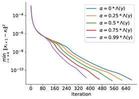
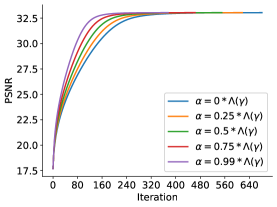
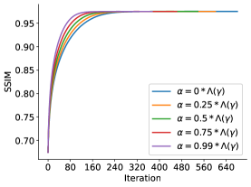
Figure 1: Effect of $\alpha$ in Algorithm 2 for solving DeTik model on ‘butterfly’ with Ker1 and noise level $2.55$. Increasing the extrapolation parameter $\alpha$ speeds-up the convergence of the algorithm. This increased convergence speed does not alter the quality of the proposed restoration.

In Fig. 1, we report the effect of $\alpha$ on ‘butterfly’ with Ker1 and noise level $2.55$. More specifically, the evolution curves of the convergence of residual $\left\|{\bf x}^{k+1}-{\bf x}^{k}\right\|$ at rate $\min_{j\leq k}\left\|{\bf x}^{j+1}-{\bf x}^{j}\right\|^{2}$, PSNR and SSIM values with respect to the number of iterations are presented, which showcases the advantage of the proposed extrapolation step. Furthermore, the detailed results include iteration number (Iter.), computational time in seconds (Time(s)), recovered PSNR (dB), and SSIM for three tested images (butterfly, leaves, and starfish) in Sect3C with different levels of noise are reported in Appendix A. From the presented results, we can see that Algorithm 2 exhibits improved performance as the extrapolation stepsize $\alpha$ increases, particularly in terms of computational cost. In our subsequent experiments, we set $\alpha=0.99*\Lambda(\gamma)$ for a given $\gamma$ to obtain results more efficiently.

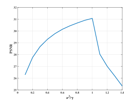
PSNR value along with $\gamma_{\nu}$

$\gamma_{\nu}=0.01$

$\gamma_{\nu}=1$

$\gamma_{\nu}=1.3$

Figure 2: Influence of the parameter $\gamma_{\nu}=\frac{\nu^{2}}{\gamma}$ for deblurring with DeTik model. First column: average PSNR along with the $\gamma_{\nu}$. The other parameters are fixed. Remaining columns: visual results for deblurring ‘leaves’ with various $\gamma_{\nu}$.

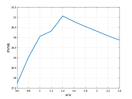
PSNR value along with $\sigma_{\nu}$

$\sigma_{\nu}=0.6$

$\sigma_{\nu}=1.4$

$\sigma_{\nu}=10$

Figure 3: Influence of the parameter $\sigma_{\nu}$ for deblurring with DeTik model. First column: average PSNR along with the $\sigma_{\nu}$. The other parameters are fixed. Remaining columns: visual results for deblurring ‘leaves’ with various $\sigma_{\nu}$.

5.2 Parameter analysis

In this subsection, we study the influence of the parameters and initialization of Algorithm 2 for solving the DeTik model. Recall that DeTik can be read as

$$\min_{{\bf x}\in\mathbb{R}^{n}}\frac{1}{2\nu^{2}}\|A{\bf x}-{\bf b}\|^{2}+\frac{1}{\gamma}\phi_{\sigma}({\bf x})+\frac{\beta}{2}\|{\bf x}\|^{2},$$

where $\nu$ and $\sigma$ are the noise levels of the synth input image and the denoiser $\phi_{\sigma}$, respectively. We fix model parameter $\beta$ for different noise levels as that in the last subsection, and roughly estimate $\sigma$ proportionally to the input noise level $\nu$ as $\sigma=\sigma_{\nu}*\nu$, where $\sigma_{\nu}$ is a positive constant. Consequently, the parameters we will be testing are $\gamma_{\nu}=\frac{\nu^{2}}{\gamma}$ and $\sigma_{\nu}=\sigma/\nu$.

In Fig. 2, we display the average PSNR value of Set3C using 10 tested blur kernels under a noise level of $2.55$, where $\gamma_{\nu}$ ranges from $0.1$ to $1.4$ with a step size of $0.1$. From the results, we can see that the instances with $\gamma_{\nu}$ values around 1 exhibit superior performance compared to other cases. This observation is further supported by the restored images on the right-hand side, which demonstrate that the quality of that corresponding to $\gamma_{\nu}=1$ is better than those for $\gamma_{\nu}=0.01$ and $\gamma_{\nu}=1.3$. When $\gamma_{\nu}=0.01$, the noise is removed, but the blur remains. for a larger value of $\gamma_{\nu}=1.3$, both the noise and blur remain. Hence, in our experiments, we chose $\gamma_{\nu}=1$ to address the noise level of $2.55$. Next, we test the effect of the parameter $\sigma_{\nu}$ and present the average PSNR value of Set3C with 10 tested blur kernels under noise level $2.55$ for $\sigma_{\nu}\in[0.6,2.4]$ with a step size $0.2$ in Fig. 3. The results indicate that almost no deblurring occurs when the value of $\sigma_{\nu}$ is small. Conversely, as $\sigma_{\nu}$ increases, excessive smoothing takes place, resulting in the loss of image details. Based on both the curve analysis and the visual outcomes, we select $\sigma_{\nu}\in[1,2]$.

We further investigate the impact of the initialization of Algorithm 2. In Fig. 4, we plot the average PSNR value of Set3C obtained from 10 tested blur kernels under a noise level of $2.55$. Due to the nonconvex regularizer, the proposed scheme is sensitive to initial value. Following the setting of [28], the initial ${\bf x}^{0}$ is varied with different noise levels: $\{0.01,2.55,5,7.5,10\}$. Based on the PSNR curve and visual quality in Fig. 4, we can see that a suitable initial input is crucial for the image deblurring task. When an initial input closely resembles the ground truth image, certain images may not undergo further iterations and terminate prematurely, particularly when the stopping criteria remain unchanged. On the other hand, if a heavily noisy image serves as the initial input, the iteration process progresses smoothly. However, the resulting image retains the heavy noise due to the low-level denoiser’s inability to effectively handle such noise levels. In our experiments, we adopt the observation as the initial input to ensure the validity of the obtained results.

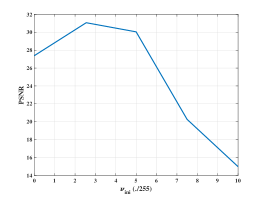
PSNR value along with $\nu_{init}$

$\nu_{init}=0.01/255$

$\nu_{init}=2.55/255$

$\nu_{init}=10/255$

Figure 4: Influence of the initialitation ${\bf x}^{0}$ for deblurring with DeTik model. First column: average PSNR along with different ${\bf x}^{0}$. The other parameters are fixed. Remaining columns: visual results for deblurring ‘leaves’ with various ${\bf x}^{0}$.

5.3 Image deblurring and super-resolution

In this subsection, we are devoted to demonstrating the effectiveness and robustness of the proposed Algorithm 2 and Algorithm 3 by solving image deblurring and super-resolution problems.

As discussed in Section 4.1, Algorithm 2 can be utilized to solve DeTik model due to the smoothness of $f_{1}({\bf x})=\frac{1}{2\nu^{2}}\|A{\bf x}-{\bf b}\|^{2}$, where $\nu$ is the noise level; Algorithm 3 can be used to solve DeBox model mentioned in Eq. 48. We first determine an appropriate $\gamma$ satisfying Section 3.1 and set $\alpha=0.99*\Lambda(\gamma)$. We consider Gaussian noise with 3 noise levels $\nu\in\{2.55,7.65,12.75\}/255$, i.e., $\nu\in\{0.01,0.03,0.05\}$, and 2 scale factors $\times 2,\times 3$. For the tested noise levels, we set $\sigma=\{1.4\nu,0.7\nu,0.6\nu\}$, $\nu^{2}/\gamma=\{1,0.9,0.6\}$ in Algorithm 2 for both image deblurring and super-resolution. For all noise levels, we set $\sigma=\{2\nu,1\nu,0.75\nu\}$ and $\nu^{2}/\gamma=\{5,1.5,1\}$ in Algorithm 3 for both tasks. We test the proposed algorithms for different tasks and compare the numerical results recovered by DeTik and BoxTik.

Table 1: Numerical results (PSNR(dB)) of our DeTik and BoxTik for image deblurring with Ker1 and 3 noise levels on Dataset Set3C.

Noise Level	2.55			7.65			12.75
Images	Butterfly	Leaves	Starfish	Butterfly	Leaves	Starfish	Butterfly	Leaves	Starfish
Degraded	17.68	16.50	21.56	17.48	16.34	21.09	17.10	16.06	20.28
DeTik	33.18	34.02	33.14	29.91	30.34	29.78	27.94	28.06	27.58
BoxTik	33.62	33.80	33.53	29.75	30.20	29.59	27.90	27.96	27.57

For the image deblurring task, we test four classical datasets, i.e., Set3C, Set14, Kodak24, and Set17, with different blur kernels and noise levels. For the sake of brevity, we present the image deblur results of Ker1 with various noise levels on Set3C in Table 1, and more results can be found in Appendix B. Our proposed methods demonstrate competitive performance in the task of image deblurring across different noise levels. On the other hand, the visual results of image ‘powerpoint2002’ in Set14 degraded by the blur Ker6 and noise level $12.75$ can be found in Fig. 5. To assess the convergence of the proposed algorithms in the experimental aspect, the evolution and energy curves are plotted and presented alongside the corresponding recovered images.

For the image super-resolution task, we set the scale factor as $\times 2$ and $\times 3$. Meanwhile, the blur and noise (mentioned in the deblurring task) are also considered in the experiments. The image super-resolution results on datasets Set5, CBSD68, and Urban100 are reported in Appendix B. More specifically, we report the numerical results on Set5 in Table 2. Furthermore, the visual results for noise level $7.65$ with blur Ker8 and scale factor $\times 2$ are shown in Fig. 6. The evolution and energy curves demonstrate the convergence of the proposed approaches in the experiment, which aligns with our theoretical results.

Table 2: Numerical results (PSNR(dB)) of our DeTik and BoxTik for image super-resolution with Ker1 and 3 noise levels and scales $\times 2$ and $\times 3$ on Dataset Set5.

Scales	Noise Level	2.55					7.65					12.75
	Images	Baby	Bird	Butterfly	Head	Woman	Baby	Bird	Butterfly	Head	Woman	Baby	Bird	Butterfly	Head	Woman
$\times 2$	Degraded	28.82	24.73	17.75	25.52	22.73	27.61	24.23	17.64	24.93	22.41	25.90	23.36	17.43	23.94	21.82
	DeTik	33.93	31.90	27.88	29.17	30.63	32.49	29.75	26.42	28.53	29.02	31.51	27.87	24.67	27.74	26.81
	BoxTik	34.26	31.85	27.19	29.19	30.51	32.45	29.53	26.16	28.32	28.89	31.42	27.85	24.77	27.63	26.95
$\times 3$	Degraded	28.75	24.72	17.75	25.43	22.66	27.20	24.05	17.61	24.65	22.23	25.15	22.94	17.34	23.40	21.47
	DeTik	32.40	29.17	22.51	28.29	27.44	31.51	27.59	23.68	27.77	26.47	30.46	26.05	22.35	27.20	25.14
	BoxTik	32.53	29.09	22.91	27.67	27.06	31.54	27.44	23.37	27.69	26.45	30.63	26.15	22.44	27.15	25.20

(a) Original

(b) Observed (18.14 dB)

(c) DeTik (30.04 dB)

(d) BoxTik (30.48 dB)

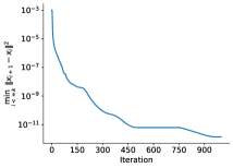
(e) Evolution of (c)

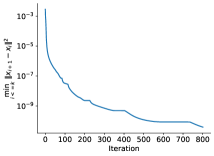
(f) Evolution of (d)

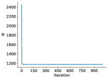
(g) $\Theta_{\alpha,\gamma}$ value of (c)

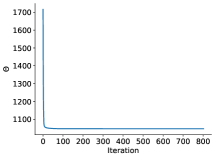
(h) $\Theta_{\alpha,\gamma}$ value of (d)

Figure 5: The deblurring results of DeTik and BoxTik on image degradation with Ker6 and noise level $12.75$. The evolution and $\Theta_{\alpha,\gamma}$ value along with the number of iterations.

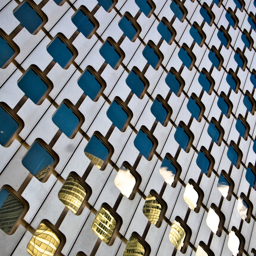
(a) Original

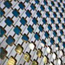
(b) Observed (18.03 dB)

(c) DeTik (24.82 dB)

(d) BoxTik (24.79 dB)

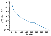
(e) Evolution of (c)

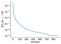
(f) Evolution of (d)

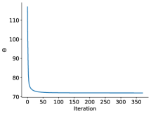
(g) $\Theta_{\alpha,\gamma}$ value of (c)

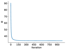
(h) $\Theta_{\alpha,\gamma}$ value of (d)

Figure 6: The super-resolution results of DeTik and BoxTik on image degradation with scale ($\times 2$) Ker8 and noise level $7.65$. The evolution and $\Theta_{\alpha,\gamma}$ value along with the number of iterations.

Table 3: Comparison on average image deblurring results (PSNR(dB)) of the state-of-the-art methods with our methods on Set3C, Set14, and Set17 datasets.

Datasets	Noise Level	Degraded	DWDN	DP-IRCNN	DPIR	DREDDUN	Alg. 1	Alg. 2	ADMM	Alg. 3
							TVTik	DeTik	TVBox	DeBox
Set3C	2.55	19.93	30.92	30.92	32.55	30.71	29.46	30.98	28.84	31.24
	7.65	19.52	28.62	27.60	28.60	28.62	25.10	28.78	25.18	28.62
	12.75	18.84	26.92	25.93	26.80	26.97	23.34	27.08	23.39	27.08
Set14	2.55	22.82	31.08	30.64	31.76	31.16	28.47	30.17	27.68	30.08
	7.65	22.10	28.41	28.13	28.79	28.57	26.68	28.47	26.06	28.33
	12.75	21.03	27.20	27.03	27.32	27.38	25.30	27.30	25.10	27.32
Set17	2.55	25.28	33.14	32.35	33.98	33.41	30.56	32.60	30.67	32.43
	7.65	24.07	30.39	29.83	30.64	30.62	27.73	30.64	27.85	30.55
	12.75	22.55	28.93	28.74	29.40	29.24	26.33	29.25	26.54	29.29

5.4 Comparison with state-of-the-art methods

In the preceding subsections, we have substantiated the validity of the proposed algorithm in handling both smooth and non-smooth objective functions. However, these evaluations alone do not entirely showcase the advantage of our method. Hence, in this subsection, we conduct a comparative analysis with state-of-the-art methods to provide further evidence of the exceptional effectiveness of our approach.

(a) Original

(b) Observed (23.02 dB)

(c) DWDN (31.05 dB)

(d) DP-IRCNN (31.22 dB)

(e) DPIR (31.97 dB)

(f) DREDDUN (31.19 dB)

(g) DeTik (32.05 dB)

(h) DeBox (31.61 dB)

Figure 7: Image deblurring results with Ker9 and noise level 12.75. (g) is the result of proposed Algorithm 2 for DeTik; (h) is the result of the proposed Algorithm 3 for DeBox.

5.4.1 Comparisons with advanced deblurring models

Following the implementation of the plug-and-play strategy, our proposed method integrates a denoiser into the objective function. Consequently, several methods that employ the same strategy are compared. While these methods yield competitive results, it is important to note that our proposed method holds a distinct advantage in terms of theoretical analysis. Specifically, our method guarantees convergence, whereas not all of the compared methods provide such a guarantee. In this paper, some plug-and-play methods and unrolling models DWDN [18], DPIR [78] with IRCNN [80] (DP-IRCNN), DPIR [78] with DRUNet (DPIR), and DREDDUN [30] are compared. All the compared codes were obtained either from the official published versions or were graciously provided by the authors themselves.

To provide more comprehensive results of the image deblurring, we compiled the average results for 10 blur kernels and 3 noise levels in Table 3. We list the results of the proposed two algorithms with two cases, respectively. From the numerical results, it becomes evident that our DeTik and DeBox yield competitive performance compared to deep learning-based plug-and-play and unrolling methods. Nevertheless, it is important to note that the traditional TVTik and TVBox cases may exhibit less satisfactory results, which is understandable considering that deep learning-based models have the advantage of leveraging more prior information compared to traditional priors. Furthermore, the visual results are depicted in Fig. 7 for a more comprehensive illustration. Note that we only present our PnP-based results (DeTik and DeBox) for visual comparison. We can see that although the PnP-based methods usually cause over-smoothing, the proposed algorithms (DeTik and DeBox) exhibit superior performance in detail restoration compared to the other methods.

Table 4: Comparison on average image super-resolution results (PSNR(dB)) of the state-of-the-art methods with our methods on Set5 and Urban100 datasets.

Scales	Datasets	Noise Level	Bicubic	USRNet	DP-IRCNN	DPIR	DREDDUN	Alg. 1	Alg. 2	ADMM	Alg. 3
								TVTik	DeTik	TVBox	DeBox
$\times 2$	Set5	2.55	24.21	30.75	29.33	31.07	30.49	28.16	30.29	27.70	30.51
		7.65	23.48	29.38	27.76	28.81	28.46	26.59	29.16	26.04	29.12
		12.75	22.45	27.98	26.96	27.60	27.34	23.26	27.91	24.40	27.99
	Urban100	2.55	19.15	25.67	25.34	25.40	25.43	21.23	24.10	21.51	23.86
		7.65	18.93	24.49	23.69	24.52	23.81	19.86	24.34	20.80	23.18
		12.75	18.53	22.92	22.68	23.18	22.89	19.24	23.29	19.81	22.34
$\times 3$	Set5	2.55	23.29	30.11	27.99	28.95	28.55	25.79	28.20	26.09	28.42
		7.65	22.71	28.19	26.52	27.22	27.11	25.19	27.65	25.72	27.64
		12.75	21.84	27.04	25.68	26.18	26.14	24.57	26.61	25.03	26.67
	Urban100	2.55	18.54	24.03	22.80	23.62	23.12	21.52	23.14	20.45	21.72
		7.65	18.35	22.12	21.90	22.36	21.67	20.05	21.65	19.92	21.45
		12.75	18.00	20.93	20.37	20.91	20.91	19.16	20.70	19.40	20.93

5.4.2 Comparisons with advanced super-resolution models

For image super-resolution task, USRNet [79], IRCNN [80] (DP-IRCNN), DPIR [78] with DRUNet (DPIR), and DREDDUN [30] are compared. All the compared codes used in our study were obtained either from the official published versions or were graciously provided by the authors themselves. Note that when addressing the image super-resolution task with sample scales $\times 2$ and $\times 3$, we simulated the degraded images by incorporating blur and noise during the sampling process. Specifically, we added 10 blur kernels and introduced the 3 Gaussian noises mentioned earlier.

The average image super-resolution results of the proposed algorithms with other advanced super-resolution models are listed in Table 4. We can see that our methods achieve competitive results under different scaling factors. While it is true that some compared methods outperform the proposed algorithm in some degradation cases, it is important to note that most of these methods lack convergence guarantees. Furthermore, we conducted a visual comparison of the renderings in Fig. 8, in which the proposed methods exhibit distinct advantages. Our proposed method excels in detail recovery when compared to other methods. Hence, based on both theoretical guarantees and experimental evidence, the algorithms we proposed exhibit distinct advantages when applied to image super-resolution tasks.

(a) Original

(b) Observed (18.56 dB)

(c) USRNet (22.28 dB)

(d) DP-IRCNN (22.10 dB)

(e) DPIR (22.51 dB)

(f) DREDDUN (21.53 dB)

(g) DeTik (22.84 dB)

(h) DeBox (22.62 dB)

Figure 8: Image super-resolution results with scale $\times 2$, Ker1 and noise level 7.65. (g) is the result of proposed Algorithm 2 for DeTik; (h) is the results of the proposed Algorithm 3 for DeBox.

6 Conclusions

This paper studied an extrapolated three-operator splitting method for solving a class of structural nonconvex optimization problems that minimize the sum of three functions. Our method extends the Davis-Yin splitting approach, which encompasses the widely-used forward-backward and Douglas-Rachford splitting methods, and introduces extrapolation techniques to handle nonconvex optimization problems. The convergence to a stationary point has been established by leveraging the Kurdyka-Łojasiewicz property. To further enhance the applicability, we applied the proposed splitting method within the Plug-and-Play (PnP) approach, incorporating a learned denoiser. The extrapolated PnP-based splitting methods replace the regularization step with a denoiser based on gradient step-based techniques, and we have provided theoretical guarantees for their convergence. This integration allows us to leverage the power of learning-based models. Furthermore, we have conducted extensive numerical experiments to evaluate the performance of our proposed methods on image deblurring and super-resolution problems. The results of these experiments have demonstrated the advantages and efficiency of the extrapolation strategy employed in our algorithmic framework. Importantly, our experiments have highlighted the superiority of the learning-based model with the PnP denoiser in terms of image quality.

In future research, we will consider the variants of the proposed method, such as incorporating line search, inexact solving techniques, and dynamically adapting parameter choices, to extend the applicability of our framework to a broader range of practical problems. Further theoretical investigations are warranted to establish convergence guarantees for splitting methods combined with other efficient PnP denoisers, such as the Bregman-based denoiser proposed in [26] for various Poisson inverse problems. In addition, investigating the potential applications of the proposed methods in the field of medical image processing is a crucial aspect of our future work.

Appendix A Experimental results on effect of extrapolation

We report the average image deblurring results under 10 different blur kernels and 3 noise levels in Table 5, which include iteration number (Iter.), computational time in seconds (Time(s)), recovered PSNR (dB), and SSIM for three tested images (butterfly, leaves, and starfish) in Sect3C with different levels of noise. From the presented results, we can see that Algorithm 2 exhibits improved performance as the extrapolation stepsize $\alpha$ increases, particularly in terms of computational cost. Increasing the extrapolation parameter $\alpha$ speeds-up the convergence of the algorithm. This increased convergence speed does not alter the quality of the proposed restoration.

Table 5: Parameter analysis of $\alpha$ in Algorithm 2 for image deblurring by DeTik model on the dataset Set3C with different noise levels.

$\alpha$	Image	butterfly				leaves				starfish
	Noise Level	2.55	7.65	12.75		2.55	7.65	12.75		2.55	7.65	12.75
0	Iter.	681	1001	512		436	596	428		388	396	513
	Time(s)	25.97	36.79	18.87		15.54	20.92	15.61		13.56	13.75	18.30
	PSNR	33.18	29.91	27.94		33.97	30.33	28.05		33.11	29.78	27.57
	SSIM	0.9760	0.9569	0.9367		0.9890	0.9760	0.9617		0.9551	0.9233	0.8866
$0.25*\Lambda(\gamma)$	Iter.	617	972	457		383	532	381		340	351	417
	Time(s)	22.54	37.87	17.03		13.13	19.00	13.72		11.42	12.40	14.74
	PSNR	33.18	29.91	27.94		33.97	30.33	28.05		33.11	29.78	27.57
	SSIM	0.9760	0.9569	0.9367		0.9890	0.9760	0.9617		0.9551	0.9233	0.8866
$0.50*\Lambda(\gamma)$	Iter.	550	901	403		332	467	226		297	308	396
	Time(s)	20.07	36.18	15.07		11.79	16.32	12.07		10.11	10.51	13.88
	PSNR	33.18	29.91	27.94		33.97	30.33	28.05		33.11	29.78	27.57
	SSIM	0.9760	0.9569	0.9367		0.9890	0.9760	0.9617		0.9551	0.9233	0.8866
$0.75*\Lambda(\gamma)$	Iter.	463	873	348		279	405	317		251	265	507
	Time(s)	16.77	37.86	12.46		10.06	14.28	10.99		8.71	9.35	17.20
	PSNR	33.18	29.91	27.94		33.9	30.33	28.05		33.11	29.78	27.58
	SSIM	0.9760	0.9569	0.9367		0.9890	0.9760	0.9617		0.9551	0.9233	0.8866
$0.99*\Lambda(\gamma)$	Iter.	375	861	491		225	344	26		204	223	276
	Time(s)	13.63	32.35	18.41		7.66	12.10	9.21		6.69	7.69	9.31
	PSNR	33.18	29.91	27.95		33.97	30.33	28.05		33.14	29.78	27.57
	SSIM	0.9760	0.9569	0.9367		0.9890	0.9760	0.9617		0.9551	0.9233	0.8866

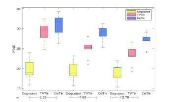
Set3C

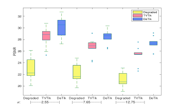
Set14

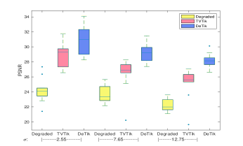
Kodak24

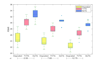
Set17

Figure 9: Average results (PSNR(dB)) of TVTik and DeTik for image deblurring with 10 different blur kernels and 3 noise levels on Set3C, Set14, Kodak24, and Set17 datasets.

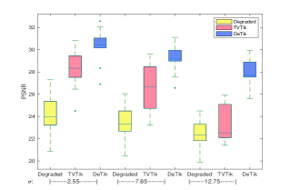
Set5 ($\times 2$)

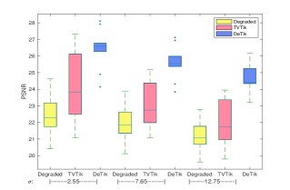
CBSD68 ($\times 2$)

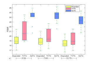
Urban100 ($\times 2$)

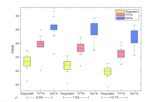
Set5 ($\times 3$)

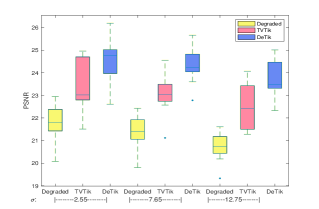
CBSD68 ($\times 3$)

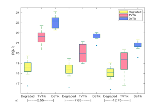
Urban100 ($\times 3$)

Figure 10: Average results (PSNR(dB)) of TVTik and DeTik for image super-resolution with 2 scales ($\times 2$ and $\times 3$), 10 different blur kernels and 3 noise levels on Set5, CBSD68, and Urban100 datasets.

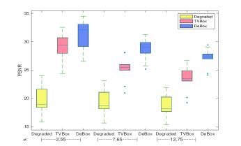
Set3C

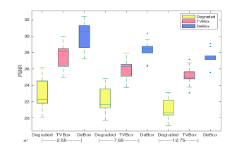
Set14

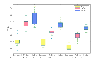
Kodak24

Set17

Figure 11: Average results (PSNR(dB)) of TVBox and DeBox for image deblurring with 10 different blur kernels and 3 noise levels on Set3C, Set14, Kodak24, and Set17 datasets.

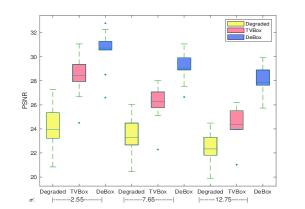
Set5 ($\times 2$)

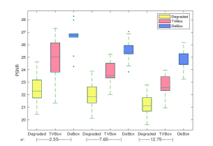
CBSD68 ($\times 2$)

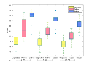
Urban100 ($\times 2$)

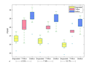
Set5 ($\times 3$)

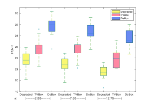
CBSD68 ($\times 3$)

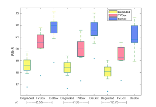
Urban100 ($\times 3$)

Figure 12: Average numerical results (PSNR(dB)) of TVBox and DeBox for image super-resolution with 2 scales ($\times 2$ and $\times 3$), 10 different blur kernels and 3 noise levels on Set5, CBSD68, and Urban100 datasets.

Appendix B Experimental results on robustness of Algorithm 2 and Algorithm 3

To further demonstrate the effectiveness of the proposed methods, we compare the results recovered by the model TVTik and DeTik in Fig. 9 and Fig. 10, and the model BoxTik and TVBox in Fig. 11 and Fig. 12, for image deblurring and super-resolution, respectively.

We use the Matlab built-in function ‘boxplot’ to create a box plot. As shown in Fig. 9, each picture contains 9 boxes. The yellow, pink, and blue boxes represent the average PSNR values of the degraded images, the images restored by TVTik and DeTik, and the first, second, and third sets of yellow, pink, and blue boxes correspond to the noise levels of $2.55$, $7.65$, and $12.75$, respectively. On each box, the central mark indicates the median, and the bottom and top edges of the box indicate the $25$th and $75$th percentiles. The whiskers extend to the most extreme data points not considered outliers, and the outliers are plotted individually using the dot symbol. From the box plot, we can see that the median of DeTik is higher than that of TVTik. Note that the TVTik model also enhances the quality of the degraded image when compared to the yellow boxes. These results demonstrate that Algorithm 2 is efficient in image restoration, as it successfully restores images affected by 10 different kernels and 3 different noise levels. Similarly to the deblurring results, the box plot is presented to show the super-resolution outcomes. The first and second rows of the box plot display the results of super-resolution under degradation with scale factors $\times 2$ and $\times 3$, respectively. The results presented in Fig. 10 also demonstrate that the proposed algorithm effectively solves the tested models, and DeTik outperforms TVTik in terms of recovery quality for image super-resolution.

For different noise levels and blur kernels, the average image restoration results of Set3C, Set14, Kodak24, and Set17 with box plot are demonstrated in Fig. 11. The yellow, pink, and blue boxes denote the average PSNR of the degraded images, the image restored by TVBox and DeBox. The first, second, and third sets of yellow, pink, and blue boxes correspond to the noise levels of $2.55$, $7.65$, and $12.75$, respectively. Similarly, the super-resolution results for two scale factors, $\times 2$ and $\times 3$, are presented in Fig. 12. The result demonstrates that the proposed method exhibits consistent and stable image restoration performance. From Fig. 11 and Fig. 12, we can see that Algorithm 3 effectively solves the DeBox model, and DeBox outperforms TVBox in terms of recovery quality for both image deblurring and super-resolution tasks. The experiment results also demonstrate that Algorithm 3 can handle the minimization with the non-differentiable term.

References

• [1] M. Ahookhosh, A. Themelis, and P. Patrinos, A Bregman forward-backward linesearch algorithm for nonconvex composite optimization: superlinear convergence to nonisolated local minima, SIAM Journal on Optimization, 31 (2021), pp. 653–685.
• [2] H. Attouch, J. Bolte, P. Redont, and A. Soubeyran, Proximal alternating minimization and projection methods for nonconvex problems: An approach based on the Kurdyka-Łojasiewicz inequality, Mathematics of Operations Research, 35 (2010), pp. 438–457.
• [3] H. Attouch, J. Bolte, and B. F. Svaiter, Convergence of descent methods for semi-algebraic and tame problems: proximal algorithms, forward–backward splitting, and regularized Gauss–Seidel methods, Mathematical Programming, 137 (2013), pp. 91–129.
• [4] H. Attouch, J. Peypouquet, and P. Redont, A dynamical approach to an inertial forward-backward algorithm for convex minimization, SIAM Journal on Optimization, 24 (2014), pp. 232–256.
• [5] A. Barakat and P. Bianchi, Convergence rates of a momentum algorithm with bounded adaptive step size for nonconvex optimization, in Asian Conference on Machine Learning, PMLR, 2020, pp. 225–240.
• [6] A. Beck and M. Teboulle, A fast iterative shrinkage-thresholding algorithm for linear inverse problems, SIAM Journal on Imaging Sciences, 2 (2009), pp. 183–202.
• [7] F. Bian and X. Zhang, A three-operator splitting algorithm for nonconvex sparsity regularization, SIAM Journal on Scientific Computing, 43 (2021), pp. 2809–2839.
• [8] J. Bolte, S. Sabach, and M. Teboulle, Proximal alternating linearized minimization for nonconvex and nonsmooth problems, Mathematical Programming, 146 (2014), pp. 459–494.
• [9] R. I. Boţ, E. R. Csetnek, and S. C. László, An inertial forward–backward algorithm for the minimization of the sum of two nonconvex functions, EURO Journal on Computational Optimization, 4 (2016), pp. 3–25.
• [10] G. T. Buzzard, S. H. Chan, S. Sreehari, and C. A. Bouman, Plug-and-play unplugged: Optimization-free reconstruction using consensus equilibrium, SIAM Journal on Imaging Sciences, 11 (2018), pp. 2001–2020.
• [11] C. Castera, J. Bolte, C. Févotte, and E. Pauwels, An inertial newton algorithm for deep learning, The Journal of Machine Learning Research, 22 (2021), pp. 5977–6007.
• [12] C. Chen, S. Ma, and J. Yang, A general inertial proximal point algorithm for mixed variational inequality problem, SIAM Journal on Optimization, 25 (2015), pp. 2120–2142.
• [13] R. Cohen, Y. Blau, D. Freedman, and E. Rivlin, It has potential: Gradient-driven denoisers for convergent solutions to inverse problems, Advances in Neural Information Processing Systems, 34 (2021), pp. 18152–18164.
• [14] P. L. Combettes and J.-C. Pesquet, Fixed point strategies in data science, IEEE Transactions on Signal Processing, 69 (2021), pp. 3878–3905.
• [15] L. Condat, D. Kitahara, A. Contreras, and A. Hirabayashi, Proximal splitting algorithms for convex optimization: A tour of recent advances, with new twists, SIAM Review, 65 (2023), pp. 375–435.
• [16] D. Davis and W. Yin, A three-operator splitting scheme and its optimization applications, Set-Valued and Variational Analysis, 25 (2017), pp. 829–858.
• [17] L.-J. Deng, R. Glowinski, and X.-C. Tai, A new operator splitting method for the Euler elastica model for image smoothing, SIAM Journal on Imaging Sciences, 12 (2019), pp. 1190–1230.
• [18] J. Dong, S. Roth, and B. Schiele, Deep wiener deconvolution: Wiener meets deep learning for image deblurring, Advances in Neural Information Processing Systems, 33 (2020), pp. 1048–1059.
• [19] R. G. Gavaskar, C. D. Athalye, and K. N. Chaudhury, On plug-and-play regularization using linear denoisers, IEEE Transactions on Image Processing, 30 (2021), pp. 4802–4813.
• [20] T. Goldstein and S. Osher, The split bregman method for l1-regularized problems, SIAM Journal on Imaging Sciences, 2 (2009), pp. 323–343.
• [21] K. Guo and D. Han, A note on the Douglas–Rachford splitting method for optimization problems involving hypoconvex functions, Journal of Global Optimization, 72 (2018), pp. 431–441.
• [22] K. Guo, D. Han, and X. Yuan, Convergence analysis of Douglas–Rachford splitting method for “strongly+ weakly” convex programming, SIAM Journal on Numerical Analysis, 55 (2017), pp. 1549–1577.
• [23] D. Han, A survey on some recent developments of alternating direction method of multipliers, Journal of the Operations Research Society of China, (2022), pp. 1–52.
• [24] J. Hertrich, S. Neumayer, and G. Steidl, Convolutional proximal neural networks and plug-and-play algorithms, Linear Algebra and its Applications, 631 (2021), pp. 203–234.
• [25] S. Hurault, A. Chambolle, A. Leclaire, and N. Papadakis, Convergent Plug-and-Play with proximal denoiser and unconstrained regularization parameter, arXiv preprint arXiv:2311.01216, (2023).
• [26] S. Hurault, U. Kamilov, A. Leclaire, and N. Papadakis, Convergent Bregman plug-and-play image restoration for Poisson inverse problems, arXiv preprint arXiv:2306.03466, (2023).
• [27] S. Hurault, A. Leclaire, and N. Papadakis, Gradient step denoiser for convergent plug-and-play, in International Conference on Learning Representations (ICLR’22), 2022.
• [28] S. Hurault, A. Leclaire, and N. Papadakis, Proximal denoiser for convergent plug-and-play optimization with nonconvex regularization, in International Conference on Machine Learning, PMLR, 2022, pp. 9483–9505.
• [29] P. Jain, P. Kar, et al., Non-convex optimization for machine learning, Foundations and Trends® in Machine Learning, 10 (2017), pp. 142–363.
• [30] S. Kong, W. Wang, X. Feng, and X. Jia, Deep red unfolding network for image restoration, IEEE Transactions on Image Processing, 31 (2022), pp. 852–867.
• [31] S. G. Krantz and H. R. Parks, A primer of real analytic functions, Springer Science & Business Media, 2002.
• [32] P. Latafat and P. Patrinos, Asymmetric forward–backward–adjoint splitting for solving monotone inclusions involving three operators, Computational Optimization and Applications, 68 (2017), pp. 57–93.
• [33] H. Le, N. Gillis, and P. Patrinos, Inertial block proximal methods for non-convex non-smooth optimization, in International Conference on Machine Learning, PMLR, 2020, pp. 5671–5681.
• [34] G. Li and T. K. Pong, Douglas–Rachford splitting for nonconvex optimization with application to nonconvex feasibility problems, Mathematical Programming, 159 (2016), pp. 371–401.
• [35] J. Li, C. Huang, R. Chan, H. Feng, M. K. Ng, and T. Zeng, Spherical image inpainting with frame transformation and data-driven prior deep networks, SIAM Journal on Imaging Sciences, 16 (2023), pp. 1179–1196.
• [36] M. Li and Z. Wu, Convergence analysis of the generalized splitting methods for a class of nonconvex optimization problems, Journal of Optimization Theory and Applications, 183 (2019), pp. 535–565.
• [37] J. Liang, J. Fadili, and G. Peyré, A multi-step inertial forward-backward splitting method for non-convex optimization, Advances in Neural Information Processing Systems, 29 (2016).
• [38] J. Liang, J. Fadili, and G. Peyré, Activity identification and local linear convergence of forward–backward-type methods, SIAM Journal on Optimization, 27 (2017), pp. 408–437.
• [39] S. B. Lindstrom and B. Sims, Survey: sixty years of Douglas–Rachford, Journal of the Australian Mathematical Society, 110 (2021), pp. 333–370.
• [40] H. Liu, X.-C. Tai, and R. Glowinski, An operator-splitting method for the gaussian curvature regularization model with applications to surface smoothing and imaging, SIAM Journal on Scientific Computing, 44 (2022), pp. A935–A963.
• [41] J. Liu, S. Asif, B. Wohlberg, and U. Kamilov, Recovery analysis for plug-and-play priors using the restricted eigenvalue condition, Advances in Neural Information Processing Systems, 34 (2021), pp. 5921–5933.
• [42] Y. Liu and W. Yin, An envelope for Davis-Yin splitting and strict saddle-point avoidance, Journal of Optimization Theory and Applications, 181 (2019), pp. 567–587.
• [43] D. A. Lorenz and T. Pock, An inertial forward-backward algorithm for monotone inclusions, Journal of Mathematical Imaging and Vision, 51 (2015), pp. 311–325.
• [44] Y. Nesterov, Introductory lectures on convex optimization: A basic course, vol. 87, Springer Science & Business Media, 2003.
• [45] P. Ochs, Y. Chen, T. Brox, and T. Pock, ipiano: Inertial proximal algorithm for nonconvex optimization, SIAM Journal on Imaging Sciences, 7 (2014), pp. 1388–1419.
• [46] S. Ono, Primal-dual plug-and-play image restoration, IEEE Signal Processing Letters, 24 (2017), pp. 1108–1112.
• [47] J.-C. Pesquet, A. Repetti, M. Terris, and Y. Wiaux, Learning maximally monotone operators for image recovery, SIAM Journal on Imaging Sciences, 14 (2021), pp. 1206–1237.
• [48] D. N. Phan and N. Gillis, An inertial block majorization minimization framework for nonsmooth nonconvex optimization, Journal of Machine Learning Research, 24 (2023), pp. 1–41.
• [49] T. Pock and S. Sabach, Inertial proximal alternating linearized minimization (iPALM) for nonconvex and nonsmooth problems, SIAM Journal on Imaging Sciences, 9 (2016), pp. 1756–1787.
• [50] B. T. Polyak, Some methods of speeding up the convergence of iteration methods, Ussr Computational Mathematics and Mathematical Physics, 4 (1964), pp. 1–17.
• [51] H. Raguet, J. Fadili, and G. Peyré, A generalized forward-backward splitting, SIAM Journal on Imaging Sciences, 6 (2013), pp. 1199–1226.
• [52] E. T. Reehorst and P. Schniter, Regularization by denoising: Clarifications and new interpretations, IEEE Transactions on Computational Imaging, 5 (2018), pp. 52–67.
• [53] R. T. Rockafellar and R. J.-B. Wets, Variational analysis, vol. 317, Springer Science & Business Media, 2009.
• [54] L. I. Rudin, S. Osher, and E. Fatemi, Nonlinear total variation based noise removal algorithms, Physica D: Nonlinear Phenomena, 60 (1992), pp. 259–268.
• [55] E. Ryu, J. Liu, S. Wang, X. Chen, Z. Wang, and W. Yin, Plug-and-play methods provably converge with properly trained denoisers, International Conference on Machine Learning, (2019), pp. 5546–5557.
• [56] E. K. Ryu, A. B. Taylor, C. Bergeling, and P. Giselsson, Operator splitting performance estimation: Tight contraction factors and optimal parameter selection, SIAM Journal on Optimization, 30 (2020), pp. 2251–2271.
• [57] A. Salim, L. Condat, K. Mishchenko, and P. Richtárik, Dualize, split, randomize: Toward fast nonsmooth optimization algorithms, Journal of Optimization Theory and Applications, 195 (2022), pp. 102–130.
• [58] S. Setzer, Operator splittings, bregman methods and frame shrinkage in image processing, International Journal of Computer Vision, 92 (2011), pp. 265–280.
• [59] S. Sreehari, S. V. Venkatakrishnan, B. Wohlberg, G. T. Buzzard, L. F. Drummy, J. P. Simmons, and C. A. Bouman, Plug-and-play priors for bright field electron tomography and sparse interpolation, IEEE Transactions on Computational Imaging, 2 (2016), pp. 408–423.
• [60] Y. Sun, B. Wohlberg, and U. S. Kamilov, An online plug-and-play algorithm for regularized image reconstruction, IEEE Transactions on Computational Imaging, 5 (2019), pp. 395–408.
• [61] Y. Sun, Z. Wu, X. Xu, B. Wohlberg, and U. S. Kamilov, Scalable plug-and-play ADMM with convergence guarantees, IEEE Transactions on Computational Imaging, 7 (2021), pp. 849–863.
• [62] Y. Tang, M. Wen, and T. Zeng, Preconditioned three-operator splitting algorithm with applications to image restoration, Journal of Scientific Computing, 92 (2022), pp. 1–26.
• [63] A. Themelis and P. Patrinos, Douglas–Rachford splitting and ADMM for nonconvex optimization: Tight convergence results, SIAM Journal on Optimization, 30 (2020), pp. 149–181.
• [64] A. Themelis, L. Stella, and P. Patrinos, Forward-backward envelope for the sum of two nonconvex functions: Further properties and nonmonotone linesearch algorithms, SIAM Journal on Optimization, 28 (2018), pp. 2274–2303.
• [65] A. Themelis, L. Stella, and P. Patrinos, Douglas–Rachford splitting and ADMM for nonconvex optimization: accelerated and newton-type linesearch algorithms, Computational Optimization and Applications, 82 (2022), pp. 395–440.
• [66] T. Tirer and R. Giryes, Image restoration by iterative denoising and backward projections, IEEE Transactions on Image Processing, 28 (2018), pp. 1220–1234.
• [67] S. V. Venkatakrishnan, C. A. Bouman, and B. Wohlberg, Plug-and-play priors for model based reconstruction, in 2013 IEEE Global Conference on Signal and Information Processing, IEEE, 2013, pp. 945–948.
• [68] S. Villa, S. Salzo, L. Baldassarre, and A. Verri, Accelerated and inexact forward-backward algorithms, SIAM Journal on Optimization, 23 (2013), pp. 1607–1633.
• [69] Q. Wang and D. Han, A generalized inertial proximal alternating linearized minimization method for nonconvex nonsmooth problems, Applied Numerical Mathematics, 189 (2023), pp. 66–87.
• [70] K. Wei, A. Aviles-Rivero, J. Liang, Y. Fu, H. Huang, and C.-B. Schönlieb, Tfpnp: Tuning-free plug-and-play proximal algorithms with applications to inverse imaging problems, The Journal of Machine Learning Research, 23 (2022), pp. 699–746.
• [71] T. Wu, W. Wu, Y. Yang, F.-L. Fan, and T. Zeng, Retinex image enhancement based on sequential decomposition with a plug-and-play framework, IEEE Transactions on Neural Networks and Learning Systems, (2023), pp. 1–14.
• [72] Z. Wu, C. Li, M. Li, and A. Lim, Inertial proximal gradient methods with Bregman regularization for a class of nonconvex optimization problems, Journal of Global Optimization, 79 (2021), pp. 617–644.
• [73] Z. Wu and M. Li, General inertial proximal gradient method for a class of nonconvex nonsmooth optimization problems, Computational Optimization and Applications, 73 (2019), pp. 129–158.
• [74] J. Yang and Y. Zhang, Alternating direction algorithms for ${L}_{1}$-problems in compressive sensing, SIAM Journal on Scientific Computing, 33 (2011), pp. 250–278.
• [75] P. Yin, Y. Lou, Q. He, and J. Xin, Minimization of ${L}_{1}$-${L}_{2}$ for compressed sensing, SIAM Journal on Scientific Computing, 37 (2015), pp. 536–583.
• [76] A. Yurtsever, V. Mangalick, and S. Sra, Three operator splitting with a nonconvex loss function, in International Conference on Machine Learning, PMLR, 2021, pp. 12267–12277.
• [77] J. Zeng, T. T.-K. Lau, S. Lin, and Y. Yao, Global convergence of block coordinate descent in deep learning, in International Conference on Machine Learning, PMLR, 2019, pp. 7313–7323.
• [78] K. Zhang, Y. Li, W. Zuo, L. Zhang, L. Van Gool, and R. Timofte, Plug-and-play image restoration with deep denoiser prior, IEEE Transactions on Pattern Analysis and Machine Intelligence, 44 (2021), pp. 6360–6376.
• [79] K. Zhang, L. Van Gool, and R. Timofte, Deep unfolding network for image super-resolution, in IEEE Conference on Computer Vision and Pattern Recognition, 2020, pp. 3217–3226.
• [80] K. Zhang, W. Zuo, S. Gu, and L. Zhang, Learning deep cnn denoiser prior for image restoration, in IEEE Conference on Computer Vision and Pattern Recognition, 2017, pp. 3929–3938.