OpenGraph: Towards Open Graph Foundation Models

Abstract.

Graph learning has become indispensable for interpreting and harnessing relational data in diverse fields, ranging from recommendation systems to social network analysis. In this context, a variety of graph neural networks (GNNs) have emerged as promising methodologies for encoding the structural information of graphs. By effectively capturing the graph’s underlying structure, these GNNs have shown great potential in enhancing performance in graph learning tasks, such as link prediction and node classification. However, despite their successes, a significant challenge persists: these advanced methods often face difficulties in generalizing to unseen graph data that significantly differs from the training instances. In this work, our aim is to advance the graph learning paradigm by developing a general graph foundation model. This model is designed to understand the complex topological patterns present in diverse graph data, enabling it to excel in zero-shot graph learning tasks across different downstream datasets. To achieve this goal, we address several key technical challenges in our OpenGraph model. Firstly, we propose a unified graph tokenizer to adapt our graph model to generalize well on unseen graph data, even when the underlying graph properties differ significantly from those encountered during training. Secondly, we develop a scalable graph transformer as the foundational encoder, which effectively captures node-wise dependencies within the global topological context. Thirdly, we introduce a data augmentation mechanism enhanced by a large language model (LLM) to alleviate the limitations of data scarcity in real-world scenarios. Extensive experiments validate the effectiveness of our framework. By adapting our OpenGraph to new graph characteristics and comprehending the nuances of diverse graphs, our approach achieves remarkable zero-shot graph learning performance across various settings and domains.

1. Introduction

Graph learning has established itself as a core and indispensable methodology for unlocking the inherent power of relational data across a wide spectrum of fields. Its versatility and applicability span diverse domains, including recommender systems (he2020lightgcn, ), social network analysis (sankar2021graph, ), citation networks (lv2021we, ), and transportation networks (wang2020traffic, ). To effectively capture the intricate structures inherent in graphs, the adoption of Graph Neural Networks (GNNs) has become pervasive in learning representations for graph-structured data. GNNs are built on the foundation of recursive message passing, leveraging the inter-dependencies of nodes to incorporate high-order connectivities into the learned graph representations (ying2018graph, ; jin2020graph, ).

One of the primary challenges faced by current end-to-end graph neural networks is their heavy reliance on labeled data. This strong dependence on labeled data presents a primary obstacle in real-world situations, where obtaining a sufficient amount of accurately labeled data can be both expensive and challenging (liu2022graph, ; jin2021automated, ). Consequently, the labeled data that is available often exhibits problems of being sparse and of low quality. To tackle this issue, self-supervised learning (SSL) has emerged as a potential solution to enhance graph neural networks by leveraging augmented self-supervision signals. These methods typically adopt a learning pipeline that involves "pre-training" and "fine-tuning" with self-supervised pre-training tasks. In the context of self-supervised learning and pre-training on graphs, contrasive SSL has been the dominant approaches. For example, contrastive objectives are incorporated as self-supervised alignment loss to supplement the classical supervised task, Notable examples include DGI (velivckovic2018deep, ) and GraphCL (you2020graph, ). Further research, such as JOAO (you2021graph, ) and GCA (zhu2021graph, ), aims to automate the contrastive learning process through adaptive augmentation.

While graph pre-training techniques have demonstrated effectiveness in capturing intrinsic graph properties, they still encounter difficulties in achieving strong generalization from the pre-training phase to the downstream task-specific context (sun2023all, ), especially when confronted with distribution shifts in graph characteristics across diverse downstream domains (wu2021handling, ; gui2022good, ). For example, in recommender systems, there is a need to handle previously unseen user interaction graphs that arise from newly generated items, such as news articles or videos, in cold-start recommendation scenarios (chen2022generative, ). Furthermore, there is a desire to transfer the acquired knowledge from pre-trained graph domains to other downstream domains (zhang2022few, ). However, when these models are applied to unseen graphs, their performance significantly deteriorates. This decline can be attributed to the variations in graph characteristics observed in different downstream scenarios, including changes in node sets and feature semantics.

Recent research has explored the use of prompt-tuning as a task-specific alternative to fine-tuning, aiming to bridge the gap between pre-training and downstream objectives (sun2022gppt, ; liu2023graphprompt, ; fang2022universal, ). By merging the pre-training and prompt-tuning frameworks, these approaches enable a more efficient alignment of the pre-trained model’s understanding with the specific requirements of the downstream task. However, it is important to note that most of these frameworks assume that the training and testing graph data share the same node set and feature semantics. In practical scenarios, variations in node sets and feature semantics are common across diverse downstream graph domains. Therefore, further exploration is needed to enhance the generalization power of graph models and ensure their adaptability to various real-world downstream graphs.

Considering the aforementioned motivations and challenges, the objective of this work is to push the boundaries of graph learning by developing a versatile and scalable graph model. The primary aim is to equip the model with the capability of zero-shot learning, enabling it to effectively learn from and make accurate predictions on previously unseen graphs. However, building such a graph model is not a trival task and requires addressing several key challenges.

• C1: Node Token Set Shift across Different Graphs. One notable challenge in zero-shot graph learning is the shift in node token sets across different graphs. This discrepancy necessitates the model to proficiently reconcile the variations in node characteristics. It is crucial to generate universal graph tokens that possess the adaptability to effectively represent and comprehend arbitrary unseen graphs with diverse graph topological contexts.
  

• C2: Efficient Node-wise Dependency Modeling. In the realm of graph learning, nodes in large-scale graphs exhibit intricate dependencies on each other. It is crucial to comprehend both local and global inter-dependencies among all nodes for accurate prediction and effective learning. Yet, when it comes to modeling universal dependencies over extensive graphs, the efficiency of node-wise dependency encoding becomes vital in enhancing the performance and scalability of graph models.
  

• C3: Domain-Specific Data Scarcity. Data scarcity is a widespread challenge across various downstream domain tasks, and it arises from multiple factors. Privacy concerns, for example, restrict the collection of domain-specific user behavior graphs, resulting in limited data availability. Consequently, it becomes crucial to develop label-less learning frameworks within graph foundation models to effectively understand the relevant context of downstream tasks under conditions of data scarcity.

Present Work. To overcome these challenges, we present OpenGraph, a flexible graph model that excels in zero-shot graph learning, allowing it to capture the universal and transferable structural patterns across multiple domains or datasets. To address the first challenge C1, we introduce a graph tokenizer that efficiently transforms input graphs into unified token sequences. This is achieved by incorporating a topology-aware projection scheme, enabling the generation of universal graph tokens from arbitrary graphs, regardless of variations in node token sets. To conquer the second challenge, C2, we have developed a highly scalable graph transformer equipped with efficient self-attention using anchor sampling. This innovative approach ensures computational efficiency through a two-stage self-attention process. Additionally, we employ token sequence sampling to optimize the training process, leveraging sampled token sequences from the current batch. This reduces the sequence length while preserving the crucial graph context.

To tackle the challgne of C3, we introduce a novel approach that combines the power of large language models (LLMs) with data augmentation techniques for synthetic graph generation. Our goal is to enhance the pre-training process of our OpenGraph model by incorporating more downstream task-relevant context and gaining a deeper understanding of real-world graph characteristics. This is achieved through the generation of augmented graphs that closely resemble real-world instances. To achieve this, we employ an integration of the tree-of-prompt regularized with Gibbs sampling.

We conducted extensive experiments on a diverse range of publicly available graph datasets, encompassing various scales and types. The outcomes were truly remarkable, as our OpenGraph consistently showcased exceptional generalization capabilities across a wide array of settings. Particularly exciting is the fact that the zero-shot learning ability of OpenGraph surpassed baselines even in few-shot learning scenarios. This outcome lays the foundation for the development of graph foundation models, which have the potential to generalize effectively across diverse graph domains.

2. Preliminaries

Graph Representation Learning. A graph $\mathcal{G}$ consists of a set of nodes $\mathcal{V}$ and a set of edges $\mathcal{E}$. The edges $e=(v_{s},v_{t})\in\mathcal{E}$ represent observed relations between a source node $v_{s}$ and a target node $v_{t}$. Additionally, we define a feature matrix $\textbf{F}\in\mathbb{R}^{|\mathcal{V}|\times f}$ to capture the $f$-dimensional feature attributes of all nodes. Graph representation learning aims to capture meaningful node representations by transforming both the structural and attribute information into low-dimensional vector embeddings. These embeddings encode the patterns of inter-node dependencies and relationships, facilitating graph learning tasks such as link prediction and node classification.

The link prediction focuses on predicting the probability of establishing connections between node pairs $(v_{s},v_{t})$ that are not observed in the given data. The node classification task aims to assign a category to each node based on its features and relationships with other nodes. These tasks can be formally expressed:

$$\mathop{\arg\min}_{\mathbf{\Theta}_{f}}\mathcal{L}_{\text{node}}=-\sum_{v_{s},y_{s}}\Big{(}{f(v_{s},y_{s})}\leavevmode\nobreak\ /{\sum_{y^{\prime}_{s}\neq y_{s}}f(v_{s},y^{\prime}_{s})}\Big{)},$$

(1) $$\mathop{\arg\min}_{\mathbf{\Theta}_{f}}\mathcal{L}_{\text{link}}=-\sum_{v_{s},v_{t}}e_{s,t}f(v_{s},v_{t})-(1-e_{s,t})f(v_{s},v_{t})$$

Here, The link labels $e_{s,t}\in\{0,1\}$ indicate if node $v_{s}$ is connected to node $v_{t}$. $f$ denotes the prediction model with a learnable parameter set $\mathbf{\Theta}_{f}$. The node labels $y_{s}\in\mathcal{C}$ indicate the groundtruth category for node $v_{s}$, while $\mathcal{C}$ denotes the set of candidate categories.

Zero-shot Graph Learning. Although current graph learning methods demonstrate promising results in standard graph learning tasks, they face limitations when it comes to effectively generalizing across diverse domains. When these models are applied to new and unseen graphs, their performance noticeably decreases. This decline can be attributed to the variations in graph characteristics that exist across different downstream scenarios, such as changes in the node set and feature semantics. Existing models heavily depend on parameters that are specifically tailored to these graph-specific tokens, which include feature transformations and node embeddings. As a result, these models encounter challenges in their ability to effectively generalize and adapt to new graphs that possess distinct graph tokens and relational semantics.

Recognizing the limitations of current approaches, our research focuses on zero-shot graph learning. This task involves training a model on a set of graphs and evaluating its performance on different test graphs that do not share any graph tokens. The goal is to assess the ability of graph models to learn generalized graph topological structures and node-wise dependencies. To provide a formal definition of the zero-shot graph learning task:

$$\mathop{\arg\min}\nolimits_{f}\epsilon(\{\mathcal{G}_{t}\},f),\leavevmode\nobreak\ \leavevmode\nobreak\ \text{where}\leavevmode\nobreak\ \mathbf{\Theta}_{f}=\mathop{\arg\min}\nolimits_{\mathbf{\Theta}_{f}}\mathcal{L}(\{\mathcal{G}_{s}\},f),$$

(2) $$\leavevmode\nobreak\ \leavevmode\nobreak\ \leavevmode\nobreak\ \mathcal{V}_{t}\cap\mathcal{V}_{s}=\varnothing,\leavevmode\nobreak\ \mathcal{E}_{t}\cap\mathcal{E}_{s}=\varnothing,\leavevmode\nobreak\ \mathbb{R}^{f_{t}}\neq\mathbb{R}^{f_{s}},\leavevmode\nobreak\ \leavevmode\nobreak\ \forall\mathcal{G}_{s},\mathcal{G}_{t}$$

The objective of this task is to develop a graph model, denoted as $f(\cdot)$, that effectively understands general and universal topological patterns. It should also discern contextually relevant patterns crucial for high performance in diverse downstream graph learning tasks. Notably, the training graphs ($\mathcal{G}_{s}$) and test graphs ($\mathcal{G}_{t}$) have no common nodes ($v\in\mathcal{V}$), edges ($e\in\mathcal{E}$), or node feature attribute semantics. This presents a unique challenge for the graph model to handle the significant distribution shift that occurs across different graph domains with entirely distinct datasets.

3. Methodology

In this section, we delve into the design details of the proposed OpenGraph framework. To offer a comprehensive overview of the model, Figure 1 illustrates the overall structure and components.

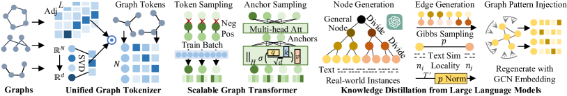
Figure 1. Overall architecture of the OpenGraph. i) A unified graph tokenizer efficiently converts any input graph into universal graph tokens, accommodating variations in node token sets. ii) The scalable graph transformer effectively captures global node-wise dependencies using anchor sampling and efficient self-attention mechanisms. iii) LLM-enhanced data augmentation techniques are employed for synthetic graph generation, addressing the issue of limited domain-specific data availability.

3.1. Unified Graph Tokenizer

To overcome the challenges presented by diverse graphs that differ significantly in terms of nodes, edges, and feature semantics, our primary goal is to develop a graph tokenizer that effectively transforms input graphs into unified token sequences. In our graph tokenizer, each token represents a node and is accompanied by a semantic vector denoted as $\mathcal{G}\rightarrow{\textbf{e}_{0},\textbf{e}_{1},\cdots,\textbf{e}_{|\mathcal{V}|}}$. By utilizing a shared node representation space and employing a flexible sequence data structure, we aim to standardize the distribution of nodes across different graphs. Additionally, we merge the edge information into the unified node representations, disregarding differences between graphs. To address the variations in node features, we introduce a topological representation space that is generated through a consistent mapping procedure.

3.1.1. Smoothed High-Order Adjacency Matrix

In our OpenGraph model, we employ a unified graph tokenizer that utilizes the smoothed adjacency matrix, denoted as $\tilde{\textbf{A}}$, and a topology-aware projection function $\phi:\mathbb{R}^{|\mathcal{V}|}\rightarrow\mathbb{R}^{d}$. This tokenizer is responsible for handling the specific graph representation. To achieve this, we start with the original adjacency matrix $\textbf{A}\in\mathbb{R}^{|\mathcal{V}|\times|\mathcal{V}|}$ constructed from the edges $\mathcal{E}$. In our OpenGraph paradigm, the smoothing procedure for the adjacency matrix is carried out as follows:

(3) $$\tilde{\textbf{A}}=\bar{\textbf{A}}^{1}+\bar{\textbf{A}}^{2}+\cdots\bar{\textbf{A}}^{L},\leavevmode\nobreak\ \leavevmode\nobreak\ \leavevmode\nobreak\ \leavevmode\nobreak\ \leavevmode\nobreak\ \bar{\textbf{A}}=\textbf{D}^{-1/2}\textbf{A}\textbf{D}^{-1/2}$$

Here, we utilize the diagonal degree matrix D derived from the adjacency matrix A. It records the node degree of $v_{i}$ with $d_{i,i}$, and $d_{i,j}=0$ for $i\neq j$. With matrix D, we employ the Laplacian normalization $\bar{\textbf{A}}$ of A to ensure numerical stability. To capture high-order connectivity and address sparsely-observed node-wise relations, our OpenGraph combines the power of $\bar{\textbf{A}}$ at different orders. This allows us to obtain topology information $\tilde{\textbf{A}}$ for further processing, with $L$ representing the maximum power order considered.

3.1.2. Topology-aware Projection with Arbitary Graphs

To handle the significant variability in the dimensions of adjacent matrix $\tilde{\textbf{A}}$ across different graph datasets, using a fixed-input-dimension random neural network is not feasible. To address this challenge, we propose a topology-aware projection approach using a function $\phi:\mathbb{R}^{|\mathcal{V}|}\rightarrow\mathbb{R}^{d}$. By eliminating one of the varying dimensions, we aim to reduce information loss during dimension reduction. To achieve this, we employ a large hidden dimensionality $d$. Prior research (shen2021powerful, ; zheng2022instant, ) has demonstrated that even random projections can yield satisfactory performance when utilizing a large dimensionality. Hence, to better preserve graph information and minimize randomness in our graph tokenizer, we utilize the fast singular value decomposition (SVD) for the projection function $\phi$. Empirical analysis reveals that two iterations of fast SVD effectively preserve topology information while incurring negligible computational overhead. Formally, our graph tokenizer calculates the resulting token sequence based on the following operations:

(4) $$\textbf{e}_{v}=\phi(\tilde{\textbf{A}}_{v,:})=\tilde{\textbf{A}}_{v,:}\text{LN}((\textbf{U}\sqrt{\Lambda}\leavevmode\nobreak\ \|\leavevmode\nobreak\ \textbf{V}\sqrt{\Lambda})),\leavevmode\nobreak\ \leavevmode\nobreak\ \leavevmode\nobreak\ \textbf{U},\Lambda,\textbf{V}=\text{SVD}(\bar{\textbf{A}})$$

The topology-aware projection, obtained through SVD, consists of $\textbf{U},\textbf{V}\in\mathbb{R}^{|\mathcal{V}|\times d}$ and $\Lambda\in\mathbb{R}^{d\times d}$. The concatenation operator $\|$ combines them in the hidden dimension. Layer normalization function $\text{LN}(\cdot)$ reduces numerical variance across datasets. The resulting $\textbf{e}_{v}\in\mathbb{R}^{d}$ incorporates topology information from $\tilde{\textbf{A}}$ and the topology-aware projection $\phi$. This information strengthens subsequent learnable neural networks.

It is worth emphasizing that our graph tokenizer is designed to handle arbitrary variable-sized graphs that undergo significant shifts in terms of node token sets and relational semantics.

3.2. Scalable Graph Transformer

After acquiring the universal topology-aware tokens for all nodes, regardless of any variations in characteristics across diverse graphs, through our unified graph tokenizer, the subsequent task is to empower our graph model to grasp the complex node-wise dependencies within the global context. Drawing inspiration from the success of transformer architectures in modeling complex relationships between instances, our OpenGraph utilizes a graph transformer as the backbone to incorporate global dependencies among all nodes.

To ensure scalability and effectively handle large-scale graph datasets, we introduce the following techniques, to enhance the efficiency of our graph transformer backbone in our OpenGraph.

3.2.1. Token Sequence Sampling

To optimize the efficiency of our model, given the large embedding size, our graph transformer is trained using sampled token sequences from the current training batch. Specifically, the training batch $\{(v_{c_{b}},v_{p_{b}},v_{n_{b}})|b=1,\cdots,B\}$ consists of $B$ triplets of centric nodes $v_{c_{b}}$, positive nodes $v_{p_{b}}$, and negative nodes $v_{n_{b}}$, which serve as input for our graph transformer.

(5) $$(\textbf{e}_{c_{1}},\textbf{e}_{c_{2}},\cdots\textbf{e}_{c_{B}})\leavevmode\nobreak\ \|\leavevmode\nobreak\ (\textbf{e}_{p_{1}},\textbf{e}_{p_{2}},\cdots,\textbf{e}_{p_{B}})\leavevmode\nobreak\ \|\leavevmode\nobreak\ (\textbf{e}_{n_{1}},\textbf{e}_{n_{2}},\cdots,\textbf{e}_{n_{B}})$$

The initial token embeddings ${\textbf{e}_{v}}$ effectively capture the local structural information for each node $v\in\mathcal{V}$. By using the sampled token sequence, we can preserve the graph context with a particular emphasis on the training batch. This approach significantly reduces the sequence length from $|\mathcal{V}|$ to $3\times B$, enabling efficient training for large-scale graphs. Additionally, since the initial token embeddings $\textbf{e}_{v}$ inherently encode the topological closeness among nodes, our graph transformer does not rely on temporal embeddings typically used in transformers for temporal or textual sequences.

3.2.2. Efficient Self-attention with Anchor Sampling

Though sequence sampling reduces the length of the node sequence, the pairwise relation learning in self-attention still exhibits a complexity of $\mathcal{O}(B^{2}\times d)$, which can limit the batch size $B$ required for computational efficiency. To address this challenge, we introduce an additional step of sampling a set of anchor nodes ${v_{a_{s}}}$, where $s=1,\cdots,S$, during the self-attention calculation. Here, $S$ is chosen to be $d/H<B$ to ensure that the self-attention module incurs similar memory costs as other fully-connected components. Here, $H$ represents the number of attention heads. More specifically, the self-attention process for each head can be summarized as follows:

$$\textbf{e}_{t}^{(3)} =\sum_{v_{a}}\alpha_{t,a}\textbf{W}^{(v)}\textbf{e}_{a}^{(2)},\leavevmode\nobreak\ \leavevmode\nobreak\ \leavevmode\nobreak\ \textbf{e}_{a}^{(2)}=\sum_{v_{t}}\alpha_{a,t}\textbf{W}^{(v)}\textbf{e}_{t}^{(1)}$$

(6) $$\alpha_{t,a} =\text{softmax}\Big{(}(\textbf{W}^{(q)}\textbf{e}_{t})^{\top}\cdot(\textbf{W}^{(k)}\textbf{e}_{a})\leavevmode\nobreak\ /\leavevmode\nobreak\ \sqrt{d/H}\Big{)}$$

Our efficient self-attention involves embeddings $\textbf{e}_{*}^{(1)},\textbf{e}_{*}^{(2)},\textbf{e}_{*}^{(3)}$ for anchor nodes $v_{a}$ and vanilla nodes $v_{t}$. After each attention calculation, the results from multiple heads are concatenated, passed through a learnable linear layer, and connected with a residual connection. The parameters $\textbf{W}^{(q)},\textbf{W}^{(k)},\textbf{W}^{(v)}$ are the parameters of the attention layer. To reduce computational complexity, we employ a two-stage self-attention process. It transforms the $3\times B$-length sequence to a shorter $S$-length sequence and then reverses the process. This decomposition reduces the complexity from $\mathcal{O}(B^{2}\times d)$ to $\mathcal{O}(B\times S)$, ensuring scalability for large-scale models.

After the self-attention module, each layer of our scalable graph transformer includes a two-layer fully-connected block with residual connections, accompanied by two layer normalization modules. To ensure numerical stability, per-layer scaling is applied. For a more comprehensive understanding of the specific configurations of our scalable graph transformer, please refer to Appendix A.

3.3. Knowledge Distillation from LLM

Obtaining diverse graph datasets for different domains can be challenging due to factors like privacy issues that restrict access to essential data (zheleva2007preserving, ). Inspired by the remarkable knowledge and understanding demonstrated by large language models (LLMs), we leverage their power to enhance the generation of diverse graph-structured data. To improve the efficacy of our LLM-augmented graph data for pre-training our model, we have developed an augmentation mechanism. This mechanism enables the LLM-augmented graph data to closely approximate real-world graph characteristics, enhancing the relevance and usefulness of the augmented data.

3.3.1. LLM-based Node Generation

When generating graphs, our initial step is to create a node set tailored to the specific application scenario. Each node is characterized by a text-based profile that assists in generating subsequent edges. However, this task can be particularly challenging when dealing with real-world scenarios due to the substantial scale of the node set. For instance, in e-commerce platforms, the graph data may consist of billions of products. As a result, efficiently enabling the LLM to generate a large number of nodes becomes a significant challenge.

To address the above challenge, we employ a strategy that involves iteratively dividing general nodes into sub-categories with finer semantic granularity. For example, when generating product nodes, we begin by prompting the LLM with a query like "List all sub-categories of products on an e-commerce platform like Amazon." The LLM responds with a list of sub-categories such as "clothing," "home & kitchen," "electronics," and so on. We then continue this iterative division process by asking the LLM to further refine each sub-category. This process is repeated until we obtain nodes that closely resemble real-world instances, such as a product with labels like "clothing," "women’s clothing," "sweaters," "hooded sweaters," "white hooded sweaters." Appendix A.3.1 provides more details about our prompt template and specific generation examples.

Tree-of-Prompt Algorithm. The process of dividing nodes into sub-categories and generating fine-grained entities follows a tree structure. The initial general node (e.g., "products," "deep learning papers") serves as the root, and fine-grained entities act as leaf nodes. We employ a tree-of-prompt strategy to traverse and generate these nodes. For further details, please see Appendix A.3.2.

3.3.2. LLM-based Edge Generation by Gibbs Sampling

To generate edges, we use the Gibbs sampling algorithm (gelfand2000gibbs, ) with the generated node set $\mathcal{V}$. The algorithm starts with a random sample, which varies depending on the type of entity-entity relation data. For instance, in a paper-wise citation network, the sample is a node pair $(v_{s_{0}},v_{t_{0}})$. In a person-entity relation scenario like an author-paper or user-item recommendation network, the initial sample is a binary vector $\textbf{a}^{0}\in\{0,1\}^{|\mathcal{V}|}$. Each element $a_{i}=1$ indicates interaction between the sampled person and the $i$-th node $v_{i}$, while $a_{i}=0$ indicates no interaction. In the case of person-entity relations, the Gibbs algorithm for edge sampling is described in Appendix A.3.3. The key is estimating the probability $p(\mathbf{a}^{t}\oplus v_{t^{\prime}}|\mathbf{a}^{t})$, with $\oplus$ representing setting the $t^{\prime}$-th dimension of $\textbf{a}^{t}$ to 1.

Node-wise Connection Probability Estimation. To accurately estimate the probability $p(\mathbf{a}^{t}\oplus v_{t^{\prime}}|\mathbf{a}^{t})$ of connecting two nodes in our generated graph, we leverage the reasoning capabilities of the LLM. However, directly prompting the LLM for predictions on each edge can be computationally expensive, with the number of required prompts scaling proportionally to the number of edges ($\mathcal{O}(|\mathcal{V}|\times|\mathcal{V}|)$). To ensure efficient probability estimation, we adopt an alternative approach. We prompt the LLM to generate hidden representations $\mathbf{h}_{i}$ for each node $v_{i}$. Then, we calculate the relationship between each edge using dot-product similarity as:

(7) $$p(\textbf{a}^{t}\oplus v_{t^{\prime}}|\textbf{a}^{t})=\sum_{v_{i}}a^{t}_{i}(\textbf{h}_{i}/\|\textbf{a}^{t}\|_{0})^{\top}\cdot\textbf{h}_{t^{\prime}}$$

By utilizing the text embeddings $\textbf{h}_{i}$ and $\textbf{h}_{t^{\prime}}$ provided by the LLM, which are in the same representation space, we can effectively capture the semantic relations between the respective nodes.

Dynamic Probability Normalization. To ensure that the calculated probability scores fall within the range of $[0,1]$, our generation algorithm incorporates a dynamic probability normalization approach, which enhances the algorithm’s realism by mimicking real-world distributions. It maintains a record of the most recent $T^{\prime}$ estimation values, denoted as $\mathcal{P}=\{p(\textbf{a}^{t}\oplus v_{t^{\prime}}|\textbf{a}^{t})\leavevmode\nobreak\ |\leavevmode\nobreak\ t=-1,-2,\cdots,-T^{\prime}\}$. By calculating the mean ($\mu$) and standard deviation ($\sigma$) of these values, we obtain an understanding of their distribution. To adjust new estimations, we use $\mu+2\sigma$ as the upper bound and $\mu-2\sigma$ as the lower bound. The resulting adjusted probability score, denoted as $\bar{p}$, is obtained by $\bar{p}=(p-\mu)/(4\sigma)$. Through this normalization process, we ensure that the probability scores are constrained within a range that closely approximates $[0,1]$.

Node Locality Incorporation. Our LLM-based edge generation method effectively determines potential connections based on the semantic similarity between nodes. However, it tends to create excessive connections among all semantically-related nodes, overlooking the important concept of locality observed in real-world graphs. In reality, nodes are more likely to be connected to a subset of relevant nodes, as they have limited interactions with only a portion of all other nodes. To address this, we introduce a way to incorporate the notion of locality in our edge generation process. Each node $v_{i}$ is randomly assigned a locality index $n_{i}$. To account for the difference in locality between two nodes, we use the absolute difference $|n_{i}-n_{j}|$ in an exponential decay function applied to the normalized probability. This results in an adjusted probability $\hat{p}$ calculated as $\hat{p}=\bar{p}\cdot\alpha^{|n_{i}-n_{j}|}$, where $0<\alpha<1$.

3.3.3. Graph Topological Pattern Injection

To enhance the incorporation of topological information in the graph generation process, we refine the node embeddings after the initial graph generation. By training a Graph Convolutional Network (GCN) on the graph $\mathcal{G}$, we obtain new node embeddings that capture the underlying topology patterns. This aligns the node embeddings derived from the graph with the textual embeddings of the entities and avoids distribution shifts between graph and textual spaces. The final graph is constructed using our edge generation algorithm, which operates on these enhanced node representations.

4. Evaluation

Our experiments aim to address the following research questions:

• RQ1: How does OpenGraph compare to existing graph models in zero-shot link prediction and node classification tasks?
  

• RQ2: How does different training datasets (real data and generated data) affect the model performance of OpenGraph?
  

• RQ3: What is the influence of different types of initial graph projection methods on our OpenGraph framework?
  

• RQ4: How does the sampling strategies in our scalable graph transformer impact the model efficiency and performance?
  

• RQ5: How does model scale impact our OpenGraph?
  

• RQ6: How does our OpenGraph perform relative to baseline methods in standard full-shot training and few-shot training?

4.1. Experimental Settings

4.1.1. Datasets

We evaluate our OpenGraph on two graph learning tasks: link prediction and node classification, using a total of 8 real-world datasets. Appendix A.2.1 provides detailed descriptions.

4.1.2. Evaluation Protocol

Following previous works (he2020lightgcn, ; kipf2016semi, ), we adopt the original train-test data split for the experimental datasets. We pre-train our OpenGraph on generated datasets and conducts zero-shot prediction for the evaluation datasets made of real graph data. As most baselines struggle with cross-dataset transferring, we evaluate them in two few-shot training settings. Please refer to Appendix A.2.2 for more details about our cross-dataset zero-shot setting, few-shot settings, and evaluation metrics.

4.1.3. Implementation Details

We provide detailed information about the implementation of OpenGraph and the baseline methods, as well as the graph generation process, in Appendix A.2.3.

Table 1. Performance comparison between our OpenGraph (zero-shot) and baseline methods (one-shot, five-shot) on the link prediction task (measured by Recall@N for $N=20,40$) and node classification task (measured by Accuracy and Macro F1 Score).

Dataset		ogbl-ddi		ogbl-collab		ML-1M		ML-10M		Amazon-book		Cora		Citeseer		Pubmed
Metric		R@20	R@40	R@20	R@40	R@20	R@40	R@20	R@40	R@20	R@40	Acc	MacF1	Acc	MacF1	Acc	MacF1
MF	1-shot	0.0087	0.0161	0.0261	0.0349	0.0331	0.0604	0.1396	0.1956	0.0034	0.0043	0.1710	0.1563	0.1740	0.1727	0.3470	0.3346
	5-shot	0.0536	0.0884	0.0412	0.0609	0.0987	0.1584	0.2060	0.2989	0.0196	0.0284	0.1500	0.1422	0.1520	0.1484	0.3540	0.3435
MLP	1-shot	0.0195	0.0336	0.0112	0.0185	0.0548	0.1019	0.1492	0.2048	0.0017	0.0028	0.2300	0.1100	0.2590	0.1993	0.4430	0.3114
	5-shot	0.0621	0.1038	0.0115	0.0185	0.0851	0.1470	0.2362	0.2563	0.0092	0.0152	0.3930	0.3367	0.3690	0.3032	0.5240	0.4767
GCN	1-shot	0.0279	0.0459	0.0206	0.0321	0.0432	0.0849	0.1760	0.2086	0.0096	0.0160	0.3180	0.1643	0.3200	0.2096	0.4270	0.3296
	5-shot	0.0705	0.1312	0.0366	0.0513	0.1054	0.1656	0.2127	0.2324	0.0251	0.0408	0.5470	0.5008	0.4910	0.4190	0.509	0.4455
GAT	1-shot	0.0580	0.1061	0.0258	0.0372	0.0245	0.0520	0.1615	0.2476	0.0047	0.0079	0.2420	0.1687	0.2810	0.2025	0.4720	0.3657
	5-shot	0.0711	0.1309	0.0340	0.0505	0.1506	0.2267	0.2002	0.2883	0.0228	0.0392	0.585	0.5438	0.4940	0.4441	0.5780	0.5582
GIN	1-shot	0.0530	0.1004	0.0163	0.0247	0.0466	0.0884	0.1541	0.2388	0.0069	0.0114	0.3190	0.1753	0.2820	0.1705	0.4410	0.3064
	5-shot	0.0735	0.1441	0.0311	0.0458	0.1458	0.2344	0.1926	0.2829	0.0252	0.0418	0.5400	0.4941	0.521	0.4696	0.5070	0.4547
DGI	1-shot	0.0315	0.0617	0.0255	0.0385	0.0486	0.0863	0.1868	0.2716	0.0081	0.0142	0.3150	0.1782	0.2840	0.1791	0.4290	0.3163
	5-shot	0.0821	0.1426	0.0345	0.0502	0.1687	0.2573	0.2303	0.3063	0.0300	0.0492	0.4880	0.4606	0.4450	0.4062	0.4890	0.4509
GPF	1-shot	0.0503	0.0856	0.0027	0.0048	0.1099	0.1702	0.1599	0.2326	0.0072	0.0128	0.3080	0.1952	0.3110	0.1984	0.4220	0.2670
	5-shot	0.0839	0.1460	0.0027	0.0047	0.0817	0.1392	0.2014	0.2994	0.0179	0.0310	0.5550	0.5233	0.4690	0.4223	0.5150	0.4934
GPrompt	1-shot	0.0541	0.1102	0.0138	0.0207	0.0797	0.1310	0.1362	0.2073	0.0074	0.0120	0.3540	0.1596	0.2800	0.1519	0.4710	0.3705
	5-shot	0.0769	0.1396	0.0157	0.0231	0.1340	0.2166	0.2157	0.3147	0.0287	0.0464	0.5510	0.5098	0.5570	0.5211	0.5130	0.4520
GraphCL	1-shot	0.0603	0.1112	0.0265	0.0398	0.0390	0.0799	0.1655	0.2529	0.0047	0.0077	0.2430	0.1548	0.2980	0.1630	0.4070	0.4130
	5-shot	0.0740	0.1368	0.0311	0.0456	0.1416	0.2138	0.2019	0.3075	0.0270	0.0440	0.5610	0.5330	0.4300	0.3683	0.5230	0.5024
OpenGraph	0-shot	0.0921	0.1746	0.0421	0.0639	0.1911	0.2978	0.2370	0.3265	0.0485	0.0748	0.7504	0.7426	0.6097	0.5821	0.6869	0.6537

4.1.4. Baselines

Our empirical evaluation utilizes the following 9 state-of-the-art baseline methods from 4 different research lines. Detailed descriptions for the baselines can be found in Appendix A.2.4.

4.2. Overall Performance Comparison (RQ1)

We begin by comparing the zero-shot performance of OpenGraph with the few-shot performance of the baselines in both link prediction and node classification. The results are displayed in Table 1. Based on these results, we have made the following observations:

O1: Predominant Performance of OpenGraph. Our model demonstrates superior performance across all 8 datasets in various categories. Notably, this advantage is achieved solely through pre-training on a generated dataset, without any overlap with the downstream graph data. This highlights the remarkable ability of our model to generalize across different datasets. We attribute this advantage to three key factors: i) The unified graph tokenizer, which effectively bridges the distribution gap between the pre-training and target datasets. ii) The scalable graph transformer, which excels at learning relations and capturing important structural features, resulting in high-quality graph representations. iii) The effective pre-training with LLM-generated graph data, which equips our model with versatile forecasting abilities for unseen downstream datasets. Overall, these design choices contribute to the outstanding generalization capabilities of our model across diverse datasets.

O2: Limitations of Existing Pretraining Methods. Observations reveal that pre-training techniques, such as GraphCL and DGI, do not consistently surpass their foundational models, like GIN and GCN, which were trained solely on few-shot data. This pattern suggests that the pre-training methods may hinder rather than help performance when models are applied to different datasets. Such underperformance is likely due to a substantial shift in data distribution between the pre-training and target datasets, which can lead the model to become overfitted to the pre-training data, thus impairing its ability to adapt to new graph structures in the downstream tasks. Furthermore, prompt tuning methods like GraphPrompt and GPF sometimes degrade more severely compared to full-model fine-tuning approaches, which indicates an even greater susceptibility to overfitting to distinctive patterns within the pre-training dataset.

O3: Tackling Node Classification by Structure Learning. Our OpenGraph exhibits a marked improvement in node classification tasks, which underscores the efficacy of employing our pre-trained link predictor to discern the connections between ordinary nodes and special nodes representing classes. This advantage hinges on OpenGraph’s robust capacity to generalize, as it successfully transfers knowledge both across different datasets and between distinct tasks. The credit for this versatility goes to the universal applicability and flexibility of our graph tokenization and graph encoding.

4.3. Investigation on Graph Tokenizer (RQ2)

In this section, we study the effectiveness of our unified graph tokenization module. This investigation involves an evaluation of the impact of the smoothed adjacency matrix and a comparison of our topology-aware projection method with alternative compression methods. The evaluation results are presented in Figure 2, based on which we make the following analysis.

Impact of adjacency smoothing: We examine the effect of graph smoothing on model performance by testing different levels of smoothing for the input adjacency matrix. The results are depicted in Figure 2(a) and 2(b). Here, the use of 0 adjacency smoothing implies the input of an identity matrix for the graph tokenizer. This approach significantly damages the topological information for the graph tokenizer, resulting in poor performance. This outcome underscores the importance of considering the adjacency matrix within our unified graph tokenizer. For the non-zero graph smoothing orders, $L=2$ produces the best performance for the Movielens-1M dataset. $L=3$ and $1$ yield the best performance for the OGBL-ddi data under the top-20 and top-40 settings, respectively. This suggests the benefits of exploring high-order graph smoothing in the graph tokenizer of our OpenGraph.

Superiority of topology-aware projection. To assess the effectiveness of our topology-aware projection based on fast SVD, we compare it to three alternative projection modules (see Appendix A.2.5 for more details). The results are presented in Figure 2(c) and 2(d). We make the following observations:

• One-hot encoding. This graph projection strategy learns id-corresponding embeddings across datasets. It performs poorly in our zero-shot evaluation, highlighting the difficulty of transferring dataset-specific parameters such as node embeddings to unseen datasets that lack overlapping node tokens.
  

• Degree embeddings. This method learns degree-specific embeddings. It demonstrates a significant performance disadvantage compared to our projection scheme. This can be attributed to the substantial semantic gap that exists for the same degree number across different graphs. Additionally, this approach oversimplifies the topology features by considering only the number of direct links, which limits its ability to capture more nuanced structural patterns and can be detrimental to the graph projection.
  

• Random projection. It randomly assigns an unlearnable embedding vector to each node. The results demonstrates its advantages over the other two variants. However, due to the low representation efficiency of its uniform distribution, this method also exhibits poorer performance compared to our method.

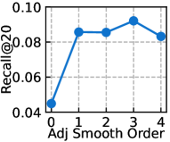
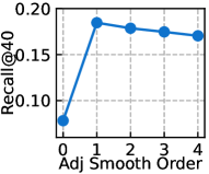
(a) OGBL-ddi dataset.

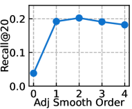
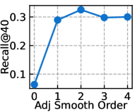
(b) Movielens-1M dataset.

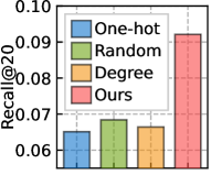
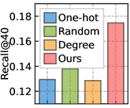
(c) OGBL-ddi dataset.

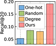
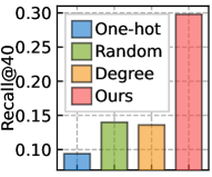
(d) Movielens-1M dataset.

Figure 2. Influence of graph tokenizer configurations.

4.4. Influence of Pre-training Datasets (RQ3)

To evaluate the effectiveness of our knowledge distillation from the LLM, we compare the performance of OpenGraph networks that are pre-trained with different datasets. In our experiments, we employ three ablated versions of our graph generation algorithm, namely -Norm, -Loc, and -Topo (further details below). Additionally, we incorporate two real datasets, Yelp2018 and Gowalla, for pre-training, which are unrelated to the test datasets used in this experiment. Moreover, we include the ML-10M dataset, which is related to both ML-1M and itself, in the test datasets. The evaluation results are summarized in Table 2. We draw the following conclusions:

Superiority of our generated data. Our generated dataset, referred to as Gen, achieves the best performance on all test datasets except for ML-1M and ML-10M. Notably, ML-10M, which is closely related to these two datasets, achieves the best performance in these cases. This finding highlights the superior generalization ability of our generated datasets, which equips the OpenGraph model with the capability of universal topological structure learning.

Effectiveness of individual generation techniques. We conduct ablation study by removing the dynamic probability normalization (-Norm), locality incorporation (-Loc), and graph topological pattern injection (-Topo) modules. The removal of these modules from the graph generation algorithm leads to a significant drop in performance for the downstream prediction. This demonstrates the effectiveness of these three key modules for our generated graphs.

Real-world data can be misleading. Using real-world datasets such as Yelp2018 and Gowalla does not yield transferable graph learning capabilities that provide an advantage over our Gen dataset. This highlights the limitation of relying solely on insufficient or biased real-world data for cross-dataset pre-training.

Pretraining on related datasets is useful. Models pre-trained on ML-10M exhibit superior performance on ML-1M and ML-10M, which are directly related datasets. This indicates that dataset-wise similarity can aid in the cross-dataset knowledge transferring.

Table 2. Influence of utilizing different pre-training datasets.

Test	Pre-training Dataset
Dataset	-Norm	-Loc	-Topo	Yelp2018	Gowalla	ML-10M	Gen
ogbl-ddi	0.0737	0.0893	0.0656	0.0588	0.0770	0.0692	0.0921
ML-1M	0.0572	0.1680	0.0850	0.0599	0.0485	0.2030	0.1911
ML-10M	0.0982	0.1636	0.1017	0.1629	0.0910	0.2698	0.2370
Cora	0.4985	0.4864	0.4342	0.3715	0.5943	0.2780	0.7504
Citeseer	0.3944	0.3691	0.5743	0.2651	0.4300	0.2003	0.6097
Pubmed	0.4501	0.5015	0.4876	0.3317	0.5148	0.3652	0.6869

4.5. Impact of Sampling in Transformer (RQ4)

We examine the influence of token sequence sampling and anchor sampling in our scalable graph transformer architecture. The metrics for efficiency and performance are summarized in Table 3. Our evaluation focuses on the GPU memory costs and the running time during both the training and testing processes. The OGBL-ddi and ML-10M datasets are used for evaluation. Additionally, we assess the model performance after end-to-end training on these datasets. The following observations are made for the ablated versions.

• -Seq-Anc: This variant eliminates both token sequence sampling and anchor sampling, leading to out-of-memory (OOM) errors when applied to the larger ML-10M dataset. In the evaluation on OGBL-ddi, it exhibits the lowest memory and time efficiency, while its performance is inferior to our OpenGraph model.
  

• -Anc: This version incorporates only sequence sampling into the graph transformer. It significantly reduces memory costs during the training phase. Additionally, by focusing on the current training context, it achieves the best performance on OGBL-ddi.
  

• -Seq: This model removes token sequence sampling from our OpenGraph architecture, resulting in a significant decrease in training efficiency. However, the anchor sampling strategy in this version greatly reduces computational costs during the test phase. Despite the computational benefits, the anchor sampling strategy leads to a drop in performance compared to our OpenGraph.

Table 3. Impact of sampling strategies on the efficiency and model performance in the scalable graph transformer.

OGBL-ddi	Train Mem	Test Mem	Train Time	Test Time	Recall@20
-Seq-Anc	5420MiB	1456MiB	22.72s	13.88s	0.0966
-Anc	3360MiB	1456MiB	18.19s	13.73s	0.1107
-Seq	2456MiB	1202MiB	16.45s	12.09s	0.0930
OpenGraph	2358MiB	1202MiB	15.45s	12.09s	0.1006
ML-10M	Train Mem	Test Mem	Train Time	Test Time	Recall@20
-Seq-Anc	OOM	OOM	–	–	–
-Anc	4996MiB	OOM	73.15s	–	–
-Seq	23140MiB	4550MiB	158.60s	84.78s	0.2772
OpenGraph	4470MiB	4550MiB	68.79s	54.17s	0.2816

4.6. Impact of Model Scale (RQ5)

This section examines the influence of model scale within our OpenGraph framework. Specifically, we modify two crucial hyperparameters that significantly impact the scale of learnable parameters: the number of graph transformer layers $L^{\prime}$, and the hidden dimensionality $d$. We assess the model’s performance on the link prediction task by measuring Recall@20. Additionally, we evaluate the computational time for 100 training steps and 100 test steps. The results are illustrated in Figure 3. We summarize the key findings as follows:

Number of graph transformer layers. It can be observed that both training and testing time of OpenGraph exhibit a linear increase as the number of graph transformer layers grows. However, the expansion in model size does not consistently lead to performance improvement. The lack of performance enhancement can be attributed to the overfitting effect and the increased training complexity associated with deep transformer networks.

Hidden dimensionality. In contrast to the number of graph transformer layers, the hidden dimensionality leads to quadratic growth in computational time. This reflects the rapid increase in model capacity required to accommodate more complex structural data. Consequently, we observe significant improvements in model performance, surpassing the performance curve for the graph transformer layers. Despite the increased model capacity, the growth in hidden dimensionality facilitates the $\mathbb{R}^{N}\rightarrow\mathbb{R}^{d}$ projection, reducing information loss and enhancing the quality of the graph token sequence for the subsequent graph transformer layers.

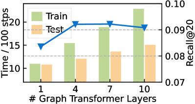
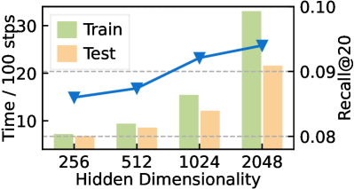
(a) Performance and time change on the OGBL-ddi dataset.

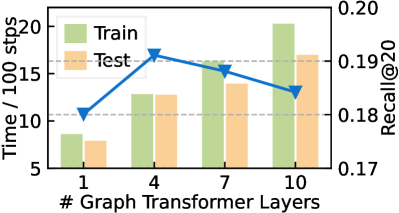
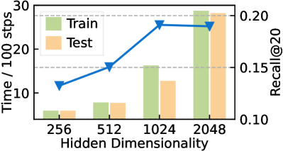
(b) Performance and time change on the ML-1M dataset.

Figure 3. The impact of OpenGraph model scale on downstream data performance and training/testing time (seconds).

4.7. End-to-End Training Performance (RQ6)

To assess the modeling capabilities of our OpenGraph framework, we perform a performance comparison between OpenGraph and the baselines trained on the same few-shot datasets. Due to space limitations, we present the detailed results and analysis in Appendix A.2.6. The results demonstrate strong graph learning capabilities of our OpenGraph, even in the supervised learning settting.

5. Related Work

Graph Neural Networks. Graph Neural Networks (GNNs) have gained significant attention in recent years due to their ability to effectively capture and model complex relationships within graph-structured data (wu2020comprehensive, ; zhang2022graph, ; chen2020simple, ). GNNs utilize message passing schemes to propagate information across the graph and aggregate information from the neighboring nodes for node representations (jin2021universal, ; yuan2020xgnn, ). Several representative graph neural architectures have been developed. For example, Graph Convolutional Networks (GCNs) adapt the concept of convolution to operate on graph-structured data and enable nodes to exchange messages with their neighbors (gao2018large, ; zhang2021lorentzian, ). Additionally, Graph Attention Networks (GANs) are introduced to address the limitations of traditional GCNs in capturing complex relationships and varying importance levels between nodes in a graph (zhang2022graph, ; liao2019efficient, ). The backbone of OpenGraph draws inspiration from the powerful Graph Transformer (yun2019graph, ; hu2020heterogeneous, ) in capturing long-range dependencies and global information in graphs.

Self-Supervised Learning on Graphs. To tackle the issue of limited labeled data in graph tasks, self-supervised graph learning techniques, such as contrastive and generative approaches, provide promising solutions (wu2021selftkde, ; lee2022augmentation, ; xia2023automated, ). These methods leverage the inherent structure and patterns within graphs to train models in a data-efficient manner (xiao2022decoupled, ; yang2023graph, ). Specifically, graph contrastive learning frameworks focus on creating meaningful representations by contrasting positive and negative samples. Notable models in this area include GraphCL (you2020graph, ) and SGL (wu2021self, ), which utilize stochastic data augmenters. Additionally, adaptive augmentation schemes such as JOAO (you2021graph, ) and GCA (zhu2021graph, ) have been proposed. Another paradigms, DGCL (li2021disentangled, ) and UMGRL (mo2023disentangled, ), addresses the challenge of disentangling factors within contrastive learning. However, existing solutions often struggle to generalize well across diverse downstream graph scenarios due to their strong assumptions of a consistent graph token set. This work proposes OpenGraph, which enhances graph model generalization across different graph tasks.

LLM-based Methods for Graph Analysis. Recent advancements in the field of large language models (LLMs) have sparked researchers’ interest in leveraging their potential to enhance graph comprehension and analysis (chai2023graphllm, ; fatemi2023talk, ; ren2023representation, ; guo2024graphedit, ). Notably, GraphLLM (chai2023graphllm, ) and GraphQA (fatemi2023talk, ) are notable examples of efforts aimed at transforming graphs into natural language descriptions. Leveraging such descriptions as inputs for LLMs enables improved interpretation and reasoning on graph data. Additionally, techniques like instruction tuning in GraphEdit (guo2024graphedit, ) and GraphGPT (tang2023graphgpt, ) facilitate fine-tuning LLMs by incorporating rich textual information from text-attributed graphs. However, the success of these methods heavily relies on the availability of high-quality textual features associated with graph nodes. Acquiring such features can be challenging in certain graph domains. For example, privacy concerns can hinder obtaining high-quality text-attributed graphs in user behavior graphs, and constructing comprehensive textual descriptions for neurons in a brain’s neuronal graph can be difficult. Therefore, there is a need to develop a graph model that can capture universal structural patterns from graphs, even in the absence of textual data.

6. Conclusion

The main focus of this research is to develop a highly adaptable framework capable of accurately capturing and comprehending the intricate topological patterns found in diverse graph structures. By harnessing the potential of the proposed model, our intention is to significantly improve the model’s ability to generalize and perform effectively in zero-shot graph learning tasks encompassing a diverse spectrum of downstream applications. To further improve the efficiency and robustness of OpenGraph, we build our model upon a scalable graph transformer architecture together with a LLM-enhanced data augmentation mechanism. Through extensive experiments conducted on multiple benchmark datasets, we have demonstrated the exceptional generalization abilities of our model. This study makes an initial attempt to exploit the graph fundation model. In future work, our plan is to empower our framework with the capability to automatically discover noisy connections and influential structures with counterfactual learning, while learning the universal and transferable structural patterns of diverse graphs.

Appendix A Appendix

A.1. Model Optimization

To optimize our OpenGraph model, we utilize the masked autoencoding (MAE) training paradigm for self-supervised pre-training. Let’s denote our OpenGraph as $f$, with trainable parameters $\mathbf{\Theta}_{f}$, and a graph projection function $\phi$. The model is trained on a set of graphs $\mathcal{G}_{s}$ with batch-specific labels $\bar{\mathcal{E}}_{s}$. The objective of the generative SSL optimization is defined as follows:

(8) $$\mathop{\arg\min}_{\mathbf{\Theta}_{f}}\sum_{\mathcal{G}_{s}}\sum_{\bar{\mathcal{E}}_{s}\in\mathcal{G}_{s}}\mathcal{L}\Big{(}f(\mathcal{G}_{s}-\bar{\mathcal{E}}_{s},\phi;\mathbf{\Theta}_{f}),\leavevmode\nobreak\ \bar{\mathcal{E}}_{s}\Big{)}+\lambda\|\mathbf{\Theta}_{f}\|_{\text{F}}^{2}$$

Here, $\mathcal{G}_{s}-\bar{\mathcal{E}}_{s}$ represents the input graph $\mathcal{G}_{s}$ with the label edge set $\bar{\mathcal{E}}$ removed. All training graphs $\mathcal{G}_{s}$ are jointly trained with random alternations. To enhance the model’s adaptability to different graph projections $\phi$, we regenerate the projection function $\phi$ for each training graph $\mathcal{G}_{s}$ every 10 training steps. The weight $\lambda$ is used for the parameter decay regularization term.

A.2. Experiments

Table 4. Statistics of experimental datasets.

Dataset		# Nodes	# Edges	# Features	# Classes
Link	OGBL-ddi	4,267	1,334,889	0	N/A
	OGBL-collab	235,868	1,285,465	128
	ML-1M	9,746	720,152	0
	ML-10M	80,555	7,200,040	0
	Amazon-book	144,242	2,380,730	0
Node	Cora	2,708	10,556	1433	7
	Citeseer	3,327	9,104	3,703	6
	Pubmed	19,717	88,648	500	3
Generated	Gen0	46,861	454,276	0	N/A
	Gen1	51,061	268,007	0
	Gen2	32,739	240,500	0

A.2.1. Experimental Datasets

Our experimental datasets include 5 link prediction datasets and 3 node classification datasets. The data statistics are summarized in Table 4.

Link prediction datasets. We employ five link prediction datasets from diverse application scenarios. The objective of these datasets is to predict the most likely connections for each node based on previous observations of node-wise interactions.

• OGBL-ddi. This dataset is used for drug-drug interaction prediction. Each node represents an approved or experimental drug. The edges represent the combined effect of taking two drugs together, which differs significantly from taking them individually.
  

• OGBL-collab. This is an academic social relation dataset. Its nodes represent scholars, and edges denote collaborations. Each node is combined with a 128-dimensional average word embedding calculated from the author’s historical publications.
  

• Movielens-1M & Movielens-10M. These two datasets are collected from the movie rating platform Movielens. The graphs are constructed by connecting users with the movies they have rated. They contain 1 million and 10 million rating records, respectively.
  

• Amazon-book. This dataset contains review data from the Amazon platform. The nodes in the dataset represent users and books, while the edges denote the review records between them.

Node classification datasets. For the node classification task, we utilize three widely-used citation network datasets: Cora, Citeseer, and Pubmed. In these datasets, each node represents an academic paper, and an edge $(v_{i},v_{j})$ denotes a citation relation from paper node $v_{i}$ to $v_{j}$. The Cora and Citeseer datasets include binary bag-of-words vectors as node features, while the Pubmed dataset utilizes TF-IDF weighted word vectors as node features. The objective of these datasets is to classify each node into predefined paper categories based on the citation relations and node attributes.

A.2.2. Evaluation Protocol

This section includes detailed description for our cross-dataset zero-shot setting and the few-shot settings for baselines. It also introduces our evaluation metrics.

Zero-shot setting. For our OpenGraph, we utilize a zero-shot learning setting in which OpenGraph is not trained on any of these real-world datasets but is tested using the training set information as input information, including the graph structures, node features, and node labels in the training set. To effectively generalize to unseen node labels in node classification with zero shot, taking inspiration from previous works [27], we treat the label classes as new nodes and connect the vanilla nodes with training labels to the corresponding class nodes. This strategy removes the requirement for learning class-related parameters in the zero-shot learning setting. This enhancement is also applied to baselines methods.

Few-shot setting. Since most baselines perform poorly in the foregoing zero-shot setting, we evaluate them in the one-shot setting and five-shot setting. In the node classification task, the k-shot setting refers to preserving a maximum of k training instances for each label class. For the link prediction task, the k-shot training set contains at most k links for each node. Non-pretraining approaches such as MLP and GNNs are solely trained on the few-shot training set. On the other hand, baselines following the pretraining-and-tuning paradigm undergo pretraining and subsequent tuning on the few-shot set. In link prediction, they are pretrained on the same generated datasets as our OpenGraph. Model parameters that are not transferable across datasets are re-learned during the tuning phase. In node classification, these methods are pretrained on the graph of the target dataset and fine-tuned on the classification labels. In the test phase, all information in the training set is employed.

Evaluation metrics. In link prediction, we follow existing works [33] to conduct the full-rank test for each node. To be specific, for each node, all nodes not connected to it in the training set are ranked by the model. The top-N nodes are taken as positive predictions, and we calculate Recall@N scores with $N=20,40$. In node classification, we employ the widely-used Accuracy and Macro-F1 metrics [4].

A.2.3. Implementation Details

We implemented our OpenGraph framework using PyTorch. The model employs the Adam optimizer with a learning rate of $1e-4$ or $5e-5$. The learnable parameters are initialized using the Xavier uniform initialization method. By default, the reported performance is achieved by OpenGraph with an embedding size of $d=1024$ and a maximum power order of $L=3$ for adjacency smoothing. The default scalable graph transformer utilizes $L^{\prime}=3$ transformer layers, $H=4$ attention heads, and $S=256$ sampled anchor nodes. The training batch size, which is also used for token sequence sampling, is set as $B=1024$.

The reported results are obtained by pretraining our OpenGraph using three generated datasets: Gen0, Gen1, and Gen2. The statistics of these datasets are presented in Table 4. We first generate the Gen0 dataset without injecting the graph’s topological pattern. Subsequently, we generate Gen1 and Gen2 based on Gen0 by incorporating the graph pattern. In comparison to Gen1, the Gen2 dataset undergoes an additional densification process, where nodes with less than 10 edges are removed. To acquire the nodes for the Gen0 dataset, we prompt the LLM to iterate through all products on an e-commerce platform, with a maximum generation depth of $5$. The Gibbs sampling algorithm is initialized with nodes having $6$ random edges. To ensure low overlap between consecutive samples, we introduce a separation of $1000$ sampling steps before generating each new sample. The dynamic probability normalization maintains the last $T^{\prime}=5000$ sampling instances. The node locality incorporation involves using $7$ locality indices and $0.95$ decay rate.

The baseline methods are evaluated using their original code, or we closely follow the original code to implement them. Our implementations of the baselines are carefully aligned with the reported performance in their original evaluation settings. We employ grid search to optimize the hyperparameter settings for each baseline.

A.2.4. Baselines

We give detailed descriptions for the baseline models in this section. 9 models from 4 categories are utilized.

Graph-agnostic Approaches.

• MF. This is the matrix factorization approach which learns node embeddings to reconstruct the observed adjacency matrix. For the node classification task, we adapt it to learn embedding vectors for each node with the goal of predicting node labels.
  

• MLP. This baseline utilizes a multi-layer perceptron to extract deep features individually for each node. For datasets without node attributes, this baseline learns initial node embeddings.

Non-pretraining Graph Neural Networks.

• GCN [16]. This approach utilizes iterative graph convolutional operators to extract the high-order topological information.
  

• GAT [30]. This graph attention network learns weights for node-wise connections using the attention mechanism, to facilitate adaptive graph information propagation and aggregation.
  

• GIN [40]. This method enhances the representation power of GNNs by employing a distinct graph encoding method that emphasizes the discrimination of non-isomorphic structures.
  

Graph Pre-training Models.

• GraphCL [52]. This baseline method utilizes pre-training of graph models through the application of a self-discriminative contrastive learning task on learned node embeddings. It incorporates various graph augmentation techniques such as node drop, edge permutation, random walk, and feature masking.
  

• DGI [31]. This method introduces a self-supervised pre-training task that aims to maximize the mutual information between the local node view and the global graph view.

Graph Prompt Tuning Methods.

• GraphPrompt [21]. This work presents a unified framework for pre-training and prompt tuning of graph models. It introduces a learnable prompt layer that automatically identifies crucial information in the pre-trained model for downstream tasks.
  

• GPF [5]. This is a universal graph prompt tuning framework designed for various graph pre-training strategies. It introduces two versions of a learnable graph prompt layer.

A.2.5. Alternative Graph Projection Methods (RQ2)

• One-hot encoding. This graph projection strategy employs a large table of low-dimensional embeddings for node ids, where nodes with the same index from different datasets are directly mapped to the same embedding vector. Specifically, we utilize 100,000 independent embedding vectors. For datasets with more nodes, we use the remainder of 100,000 dividing node indices.
  

• Degree embeddings. Degree embeddings are a commonly used node representation strategy for non-attributed graphs. Each degree number is assigned an independent embedding vector, and each node is initially represented by its degree representation.
  

• Random projection. In this approach, a random representation vector is assigned to each node, sampled from a uniform distribution. With a sufficiently large representation space, this method aims to approximately distribute nodes with equal distances from one another. As a result, this projection method does not rely on any specific assumptions about the node distribution. This characteristic allows it to outperform the other two strategies, which are based on certain assumptions and are thus more prone to overfitting the pre-training dataset.

A.2.6. End-to-end Training Performance (RQ6)

Table 5. Performance comparison with models trained on few-shot datasets, in terms of Recall@20 (%).

Dataset	GCN		GAT		GIN		OpenGraph
	1-shot	5-shot	1-shot	5-shot	1-shot	5-shot	1-shot	5-shot
OGBL-ddi	2.79	7.05	5.80	7.11	5.30	7.35	7.93	8.60
ML-1M	4.32	10.54	2.45	15.06	4.66	14.58	16.58	19.19
Amazon-book	0.96	2.51	0.47	2.28	0.69	2.52	2.96	3.10

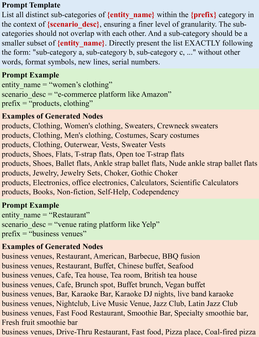
Figure 4. LLM prompt template and generation examples.

We compare our OpenGraph with other graph encoding methods in the supervised learning setting. The models are trained using the 1-shot and 5-shot training sets from OGBL-ddi, ML-1M, and Amazon-book, and then tested on the corresponding test set. Without pre-training, this experiment aims to examine the modeling capacity for different graph neural architectures. From the results shown in Table 5, we draw the following conclusions:

• Superior modeling capabilities of OpenGraph. Our OpenGraph achieves best performance on all tested datasets, demonstrating the superior graph learning ability for OpenGraph. We attribute this superiority to the precise preservation of structural information by our graph tokenization module, and the strength of our scalable graph transformer in learning global relations.
  

• Robustness of OpenGraph. We notice that our OpenGraph exhibits less performance degradation on the more sparse 1-shot datasets. This demonstrates the inherent robustness of OpenGraph’s model architecture. Such robustness can be ascribed to the effectiveness of the fast topology projection, which effectively captures key graph structures even without sufficient training.

A.3. Graph Generation Algorithm

A.3.1. Prompt Template and Generation Examples

In this section, we present our prompt strategy for leveraging the Language Model (LLM) to divide general nodes into more fine-grained entities. Figure 4 illustrates our prompt template, with key parameters highlighted in red. We provide concrete examples of prompt parameters and showcase the generation results for both the e-commerce scenario and the venue rating scenario.

A.3.2. Node Generation Algorithm

We elaborate the process of our tree-of-prompt algorithm that traversing the vertex space for a specific application scenario, as in Algorithm 1.

Input: Name for the initial general node $v_{0}$ (e.g. ’products’), text descriptions for the application scenario $S$ (e.g. ’e-commerce platform like Amazon’), maximum depth $D$ of the prompt tree

Output: Generated nodes $\hat{\mathcal{V}}$.

1

2 Function DivideNode($v$, $n$):

3       if $n\geq D$ then

4            return [$v$]

5       end if

6      

7      $\bar{\mathcal{V}}=\text{LLM}(v,S)$

8       $\hat{\mathcal{V}}=[]$

9       foreach $v^{\prime}\in\bar{\mathcal{V}}$ do

10             $\hat{\mathcal{V}}+=$ DivideNode($v^{\prime}$, $n+1$)

11       end foreach

12      return $\hat{\mathcal{V}}$

13

return DivideNode($v_{0}$, $1$)

Algorithm 1 Node generation based on tree-of-prompt.

A.3.3. Edge Generation Algorithm

We elaborate our edge generation algorithm based on LLM-given node representations and the Gibbs sampling algorithm in Algorithm 2. Here we illustrate the case for generating person-entity relations, which is more complex compared to the entity-entity relation generation.

Input: Node embedding table H given by the LLM, node set $\mathcal{V}$, maximum locality index $N$, locality decay factor $\alpha$, dynamic probability normalization range $T^{\prime}$, number of sampling steps to draw a new sample $T_{0}$, number of initial sampling steps to skip for data quality $T_{1}$, number of sampling steps to shift current locality index $T_{2}$, maximum sampling steps $T_{\text{max}}$.

Output: List of interactions $\mathcal{I}$.

1 Draw a random interaction sample $\textbf{a}^{0}$

2 Initialize current locality index $n=0$

3 Initialize the pool for dynamic probability $\mathcal{P}=[]$

4 Initialize $\mathcal{I}=[]$ for $t=1$ to $T_{\text{max}}$ do

5       if $t\leavevmode\nobreak\ \text{mod}\leavevmode\nobreak\ T_{2}==0$ then

6             $n=(n+1)\leavevmode\nobreak\ \text{mod}\leavevmode\nobreak\ N$

7       end if

8      $i=t\leavevmode\nobreak\ \text{mod}\leavevmode\nobreak\ |\mathcal{V}|$

9       $p=\sum_{v_{i}}a^{t}_{i}(\textbf{h}_{i}/\|\textbf{a}^{t}\|_{0})^{\top}\cdot\textbf{h}_{t^{\prime}}$

10       $\mathcal{P}+=[p]$

11       if $|\mathcal{P}|>T^{\prime}$ then

12             $\mathcal{P}=\mathcal{P}[-T^{\prime}:]$

13       end if

14      $\mu=\text{mean}(\mathcal{P})$, $\sigma=\text{std}(\mathcal{P})$

15       $\bar{p}=(p-\mu)/(4\sigma)$

16       $\hat{p}=\bar{p}\cdot\alpha^{|n-n_{i}|}$

17       Decide if $\textbf{a}^{t}\oplus v_{t^{\prime}}$ is accepted accordding to $\hat{p}$

18       if $t\geq T_{1}$ and $t\leavevmode\nobreak\ \text{mod}\leavevmode\nobreak\ T_{0}==0$ then

19             $\mathcal{I}+=[\textbf{a}^{t}\oplus v_{t^{\prime}}]$

20       end if

21      

22 end for

return $\mathcal{I}$

Algorithm 2 Edge generation based on Gibbs sampling.

References

- [1] Z. Chai, T. Zhang, L. Wu, K. Han, X. Hu, X. Huang, and Y. Yang. Graphllm: Boosting graph reasoning ability of large language model. arXiv preprint arXiv:2310.05845, 2023.
- [2] H. Chen, Z. Wang, F. Huang, X. Huang, Y. Xu, Y. Lin, P. He, and Z. Li. Generative adversarial framework for cold-start item recommendation. In SIGIR, pages 2565–2571, 2022.
- [3] M. Chen, Z. Wei, Z. Huang, B. Ding, and Y. Li. Simple and deep graph convolutional networks. In ICML, pages 1725–1735. PMLR, 2020.
- [4] M. Chen, Z. Zhang, T. Wang, M. Backes, M. Humbert, and Y. Zhang. Graph unlearning. In SIGSAC, pages 499–513, 2022.
- [5] T. Fang, Y. Zhang, Y. Yang, C. Wang, and L. Chen. Universal prompt tuning for graph neural networks. NeurIPS, 2023.
- [6] B. Fatemi, J. Halcrow, and B. Perozzi. Talk like a graph: Encoding graphs for large language models. In NeurIPS 2023 Workshop: New Frontiers in Graph Learning, 2023.
- [7] H. Gao, Z. Wang, and S. Ji. Large-scale learnable graph convolutional networks. In KDD, pages 1416–1424, 2018.
- [8] A. E. Gelfand. Gibbs sampling. Journal of the American statistical Association, 95(452):1300–1304, 2000.
- [9] S. Gui, X. Li, L. Wang, and S. Ji. Good: A graph out-of-distribution benchmark. NeurIPS, 35:2059–2073, 2022.
- [10] Z. Guo, L. Xia, Y. Yu, Y. Wang, Z. Yang, W. Wei, L. Pang, T.-S. Chua, and C. Huang. Graphedit: Large language models for graph structure learning. arXiv preprint arXiv:2402.15183, 2024.
- [11] X. He, K. Deng, X. Wang, Y. Li, Y. Zhang, and M. Wang. Lightgcn: Simplifying and powering graph convolution network for recommendation. In SIGIR, pages 639–648, 2020.
- [12] Z. Hu, Y. Dong, K. Wang, and Y. Sun. Heterogeneous graph transformer. In WWW, pages 2704–2710, 2020.
- [13] D. Jin, Z. Yu, C. Huo, R. Wang, X. Wang, D. He, and J. Han. Universal graph convolutional networks. NeurIPS, 34:10654–10664, 2021.
- [14] W. Jin, X. Liu, X. Zhao, Y. Ma, N. Shah, and J. Tang. Automated self-supervised learning for graphs. In ICLR, 2022.
- [15] W. Jin, Y. Ma, X. Liu, X. Tang, S. Wang, and J. Tang. Graph structure learning for robust graph neural networks. In KDD, pages 66–74, 2020.
- [16] T. N. Kipf and M. Welling. Semi-supervised classification with graph convolutional networks. 2017.
- [17] N. Lee, J. Lee, and C. Park. Augmentation-free self-supervised learning on graphs. In AAAI, volume 36, pages 7372–7380, 2022.
- [18] H. Li, X. Wang, Z. Zhang, Z. Yuan, H. Li, and W. Zhu. Disentangled contrastive learning on graphs. NeurIPS, 34:21872–21884, 2021.
- [19] R. Liao, Y. Li, Y. Song, S. Wang, W. Hamilton, D. K. Duvenaud, R. Urtasun, and R. Zemel. Efficient graph generation with graph recurrent attention networks. NeurIPS, 32, 2019.
- [20] Y. Liu, M. Jin, S. Pan, C. Zhou, Y. Zheng, F. Xia, and S. Y. Philip. Graph self-supervised learning: A survey. Transactions on Knowledge and Data Engineering (TKDE), 35(6):5879–5900, 2022.
- [21] Z. Liu, X. Yu, Y. Fang, and X. Zhang. Graphprompt: Unifying pre-training and downstream tasks for graph neural networks. In WWW, pages 417–428, 2023.
- [22] Q. Lv, M. Ding, Q. Liu, Y. Chen, W. Feng, S. He, C. Zhou, J. Jiang, Y. Dong, and J. Tang. Are we really making much progress? revisiting, benchmarking and refining heterogeneous graph neural networks. In KDD, pages 1150–1160, 2021.
- [23] Y. Mo, Y. Lei, J. Shen, X. Shi, H. T. Shen, and X. Zhu. Disentangled multiplex graph representation learning. In ICML, pages 24983–25005. PMLR, 2023.
- [24] X. Ren, W. Wei, L. Xia, L. Su, S. Cheng, J. Wang, D. Yin, and C. Huang. Representation learning with large language models for recommendation. arXiv preprint arXiv:2310.15950, 2023.
- [25] A. Sankar, Y. Liu, J. Yu, and N. Shah. Graph neural networks for friend ranking in large-scale social platforms. In WWW, pages 2535–2546, 2021.
- [26] Y. Shen, Y. Wu, Y. Zhang, C. Shan, J. Zhang, B. K. Letaief, and D. Li. How powerful is graph convolution for recommendation? In CIKM, pages 1619–1629, 2021.
- [27] M. Sun, K. Zhou, X. He, Y. Wang, and X. Wang. Gppt: Graph pre-training and prompt tuning to generalize graph neural networks. In KDD, pages 1717–1727, 2022.
- [28] X. Sun, H. Cheng, J. Li, B. Liu, and J. Guan. All in one: Multi-task prompting for graph neural networks. In KDD, 2023.
- [29] J. Tang, Y. Yang, W. Wei, L. Shi, L. Su, S. Cheng, D. Yin, and C. Huang. Graphgpt: Graph instruction tuning for large language models. arXiv preprint arXiv:2310.13023, 2023.
- [30] P. Veličković, G. Cucurull, A. Casanova, A. Romero, P. Lio, and Y. Bengio. Graph attention networks. 2018.
- [31] P. Veličković, W. Fedus, W. L. Hamilton, P. Liò, Y. Bengio, and R. D. Hjelm. Deep graph infomax. In ICLR, 2018.
- [32] X. Wang, Y. Ma, Y. Wang, W. Jin, X. Wang, J. Tang, C. Jia, and J. Yu. Traffic flow prediction via spatial temporal graph neural network. In WWW, pages 1082–1092, 2020.
- [33] W. Wei, J. Tang, Y. Jiang, L. Xia, and C. Huang. Promptmm: Multi-modal knowledge distillation for recommendation with prompt-tuning. In WWW, 2024.
- [34] J. Wu, X. Wang, F. Feng, X. He, L. Chen, J. Lian, and X. Xie. Self-supervised graph learning for recommendation. In SIGIR, pages 726–735, 2021.
- [35] L. Wu, H. Lin, C. Tan, Z. Gao, and S. Z. Li. Self-supervised learning on graphs: Contrastive, generative, or predictive. Transactions on Knowledge and Data Engineering (TKDE), 2021.
- [36] Q. Wu, H. Zhang, J. Yan, and D. Wipf. Handling distribution shifts on graphs: An invariance perspective. In ICLR, 2021.
- [37] Z. Wu, S. Pan, F. Chen, G. Long, C. Zhang, and S. Y. Philip. A comprehensive survey on graph neural networks. Transactions on Neural Networks and Learning Systems (TNNLS), 32(1):4–24, 2020.
- [38] L. Xia, C. Huang, C. Huang, K. Lin, T. Yu, and B. Kao. Automated self-supervised learning for recommendation. In WWW, pages 992–1002, 2023.
- [39] T. Xiao, Z. Chen, Z. Guo, Z. Zhuang, and S. Wang. Decoupled self-supervised learning for graphs. NeurIPS, 35:620–634, 2022.
- [40] K. Xu, W. Hu, J. Leskovec, and S. Jegelka. How powerful are graph neural networks? In ICLR, 2018.
- [41] Y. Yang, L. Xia, D. Luo, K. Lin, and C. Huang. Graph pre-training and prompt learning for recommendation. arXiv preprint arXiv:2311.16716, 2023.
- [42] R. Ying, R. He, K. Chen, P. Eksombatchai, W. L. Hamilton, and J. Leskovec. Graph convolutional neural networks for web-scale recommender systems. In KDD, pages 974–983, 2018.
- [43] Y. You, T. Chen, Y. Shen, and Z. Wang. Graph contrastive learning automated. In ICML, pages 12121–12132. PMLR, 2021.
- [44] Y. You, T. Chen, Y. Sui, T. Chen, Z. Wang, and Y. Shen. Graph contrastive learning with augmentations. NeurIPS, 33:5812–5823, 2020.
- [45] H. Yuan, J. Tang, X. Hu, and S. Ji. Xgnn: Towards model-level explanations of graph neural networks. In KDD, pages 430–438, 2020.
- [46] S. Yun, M. Jeong, R. Kim, J. Kang, and H. J. Kim. Graph transformer networks. NeurIPS, 32, 2019.
- [47] Q. Zhang, X. Wu, Q. Yang, C. Zhang, and X. Zhang. Few-shot heterogeneous graph learning via cross-domain knowledge transfer. In KDD, pages 2450–2460, 2022.
- [48] W. Zhang, Z. Yin, Z. Sheng, Y. Li, W. Ouyang, X. Li, Y. Tao, Z. Yang, and B. Cui. Graph attention multi-layer perceptron. In KDD, pages 4560–4570, 2022.
- [49] Y. Zhang, X. Wang, C. Shi, N. Liu, and G. Song. Lorentzian graph convolutional networks. In WWW, pages 1249–1261, 2021.
- [50] E. Zheleva and L. Getoor. Preserving the privacy of sensitive relationships in graph data. In International workshop on privacy, security, and trust in KDD, pages 153–171. Springer, 2007.
- [51] Y. Zheng, H. Wang, Z. Wei, J. Liu, and S. Wang. Instant graph neural networks for dynamic graphs. In KDD, pages 2605–2615, 2022.
- [52] Y. Zhu, Y. Xu, F. Yu, Q. Liu, S. Wu, and L. Wang. Graph contrastive learning with adaptive augmentation. In WWW, pages 2069–2080, 2021.