Pairwise Alignment Improves Graph Domain Adaptation

Abstract

Graph-based methods, pivotal for label inference over interconnected objects in many real-world applications, often encounter generalization challenges, if the graph used for model training differs significantly from the graph used for testing. This work delves into Graph Domain Adaptation (GDA) to address the unique complexities of distribution shifts over graph data, where interconnected data points experience shifts in features, labels, and in particular, connecting patterns. We propose a novel, theoretically principled method, Pairwise Alignment (Pair-Align) to counter graph structure shift by mitigating conditional structure shift (CSS) and label shift (LS). Pair-Align uses edge weights to recalibrate the influence among neighboring nodes to handle CSS and adjusts the classification loss with label weights to handle LS. Our method demonstrates superior performance in real-world applications, including node classification with region shift in social networks, and the pileup mitigation task in particle colliding experiments. For the first application, we also curate the largest dataset by far for GDA studies. Our method shows strong performance in synthetic and other existing benchmark datasets.

1 Introduction

Graph-based methods are commonly used to enhance label inference for interconnected objects by utilizing their connection patterns in many real-world applications (Jackson et al., 2008; Szklarczyk et al., 2019; Shlomi et al., 2020). Nonetheless, these methods often encounter generalization challenges, as the objects that lack labels and require inference may originate from domains that differ significantly from those with abundant labeled data, thereby exhibiting distinct interconnecting patterns. For instance, in fraud detection within financial networks, label acquisition may be constrained to specific network regions due to varying international legal frameworks and diverse data collection periods  (Wang et al., 2019; Dou et al., 2020). Another example is particle filtering for Large Hadron Collider (LHC) experiments (Highfield, 2008), where reliance on simulation-derived labeled data poses a challenge. These simulations may not accurately capture the nuances of real-world experimental conditions, potentially leading to discrepancies in label inference performance when applied to actual experiment scenarios (Li et al., 2022b; Komiske et al., 2017).

Graph Neural Networks (GNNs) have recently demonstrated remarkable effectiveness in utilizing object interconnections for label inference tasks (Kipf & Welling, 2016; Hamilton et al., 2017; Veličković et al., 2018). However, their effectiveness is often hampered by the vulnerability to variations in data distribution (Ji et al., 2023; Ding et al., 2021; Koh et al., 2021). This has sparked significant interest in developing GNNs capable of generalization from one domain (source domain $\mathcal{S}$) to another, potentially different domain (target domain $\mathcal{T}$). This field of study, known as graph domain adaptation (GDA), is gaining increasing attention. GDA distinguishes itself from the traditional domain adaptation setting, primarily because the data points in GDA are interlinked rather than being independent. This non-IID nature of graph data renders traditional domain adaptation techniques suboptimal when applied to graphs. The distribution shifts in features, labels, and connecting patterns between objects may significantly impact the adaptation/generalization accuracy. Despite the recent progress made in GDA (Wu et al., 2020; You et al., 2023; Zhu et al., 2021; Liu et al., 2023), current solutions still struggle to tackle the various shifts prevalent in real-world graph data. We provide a detailed discussion of the limitations of existing GDA methods in Section 2.2.

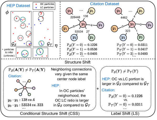
Figure 1: We illustrate structure shifts in real-world datasets: a) The HEP dataset in pileup mitigation tasks (Bertolini et al., 2014) has a shift in PU levels (change in the number of other collisions (OC) around the leading collision (LC) for proton-proton collision events), where $\mathcal{G}_{\mathcal{S}}$ is in PU30 and $\mathcal{G}_{\mathcal{T}}$ is in PU10; Here, in the green circles, the center nodes in grey are the particles whose labels are to be inferred. They have different ground-truth labels but the same neighborhood that includes one OC and one LC particle.b) The citation MAG dataset shifts in regions, where the source graph contains papers in the US and the target graph contains papers in German. More statistics on graph distribution shift from real-world examples can be found in Appendix E.5.

This work conducts a systematic study of the distinct challenges present in GDA and proposes a novel method, named Pairwise Alignment (Pair-Align) to tackle graph structure shift for node prediction tasks. Combined with feature alignment methods offered by traditional non-graph DA techniques (Ganin et al., 2016; Tachet des Combes et al., 2020), Pair-Align can in principle address a wide range of distribution shifts in graph data.

Our analysis begins with examining a graph with its adjacency matrix $\mathbf{A}$ and node labels $\mathbf{Y}$. We observe that graph structure shift ($\mathbb{P}_{\mathcal{S}}(\mathbf{A},\mathbf{Y})\neq\mathbb{P}_{\mathcal{T}}(\mathbf{A},\mathbf{Y})$) typically manifests as either conditional structure shift (CSS) or label shift (LS), or a combination of both. CSS refers to the change in neighboring connections among nodes within the same class ($\mathbb{P}_{\mathcal{S}}(\mathbf{A}|\mathbf{Y})\neq\mathbb{P}_{\mathcal{T}}(\mathbf{A}|\mathbf{Y})$) whereas LS denotes changes in the class distribution of nodes ($\mathbb{P}_{\mathcal{S}}(\mathbf{Y})\neq\mathbb{P}_{\mathcal{T}}(\mathbf{Y})$). These shifts are illustrated in Fig. 1 via examples in HEP and social networks, and are justified by statistics from several real-world applications.

In light of the two types of shifts, the Pair-Align method aims to estimate and subsequently mitigate the distribution shift in the neighboring nodes’ representations for any given node class $c$. To achieve this, Pair-Align employs a bootstrapping technique to recalibrate the influence of neighboring nodes in the message aggregation phase of GNNs. This strategic reweighting is key to effectively countering CSS. Concurrently, Pair-Align calculates label weights to alleviate disparities in the label distribution between source and target domains (addressing LS) by adjusting the classification loss. Pair-Align is depicted in Figure 2.

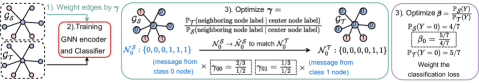
Figure 2: The pipeline contains modules in handling CSS with edge weights $\boldsymbol{\gamma}$ and handling LS with label weights $\boldsymbol{\beta}$

To demonstrate the effectiveness of our pipeline, we curate the regional MAG data that partitions large citation networks according to the regions where papers got published (Hu et al., 2020; Wang et al., 2020) to simulate the region shift. To the best of our knowledge, this is the largest dataset (of $\approx$ 380k nodes, 1.35M edges) to study GDA with data retrieved from the real-world database. We also include other graph data with shifts, like the pileup mitigation task studied in Liu et al. (2023). Our method shows strong performance in these two applications. Moreover, our method also outperforms baselines significantly in synthetic datasets and other real-world benchmark datasets.

2 Preliminaries and Related Works

2.1 Notation and The Problem Setup

We use capital letters, e.g., $Y$ to denote scalar random variables, and lower-case letters, e.g., $y$ to denote their realizations. The bold counterparts are used for their vector-valued correspondences, e.g., $\mathbf{Y},\mathbf{y}$, and the calligraphic letters, e.g. $\mathcal{Y}$, are for the value spaces. We always use capital letters to denote matrices. Let $\mathbb{P}$ denote a distribution, whose subscript $\mathcal{U}\in\{\mathcal{S},\mathcal{T}\}$ indicates the domain it depicts, e.g. $\mathbb{P}_{\mathcal{S}}(Y)$. The probability of a realization, e.g. $Y=y$, can then be denoted as $\mathbb{P}_{\mathcal{S}}(Y=y)$.

Graph Neural Networks (GNNs). We use $\mathcal{G}=(\mathcal{V},\mathcal{E},\mathbf{x})$ to denote a graph with the node set $\mathcal{V}$, the edge set $\mathcal{E}$ and node features $\mathbf{x}=[\cdots x_{u}\cdots]_{u\in\mathcal{V}}$. We focus on undirected graphs where the graph structure can also be represented as a symmetric adjacency matrix $\mathbf{A}$ where the entries $A_{uv}=A_{vu}=1$ when nodes $u,v$ form an edge and otherwise 0. GNNs take $\mathbf{A}$ and $\mathbf{x}$ as input and output node representations $\{h_{u},\forall u\in\mathcal{V}\}$. The standard GNNs (Hamilton et al., 2017) has a message-passing procedure. Specifically, with $h_{u}^{(1)}=x_{u}$, for each node $v$ and each layer $k\in[L]:=\{1,\ldots,L\}$,

$$h_{u}^{(k+1)}=\text{UPT}\,(h_{u}^{(k)},\text{AGG}\,(\{\mskip-5.0mu\{h_{v}^{(k)}:v\in\mathcal{N}_{u}\}\mskip-5.0mu\})),$$ (1)

where $\mathcal{N}_{v}$ denotes the set of neighbors of node $v$ and $\{\mskip-5.0mu\{\cdot\}\mskip-5.0mu\}$ denotes a multiset. The AGG function aggregates messages from the neighbors, and the UPT function updates the node representations. The last-layer node representation $h_{u}^{(L)}$ is used to predict the label $y_{u}\in\mathcal{Y}$ in node classification tasks.

Domain Adaptation (DA). In DA, each domain $\mathcal{U}\in\{S,T\}$ has its own joint feature and label distribution $\mathbb{P}_{\mathcal{U}}(X,Y)$. In the unsupervised setting, we have access to labeled source data $\{(x_{i},y_{i})\}_{i=1}^{N}$ and unlabeled target data $\{(x_{i})\}_{i=1}^{M}$ IID sampled from the source and target domain respectively. The model comprises a feature encoder $\phi:\mathcal{X}\rightarrow\mathcal{H}$ and a classifier $g:\mathcal{H}\rightarrow\mathcal{Y}$, with classification error in domain $\mathcal{U}$ denoted as $\varepsilon_{\mathcal{U}}(g\circ\phi)=\mathbb{P}_{\mathcal{U}}(g(\phi(X))\neq Y)$. The objective is to train the model with available data to minimize target error $\varepsilon_{\mathcal{T}}(g\circ\phi)$ when predicting target labels. A popular DA strategy is to learn domain-invariant representation, ensuring similar $\mathbb{P}_{\mathcal{S}}(H)$ and $\mathbb{P}_{\mathcal{T}}(H)$ and minimizing the source error $\varepsilon_{\mathcal{S}}(g\circ\phi)$ to retain classification capability simultaneously (Zhao et al., 2019). This is achieved through regularization of distance measures (Long et al., 2015; Zellinger et al., 2016) or adversarial training (Ganin et al., 2016; Tzeng et al., 2017; Zhao et al., 2018).

Graph Domain Adaptation (GDA). When extending unsupervised DA to the graph-structured data, we are given a source graph $\mathcal{G}_{\mathcal{S}}=(\mathcal{V}_{\mathcal{S}},\mathcal{E}_{\mathcal{S}},\mathbf{x}_{\mathcal{S}})$ with node labels $\mathbf{y}_{\mathcal{S}}$ and a target graph $\mathcal{G}_{\mathcal{T}}=(\mathcal{V}_{\mathcal{T}},\mathcal{E}_{\mathcal{T}},\mathbf{x}_{\mathcal{T}})$. The specific distribution and shifts in graph-structured data will be defined in Sec.3. The objective is similar to DA as to minimize the target error, but with the encoder $\phi$ switched to a GNN to predict node labels $\mathbf{y}_{\mathcal{T}}$ in the target graph.

2.2 Related Works and Existing Gaps

GDA research falls into two main categories, aiming at addressing domain adaptation for node and graph classification tasks respectively. Often, graph-level GDA problems can view each graph as an independent sample, allowing extension of previous non-graph DA techniques to graphs, such as causal inference (Rojas-Carulla et al., 2018; Peters et al., 2017) (more are reviewed in Appendix D). Conversely, node-level GDA presents challenges due to the interconnected nodes. Previous works mainly leveraged node representations as intermediaries to address these challenges.

The dominant idea of existing work on node-level GDA focused on aligning the marginal distributions of node representations, mostly over the last layer $\mathbf{h}^{(L)}$, across two graphs inspired by the domain invariant learning in DA (Liao et al., 2021). Some of them adopted adversarial training, such as (Dai et al., 2022; Zhang et al., 2019; Shen et al., 2020a). UDAGCN (Wu et al., 2020) calculated the point-wise mutual information and inter-graph attention to exploit local and global consistency on top of the adversarial training. Other works were motivated by regularizing different distance measures. Zhu et al. (2021) regularized over the central moment discrepancy (Zellinger et al., 2016). You et al. (2023) minimized the Wasserstein-1 distance between the distributions of node representations and controlled GNN Lipschitz via regularizing graph spectral properties. Wu et al. (2023) introduced graph subtree discrepancy inspired by the WL subtree kernel (Shervashidze et al., 2011) and suggested regularizing node representations after each layer of GNNs. Furthermore, Zhu et al. (2022, 2023) recognized that there could also be a shift in the label distribution, so they proposed to align the distribution of label/pseudo-label in addition to the marginal node representation.

Nonetheless, the marginal alignment methods above are inadequate when dealing with the structure shift consisting of CSS and LS. Firstly, these methods are flawed under LS. Based on $\mathbb{P}_{\mathcal{U}}(H^{(L)})=\sum_{Y}\mathbb{P}_{\mathcal{U}}(H^{(L)}|Y)\mathbb{P}_{\mathcal{U}}(Y)$, even if the marginal alignment $\mathbb{P}_{\mathcal{S}}(H^{(L)})=\mathbb{P}_{\mathcal{T}}(H^{(L)})$ is achieved, the conditional node representations will still mismatch $\mathbb{P}_{\mathcal{S}}(H^{(L)}|Y)\neq\mathbb{P}_{\mathcal{T}}(H^{(L)}|Y)$ under the LS, which induces more prediction error (Zhao et al., 2019; Tachet des Combes et al., 2020). Secondly, they are suboptimal under CSS. In particular, consider the HEP example in Fig. 1 (the particles in the two green circles) where CSS may yield the case that the label of the center particle (node) shifts, albeit with an unchanged neighborhood distribution. In this case, methods using a shared GNN encoder for marginal alignment definitely fail to make the correct prediction.

Liu et al. (2023) have recently analyzed this issue by using an example based on contextual stochastic block model (CSBM) (Deshpande et al., 2018) (defined in Appendix A).

Proposition 2.1.

(Liu et al., 2023) Suppose the source and target graphs are generated from the CSBM model of $n$ nodes with the same label distributions and node feature distributions. The edge connection probabilities are set to present a conditional structure shift $\mathbb{P}_{\mathcal{S}}(\mathbf{A}|\mathbf{Y})\neq\mathbb{P}_{\mathcal{T}}(\mathbf{A}|\mathbf{Y})$ and showcase the example that the ground truth label of the center node changes given the same neighborhood distribution. Then, by imposing $\mathbb{P}_{\mathcal{S}}(H^{(L)})=\mathbb{P}_{\mathcal{T}}(H^{(L)})$ through a GNN encoder $\phi$ shared across two domains, the target classification error with classifier g $\varepsilon_{\mathcal{T}}(g\circ\phi)\geq 0.25$, while if without such a constraint, there exists a GNN encoder $\phi$ such that $\varepsilon_{\mathcal{T}}(g\circ\phi)\rightarrow 0$ as $n\rightarrow\infty$.

To tackle this issue, Liu et al. (2023) proposed the StruRW method to reweight edges in the source graph based on weights derived from the CSBM model. However, StruRW still suffers from many issues. We will provide a more detailed comparison with StruRW in Sec. 3.5. To the best of our knowledge, our method is the first effort to address both CSS and LS in a principled way.

3 Pairwise Alignment for Structure Shift

We first define shifts in graphs as feature shift and structure shift, the latter includes both the Conditional Structure Shift (CSS) and the Label Shift (LS). Then, we analyze the objective of solving structure shift and propose our pairwise alignment algorithm that handles both CSS and LS.

3.1 Distribution Shifts in Graph-structured Data

Sec. 2.2 shows the sub-optimality of enforcing marginal node representation alignment under structure shifts. In fact, the necessity of conditional distribution alignment $\mathbb{P}_{\mathcal{S}}(H|Y)=\mathbb{P}_{\mathcal{T}}(H|Y)$ to deal with feature shift $\mathbb{P}_{\mathcal{S}}(X|Y)\neq\mathbb{P}_{\mathcal{T}}(X|Y)$ has been explored in non-graph scenarios, where $X$ denotes a feature vector and $H$ is the representation after $X$ passes through the encoder, i.e., $H=\phi(X)$. Early efforts such as Zhang et al. (2013); Gong et al. (2016) assumed that the shift in conditional representations from domain $\mathcal{S}$ to domain $\mathcal{T}$ follows a linear transformation and optimized conditional alignment by introducing an extra linear transformation to the source domain encoder to enhance conditional alignment $\mathbb{P}_{\mathcal{S}}(H|Y)=\mathbb{P}_{\mathcal{T}}(H|Y)$. Subsequent works learned the representations with adversarial training to enforce conditional alignment by aligning the joint distribution over the label predictions and representations (Long et al., 2018; Cicek & Soatto, 2019). Later, some works additionally considered label shift (Tachet des Combes et al., 2020; Liu et al., 2021) and proposed to match the label weighted $\mathbb{P}_{\mathcal{S}}^{\text{lw}}(H)$ with $\mathbb{P}_{\mathcal{T}}(H)$ with label weights estimated following Lipton et al. (2018).

In light of the limitations of existing works and the effort in non-graph DA research, it becomes clear that marginal alignment of node representations is insufficient for GDA, which underscores the importance of achieving conditional node representation alignment.

To address various distribution shifts for GDA in principle, we first decouple the potential distribution shifts in graph data by defining feature shift and structure shift in terms of conditional distributions and label distributions. Our data generation process can be characterized by the following model: $\mathbf{X}\leftarrow\mathbf{Y}\rightarrow\mathbf{A}$, where labels are drawn at each node first, and then edges as well as features at each node are generated. Under this model, we define the following feature shift, which denotes the change of the conditional feature generation process given the labels.

Definition 3.1 (Feature Shift).

Assume the node features $x_{u}$, $u\in\mathcal{V}$ are IID sampled from $\mathbb{P}(X|Y)$ given node labels $y_{u}$. Therefore, the conditional distribution of $\mathbf{x}|\mathbf{y}$, $\mathbb{P}(\mathbf{X}=\mathbf{x}|\mathbf{Y}=\mathbf{y})=\prod_{u\in\mathcal{V}}\mathbb{P}(X=x_{u}|Y=y_{u})$. The feature shift is then defined as $\mathbb{P}_{\mathcal{S}}(X|Y)\neq\mathbb{P}_{\mathcal{T}}(X|Y)$.

Definition 3.2 (Structure Shift).

Given the joint distribution of the adjacency matrix and node labels $\mathbb{P}(\mathbf{A},\mathbf{Y})$. The Structure Shift is defined as $\mathbb{P}_{\mathcal{S}}(\mathbf{A},\mathbf{Y})\neq\mathbb{P}_{\mathcal{T}}(\mathbf{A},\mathbf{Y})$. With decomposition as $\mathbb{P}_{\mathcal{U}}(\mathbf{A},\mathbf{Y})=\mathbb{P}_{\mathcal{U}}(\mathbf{A}|\mathbf{Y})\mathbb{P}_{\mathcal{U}}(\mathbf{Y})$, it results in Conditional Structure Shift (CSS) and Label Shift (LS):

• CSS: $\mathbb{P}_{\mathcal{S}}(\mathbf{A}|\mathbf{Y})\neq\mathbb{P}_{\mathcal{T}}(\mathbf{A}|\mathbf{Y})$

• LS: $\mathbb{P}_{\mathcal{S}}(\mathbf{Y})\neq\mathbb{P}_{\mathcal{T}}(\mathbf{Y})$

As shown in Fig. 1, structure shift consisting of CSS and LS widely exists in real-world applications. Feature shift here, which is equivalent to the conditional feature shift in non-graph literature, can be addressed by adapting conventional conditional shift methods. So, later, we assume that feature shift has been addressed, i.e., $\mathbb{P}_{\mathcal{S}}(X|Y)=\mathbb{P}_{\mathcal{T}}(X|Y)$.

In contrast, structure shift is unique to graph data due to the non-IID nature caused by node interconnections. Moreover, the learning of node representations is intrinsically linked to the graph structure as the GNN encoder takes $\mathbf{A}$ as input. Therefore, even if after one layer of GNN, $\mathbb{P}_{\mathcal{S}}(H^{(k)}|Y)=\mathbb{P}_{\mathcal{T}}(H^{(k)}|Y)$ is achieved, CSS could still lead to misalignment of conditional node representation distributions in the next layer $\mathbb{P}_{\mathcal{S}}(H^{(k+1)}|Y)\neq\mathbb{P}_{\mathcal{T}}(H^{(k+1)}|Y)$. Accordingly, a tailored algorithm is needed to remove this effect of CSS, which, when combined with techniques for LS, can effectively resolve the structure shift.

3.2 Addressing Conditional Structure Shift

To remove the effect of CSS under GNN, the objective is to guarantee $\mathbb{P}_{\mathcal{S}}(H^{(k+1)}|Y)=\mathbb{P}_{\mathcal{T}}(H^{(k+1)}|Y)$ given $\mathbb{P}_{\mathcal{S}}(H^{(k)}|Y)=\mathbb{P}_{\mathcal{T}}(H^{(k)}|Y)$. Considering one layer of GNN encoding in Eq. (1): given $\mathbb{P}_{\mathcal{S}}(H^{(k)}|Y)=\mathbb{P}_{\mathcal{T}}(H^{(k)}|Y)$ , the mismatch in $k+1$ layer may arise from the distribution shift of the neighboring multiset $\{\mskip-5.0mu\{h_{v}^{(k)}:v\in\mathcal{N}_{u}\}\mskip-5.0mu\}$ given the center node label $y_{u}$. Therefore, the key is to transform the neighboring multisets in the source graph to achieve conditional alignment with the target domain regarding the distributions of such neighboring multisets. Our approach first starts with a sufficient condition for such conditional alignment.

Theorem 3.3 (Sufficient conditions for addressing CSS).

Given the following assumptions

• (Conditional Alignment in the previous layer $k$) $\mathbb{P}_{\mathcal{S}}(H^{(k)}|Y)=\mathbb{P}_{\mathcal{T}}(H^{(k)}|Y)$ and $\forall u\in\mathcal{V}_{\mathcal{U}}$, given $Y=y_{u}$, $h_{u}^{(k)}$ is independently sampled from $\mathbb{P}_{\mathcal{U}}(H^{(k)}|Y)$.

• (Edge Conditional Independence) Given node labels $\mathbf{y}$, edges mutually independently exist in the graph.

if there exists a transformation that modifies the neighborhood of node $u$: $\mathcal{N}_{u}\rightarrow\tilde{\mathcal{N}}_{u},\forall u\in\mathcal{V}_{\mathcal{S}}$, such that $\mathbb{P}_{\mathcal{S}}(|\tilde{\mathcal{N}}_{u}||Y_{u}=i)=\mathbb{P}_{\mathcal{T}}(|\mathcal{N}_{u}||Y_{u}=i)$ and $\mathbb{P}_{\mathcal{S}}(Y_{v}|Y_{u}=i,v\in\tilde{\mathcal{N}}_{u})=\mathbb{P}_{\mathcal{T}}(Y_{v}|Y_{u}=i,v\in\mathcal{N}_{u})$, $\forall i\in\mathcal{Y}$, then $\mathbb{P}_{\mathcal{S}}(H^{(k+1)}|Y)=\mathbb{P}_{\mathcal{T}}(H^{(k+1)}|Y)$ is satisfied.

Remark 3.4.

The assumption edge conditional independence essentially assumes an SBM model for the graph structure, which is widely adopted for graph learning algorithm analysis (Liu et al., 2023; Wei et al., 2022).

This theorem reveals that it suffices to align two distributions with the multiset transformation on the source graph: 1) the distribution of the degree/cardinality of the neighbors $\mathbb{P}_{\mathcal{U}}(|\mathcal{N}_{u}||Y_{u})$ and 2) the node label distribution in the neighborhood $\mathbb{P}_{\mathcal{U}}(Y_{v}|Y_{u},v\in\mathcal{N}_{u})$, both conditioned on the center node label $Y_{u}$.

Multiset Alignment. Bootstrapping the elements in the multisets can be used to align the two distributions. In the context of GNNs, which typically employ sum/mean pooling functions to aggregate the multisets, such a bootstrapping process can be translated into assigning weights to different neighboring nodes given their labels and the center node’s label. Moreover, practically, mean pooling is often the preferred choice due to its superior empirical performance, which is also observed in our experiments. Aligning the distributions of the node degrees $\mathbb{P}_{\mathcal{U}}(|\mathcal{N}_{u}||Y_{u})$ yields negligible impact with mean pooling (Xu et al., 2018). Therefore, our method focuses on aligning the distribution $\mathbb{P}_{\mathcal{U}}(Y_{v}|Y_{u},v\in\mathcal{N}_{u})$, in which the edge weights are the ratios of such probabilities across two domains:

Definition 3.5.

Assume $\mathbb{P}_{\mathcal{S}}(Y_{v}=j|Y_{u}=i,v\in\mathcal{N}_{u})>0,\forall i,j\in\mathcal{Y}$, we define $\boldsymbol{\gamma}\in\mathbb{R}^{|\mathcal{Y}|\times|\mathcal{Y}|}$ as:

$$[\boldsymbol{\gamma}]_{i,j}=\frac{\mathbb{P}_{\mathcal{T}}(Y_{v}=j|Y_{u}=i,v\in\mathcal{N}_{u})}{\mathbb{P}_{\mathcal{S}}(Y_{v}=j|Y_{u}=i,v\in\mathcal{N}_{u})},\forall i,j\in\mathcal{Y}$$

where $[\boldsymbol{\gamma}]_{i,j}$ is the density ratio between the target and source graphs from class-$i$ nodes to class-$j$ nodes. Note that $[\boldsymbol{\gamma}]_{i,j}\neq[\boldsymbol{\gamma}]_{j,i}$. To differentiate the encoding with and without the adjusted edge weights for the source and target graphs, we denote the operation that first adjusts the edge weights $\boldsymbol{\gamma}$ and then apply GNN encoding as $\phi_{\boldsymbol{\gamma}}$ while the one that directly applies GNN encoding as $\phi$. By assuming the conditions made in Thm 3.3 and applying them in an iterative manner for each layer of GNN, the last-layer alignment $\mathbb{P}_{\mathcal{S}}(H^{(L)}|Y)=\mathbb{P}_{\mathcal{T}}(H^{(L)}|Y)$ can be achieved with $\mathbf{h}^{(L)}_{\mathcal{S}}=\phi_{\gamma}(\mathbf{x}_{\mathcal{S}},\mathbf{A}_{\mathcal{S}})$ and $\mathbf{h}^{(L)}_{\mathcal{T}}=\phi(\mathbf{x}_{\mathcal{T}},\mathbf{A}_{\mathcal{T}})$. Note that based on conditional alignment in the distribution of randomly sampled node representations $\mathbb{P}_{\mathcal{S}}(H^{(L)}|Y)=\mathbb{P}_{\mathcal{T}}(H^{(L)}|Y)$ and under the conditions in Thm 3.3, $\mathbb{P}_{\mathcal{S}}(\mathbf{H}^{(L)}|\mathbf{Y})=\mathbb{P}_{\mathcal{T}}(\mathbf{H}^{(L)}|\mathbf{Y})$ can also be achieved in the matrix form.

$\boldsymbol{\gamma}$ Estimation. Till now we explain why edge reweighting using $\boldsymbol{\gamma}$ can address CSS for GNN encoding, we will detail our pairwise alignment method to obtain $\boldsymbol{\gamma}$ next. By definition, $\boldsymbol{\gamma}$ can be decomposed into another two weights.

Definition 3.6.

Assume $\mathbb{P}_{\mathcal{S}}(Y_{u}=i,Y_{v}=j|e_{uv}\in\mathcal{E}_{\mathcal{S}})>0,\forall i,j\in\mathcal{Y}$, we define $\mathbf{w}\in\mathbb{R}^{|\mathcal{Y}|\times|\mathcal{Y}|}$ and $\boldsymbol{\alpha}\in\mathbb{R}^{|\mathcal{Y}|\times 1}$ as:

$$[\mathbf{w}]_{i,j} =\frac{\mathbb{P}_{\mathcal{T}}(Y_{u}=i,Y_{v}=j|e_{uv}\in\mathcal{E}_{\mathcal{T}})}{\mathbb{P}_{\mathcal{S}}(Y_{u}=i,Y_{v}=j|e_{uv}\in\mathcal{E}_{\mathcal{S}})},$$

$$[\boldsymbol{\alpha}]_{i} =\frac{\mathbb{P}_{\mathcal{T}}(Y_{u}=i|e_{uv}\in\mathcal{E}_{\mathcal{T}})}{\mathbb{P}_{\mathcal{S}}(Y_{u}=i|e_{uv}\in\mathcal{E}_{\mathcal{S}})},\forall i,j\in\mathcal{Y}$$

and $\boldsymbol{\gamma}$ can be estimated via

$$\boldsymbol{\gamma}=\text{diag}(\boldsymbol{\alpha})^{-1}\mathbf{w}$$ (2)

For domain $\mathcal{U}$, $\mathbb{P}_{\mathcal{U}}(Y_{u},Y_{v}|e_{uv}\in\mathcal{E}_{\mathcal{U}})$ is the joint distribution of the label pairs of two nodes that form an edge, which can be computed for domain $\mathcal{S}$ but not for domain $\mathcal{T}$. $\mathbb{P}_{\mathcal{U}}(Y_{u}|e_{uv}\in\mathcal{E}_{\mathcal{U}})$ can be obtained by marginalizing $\mathbb{P}_{\mathcal{U}}(Y_{u},Y_{v}|e_{uv}\in\mathcal{E}_{\mathcal{U}})$ over $Y_{v}$, as $\mathbb{P}_{\mathcal{U}}(Y_{u}=i|e_{uv}\in\mathcal{E}_{\mathcal{U}})=\sum_{j\in\mathcal{Y}}\mathbb{P}_{\mathcal{U}}(Y_{u}=i,Y_{v}=j|e_{uv}\in\mathcal{E}_{\mathcal{U}})$. Also, it is crucial to differentiate $\mathbb{P}_{\mathcal{U}}(Y_{u}|e_{uv}\in\mathcal{E}_{\mathcal{U}})$ from $\mathbb{P}_{\mathcal{U}}(Y)$: the former is the label distribution of the end node conditioned on an edge, while the latter is the label distribution of nodes without conditions. Given $\mathbf{w}$ and two distributions computed over the source graph, $\boldsymbol{\alpha}$ can be derived via

$$[\boldsymbol{\alpha}]_{i}=\frac{\sum_{j\in\mathcal{Y}}([\mathbf{w}]_{i,j}\mathbb{P}_{\mathcal{S}}(Y_{u}=i,Y_{v}=j|e_{uv}\in\mathcal{E}_{\mathcal{S}}))}{\mathbb{P}_{\mathcal{S}}(Y_{u}=i|e_{uv}\in\mathcal{E}_{\mathcal{S}})},$$ (3)

so next, we proceed to estimate $\mathbf{w}$ to complete $\boldsymbol{\gamma}$ calculation.

Pair-wise Alignment. Note that if $(Y_{u},Y_{v})$ is viewed as a type for edge $e_{uv}$, $\mathbb{P}_{\mathcal{U}}(Y_{u},Y_{v}|e_{uv}\in\mathcal{E}_{\mathcal{U}})$ essentially represents an edge-type distribution. In practice, we use pair-wise pseudo-label distribution alignment to estimate $\mathbf{w}$.

Definition 3.7.

Let $\boldsymbol{\Sigma}\in\mathbb{R}^{|\mathcal{Y}|^{2}\times|\mathcal{Y}|^{2}}$ denote the matrix that stands for the joint distribution of the predicted types of edges and the true types of edges, and $\boldsymbol{\nu}\in\mathbb{R}^{|\mathcal{Y}|^{2}\times 1}$ denote the distribution of the predicted types of edges for the target domain, $\forall i,j,i^{\prime},j^{\prime}\in\mathcal{Y}$

$$[\boldsymbol{\Sigma}]_{ij,i^{\prime}j^{\prime}} =\mathbb{P}_{\mathcal{S}}(\hat{Y}_{u}=i,\hat{Y}_{v}=j,Y_{u}=i^{\prime},Y_{v}=j^{\prime}|e_{uv}\in\mathcal{E}_{\mathcal{S}})$$

$$[\boldsymbol{\nu}]_{ij} =\mathbb{P}_{\mathcal{T}}(\hat{Y}_{u}=i,\hat{Y}_{v}=j|e_{uv}\in\mathcal{E}_{\mathcal{T}})$$

Specifically, similar to Tachet des Combes et al. (2020, Lemma 3.2), Lemma 3.8 shows that $\mathbf{w}$ can be obtained by solving the linear system $\boldsymbol{\nu}=\boldsymbol{\Sigma}\mathbf{w}$ if $\mathbb{P}_{\mathcal{S}}(H^{(L)}|Y)=\mathbb{P}_{\mathcal{T}}(H^{(L)}|Y)$ is satisfied.

Lemma 3.8.

If $\mathbb{P}_{\mathcal{S}}(H^{(L)}|Y)=\mathbb{P}_{\mathcal{T}}(H^{(L)}|Y)$ is satisfied, and node representations are conditionally independent of graph structures given node labels, then $\boldsymbol{\nu}=\boldsymbol{\Sigma}\mathbf{w}$.

Empirically, we estimate $\hat{\boldsymbol{\Sigma}}$ and $\hat{\boldsymbol{\nu}}$ based on the classifier $g$, where $g(h_{u}^{(L)})$ denotes the soft label of node $u$. Specifically, $[\hat{\boldsymbol{\Sigma}}]_{ij,i^{\prime}j^{\prime}}=\frac{1}{|\mathcal{E}_{\mathcal{S}}|}\sum_{e_{uv}\in\mathcal{E}_{\mathcal{S}},y_{u}=i^{\prime},y_{v}=j^{\prime}}[g(h_{u}^{(L)})]_{i}\times[g(h_{v}^{(L)})]_{j}$, and $[\hat{\boldsymbol{\nu}}]_{ij}=\frac{1}{|\mathcal{E}_{\mathcal{T}}|}\sum_{e_{u^{\prime}v^{\prime}}\in\mathcal{E}_{\mathcal{T}}}[g(h_{u^{\prime}}^{(L)})]_{i}\times[g(h_{v^{\prime}}^{(L)})]_{j}$. Then, $\mathbf{w}$ can be solved via:

$$\min_{\mathbf{w}}\quad\lVert\hat{\boldsymbol{\Sigma}}\mathbf{w}-\hat{\boldsymbol{\nu}}\rVert_{2},\quad\text{s.t.}\;\mathbf{w}\geq 0,\,\text{and}$$ (4)

$$\,\sum_{i,j}[\mathbf{w}]_{i,j}\mathbb{P}_{\mathcal{S}}(Y_{u}=i,Y_{v}=j|e_{uv}\in\mathcal{E}_{\mathcal{S}})=1,$$

where the constraints guarantee a valid target edge type distribution $\mathbb{P}_{\mathcal{T}}(Y_{u},Y_{v}|e_{uv}\in\mathcal{E}_{\mathcal{T}})$. For undirected graphs, $\mathbf{w}$ can be symmetric, so we may add an extra constraint $[\mathbf{w}]_{i,j}=[\mathbf{w}]_{j,i}$. Finally, we calculate $\boldsymbol{\alpha}$ following Eq. (3) with the obtained $\mathbf{w}$ and compute $\boldsymbol{\gamma}$ via Eq. (2). Note that in Appendix C.1, we will discuss how to improve the robustness of the estimations of $\mathbf{w}$ and $\boldsymbol{\gamma}$.

In summary, handling CSS is an iterative process where we begin by employing an estimated $\boldsymbol{\gamma}$ as edge weights on the source graph to reduce the gap between $\mathbb{P}_{\mathcal{S}}(H^{(L)}|Y)$ and $\mathbb{P}_{\mathcal{T}}(H^{(L)}|Y)$ due to Thm 3.3. With a reduced gap, we can estimate $\mathbf{w}$ more accurately (due to Lemma 3.8) and thus improve the estimation of $\boldsymbol{\gamma}$. Through iterative refinement, $\boldsymbol{\gamma}$ progressively enhances the conditional alignment $\mathbb{P}_{\mathcal{S}}(H^{(L)}|Y)=\mathbb{P}_{\mathcal{T}}(H^{(L)}|Y)$ to address CSS.

3.3 Addressing Label Shift

Inspired by the techniques in Lipton et al. (2018); Azizzadenesheli et al. (2018), we estimate the ratio between the source and target label distribution by aligning the node-level pseudo-label distribution to address LS.

Definition 3.9.

Assume $\mathbb{P}_{\mathcal{S}}(Y_{u}=i)>0,\forall i\in\mathcal{Y}$, we define $\boldsymbol{\beta}\in\mathbb{R}^{|\mathcal{Y}|\times 1}$ as the weights of the source and target label distribution: $[\boldsymbol{\beta}]_{i}=\frac{\mathbb{P}_{\mathcal{T}}(Y=i)}{\mathbb{P}_{\mathcal{S}}(Y=i)},\forall i\in\mathcal{Y}$.

Definition 3.10.

Let $\mathbf{C}\in\mathbb{R}^{|\mathcal{Y}|\times|\mathcal{Y}|}$ denote the confusion matrix of the classifier for the source domain, and $\boldsymbol{\mu}\in\mathbb{R}^{|\mathcal{Y}|\times 1}$ denote the distribution of the label predictions for the target domain, $\forall i,i^{\prime}\in\mathcal{Y}$

$$[\mathbf{C}]_{i,i^{\prime}}=\mathbb{P}_{\mathcal{S}}(\hat{Y}=i,Y=i^{\prime}),\quad[\boldsymbol{\mu}]_{i}=\mathbb{P}_{\mathcal{T}}(\hat{Y}=i)$$

The key insight is similar to the estimation of $\mathbf{w}$, when $\mathbb{P}_{\mathcal{S}}(H^{(L)}|Y)=\mathbb{P}_{\mathcal{T}}(H^{(L)}|Y)$ is satisfied, $\boldsymbol{\beta}$ can be estimated by solving a linear system $\boldsymbol{\mu}=\mathbf{C}\boldsymbol{\beta}$,

Lemma 3.11.

If $\mathbb{P}_{\mathcal{S}}(H^{(L)}|Y)=\mathbb{P}_{\mathcal{T}}(H^{(L)}|Y)$ is satisfied, and node representations are conditionally independent of each other given the node labels, then $\boldsymbol{\mu}=\mathbf{C}\boldsymbol{\beta}$.

Empirically, with $\hat{\mathbf{C}}$ and $\hat{\boldsymbol{\mu}}$ can be estimated as $[\hat{\mathbf{C}}]_{i,i^{\prime}}=\frac{1}{|\mathcal{V}_{\mathcal{S}}|}\sum_{u\in\mathcal{V}_{\mathcal{S}},y_{u}=i^{\prime}}[g(h_{u}^{(L)})]_{i}$ and $[\hat{\boldsymbol{\mu}}]_{i}=\frac{1}{|\mathcal{V}_{\mathcal{T}}|}\sum_{u^{\prime}\in\mathcal{V}_{\mathcal{T}}}[g(h_{u^{\prime}}^{(L)})]_{i}$. $\boldsymbol{\beta}$ can be solved with a least square problem with the constraints to guarantee a valid target label distribution $\mathbb{P}_{\mathcal{T}}(Y)$.

$$\min_{\boldsymbol{\beta}}\lVert\hat{\mathbf{C}}\boldsymbol{\beta}-\hat{\boldsymbol{\mu}}\rVert_{2},\,\text{s.t.}\;\boldsymbol{\beta}\geq 0,\,\sum_{i}[\boldsymbol{\beta}]_{i}\mathbb{P}_{\mathcal{S}}(Y=i)=1$$ (5)

We use $\boldsymbol{\beta}$ to weight the classification loss to handle LS. Combined with the previous module that uses $\boldsymbol{\gamma}$ to solve for CSS, our algorithm completely addresses the structure shift.

3.4 Algorithm Overview

Now, we are able to put everything together. The entire algorithm is shown in Alg. 1. At the start of each epoch, the estimated $\boldsymbol{\gamma}$ are used as edge weights in the source graph (line 4). Then, GNN $\phi_{\boldsymbol{\gamma}}$ paired with $\boldsymbol{\gamma}$ yields node representations that further pass through the classifier $g$ to get soft labels $\hat{\mathbf{Y}}$ (line 5). The model is trained via the loss $\mathcal{L}_{C}^{\boldsymbol{\beta}}$, i.e., a $\boldsymbol{\beta}$-weighted cross-entropy loss (line 6):

$$\mathcal{L}_{C}^{\boldsymbol{\beta}}=\frac{1}{|\mathcal{V}_{\mathcal{S}}|}\sum_{v\in\mathcal{V}_{\mathcal{S}}}[\boldsymbol{\beta}]_{y_{v}}\text{cross-entropy}(y_{v},\hat{y}_{v})$$ (6)

Then, with every $t$ epoch, update the estimations of $\mathbf{w}$, $\boldsymbol{\gamma}$, and $\boldsymbol{\beta}$ for the next epoch (lines 7-10).

Algorithm 1 Pairwise Alignment

1:  Input The source graph $\mathcal{G}_{\mathcal{S}}$ with node labels $\mathbf{Y}_{\mathcal{S}}$; The target graph $\mathcal{G}_{\mathcal{T}}$; A GNN $\phi$ and a classifier $g$; The total epoch number $n$, the epoch period $t$ for weight update.

2:  Initialize $\mathbf{w},\boldsymbol{\gamma},\boldsymbol{\beta}=\mathbf{1},$

3:  while epoch $<n$ or  not converged do

4:     Add edge weights to $\mathcal{G}_{\mathcal{S}}$ according to $\boldsymbol{\gamma}$

5:     Get $\hat{\mathbf{Y}}_{\mathcal{S}}=g(\phi_{\boldsymbol{\gamma}}(\mathbf{x}_{\mathcal{S}},\mathbf{A}_{\mathcal{S}}))$ in the source domain

6:     Update $\phi$ and $g$ as $\min_{\phi,g}\mathcal{L}_{C}^{\boldsymbol{\beta}}(\hat{\mathbf{Y}}_{\mathcal{S}},\mathbf{Y}_{\mathcal{S}})$ Eq. (6)

7:     if $\text{epoch}\equiv 0\,(\text{mod}\,t)$ then

8:        Get $\hat{\mathbf{Y}}_{\mathcal{S}}$ and $\hat{\mathbf{Y}}_{\mathcal{T}}=g(\phi(\mathbf{x}_{\mathcal{T}},\mathbf{A}_{\mathcal{T}}))$

9:        Update the estimation of $\hat{\boldsymbol{\Sigma}},\hat{\boldsymbol{\nu}}$, $\hat{\mathbf{C}},\hat{\boldsymbol{\mu}}$

10:        Optimize for $\mathbf{w}$ Eq.(4) and calculate for $\boldsymbol{\gamma}$ Eq.(2)

11:        Optimize for $\boldsymbol{\beta}$ following Eq.(5)

12:     end if

13:  end while

3.5 Comparison to StruRW (Liu et al., 2023)

The edge weights estimation in StruRW and Pair-Align differ in two major points. First, StruRW computes edge weights as the ratio of the source and target edge connection probabilities. This by definition, if using our notations, corresponds to $\mathbf{w}$ instead of $\boldsymbol{\gamma}$ and ignores the effect of $\boldsymbol{\alpha}$. However, Thm 3.3 shows that using $\boldsymbol{\gamma}$ is the key to reduce CSS. Second, even for the estimation of $\mathbf{w}$, StruRW suffers from inaccurate estimation. In our notation, StruRW simply assumes that $\mathbb{P}_{\mathcal{S}}(\hat{Y}=i|Y=i)=1,\forall i\in\mathcal{Y}$, i.e., perfect training in the source domain and uses hard pseudo-labels in the target domain to estimate $\mathbf{w}$. In contrast, our optimization to obtain $\mathbf{w}$ is more stable. Moreover, StruRW ignores the effect of LS entirely. From this perspective, StruRW can be understood as a special case of Pair-Align under the assumption of no LS and perfect prediction in the target graph. Furthermore, our work is the first to rigorously formulate the idea of conditional alignment in graphs.

4 Experiments

Table 1: Performance on MAG datasets (accuracy scores). The bold font and underline indicate the best model and baseline respectively

Domains $US\rightarrow CN$ $US\rightarrow DE$ $US\rightarrow JP$ $US\rightarrow RU$ $US\rightarrow FR$ $CN\rightarrow US$ $CN\rightarrow DE$ $CN\rightarrow JP$ $CN\rightarrow RU$ $CN\rightarrow FR$ ERM $26.92\pm 1.08$ $26.37\pm 1.16$ $37.63\pm 0.36$ $21.71\pm 0.38$ $20.11\pm 0.34$ $31.47\pm 1.25$ $13.29\pm 0.36$ $22.15\pm 0.89$ $10.92\pm 0.82$ $10.86\pm 1.04$ DANN $24.20\pm 1.19$ $26.29\pm 1.44$ $\underline{37.92}\pm 0.25$ $21.76\pm 1.58$ $20.71\pm 0.29$ $30.23\pm 0.99$ $13.46\pm 0.40$ $21.48\pm 1.26$ $11.94\pm 1.90$ $10.65\pm 0.53$ IWDAN $23.39\pm 0.93$ $25.97\pm 0.41$ $34.98\pm 0.68$ $22.80\pm 3.03$ $21.75\pm 0.81$ $31.72\pm 1.24$ $13.39\pm 1.06$ $19.86\pm 1.21$ $10.93\pm 1.33$ $11.64\pm 4.56$ UDAGCN OOM OOM OOM OOM OOM OOM OOM OOM OOM OOM StruRW $\underline{31.58}\pm 3.10$ $\underline{30.03}\pm 2.23$ $37.20\pm 0.27$ $\underline{28.97}\pm 2.98$ $\underline{22.73}\pm 1.73$ $\underline{37.08}\pm 1.09$ $\underline{19.93}\pm 1.82$ $\underline{29.76}\pm 2.56$ $\underline{17.94}\pm 9.82$ $\underline{15.81}\pm 3.76$ SpecReg $23.74\pm 1.32$ $26.68\pm 1.44$ $37.68\pm 0.25$ $21.47\pm 0.84$ $20.91\pm 0.53$ $26.52\pm 1.75$ $13.76\pm 0.65$ $20.50\pm 0.08$ $10.50\pm 0.53$ $10.45\pm 1.16$ PA-CSS $37.93\pm 1.65$ $38.49\pm 2.66$ $47.38\pm 0.61$ $35.07\pm 10.2$ $\mathbf{28.64}\pm 0.08$ $43.28\pm 0.16$ $25.91\pm 2.70$ $37.42\pm 5.64$ $32.05\pm 0.81$ $22.83\pm 2.46$ PA-LS $27.00\pm 0.50$ $26.89\pm 0.90$ $38.96\pm 0.94$ $21.42\pm 0.91$ $20.63\pm 0.45$ $31.21\pm 1.45$ $15.02\pm 1.04$ $23.22\pm 0.57$ $11.44\pm 0.57$ $11.16\pm 0.56$ PA-BOTH $\mathbf{40.06}\pm 0.99$ $\mathbf{38.85}\pm 4.71$ $\mathbf{47.43}\pm 1.82$ $\mathbf{37.07}\pm 5.28$ $25.21\pm 3.79$ $\mathbf{45.16}\pm 0.50$ $\mathbf{26.19}\pm 1.01$ $\mathbf{38.26}\pm 2.27$ $\mathbf{33.34}\pm 1.94$ $\mathbf{24.16}\pm 1.13$

Table 2: Performance on Pileup datasets (f1 scores). The bold font and underline indicate the best model and baseline respectively

Pileup Conditions Physical Processes Domains $\text{PU}10\rightarrow 30$ $\text{PU}30\rightarrow 10$ PU$10\rightarrow 50$ PU$50\rightarrow 10$ PU$30\rightarrow 140$ PU$140\rightarrow 30$ $gg\rightarrow qq$ $qq\rightarrow gg$ ERM $48.17\pm 3.87$ $64.17\pm 1.50$ $48.73\pm 0.45$ $70.11\pm 1.12$ $18.76\pm 1.50$ $33.02\pm 28.77$ $\underline{67.70}\pm 0.31$ $72.63\pm 0.54$ DANN $49.99\pm 2.07$ $64.62\pm 0.70$ $48.44\pm 0.78$ $68.70\pm 1.42$ $28.20\pm 1.20$ $21.95\pm 20.37$ $66.48\pm 0.67$ $71.78\pm 0.87$ IWDAN $35.85\pm 1.73$ $62.24\pm 0.15$ $26.49\pm 0.40$ $67.82\pm 0.62$ $8.91\pm 3.17$ $\underline{40.02}\pm 1.93$ $66.85\pm 0.69$ $\underline{73.10}\pm 0.29$ UDAGCN $45.39\pm 2.07$ $62.27\pm 1.23$ $44.75\pm 1.76$ $68.93\pm 0.55$ $19.95\pm 0.84$ $29.66\pm 5.57$ $65.99\pm 1.06$ $71.99\pm 0.61$ StruRW $52.41\pm 1.74$ $\underline{67.72}\pm 0.22$ $47.25\pm 1.96$ $\underline{70.93}\pm 0.66$ $\underline{37.81}\pm 0.64$ $37.84\pm 2.82$ $67.66\pm 0.55$ $72.72\pm 0.68$ SpecReg $\underline{52.61}\pm 1.06$ $65.34\pm 0.62$ $\underline{48.85}\pm 0.94$ $67.95\pm 2.23$ $28.86\pm 1.58$ $28.79\pm 25.83$ $66.66\pm 0.40$ $72.73\pm 0.42$ PA-CSS $\mathbf{56.00}\pm 0.14$ $58.44\pm 3.19$ $50.77\pm 0.70$ $60.95\pm 6.09$ $40.31\pm 0.31$ $37.24\pm 7.69$ $67.75\pm 0.27$ $73.24\pm 0.38$ PA-LS $46.84\pm 0.45$ $67.12\pm 0.65$ $48.51\pm 1.46$ $71.17\pm 0.70$ $36.29\pm 0.92$ $46.38\pm 0.96$ $67.63\pm 0.38$ $\mathbf{73.40}\pm 0.13$ PA-BOTH $55.45\pm 0.21$ $\mathbf{68.29}\pm 0.41$ $\mathbf{51.43}\pm 0.42$ $\mathbf{71.23}\pm 0.63$ $\mathbf{40.53}\pm 0.25$ $\mathbf{51.21}\pm 2.88$ $\mathbf{67.77}\pm 0.70$ $73.36\pm 0.12$

Table 3: Synthetic CSBM results (accuracy). The bold font and the underline indicate the best model and baseline respectively

CSS (only class ratio shift) CSS (only degree shift) CSS (shift in both) CSS + LS ERM $94.22\pm 0.97$ $57.04\pm 3.83$ $99.01\pm 0.28$ $96.21\pm 0.27$ $88.90\pm 0.22$ $58.01\pm 1.91$ $61.35\pm 4.64$ $61.65\pm 0.80$ IWDAN $95.85\pm 0.70$ $76.75\pm 1.32$ $98.97\pm 0.05$ $\textbf{97.15}\pm 0.33$ $\underline{93.65}\pm 0.70$ $79.53\pm 3.57$ $\underline{92.42}\pm 0.72$ $\underline{87.01}\pm 2.14$ UDAGCN $96.82\pm 0.70$ $69.93\pm 5.17$ $\textbf{99.52}\pm 0.05$ $\underline{97.04}\pm 0.28$ $93.17\pm 1.02$ $67.44\pm 4.95$ $87.67\pm 3.21$ $83.69\pm 2.35$ StruRW $\underline{96.83}\pm 0.33$ $\underline{86.65}\pm 5.62$ $98.87\pm 0.19$ $95.93\pm 0.55$ $92.09\pm 0.55$ $\underline{80.00}\pm 7.49$ $75.38\pm 12.11$ $75.96\pm 2.96$ SpecReg $93.46\pm 1.21$ $62.97\pm 1.01$ $98.94\pm 0.03$ $96.69\pm 0.23$ $89.58\pm 1.58$ $61.28\pm 1.19$ $76.73\pm 3.18$ $83.40\pm 1.38$ PA-CSS $96.65\pm 1.21$ $91.79\pm 1.68$ $98.92\pm 0.52$ $96.24\pm 0.23$ $94.99\pm 0.49$ $91.20\pm 0.95$ $94.95\pm 0.69$ $\mathbf{95.66}\pm 0.45$ PA-LS $94.22\pm 0.95$ $57.14\pm 3.73$ $\underline{99.02}\pm 0.29$ $96.17\pm 0.26$ $88.85\pm 0.22$ $57.96\pm 1.84$ $61.39\pm 4.59$ $67.91\pm 9.98$ PA-BOTH $\mathbf{97.24}\pm 0.33$ $\mathbf{91.97}\pm 1.49$ $98.20\pm 1.04$ $96.25\pm 0.33$ $\mathbf{95.44}\pm 0.51$ $\mathbf{91.67}\pm 0.38$ $\mathbf{95.24}\pm 0.11$ $95.55\pm 0.65$

Table 4: Performance on Arxiv and DBLP/ACM datasets (accuracy). The bold and underline indicate the best model and baseline

1950-2007 1950-2009 1950-2011 DBLP and ACM Domains $2014-2016$ $2016-2018$ $2014-2016$ $2016-2018$ $2014-2016$ $2016-2018$ $A\rightarrow D$ $D\rightarrow A$ ERM $37.91\pm 0.31$ $35.22\pm 0.71$ $43.50\pm 0.35$ $40.19\pm 3.62$ $51.76\pm 0.93$ $52.56\pm 1.06$ $57.26\pm 1.90$ $47.77\pm 6.61$ DANN $37.31\pm 1.54$ $36.84\pm 1.40$ $\underline{43.57}\pm 0.47$ $42.04\pm 2.70$ $53.02\pm 0.67$ $52.69\pm 1.26$ $65.34\pm 5.91$ $54.36\pm 6.20$ IWDAN $36.16\pm 2.91$ $25.48\pm 9.77$ $41.26\pm 2.08$ $35.91\pm 4.28$ $46.73\pm 0.62$ $42.70\pm 3.21$ $\underline{66.96}\pm 7.38$ $56.13\pm 6.48$ UDAGCN $38.10\pm 1.62$ OOM $42.85\pm 2.09$ OOM $53.13\pm 0.31$ OOM $57.05\pm 5.43$ $\underline{58.42}\pm 6.65$ StruRW $\underline{38.56}\pm 0.77$ $\underline{37.17}\pm 2.75$ $43.55\pm 2.37$ $\underline{43.55}\pm 2.37$ $\underline{53.19}\pm 0.45$ $\mathbf{53.64}\pm 0.65$ $60.03\pm 2.18$ $52.13\pm 1.25$ SpecReg $37.09\pm 0.62$ $33.46\pm 0.83$ $43.14\pm 2.16$ $43.06\pm 1.09$ $52.63\pm 1.29$ $52.46\pm 0.83$ $31.03\pm 2.45$ $53.04\pm 2.21$ PA-CSS $39.75\pm 0.96$ $40.54\pm 2.44$ $44.04\pm 0.83$ $44.32\pm 1.61$ $\mathbf{53.75}\pm 0.48$ $51.10\pm 1.30$ $65.20\pm 3.69$ $60.60\pm 3.86$ PA-LS $39.47\pm 0.88$ $\mathbf{41.14}\pm 2.07$ $43.40\pm 1.97$ $43.44\pm 1.65$ $52.48\pm 0.53$ $\underline{52.83}\pm 0.98$ $\mathbf{72.41}\pm 1.29$ $61.40\pm 1.92$ PA-BOTH $\mathbf{39.98}\pm 0.77$ $40.23\pm 0.30$ $\mathbf{44.60}\pm 0.42$ $\mathbf{44.43}\pm 0.34$ $53.56\pm 0.98$ $51.60\pm 0.24$ $70.97\pm 3.87$ $\mathbf{63.36}\pm 2.90$

We evaluate three variants of Pair-Align to understand how its different components deal with the distribution shift on synthetic datasets and 5 real-world datasets. These variants include PA-CSS with only $\boldsymbol{\gamma}$ as source graph edge weights to address CSS, PA-LS with only $\boldsymbol{\beta}$ as label weights to address LS, and PA-BOTH that combines both. We next briefly introduce datasets and settings while leaving more details in Appendix E.

4.1 Datasets and Experimental Settings

Synthetic Data. CSBMs (see the definition in Appendix A) are used to generate the source and target graphs with three node classes. We explore four scenarios in structure shift without feature shift, where the first three explore CSS with shifts in the conditional neighboring node’s label distribution (class ratio), shifts in the conditional node’s degree distribution (degree), and shifts in both. Considering these three types of shift is inspired by the argument in Thm 3.3. The fourth setting examines CSS and LS jointly. The detailed configurations of the CSBM regarding edge probabilities and node features are in Appendix E.2.

MAG We extract paper nodes and their citation links from the original MAG (Hu et al., 2020; Wang et al., 2020). Papers are split into separate graphs based on their countries of publication determined by their corresponding authors. The task is to classify the publication venue of the papers. Our experiments study generation across the top 6 countries with the most number of papers (in total 377k nodes, 1.35M edges). We train models on the graphs from US/China and test them on the graphs from the rest countries.

Pileup Mitigation (Liu et al., 2023) is a dataset of a denoising task in HEP named pileup mitigation (Bertolini et al., 2014). Proton-proton collisions produce particles with leading collisions (LC) and nearby bunch crossings as other collisions (OC). The task is to identify whether a particle is from LC or OC. Nodes are particles and particles are connected if they are close in the $\eta$-$\phi$ space. We study two distribution shifts: the shift of pile-up (PU) conditions (mostly structure shift), where PU$k$ indicates the averaged number of other collisions in the beam is $k$, and the shift in the data generating process (primarily feature shift).

Arxiv (Hu et al., 2020) is a citation network of Arxiv papers to classify papers’ subject areas. We study the shift in time by using papers published in earlier periods to train and test on papers published later.

DBLP and ACM (Tang et al., 2008; Wu et al., 2020) are two paper citation networks obtained from DBLP and ACM. Nodes are papers and edges represent citations between papers. The goal is to predict the research topic of a paper. We train the GNN on one network and test it on the other.

Baselines DANN (Ganin et al., 2016) and IWDAN (Tachet des Combes et al., 2020) are non-graph methods, we adapt them to the graph setting with GNN as the encoder. UDAGCN (Wu et al., 2020), StruRW (Liu et al., 2023) and SpecReg (You et al., 2023) are chosen as GDA baselines. We use GraphSAGE (Hamilton et al., 2017) as backbones and the same model architecture for all baselines.

Evaluation and Metric The source graph is used for training, 20 percent of the node labels in the target graph are used for validation and the rest 80 percent are held out for testing. We select the best model based on the target validation scores and report its scores on the target testing nodes in tables. We use accuracy for MAG, Arxiv, DBLP, ACM, and synthetic datasets. For the MAG datasets, we evaluate the top 19 classes as we group the remaining classes as a dummy class. The Pileup dataset uses the binary f1 score.

Hyperparameter Study Our hyperparameter tuning is mainly for the robustness estimation for $\boldsymbol{\gamma}$ and $\boldsymbol{\beta}$ detailed in Appendix C.1. We will discuss them in Appendix E.3.

4.2 Result Analysis

In the MAG dataset, Pair-Align methods markedly outperform baselines, as detailed in Table LABEL:table:MAG. Most baselines generally match the performance of ERM suggesting their limited effectiveness in addressing CSS and LS. StruRW, however, stands out, emphasizing the need for CSS mitigation in MAG. When compared to StruRW, Pair-Align not only demonstrates superior handling of CSS but also offers advantages in LS mitigation, resulting in over $25\%$ relative improvements. Also, IWDAN has not shown improvements due to the suboptimality of performing only conditional feature alignment yet ignoring the structure, highlighting the importance of tailored solutions for GDA like Pair-Align.

HEP results are in Table LABEL:table:hep. Considering the shift in pileup (PU) conditions, baselines with graph structure regularization, like StruRW and SpecReg, achieve better performance. This matches our expectations that PU condition shifts introduce mostly structure shifts as shown in Fig 1 and our methods further significantly outperform these baselines in addressing such shifts. Specifically, we observe PA-CSS excels in transitioning from low PU to high PU, while PA-LS is more effective in the opposite direction. This difference stems from the varying dominant impacts of LS and CSS. High PU datasets have more imbalanced label distribution with a large OC: LC ratio, where LS induces more negative effects over CSS, necessitating the LS mitigation. Conversely, the cases from low PU to high PU, mainly influenced by CSS, can be addressed better by PA-CSS. Regarding shifts in physical processes, Pair-Align methods still rank the best, but all models have close performance since structure shift now becomes minor as shown in Table LABEL:table:hepstats.

The synthetic dataset results in Table LABEL:table:CSBM well justify our theory. We observe minimal performance decay with ERM in scenarios with only degree shifts, indicating that node degree impacts are minimal under mean pooling in GNNs. Additionally, while CSS with both shifts results in lower ERM performance compared to shift only in class ratio, our Pair-Align method achieves similar performance, highlighting the adequacy of focusing on shifts in the conditional neighborhood node label distribution for CSS. Pair-Align notably outperforms baselines in CSS scenarios, especially where class ratio shifts are more pronounced (as in the second case of each scenario). With joint shifts in CSS and LS, Pair-Align methods perform the best and IWDAN is the best baseline as it is designed to address conditional shifts and LS in non-graph tasks.

For the Arxiv and DBLP/ACM datasets in Table LABEL:table:citation, the Pair-Align methods demonstrate reasonable improvements over baselines. Regarding the Arxiv dataset, Pair-Align is particularly effective when the training on pre-2007 papers, which possess larger shifts as shown in Table LABEL:table:realstats. Also, all baselines perform similarly with no significant gap between the GDA methods and the non-graph methods, suggesting that addressing structure shift has limited benefits in this dataset. Likewise, regarding the DBLP and ACM datasets, we observe the performance gain of methods that align marginal node feature distribution, like DANN and UDAGCN, indicating this dataset contains mostly feature shifts. While in the cases where LS is large ($A\rightarrow D$ or Arxiv training on pre-2007, testing on 2016-2018 as shown in Table LABEL:table:realstats), PA-LS achieves the best performance.

Ablation Study

Among the three variants of Pair-Align, PA-BOTH performs the best in most cases. PA-CSS contributes more compared to PA-LS when CSS dominates (MAG datasets, Arxiv, and HEP from low PU to high PU). PA-LS alone offers slight improvements except with highly imbalanced training labels (from high PU to low PU in HEP datasets). But when combined with PA-CSS, it will yield additional benefits.

5 Conclusion

This work studies the distribution shifts in graph-structured data. We analyze distribution shifts in real-world graph data and decompose structure shifts into two components: conditional structure shift (CSS) and label shift (LS). Our novel approach, Pairwise Alignment (Pair-Align), well tackles both CSS and LS in both theory and practice. Importantly, this work also curates a new, by far the largest dataset MAG which reflects the actual need for region-based generalization of graph learning models. We believe this large dataset can incentivize more in-depth studies on GDA.

Impact Statement

This paper presents work whose goal is to advance the field of Machine Learning. There are many potential societal consequences of our work, none which we feel must be specifically highlighted here.

Appendix A Some Definitions

Definition A.1 (Contextual Stochastic Block Model).

(Deshpande et al., 2018)

The Contextual Stochastic Block Model (CSBM) is a framework combining the stochastic block model with node features for random graph generation. A CSBM with nodes belonging to $k$ classes is defined by parameters $(n,\mathbf{B},\mathbb{P}_{0},\dots,\mathbb{P}_{k-1})$, where $n$ represents the total number of nodes. The matrix $\mathbf{B}$, a $k\times k$ matrix, denotes the edge connection probability between nodes of different classes. Each $\mathbb{P}i$ (for $0\leq i<k$) characterizes the feature distribution of nodes from class $i$. In a graph generated from CSBM, the probability that an edge exists between a node $u$ from class $i$ and a node $v$ from class $j$ is specified by $B_{ij}$, an element of $\mathbf{B}$. For undirected graphs, $\mathbf{B}$ is symmetric, i.e., $\mathbf{B}=\mathbf{B}^{\top}$. In CSBM, node features and edges are generated independently, conditioned on node labels.

Appendix B Omitted Proofs

B.1 Proof for Theorem 3.3

See 3.3

Proof.

We analyze the distribution $\mathbb{P}_{\mathcal{U}}(H^{(k+1)}|Y)$ to see which distributions should be aligned to achieve $\mathbb{P}_{\mathcal{S}}(H^{(k+1)}|Y)=\mathbb{P}_{\mathcal{T}}(H^{(k+1)}|Y)$. Since $h_{u}^{(k+1)}=\text{UPT}\,(h_{u}^{(k)},\text{AGG}\,(\{\mskip-5.0mu\{h_{v}^{(k)}:v\in\mathcal{N}_{u}\}\mskip-5.0mu\}))$, $\mathbb{P}_{\mathcal{U}}(H^{(k+1)}|Y)$ can be expanded as follows:

$$\mathbb{P}_{\mathcal{U}}(h_{u}^{(k)},\{\mskip-5.0mu\{h_{v}^{(k)}:v\in\mathcal{N}_{u}\}\mskip-5.0mu\}|Y_{u}=i)$$

$$\stackrel{{\scriptstyle(a)}}{{=}}\mathbb{P}_{\mathcal{U}}(h_{u}^{(k)}|Y_{u}=i)\mathbb{P}_{\mathcal{U}}(\{\mskip-5.0mu\{h_{v}^{(k)}:v\in\mathcal{N}_{u}\}\mskip-5.0mu\}|Y_{u}=i)$$

$$\stackrel{{\scriptstyle}}{{=}}\mathbb{P}_{\mathcal{U}}(h_{u}^{(k)}|Y_{u}=i)\mathbb{P}_{\mathcal{U}}(|\mathcal{N}_{u}|=d|Y_{u}=i)\mathbb{P}_{\mathcal{U}}(\{\mskip-5.0mu\{h_{v}^{(k)}\}\mskip-5.0mu\}|Y_{u}=i,v\in\mathcal{N}_{u},|\mathcal{N}_{u}|=d)$$

$$\stackrel{{\scriptstyle}}{{=}}\mathbb{P}_{\mathcal{U}}(h_{u}^{(k)}|Y_{u}=i)\mathbb{P}_{\mathcal{U}}(|\mathcal{N}_{u}|=d|Y_{u}=i)\mathbb{P}_{\mathcal{U}}(\{\mskip-5.0mu\{h_{v_{1}}^{(k)},\cdots h_{v_{d}}^{(k)}\}\mskip-5.0mu\}|Y_{u}=i,v_{t}\in\mathcal{N}_{u},\text{for}\;t\in[1,d])$$

$$\stackrel{{\scriptstyle(b)}}{{=}}\mathbb{P}_{\mathcal{U}}(h_{u}^{(k)}|Y_{u}=i)\mathbb{P}_{\mathcal{U}}(|\mathcal{N}_{u}|=d|Y_{u}=i)(d\,!)\prod_{t=1}^{d}\mathbb{P}_{\mathcal{U}}(h_{v_{t}}^{(k)}|h_{v_{1:t-1}}^{(k)},Y_{u}=i,v_{t}\in\mathcal{N}_{u})$$

$$\stackrel{{\scriptstyle}}{{=}}\mathbb{P}_{\mathcal{U}}(h_{u}^{(k)}|Y_{u}=i)\mathbb{P}_{\mathcal{U}}(|\mathcal{N}_{u}|=d|Y_{u}=i)(d\,!)\prod_{t=1}^{d}(\sum_{j\in\mathcal{Y}}\mathbb{P}_{\mathcal{U}}(h_{v_{t}}^{(k)}|Y_{v_{t}}=j,h_{v_{1:t-1}}^{(k)},Y_{u}=i,v_{t}\in\mathcal{N}_{u})\mathbb{P}_{\mathcal{U}}(Y_{v_{t}}=j|h_{v_{1:t-1}}^{(k)},Y_{u}=i,v_{t}\in\mathcal{N}_{u}))$$

$$\stackrel{{\scriptstyle(c)}}{{=}}\mathbb{P}_{\mathcal{U}}(h_{u}^{(k)}|Y_{u}=i)\mathbb{P}_{\mathcal{U}}(|\mathcal{N}_{u}|=d|Y_{u}=i)(d\,!)\prod_{t=1}^{d}(\sum_{j\in\mathcal{Y}}\mathbb{P}_{\mathcal{U}}(h_{v_{t}}^{(k)}|Y_{v_{t}}=j)\mathbb{P}_{\mathcal{U}}(Y_{v_{t}}=j|Y_{u}=i,v_{t}\in\mathcal{N}_{u}))$$ (7)

(a) is based on the assumption that node attributes and edges are conditionally independent of others given the node labels. (b), here we suppose that the observed messages $h_{v}$ are different $\forall v\in\mathcal{N}_{u}$, and this assumption does not affect the result of the theorem. If some of them are identical, we modify the coefficient $d!$ as $\frac{d!}{\Pi_{t=1}^{d}m_{i}!}$, where $m_{t}$ denotes the repeated messages. For simplicity, we assume that $m_{t}=1,\forall t\in[1,d]$. (c) is based on the assumption that given $Y=y_{u}$, $h_{u}^{(k)}$ is independently sampled from $\mathbb{P}_{\mathcal{U}}(H^{(k)}|Y)$

With the goal to achieve $\mathbb{P}_{\mathcal{S}}(H^{(k+1)}|Y)=\mathbb{P}_{\mathcal{T}}(H^{(k+1)}|Y)$, it suffices to achieve by making the input distribution equal across the source and the target

$$\mathbb{P}_{\mathcal{S}}(h_{u}^{(k)},\{\mskip-5.0mu\{h_{u}^{(k)}:v\in\mathcal{N}_{u}\}\mskip-5.0mu\}|Y_{u}=i)=\mathbb{P}_{\mathcal{T}}(h_{u}^{(k)},\{\mskip-5.0mu\{h_{u}^{(k)}:v\in\mathcal{N}_{u}\}\mskip-5.0mu\}|Y_{u}=i)$$

since the source and target graphs undergo the same set of functions. Based on Eq. (7),this means it suffices to let $\mathbb{P}_{\mathcal{S}}(h_{u}^{(k)}|Y_{u}=i)=\mathbb{P}_{\mathcal{T}}(h_{u}^{(k)}|Y_{u}=i)$ and $\mathbb{P}_{\mathcal{S}}(h_{v_{t}}^{(k)}|Y_{v_{t}}=j)=\mathbb{P}_{\mathcal{T}}(h_{v_{t}}^{(k)}|Y_{v_{t}}=j)$ since $\mathbb{P}_{\mathcal{S}}(H^{(k)}|Y)=\mathbb{P}_{\mathcal{T}}(H^{(k)}|Y)$ is assumed to be true. Therefore, as long as there exists a transformation that modifies the $\mathcal{N}_{u}\rightarrow\tilde{\mathcal{N}}_{u}$ such that

$$\mathbb{P}_{\mathcal{S}}(|\tilde{\mathcal{N}}_{u}|=d|Y_{u}=i)=\mathbb{P}_{\mathcal{T}}(|\mathcal{N}_{u}|=d|Y_{u}=i);\quad\mathbb{P}_{\mathcal{S}}(Y_{v}=j|Y_{u}=i,v\in\tilde{\mathcal{N}}_{u}))=\mathbb{P}_{\mathcal{T}}(Y_{v}=j|Y_{u}=i,v\in\mathcal{N}_{u}))$$

Then, $\mathbb{P}_{\mathcal{S}}(H^{(k+1)}|Y)=\mathbb{P}_{\mathcal{T}}(H^{(k+1)}|Y)$ ∎

Remark B.1.

Iteratively, we can achieve $\mathbb{P}_{\mathcal{S}}(H^{(L)}|Y)=\mathbb{P}_{\mathcal{T}}(H^{(L)}|Y)$ given no feature shift initially $\mathbb{P}_{\mathcal{S}}(X|Y)=\mathbb{P}_{\mathcal{T}}(X|Y)$ as $\mathbb{P}_{\mathcal{S}}(H^{(1)}|Y)=\mathbb{P}_{\mathcal{T}}(H^{(1)}|Y)$

$$\text{base case: }\mathbb{P}_{\mathcal{S}}(H^{(1)}|Y)=\mathbb{P}_{\mathcal{T}}(H^{(1)}|Y)\Rightarrow\mathbb{P}_{\mathcal{S}}(H^{(2)}|Y)=\mathbb{P}_{\mathcal{T}}(H^{(2)}|Y)$$

$$\text{inductive step: }\mathbb{P}_{\mathcal{S}}(H^{(k)}|Y)=\mathbb{P}_{\mathcal{T}}(H^{(k)}|Y),\stackrel{{\scriptstyle(d)}}{{\Rightarrow}}\mathbb{P}_{\mathcal{S}}(H^{(k+1)}|Y)=\mathbb{P}_{\mathcal{T}}(H^{(k+1)}|Y)$$

$$\text{Therefore, }\mathbb{P}_{\mathcal{S}}(H^{(L)}|Y)=\mathbb{P}_{\mathcal{T}}(H^{(L)}|Y).$$

(d) is proved above that when using a multiset transformation to align two distributions, this can be guaranteed

Under the assumption that given $Y=y_{u}$, $h_{u}^{(k)}$ is independently sampled from $\mathbb{P}_{\mathcal{U}}(H^{(k)}|Y)$, $\mathbb{P}_{\mathcal{S}}(H^{(L)}|Y)=\mathbb{P}_{\mathcal{T}}(H^{(L)}|Y)$ can induce $\mathbb{P}_{\mathcal{S}}(\mathbf{H}^{(L)}|\mathbf{Y})=\mathbb{P}_{\mathcal{T}}(\mathbf{H}^{(L)}|\mathbf{Y})$ since $\mathbb{P}(\mathbf{H}^{(L)}=\mathbf{h}^{(L)}|\mathbf{Y}=\mathbf{y})=\Pi_{u\in\mathcal{V}}\mathbb{P}(H^{(L)}=h_{u}|Y=y_{u})$

B.2 Proof for Lemma 3.8

See 3.8

Proof.

$$\mathbb{P}_{\mathcal{T}}(\hat{Y}_{u}=i,\hat{Y}_{v}=j|A_{uv}=1) =\sum_{i^{\prime},j^{\prime}\in\mathcal{Y}}\mathbb{P}_{\mathcal{T}}(\hat{Y}_{u}=i,\hat{Y}_{v}=j|Y_{u}=i^{\prime},Y_{v}=j^{\prime},A_{uv}=1)\mathbb{P}_{\mathcal{T}}(Y_{u}=i^{\prime},Y_{v}=j^{\prime}|A_{uv}=1)$$

$$\stackrel{{\scriptstyle(a)}}{{=}}\sum_{i^{\prime},j^{\prime}\in\mathcal{Y}}\mathbb{P}_{\mathcal{T}}(\hat{Y}_{u}=i|Y_{u}=i^{\prime})\mathbb{P}_{\mathcal{T}}(\hat{Y}_{v}=j|Y_{v}=j^{\prime})\mathbb{P}_{\mathcal{T}}(Y_{u}=i^{\prime},Y_{v}=j^{\prime}|A_{uv}=1)$$

$$\stackrel{{\scriptstyle(b)}}{{=}}\sum_{i^{\prime},j^{\prime}\in\mathcal{Y}}\mathbb{P}_{\mathcal{S}}(\hat{Y}_{u}=i|Y_{u}=i^{\prime})\mathbb{P}_{\mathcal{S}}(\hat{Y}_{v}=j|Y_{v}=j^{\prime})\mathbb{P}_{\mathcal{T}}(Y_{u}=i^{\prime},Y_{v}=j^{\prime}|A_{uv}=1)$$

$$=\sum_{i^{\prime},j^{\prime}\in\mathcal{Y}}\mathbb{P}_{\mathcal{S}}(\hat{Y}_{u}=i,\hat{Y}_{v}=j|Y_{u}=i^{\prime},Y_{v}=j^{\prime},A_{uv}=1)\mathbb{P}_{\mathcal{T}}(Y_{u}=i^{\prime},Y_{v}=j^{\prime}|A_{uv}=1)$$

$$=\sum_{i^{\prime},j^{\prime}\in\mathcal{Y}}\mathbb{P}_{\mathcal{S}}(\hat{Y}_{u}=i,\hat{Y}_{v}=j,Y_{u}=i^{\prime},Y_{v}=j^{\prime}|A_{uv}=1)\frac{\mathbb{P}_{\mathcal{T}}(Y_{u}=i^{\prime},Y_{v}=j^{\prime}|A_{uv}=1)}{\mathbb{P}_{\mathcal{S}}(Y_{u}=i^{\prime},Y_{v}=j^{\prime}|A_{uv}=1)}$$

$$=\sum_{i^{\prime},j^{\prime}\in\mathcal{Y}}[\boldsymbol{\Sigma}]_{ij,i^{\prime}j^{\prime}}[\mathbf{w}]_{i^{\prime}j^{\prime}}$$

(a) is because $\hat{y}_{u}=g(h_{u}^{(L)})$ and the assumption that node representations and graph structures are conditionally independent of others given the node labels. And (b) is achieved since $\mathbb{P}_{\mathcal{S}}(H^{(L)}|Y)=\mathbb{P}_{\mathcal{T}}(H^{(L)}|Y)$ is satisfied, such that $\mathbb{P}_{\mathcal{S}}(g(h_{u}^{(L)})=i|Y_{u}=i^{\prime})=\mathbb{P}_{\mathcal{T}}(g(h_{u}^{(L)})=i|Y_{u}=i^{\prime}),\forall i^{\prime}\in\mathcal{Y}$ ∎

B.3 Proof for Lemma 3.11

See 3.11

Proof.

$$\mathbb{P}_{\mathcal{T}}(\hat{Y}_{u}=i) =\sum_{i^{\prime}\in\mathcal{Y}}\mathbb{P}_{\mathcal{T}}(\hat{Y}_{u}=i|Y_{u}=i^{\prime})\mathbb{P}_{\mathcal{T}}(Y_{u}=i^{\prime})$$

$$\stackrel{{\scriptstyle(a)}}{{=}}\sum_{i^{\prime}\in\mathcal{Y}}\mathbb{P}_{\mathcal{S}}(\hat{Y}_{u}=i|Y_{u}=i^{\prime})\mathbb{P}_{\mathcal{T}}(Y_{u}=i^{\prime})$$

$$=\sum_{i^{\prime}\in\mathcal{Y}}\mathbb{P}_{\mathcal{S}}(\hat{Y}_{u}=i,Y_{u}=i^{\prime})\frac{\mathbb{P}_{\mathcal{T}}(Y_{u}=i^{\prime})}{\mathbb{P}_{\mathcal{S}}(Y_{u}=i^{\prime})}$$

$$=\sum_{i^{\prime}\in\mathcal{Y}}[\mathbf{C}]_{i,i^{\prime}}[\boldsymbol{\beta}]_{i^{\prime}}$$

(a) is because, when $\mathbb{P}_{\mathcal{S}}(H^{(k+1)}|Y)=\mathbb{P}_{\mathcal{T}}(H^{(k+1)}|Y)$ is satisfied, $\mathbb{P}_{\mathcal{S}}(g(h_{u}^{(L)})=i|Y_{u}=i^{\prime})=\mathbb{P}_{\mathcal{T}}(g(h_{u}^{(L)})=i|Y_{u}=i^{\prime}),\forall i^{\prime}\in\mathcal{Y}$ ∎

Appendix C Algorithm Details

C.1 Robust Estimation of $\boldsymbol{\gamma},\mathbf{w},\boldsymbol{\beta}$

To improve the estimation robustness, we incorporate L2 regularization into the least square optimization for $\mathbf{w}$ and $\boldsymbol{\beta}$. Typically, node classification tends to have imperfect accuracy and results in similar prediction probabilities across classes, which cause $\hat{\boldsymbol{\Sigma}}$ and $\hat{\mathbf{C}}$ in Eq.(4) and (5), respectively, to be ill-conditioned. The added L2 regularization will make estimated $\mathbf{w}$ and $\boldsymbol{\beta}$ close to $\mathbf{1}$. Specifically, Eq.(4) and (5) can be revised as

$$\min_{\mathbf{w}}\lVert\hat{\boldsymbol{\Sigma}}\mathbf{w}-\hat{\boldsymbol{\nu}}\rVert_{2}+\lambda\lVert\mathbf{w}-\mathbf{1}\rVert_{2},\quad\text{s.t.}\;\;\mathbf{w}\geq 0,\;\sum_{i,j}[\mathbf{w}]_{i,j}\mathbb{P}_{\mathcal{S}}(Y_{u}=i,Y_{v}=j|e_{uv}\in\mathcal{E}_{\mathcal{S}})=1,$$ (8)

$$\min_{\boldsymbol{\beta}}\lVert\hat{\mathbf{C}}\boldsymbol{\beta}-\hat{\boldsymbol{\mu}}\rVert_{2}+\lambda\lVert\boldsymbol{\beta}-\mathbf{1}\rVert_{2}\quad\text{s.t.}\;\;\boldsymbol{\beta}\geq 0,\;\sum_{i}[\boldsymbol{\beta}]_{i}\mathbb{P}_{\mathcal{S}}(Y=i)=1.$$ (9)

Secondly, we introduce a regularization strategy to improve the robustness of $\boldsymbol{\gamma}$. This is to deal with the variance in edge formation that may affect $\mathbb{P}_{\mathcal{U}}(Y_{v}|Y_{u},v\in\mathcal{N}_{u})$ in $\boldsymbol{\gamma}$ calculation.

Take a specific example to demonstrate the idea of regularization. Suppose node labels are binary. Suppose we count the numbers of edges of different types in the source graph and obtain $\hat{\mathbb{P}}_{\mathcal{S}}(Y_{u}=0,Y_{v}=0|e_{uv}\in\mathcal{E}_{\mathcal{S}})=0.001$ and $\hat{\mathbb{P}}_{\mathcal{S}}(Y_{u}=0,Y_{v}=1|e_{uv}\in\mathcal{E}_{\mathcal{S}})=0.0005$. Then without any regularization, based on the estimated edge-type distributions, we obtain $\hat{\mathbb{P}}_{\mathcal{S}}(Y_{v}=0|Y_{u}=0,v\in\mathcal{N}_{u})=2/3$ and $\hat{\mathbb{P}}_{\mathcal{S}}(Y_{v}=0|Y_{u}=0,v\in\mathcal{N}_{u})=1/3$. However, the estimation $\hat{\mathbb{P}}_{\mathcal{S}}(Y_{u}=i,Y_{v}=j|e_{uv}\in\mathcal{E}_{\mathcal{S}})$ may be inaccurate when its value is close to 0. Because in this case, the number of edges of the corresponding type $(i,j)$ is too small in the graph. These edges may be formed based on randomness. Conversely, larger observed values like $\hat{\mathbb{P}}_{\mathcal{S}}(Y_{u}=0,Y_{v}=0|e_{uv}\in\mathcal{E}_{\mathcal{S}})=0.2$ and $\hat{\mathbb{P}}_{\mathcal{S}}(Y_{u}=0,Y_{v}=1|e_{uv}\in\mathcal{E}_{\mathcal{S}})=0.1$ are often more reliable.

To address the issue, we may introduce a regularization term $\delta$ when using $\mathbf{w}$ to compute $\boldsymbol{\gamma}$. We compute $\mathbf{w}^{\prime}=\frac{\hat{\mathbb{P}}_{\mathcal{T}}(Y_{u}=i,Y_{v}=j|e_{uv}\in\mathcal{E}_{\mathcal{S}})+\delta}{\hat{\mathbb{P}}_{\mathcal{S}}(Y_{u}=i,Y_{v}=j|e_{uv}\in\mathcal{E}_{\mathcal{S}})+\delta}=\frac{[\mathbf{w}]_{ij}\hat{\mathbb{P}}_{\mathcal{S}}(Y_{u}=i,Y_{v}=j|e_{uv}\in\mathcal{E}_{\mathcal{S}})+\delta}{\hat{\mathbb{P}}_{\mathcal{S}}(Y_{u}=i,Y_{v}=j|e_{uv}\in\mathcal{E}_{\mathcal{S}})+\delta}$, and replace $\mathbf{w}$ with $\mathbf{w}^{\prime}$ when computing $\boldsymbol{\gamma}$.

C.2 Details in optimization for $\boldsymbol{\gamma}$

C.2.1 Empirical estimation of $\boldsymbol{\Sigma}$ and $\boldsymbol{\nu}$ in matrix form

For the least square problem that solves for $\mathbf{w}$

$$\boldsymbol{\Sigma}\mathbf{w}=\boldsymbol{\nu}$$

where $\boldsymbol{\Sigma}\in\mathbb{R}^{|\mathcal{Y}|^{2}\times|\mathcal{Y}|^{2}}$, $\mathbf{w}\in\mathbb{R}^{|\mathcal{Y}|^{2}\times 1}$, $\boldsymbol{\nu}\in\mathbb{R}^{|\mathcal{Y}|^{2}\times 1}$

Empirically, we estimate the value of $\hat{\boldsymbol{\Sigma}}$ and $\hat{\boldsymbol{\nu}}$ as following:

$$\hat{\boldsymbol{\Sigma}}=\frac{1}{|\mathcal{E}_{\mathcal{S}}|}\mathbf{E}^{\mathcal{S}}\mathbf{M}^{\mathcal{S}}$$

$\mathbf{E}^{\mathcal{S}}\in\mathbb{R}^{|\mathcal{Y}|^{2}\times|\mathcal{E}_{\mathcal{S}}|}$, where each column represents the joint distribution of the classes prediction associated with the starting and ending node of each edge in the source graph. $[\mathbf{E}^{\mathcal{S}}]_{:,{uv}}=g(h_{u}^{(L)})\otimes g(h_{v}^{(L)}),\forall\text{edge}\;{uv}\in\mathcal{E}_{\mathcal{S}}$. And each entry $[\mathbf{E}^{\mathcal{S}}]_{{ij},{uv}}=[g(h_{u}^{(L)})]_{i}\times[g(h_{v}^{(L)})]_{j},\forall i,j\in\mathcal{Y}$. $\mathbf{M}^{\mathcal{S}}\in\mathbb{R}^{|\mathcal{E}_{\mathcal{S}}|\times|\mathcal{Y}|^{2}}$ encodes the ground truth of the starting and ending node of an edge, as $[\mathbf{M}^{\mathcal{S}}]_{uv,y_{u}y_{v}}=1$ for each edge $uv\in\mathcal{E}_{\mathcal{S}}$.

$$\hat{\boldsymbol{\nu}}=\frac{1}{|\mathcal{E}_{\mathcal{T}}|}\mathbf{E}^{\mathcal{T}}\mathbf{1}$$

Similarly, $\mathbf{E}^{\mathcal{T}}\in\mathbb{R}^{|\mathcal{Y}|^{2}\times|\mathcal{E}_{\mathcal{T}}|}$, where each column represents the joint distribution of the classes prediction associated with the starting and ending node of each edge in the target graph. $[\mathbf{E}^{\mathcal{T}}]_{:,{uv}}=g(h_{u}^{(L)})\otimes g(h_{v}^{(L)}),\forall\text{edge}\;{uv}\in\mathcal{E}_{\mathcal{T}}$. And each entry $[\mathbf{E}^{\mathcal{T}}]_{{ij},{uv}}=[g(h_{u}^{(L)})]_{i}\times[g(h_{v}^{(L)})]_{j},\forall i,j\in\mathcal{Y}$. $\mathbf{1}\in\mathbb{R}^{|\mathcal{E}_{\mathcal{T}}|\times 1}$ is the all one vector.

C.2.2 Calculate for $\boldsymbol{\alpha}$ in matrix form

To finally solve for the ratio weight $\boldsymbol{\gamma}$, we need the value $\boldsymbol{\alpha}$.

$$\boldsymbol{\alpha}_{i}=\frac{\mathbb{P}_{\mathcal{T}}(y_{u}=i|A_{uv}=1)}{\mathbb{P}_{\mathcal{S}}(y_{u}=i|A_{uv}=1)} =\frac{\sum_{j}\mathbb{P}_{\mathcal{T}}(y_{u}=i,y_{v}=j|A_{uv}=1)}{\sum_{j}\mathbb{P}_{\mathcal{S}}(y_{u}=i,y_{v}=j|A_{uv}=1)}$$

$$=\frac{\sum_{j}\frac{\mathbb{P}_{\mathcal{T}}(y_{u}=i,y_{v}=j|A_{uv}=1)}{\mathbb{P}_{\mathcal{S}}(y_{u}=i,y_{v}=j|A_{uv}=1)}\mathbb{P}_{\mathcal{S}}(y_{u}=i,y_{v}=j|A_{uv}=1)}{\sum_{j}\mathbb{P}_{\mathcal{S}}(y_{u}=i,y_{v}=j|A_{uv}=1)}$$

$$=\frac{\sum_{j}\frac{\mathbb{P}_{\mathcal{T}}(y_{u}=i,y_{v}=j|A_{uv}=1)}{\mathbb{P}_{\mathcal{S}}(y_{u}=i,y_{v}=j|A_{uv}=1)}\mathbb{P}_{\mathcal{S}}(y_{u}=i,y_{v}=j|A_{uv}=1)}{\mathbb{P}_{\mathcal{S}}(y_{u}=i|A_{uv}=1)}$$

In matrix form, we construct $\mathbf{K}\in\mathbb{R}^{|\mathcal{Y}|\times|\mathcal{Y}|^{2}}$, where $[K]_{i,{ij}}=\frac{\mathbb{P}_{\mathcal{S}}(y_{u}=i,y_{v}=j|A_{uv}=1)}{\mathbb{P}_{\mathcal{S}}(y_{u}=i|A_{uv}=1)},\forall i,j\in|\mathcal{Y}|$. Note that $[K]_{i,{i^{\prime}j}}=0$ for $i^{\prime}\neq i,\forall j\in|\mathcal{Y}|$.

$$\boldsymbol{\alpha}=\mathbf{K}\mathbf{w}$$

C.3 Details in optimization for $\boldsymbol{\beta}$

For the least square problem that solves for $\boldsymbol{\beta}$

$$\mathbf{C}\boldsymbol{\beta}=\boldsymbol{\mu}$$

where $\mathbf{C}\in\mathbb{R}^{|\mathcal{Y}|\times|\mathcal{Y}|}$, $\boldsymbol{\beta}\in\mathbb{R}^{|\mathcal{Y}|\times 1}$, $\boldsymbol{\mu}\in\mathbb{R}^{|\mathcal{Y}|\times 1}$

Empirically, we estimate the value of $\hat{\mathbf{C}}$ and $\hat{\boldsymbol{\mu}}$ in matrix form as following:

$$\hat{\mathbf{C}}=\frac{1}{|\mathcal{V}_{\mathcal{S}}|}\mathbf{D}^{\mathcal{S}}\mathbf{L}^{\mathcal{S}}$$

$\mathbf{D}^{\mathcal{S}}\in\mathbb{R}^{|\mathcal{Y}|\times|\mathcal{V}_{\mathcal{S}}|}$, where each column represents the distribution of the class prediction of each node in the source graph. $[\mathbf{D}^{\mathcal{S}}]_{:,u}=g(h_{u}^{(L)}),\forall u\in\mathcal{V}_{\mathcal{S}}$. And each entry $[\mathbf{D}^{\mathcal{S}}]_{{i},{u}}=[g(h_{u}^{(L)})]_{i},\forall i\in\mathcal{Y}$. $\mathbf{L}^{\mathcal{S}}\in\mathbb{R}^{|\mathcal{V}_{\mathcal{S}}|\times|\mathcal{Y}|}$ that encodes the ground truth class of each node, as $[\mathbf{L}^{\mathcal{S}}]_{u,y_{u}}=1$ for each node $u\in\mathcal{V}_{\mathcal{S}}$.

$$\hat{\boldsymbol{\mu}}=\frac{1}{|\mathcal{V}_{\mathcal{T}}|}\mathbf{D}^{\mathcal{T}}\mathbf{1}$$

Similarly, $\mathbf{D}^{\mathcal{T}}\in\mathbb{R}^{|\mathcal{Y}|\times|\mathcal{V}_{\mathcal{T}}|}$, where each column represents the distribution of the class prediction of each node in the target graph. $[\mathbf{D}^{\mathcal{T}}]_{:,u}=g(h_{u}^{(L)}),\forall u\in\mathcal{V}_{\mathcal{T}}$. And each entry $[\mathbf{D}^{\mathcal{T}}]_{{i},{u}}=[g(h_{u}^{(L)})]_{i},\forall i\in\mathcal{Y}$. $\mathbf{1}\in\mathbb{R}^{|\mathcal{V}_{\mathcal{T}}|\times 1}$ is the all one vector.

Appendix D More Related Works

Other node-level DA works Other domain invariant learning-based methods, like Shen et al. (2020b) proposed to align the class-conditioned representations with conditional MMD distance by using pseudo-label predictions for the target domain, Zhang et al. (2021) aimed to use separate networks to capture the domain-specific features in addition to a shared encoder for adversarial training and further Pang et al. (2023) transformed the node features into spectral domain through Fourier transform for alignment. Other approaches like Cai et al. (2021) disentangled semantic, domain, and noise variables and used semantic variables that are better aligned with target graphs for prediction. Liu et al. (2024) explored the role of GNN propagation layers and linear transformation layers, thus proposing to use a shared transformation layer with more propagation layers on the target graph instead of a shared encoder.

Node-level OOD works In addition to GDA, many works target the out-of-distribution (OOD) generalization without access to unlabeled target data. For the node classification task, EERM (Wu et al., 2022) and LoRe-CIA (Anonymous, 2023) both extended the idea of invariant learning to node-level tasks, where EERM minimized the variance over representations across different environments and LoRe-CIA enforced the cross-environment Intra-class Alignment of node representations to remove their reliance on spurious features. Wang et al. (2021) extended mixup to the node representation under node and graph classification tasks.

Graph-level DA and OOD works The shifts and methods in graph-level problems are significantly different from those for node-level tasks. The shifts in graph-level tasks can be modeled as IID by considering individual graphs and often satisfy the covariate shift assumption, which makes some previous IID works applicable. Under the availability of target graphs, there are several graph-level GDA works like (Yin et al., 2023, 2022), where the former utilized contrastive learning to align the graph representations with similar semantics and the latter employed graph augmentation to match the target graphs under adversarial training. Regarding the scenarios in which we do not have access to the target graphs, it becomes the graph OOD problem. A dominant line of work in graph-level OOD is based on invariant learning originating from causality to identify a subgraph that remains invariant across graphs under distribution shifts. Among these works, Wu et al. (2021); Chen et al. (2022); Li et al. (2022a); Yang et al. (2022); Chen et al. (2023); Gui et al. (2023) aimed to find the invariant subgraph with the help of environments, and Miao et al. ; Yu et al. (2020) used graph information bottleneck. Furthermore, another line of works adopted graph augmentation strategies, like (Sui et al., 2023; Jin et al., 2022) and some mixup-based methods (Han et al., 2022; Ling et al., 2023; Jia et al., 2023). Moreover, some works focused on handling the size shift (Yehudai et al., 2021; Bevilacqua et al., 2021; Chuang & Jegelka, 2022).

Appendix E Experiments details

E.1 Dataset Details

Dataset Statistics Here we report the number of nodes, number of edges, feature dimension, and the number of labels for each dataset. The Arxiv-year means the graph with papers till that year. The edges are all undirected edges, which are counted twice in the edge list.

Table 5: real dataset statistics

	ACM	DBLP	Arxiv-2007	Arxiv-2009	Arxiv-2016	Arxiv-2018
$\#$nodes	$7410$	$5578$	$4980$	$9410$	$69499$	$120740$
$\#$edges	$11135$	$7341$	$5849$	$13179$	$232419$	$615415$
Node feature dimension	$7537$	$7537$	$128$	$128$	$128$	$128$
$\#$labels	$6$	$6$	$40$	$40$	$40$	$40$

Table 6: MAG dataset statistics

	US	CN	DE	JP	RU	FR
$\#$nodes	$132558$	$101952$	$43032$	$37498$	$32833$	$29262$
$\#$edges	$697450$	$285561$	$126683$	$90944$	$67994$	$78222$
Node feature dimension	$128$	$128$	$128$	$128$	$128$	$128$
$\#$labels	$20$	$20$	$20$	$20$	$20$	$20$

Table 7: Pileup dataset statistics

	gg-10	qq-10	gg-30	qq-30	gg-50	gg-140
$\#$nodes	$18611$	$17242$	$41390$	$38929$	$60054$	$154750$
$\#$edges	$53725$	$42769$	$173392$	$150026$	$341930$	$2081229$
Node feature dimension	$28$	$28$	$28$	$28$	$28$	$28$
$\#$labels	$2$	$2$	$2$	$2$	$2$	$2$

DBLP and ACM are two paper citation networks obtained from DBLP and ACM, originally from (Tang et al., 2008) and processed by (Wu et al., 2020). We use the processed version. Nodes are papers and undirected edges represent citations between papers. The goal is to predict the 6 research topics of a paper: “Database”, “Data mining”, “Artificial intelligent”, “Computer vision”, “Information Security” and ”High Performance Computing”.

Arxiv introduced in (Hu et al., 2020) is another citation network of Computer Science (CS) Arxiv papers to predict 40 classes on different subject areas. The feature vector is a 128-dimensional word2vec vector with the average embedding of the paper’s title and abstract. Originally it is a directed graph with directed citations between papers, we convert it into an undirected graph.

E.1.1 More details MAG datasets

MAG is a subset of the Microsoft Academic Graph (MAG) as detailed in (Hu et al., 2020; Wang et al., 2020), originally containing entities as papers, authors, institutions, and fields of study. There are four types of directed relations in the original graph connecting two types of entities: an author ”is affiliated with” an institution, an author ”writes” a paper, a paper ”cites” a paper, and a paper ”has a topic of” a field of study. The node feature for a paper is the word2vec vector with 128 dimensions. The task is to predict the publication venue of papers, which in total has 349 classes. We curate the graph to include only paper nodes and convert directed citation links to undirected edges. Papers are split into separate graphs based on the country of the institution the corresponding author is affiliated with. Then, we detail the process of generating a separate “paper-cites-paper” homogeneous graph for each country from the original ogbn-mag dataset.

Determine the country of origin for each paper. The rule of determining the country of the paper is based on the country of the institute the corresponding author is affiliated with. Since the original ogbn-mag dataset does not indicate the information of the corresponding author, we retrieve the metadata of the papers via OpenAlex,. Specifically, there is a boolean variable on OpenAlex boolean indicating whether an author is the corresponding author for each paper. Then, we further locate the institution this corresponding author is affiliated with and retrieve that institution’s country to use as the country code for the paper. All these operations can be done through OpenAlex. However, not all papers include this corresponding author information on OpenAlex. Regarding the papers that miss this information, we determine the country of this paper through a majority vote based on the institution country of all authors in this paper. Namely, we first identify all authors recorded in the original dataset via the “author—writes—paper” relation and acquire the institute information for these authors through the relation of “author—is_affiliated_with—institution”. Then, with the country information retrieved from OpenAlex for these institutions, we do a majority vote to determine the final country code for the paper.

Generate country-specific graphs. Based on the country information obtained above, we generate a separate citation graph for a given country $C$. It will contain all papers that have a country code of $C$ and the edges indicating the citation relationships within these papers. The edge_index set $\cal E$ is initialized as $\varnothing$. For each citation pair $(v_{i},v_{j})$ in the original “paper-cites-paper” graph, it is added to $\cal E$ iff. both $v_{i}$ and $v_{j}$ have the same country affiliation $C$. We then obtain the node set $\cal V$ based on all unique nodes appearing in $\cal E$. In the scope of this work, we only focus on the top 19 publication venues with the most papers for classification and combine the rest of the classes into a single dummy class.

E.1.2 More details for HEP datasets

Initially, there are multiple graphs with each graph representing a collision event in the large hadron collider (LHC). Here, we collate the graphs together to form a single large graph. We use 100 graphs in each domain to create the single source and target graph respectively. In the source graph, the nodes in 60 graphs are used for training, 20 are used for validation and 20 are used for testing. In the target graph, the nodes in 20 graphs are used for validation and 80 are used for testing. The particles can be divided into charged and neutral particles, where the labels of the charged particles are known by the detector. Therefore, the classifications are only done on the neutral particles. The node features contain the particle’s position in $\eta$ axis, pt as energy, the pdgID one hot encoding to indicate the type of particle, and the label of the particle (label for changed, unknown for neutral) to help with classification as neighborhood information.

Pileup (PU) levels indicate the number of other collisions in the background event, it is closely related to the label distribution of LC and OC. For instance, a high PU graph will have mostly OC particles and few LC particles. Also, it will cause significant CSS as the distribution of particles easily influences the connections between them. The physical processes correspond to different types of signal decay of the particles, which mainly causes some slight feature shifts and nearly no LS or CSS under the same PU level.

E.2 Detailed experimental setting

Model architecture The backbone model is GraphSAGE with mean pooling having 3 GNN layers and 2 MLP layers for classification. The hidden dimension for GNN is 300 for Arxiv and MAG, 50 for Pileup, 128 for the DBLP/ACM dataset and 20 for synthetic datasets. The classifier dimension 300 for Arxiv and MAG, 50 for Pileup, 40 for DBLP/ACM dataset and 20 for synthetic datasets. If there is adversarial training with a domain classifier for some baselines, it has 3 layers and the hidden dimension is the same as the GNN dimension. All experiments are repeated three times.

Hardware All experiments are run on NVIDIA RTX A6000 with 48G memory and Quadro RTX 6000 with 24G memory. Specifically, for the UDAGCN baselines, we try with the 48G memory GPU but still out of memory.

Synthetic Datasets The synthetic dataset is generated under the contextual stochastic block model (CSBM), where there are in total of 6000 nodes and 3 classes. We vary the edge connection probability matrix and the node label distribution in different settings. The node features are generated from a Gaussian distribution where $\mathbb{P}_{0}=\mathcal{N}([1,0,0],\sigma^{2}I)$, $\mathbb{P}_{1}=\mathcal{N}([0,1,0],\sigma^{2}I)$ and $\mathbb{P}_{2}=\mathcal{N}([0,0,1],\sigma^{2}I),\sigma=0.3$, and the distribution is the same for the source and target graph in all settings. We denote the format of edge connection probability matrix as $\mathbf{B}=\left[\begin{array}[]{ccc}p&q&q\\ q&p&q\\ q&q&p\end{array}\right]$, where $p$ is the intra-class edge probability and $q$ is the inter-class edge probability.

• The source graph has $\mathbb{P}_{Y}=[1/3,1/3,1/3]$ and $p=0.02,q=0.005$.

• For setting 1 and 2 with the shift in only class ratio, they have the same $\mathbb{P}_{Y}$, and setting 1 has $p=0.015,q=0.0075$ and setting 2 has $p=0.01,q=0.01$.

• For setting 3 and 4 with the shift in only cardinality, they have the same $\mathbb{P}_{Y}$, and setting 3 has $p=0.02/2,q=0.005/2$ and setting 4 has $p=0.02/4,q=0.005/4$.

• For setting 5 and 6 with the shift in both class ratio and cardinality, they have the same $\mathbb{P}_{Y}$, and setting 5 has $p=0.015/2,q=0.0075/2$ and setting 6 has $p=0.01/2,q=0.01/2$.

• For setting 7 and 8 with shifts in both CSS and label shift, they have the same edge connection probability as $p=0.015/2,q=0.0075/2$ but different label distributions. Setting 7 has $\mathbb{P}_{Y}=[0.5,0.25,0.25]$ and setting 8 has $\mathbb{P}_{Y}=[0.1,0.3,0.6]$.

Pileup Regarding the experiments studying the shift in pileup levels, the pair with PU10 and PU30 is from signal qq. The other two pairs with PU10 and PU50, PU30 and PU140 are from signal gg. The experiments that study the shift in physical processes are from the same PU level 10.

Arxiv The graph is formed based on the ending year, meaning that the graph contains all nodes till the specified ending year. For instance, for the experiments where the source papers ended in 2007, the source graph contains all nodes and edges associated with papers that were published no later than 2007. Then, if the target years are from 2014 to 2016, then the entire target graph contains all papers published till 2016, but we only evaluate on the papers published from 2014 to 2016.

DBLP/ACM Since we observe that this dataset presents additional feature shift, so we additionally add adversarial layers to align the node representations. Basically, it is the combination of Pair-Align with label-weighted adversarial feature alignment, and the hyperparameters with additional adversarial layers are the same with DANN and will be detailed below. Also, note that to systematically control the label shift degree in this relatively small graph ( $<$ 10000 nodes), the split of nodes for training/validation/testing is done regarding each class of nodes. This is slightly different from the data in previous papers using this dataset, so the results may not be directly comparable.

E.3 Hyperparameter tuning

Hyperparameter tuning involves adjusting $\delta$ for edge probability regularization in $\boldsymbol{\gamma}$ calculation and $\lambda$ for L2 regularization in the least square optimizations for $\mathbf{w}$ and $\boldsymbol{\beta}$. Selecting $\delta$ correlates to the degree of structure shift and $\lambda$ is chosen based on the number of labels and classification performance. In datasets like Arxiv and MAG, where classification is challenging and labels are numerous, leading to ill-conditioned or rank-deficient confusion matrices, a larger $\lambda$ is required. For simpler tasks with fewer classes, like synthetic and low PU datasets, a lower $\lambda$ suffices. $\delta$ should be small for larger CSS (MAG and Pileup) and large with smaller CSS (Arxiv and physical process shift in Pileup) to counteract the spurious $\boldsymbol{\gamma}$ value that may caused by variance in edge formation. Below is the detailed range of hyperparameters.

The learning rate is 0.003 and the number of epochs is 400 for all experiments. The hyperparameters are tuned mainly for the robustness control, as the $\delta$ in regularizing edges and $\lambda$ in L2 regularization for optimization of $\mathbf{w}$ and $\boldsymbol{\beta}$.

Here, for all datasets, $\lambda_{\boldsymbol{\beta}}$ for $\boldsymbol{\beta}$ is chosen from $\{0.005,0.01,0.1,1,5\}$ to reweight the ERM loss to handle the LS. Additionally, we also consider reweighting the ERM loss by source label distribution together. Specifically, we found it useful in the case with imbalanced training label distribution, like both directions in DBLP/ACM datasets, transitioning from high PU to low PU, and the Arxiv training with papers pre-2007 and pre-2009. In other cases, we do not reweight the ERM loss by source label distribution.

• For the synthetic datasets, the $\delta$ is selected from $\{1\mathrm{e}{-6},1\mathrm{e}{-5},1\mathrm{e}{-4}\}$, $\lambda_{\mathbf{w}}$ is selected from $\{0.005,0.01,0.1\}$

• For the MAG dataset, the $\delta$ is selected from $\{1\mathrm{e}{-5},1\mathrm{e}{-4},1\mathrm{e}{-3}\}$, $\lambda_{\mathbf{w}}$ is selected from $\{0.1,1,5,10\}$

• For the DBLP/ACM dataset, the $\delta$ is selected from $\{5\mathrm{e}{-5},1\mathrm{e}{-4},5\mathrm{e}{-4}\}$, $\lambda_{\mathbf{w}}$ is selected from $\{20,25,30\}$

• For the Pileup dataset, regarding the settings with pileup shift, $\delta$ is selected from $\{1\mathrm{e}{-6},1\mathrm{e}{-5},1\mathrm{e}{-4}\}$, $\lambda_{\mathbf{w}}$ is selected from $\{0.005,0.01,0.1,1\}$. Regarding the settings with physical process shift, $\delta$ is selected from $\{1\mathrm{e}{-5},1\mathrm{e}{-4},5\mathrm{e}{-4}\}$, $\lambda_{\mathbf{w}}$ is selected from $\{1,5,10,20\}$

• For the Arxiv dataset, regarding the settings with training data till 2007, the $\delta$ is selected from $\{5\mathrm{e}{-3},1\mathrm{e}{-2},3\mathrm{e}{-2}\}$, $\lambda_{\mathbf{w}}$ is selected from $\{1,2,5\}$. Regarding the settings with training data till 2009, the $\delta$ is selected from $\{3\mathrm{e}{-2},5\mathrm{e}{-2},8\mathrm{e}{-2}\}$, $\lambda_{\mathbf{w}}$ is selected from $\{15,20,25\}$. Regarding the settings with training data till 2011, the $\delta$ is selected from $\{3\mathrm{e}{-4},5\mathrm{e}{-4},8\mathrm{e}{-4}\}$, $\lambda_{\mathbf{w}}$ is selected from $\{30,50,80\}$

E.4 Baseline Tuning

• For DANN, we tune two hyperparameters as the coefficient before the domain alignment loss and the max value of the rate added during the gradient reversal layer. The rate is calculated as $q=\min((\text{epoch}+1)/\text{nepochs}),\text{max-rate})$. For all datasets, DA loss coefficient is selected from $\{0.2,0.5,1\}$ and max-rate is selected from $\{0.05,0.2,1\}$.

• For IWDAN, we tune three hyperparameters, the same two parameters as the coefficient before the domain alignment loss and the max value of the rate added during the gradient reversal layer. For all datasets, DA loss coefficient is selected from $\{0.5,1\}$ and max-rate is selected from $\{0.05,0.2,1\}$. Also, we tune the coefficient to update the label weight calculated after each epoch as $(1-\lambda)*\text{new weight}+\lambda*\text{previous weight}$, where $\lambda$ is selected from $\{0,0.5\}$.

• For SpecReg, we totally tune for 5 hyperparameters and we follow the original hyperparameters for the dataset Arxiv and DBLP/ACM. For DBLP/ACM dataset, $\gamma_{\text{adv}}$ is selected from $\{0.01,0.2\}$, $\gamma_{\text{smooth}}$ is selected from $\{0.01,0.1\}$, threshold-smooth is selected from $\{0.01,-1\}$, $\gamma_{\text{mfr}}$ is selected from $\{0.01,0.1\}$, threshold-mfr is selected from $\{0.75,-1\}$. For Arxiv dataset, $\gamma_{\text{adv}}$ is selected from $\{0.01\}$, $\gamma_{\text{smooth}}$ is selected from $\{0,0.1\}$, threshold-smooth is selected from $\{0,1\}$, $\gamma_{\text{mfr}}$ is selected from $\{0,0.1\}$, threshold-mfr is selected from $\{0,1\}$. For the other datasets, $\gamma_{\text{adv}}$ is selected from $\{0.01\}$, $\gamma_{\text{smooth}}$ is selected from $\{0.01,0.1\}$, threshold-smooth is selected from $\{0.1,1\}$, $\gamma_{\text{mfr}}$ is selected from $\{0.01,0.1\}$, threshold-mfr is selected from $\{0.1,1\}$. Note that for the DBLP and ACM datasets, we implement their module (following their published code) on top of GNN instead of the UDAGCN model for fair comparison among baselines.

• For UDAGCN, we also tune the two hyperparameters from DANN as the coefficient before the domain alignment loss and the max value of the rate added during the gradient reversal layer. The rate is calculated as $q=\min((\text{epoch}+1)/\text{nepochs}),\text{max-rate})$. For all datasets, DA loss coefficient is selected from $\{0.2,0.5,1\}$ and max-rate is selected from $\{0.05,0.2,1\}$.

• For StruRW, we tune the $\lambda$ that controls the edge weights in GNN as $(1-\lambda)+\lambda*\text{edge weight}$ with range $\{0.1,0.3,0.7,1\}$ and the epochs to start reweighting the edges from $\{100,200,300\}$.

E.5 Shift statistics of datasets

We design two metrics to measure the degree of structure shift in terms of CSS and LS.

The metric of CSS is based on the node label distribution in the neighborhood of each class of nodes as $\mathbb{P}_{\mathcal{U}}(Y_{v}|Y_{u},v\in\mathcal{N}_{u})$. Specifically, we calculate the total variation distance of this conditional neighborhood node label distribution of each class $\forall i\in\mathcal{Y}$ as:

$$TV(\mathbb{P}_{\mathcal{S}}(Y_{v}|Y_{u}=i,v\in\mathcal{N}_{u}),\mathbb{P}_{\mathcal{T}}(Y_{v}|Y_{u}=i,v\in\mathcal{N}_{u}))$$

$$=\frac{1}{2}\lVert\mathbb{P}_{\mathcal{S}}(Y_{v}|Y_{u}=i,v\in\mathcal{N}_{u})-\mathbb{P}_{\mathcal{T}}(Y_{v}|Y_{u}=i,v\in\mathcal{N}_{u})\rVert_{1}$$

$$=\frac{1}{2}\sum_{j\in\mathcal{Y}}|\mathbb{P}_{\mathcal{S}}(Y_{v}=j|Y_{u}=i,v\in\mathcal{N}_{u})-\mathbb{P}_{\mathcal{T}}(Y_{v}=j|Y_{u}=i,v\in\mathcal{N}_{u})|$$

Then, we take a weighted average of the TV distance for each class based on the label distribution of end nodes conditioned on an edge $\mathbb{P}_{\mathcal{U}}(Y_{u}|e_{uv}\in\mathcal{E}_{\mathcal{U}})$ since classes that appear more often as a center node in the neighborhood may affect more in the structure shift. The CSS-src in the table indicates the weighted average by $\mathbb{P}_{\mathcal{S}}(Y_{u}|e_{uv}\in\mathcal{E}_{\mathcal{S}})$ and CSS-tgt in the table indicates the weighted average by $\mathbb{P}_{\mathcal{T}}(Y_{u}|e_{uv}\in\mathcal{E}_{\mathcal{T}})$, and CSS-both is the average of CSS-src and CSS-tgt.

The metric of LS is calculated as the total variation distance between the source and target label distribution as:

$$TV(\mathbb{P}_{\mathcal{S}}(Y),\mathbb{P}_{\mathcal{T}}(Y))=\frac{1}{2}\sum_{i\in\mathcal{Y}}|\mathbb{P}_{\mathcal{S}}(Y=i)-\mathbb{P}_{\mathcal{T}}(Y=i)|$$

The shift metrics for each dataset are shown in the following tables.

Table 8: MAG dataset shift metrics

$US\rightarrow CN$ $US\rightarrow DE$ $US\rightarrow JP$ $US\rightarrow RU$ $US\rightarrow FR$ $CN\rightarrow US$ $CN\rightarrow DE$ $CN\rightarrow JP$ $CN\rightarrow RU$ $CN\rightarrow FR$ CSS-src $0.1639$ $0.2299$ $0.1322$ $0.3532$ $0.2530$ $0.2062$ $0.1775$ $0.1487$ $0.2120$ $0.1540$ CSS-tgt $0.2062$ $0.2217$ $0.1438$ $0.2866$ $0.2854$ $0.1639$ $0.2311$ $0.1323$ $0.2027$ $0.2661$ CSS-both $0.1850$ $0.2258$ $0.1380$ $0.3199$ $0.2692$ $0.1850$ $0.2043$ $0.1405$ $0.2073$ $0.2100$ LS $0.2734$ $0.1498$ $0.1699$ $0.3856$ $0.1706$ $0.2734$ $0.2691$ $0.1522$ $0.2453$ $0.2256$

Table 9: HEP pileup dataset shift metrics

Pileup Conditions Physical Processes Domains $\text{PU}10\rightarrow 30$ $\text{PU}30\rightarrow 10$ PU$10\rightarrow 50$ PU$50\rightarrow 10$ PU$30\rightarrow 140$ PU$140\rightarrow 30$ $gg\rightarrow qq$ $qq\rightarrow gg$ CSS-src $0.1941$ $0.1567$ $0.2910$ $0.2111$ $0.1871$ $0.1307$ $0.0232$ $0.0222$ CSS-tgt $0.1567$ $0.1941$ $0.2111$ $0.2910$ $0.1307$ $0.1871$ $0.0222$ $0.0232$ CSS-both $0.1754$ $0.1754$ $0.2510$ $0.2510$ $0.1589$ $0.1589$ $0.0227$ $0.0227$ LS $0.2258$ $0.2258$ $0.3175$ $0.3175$ $0.1590$ $0.1590$ $0.0348$ $0.0348$

Table 10: Real dataset shift metrics

1950-2007 1950-2009 1950-2011 DBLP and ACM Domains $2014-2016$ $2016-2018$ $2014-2016$ $2016-2018$ $2014-2016$ $2016-2018$ $A\rightarrow D$ $D\rightarrow A$ CSS-src $0.2070$ $0.2651$ $0.1531$ $0.2010$ $0.1023$ $0.1443$ $0.1400$ $0.2241$ CSS-tgt $0.2404$ $0.3060$ $0.2043$ $0.2737$ $0.1504$ $0.2301$ $0.2241$ $0.1400$ CSS-both $0.2237$ $0.2844$ $0.1787$ $0.2374$ $0.1263$ $0.1872$ $0.1820$ $0.1820$ LS $0.2938$ $0.4396$ $0.2990$ $0.4552$ $0.2853$ $0.4438$ $0.3435$ $0.3435$

Table 11: Synthetic CSBM dataset shift metrics

CSS (only class ratio shift) CSS (only degree shift) CSS (shift in both) CSS + LS CSS-src $0.1655$ $0.3322$ $0.0042$ $0.0053$ $0.1673$ $0.3308$ $0.1777$ $0.2939$ CSS-tgt $0.1655$ $0.3322$ $0.0042$ $0.0053$ $0.1673$ $0.3308$ $0.1215$ $0.1840$ CSS-both $0.1655$ $0.3322$ $0.0042$ $0.0053$ $0.1673$ $0.3308$ $0.1496$ $0.2389$ LS $0$ $0$ $0$ $0$ $0$ $0$ $0.1650$ $0.2667$

E.6 More results analysis

In this section, we will discuss more regarding our experimental results and provide some explanations of our Pair-Align performance and comparison over the baselines.

Synthetic Data As discussed in the main text, one major conclusion is that our Pair-Align in handling the alignment only in terms of the conditional neighborhood node label distribution (to deal with class ratio shift) is valid in practice. Even though our Pair-Align performance is not the best among baselines under the shift in node degree, we argue that in practice it should be sufficient to use ERM training under only node degree shift especially when the graph size is large. Here, the graph size is only 6000 (a small graph in practice) and the ERM performance with a shift in the node degree by ratio 2 already achieved $99\%$ of accuracy, it should be perfect when the graph size is larger. Also, the second setting in degree shift exhibits a shift in degree ratio of 4, which is considered relatively large, but it remains an accuracy of $96\%$ and the decay should be negligible when the graph is larger (often at least 10 times in reality compared to 6000).

Regarding the performance gain in addressing structure shift, we observe that PA-CSS demonstrates noticeable performance in addressing CSS, particularly in the second case in each scenario with a larger degree of shifts. Among the baselines, we observe that StruRW is the best baseline across different scenarios in CSS except for the shift in node degree. This is reasonable since StruRW is designed to handle CSS and under the easy classification task here in synthetic CSBM data, the instability issue of using hard pseudo-labels may not impact much on the performance. However, compared to our Pair-Align methods, it is still limited in performance even under only CSS. When considering the joint shift in CSS and LS, IWDAN becomes the best baseline since its algorithm can address both conditional shift and LS in non-graph problems. Here, shifts in synthetic datasets are less complicated compared to the real shifts in graph-structured data, so IWDAN can lead to empirical improvements. Our PA-BOTH has the overall best performance in shifts with CSS and LS, and by comparing the results of PA-CSS and PA-LS we found that when CSS and LS both occur, the effect of CSS often dominates which makes PA-CSS more useful compared to PA-LS. However, this is because our source graph has a balanced label distribution, and does not hold as we observed in the HEP pileup dataset when transitioning from highly imbalanced data (high PU conditions) to relatively more balanced data (low PU conditions), which will be discussed in later for Pileup dataset.

Another benefit of having synthetic dataset results is to guide the understanding of experimental results on real datasets. For instance, combining the shift statistics in table LABEL:table:csbmstats and experimental results, we observe that CSS with a metric value around 0.16 may not cause much decay to highlight the effect of Pair-Align, while Pair-Align methods demonstrate significant benefits under larger shifts like values around 0.3.

MAG Overall, our Pair-Align methods achieved significant benefits compared to the majority of the baselines and even the best baseline StruRW among them. If we consider the relative improvement to ERM performance (also the performance of the baselines except StruRW), it is over $45\%$ of average relative benefit when training on the US graph and the near $100\%$ of average relative benefits when training on the CN graph. This validates our discussion in the existing gap that current methods lack of ability to address structure shift in principle. When compared to StruRW as discussed in the main text, our PA-CSS methods already outperform StruRW and the handle in LS leads to additional benefits due to the LS as shown in table LABEL:table:magstats. We think the main benefits should come from our principled way of addressing CSS with $\boldsymbol{\gamma}$ that is unbiased with LS and the additional robustness in using soft label predictions and regularized least square estimations. This also explains why IWDAN as the non-graph method in addressing conditional shift and LS fails under the MAG dataset as pointed out in the main text.

We then discuss the extent of performance improvements and their connections to the actual degree of structure shift. We observe that the experimental results are mostly consistent with the CSS measures in table LABEL:table:magstats. For instance, the generalizations from US to JP and CN to JP exhibit a smaller degree of CSS compared to other scenarios, which results in fewer improvements compared to others. Likewise, the generalizations between the US and CN have comparably fewer improvements. On the other hand, the degree of LS can be less observable from the results of PA-LS since PA-LS alone leads to marginal improvements. Nonetheless, by comparing the additional benefits of LS mitigation in PA-BOTH compared to PA-CSS, the scenarios with larger LS (like $US\rightarrow CN$, $CN\rightarrow US$, $US\rightarrow RU$, $CN\rightarrow DE$) lead to greater benefits.

Pileup Mitigation The most important discussions over HEP pileup datasets are included in the main text regarding the distinct influence of CSS and LS in the transition from high PU conditions to low PU conditions and its reverse direction. This highlights that although the two directions share the same measures in LS, the direction of generalization matters. Specifically, it can be understood from the training perspective that the model trained on a highly imbalanced dataset may pay less attention to the nodes in minor classes which causes the model to fail in predicting nodes in that class when testing on a relatively balanced dataset. Therefore, it is important to reweight the classification loss to let the model pay more attention to the minor nodes during training for better generalization performance. This is why we observe PA-CSS alone cannot benefit under the scenarios transitioning from high PU to low PU and PA-LS is particularly needed in this case. Conversely, in the opposite direction with the transition from low PU to high PU, PA-CSS is enough to address the CSS issue since LS does not impact much on the performance.

Then, we compare the baseline performance first under the shift in pileup (PU) conditions. One observation pointed also in the main text is that methods that mainly address the shift in features do not perform well, like DANN, UDAGCN, and IWDAN. It confirms that the pileup conditions mainly shift in graph structure instead of node features. This can be supported by the physical meaning of the pileup shift as explained in the dataset details in E.1.2. PU shift corresponds to the change in the number of other collisions (OC) in the collision events, which directly affected the OC:LC ratio as label distribution and the node connections pattern as shown in Fig 1. And since the node features are generated based on the particle label as from OC or LC, it will not change much even when the ratio of OC and LC changes. Therefore, there is almost no feature shift under the shift in PU conditions. Then, the baselines like StruRW and SpecReg show some benefits over others in regularizing and adjusting graph structure to handle structure shift in this case as expected. In particular, SpecReg benefits more under the transition from low PU to high PU and StruRW did better under the transition from high PU to low PU. We suspect the reason is that SpecReg regularizes the spectral smoothness that can account for some edge perturbations which benefits when CSS presents. Also, SpecReg demonstrates improvements in the pileup dataset but does not stand out in other datasets with CSS like MAG. We think this might be because spectral regularization can improve when there are few types of node connections in the neighborhood, like the binary case in the pileup dataset. However, it seems to have limited capability in addressing more complex shifts in the neighborhood distribution with more classes, like in MAG or Arxiv. On the other hand, StruRW has close performances to PA-BOTH under the scenarios from high PU to low PU dominated by the effect of LS might. This may be due to their edge weights essentially use $\mathbf{w}$, which includes $\boldsymbol{\alpha}$ as the ratio of the label distribution of the end node given an edge that implicitly contains the node label ratio. Even based on our analysis, directly using $\mathbf{w}$ is not a principled solution in solving CSS and LS, but under the case where LS has a large impact, it may help to calibrate compared to no LS handle like PA-CSS. Nevertheless, it only has an advantage over PA-CSS while still having lower performance compared to PA-BOTH as a principled solution for both CSS and LS.

Arxiv Results from the Arxiv datasets match the expectation and the shift measures in table LABEL:table:realstats. In particular, we observe that CSS is the largest when the source graph contains pre-2007 papers, and the experimental results indeed demonstrate the most significant improvements in these scenarios. Further in the second setting that uses paper from 2016-2018 to test, even if PA-CSS and PA-BOTH already achieved significantly higher performance than baselines, PA-LS is the best among the three variants. This is consistent with the LS measure in the table suggesting a large LS in this case. Similarly, we observe PA-LS is the best when training on pre-2011 papers and testing on 2016-2018 papers. Regarding the target being papers from 2014-2016, we observe that our model still performs better than the baselines, but with less gap compared to other datasets. And not only our method, but all baselines have similar performance to each other, suggesting the room for the improvements of this dataset is limited. Moreover, from the synthetic experiment results, we find that CSS with a metric value around 0.16 does not cause significant decay, which explains the moderate improvements over the baselines in scenarios other than using the source graph with pre-2007 papers.

Regarding the comparison of different baseline performances, we observe that StruRW is the best baseline since it can handle CSS. IWDAN tends to perform a bit worse than other baselines. We think it is mainly due to the inaccuracy and instability in its label weight estimation. Since it is designed for the CV tasks with nearly perfect accuracy, it does not include any regularization and robustness control in estimation, causing it to fail under the tasks here with 40 classes in total. Other baselines have similar performance to ERM training.

DBLP/ACM The results for the generalization between the DBLP/ACM dataset provide some comparison over feature shift and structure shift. As mentioned in the main text, by checking the baseline performance, we observe the baselines that focus on feature alignment generally perform well in this dataset compared to other datasets. This indicates that the feature alignment is effective in addressing the shift in this dataset and this dataset is mainly dominated by feature shift compared to structure shift. The dominance of feature shift also results in the non-graph method having similar or even better performance than the graph-based methods. Based on this observation, we combine our method with adversarial training for feature shift alignment and explore if structure shift mitigation can lead to additional benefits on top of feature alignment. We then analyze the experimental results combined with the shift measures in table LABEL:table:realstats. Specifically, we observe a relatively large LS between these two datasets, and by verifying the exact label distribution, we find that the ACM graph is more imbalanced compared to the DBLP graph. This is consistent with the experimental results, where PA-LS is the best model and IWDAN is the best baseline when training on ACM and testing on DBLP. Both these methods handle LS, which also corroborates our arguments earlier that LS dominates when transitioning from an imbalanced dataset to a more balanced one and it is necessary to address LS in this case. Regarding the other direction from DBLP to ACM, PA-BOTH is the best when LS has less impact.

References

- Anonymous (2023) Anonymous. Improved invariant learning for node-level out-of-distribution generalization on graphs. Submitted to The Twelfth International Conference on Learning Representations, 2023. under review.
- Azizzadenesheli et al. (2018) Azizzadenesheli, K., Liu, A., Yang, F., and Anandkumar, A. Regularized learning for domain adaptation under label shifts. International Conference on Learning Representations, 2018.
- Bertolini et al. (2014) Bertolini, D., Harris, P., Low, M., and Tran, N. Pileup per particle identification. Journal of High Energy Physics, 2014.
- Bevilacqua et al. (2021) Bevilacqua, B., Zhou, Y., and Ribeiro, B. Size-invariant graph representations for graph classification extrapolations. International Conference on Machine Learning, 2021.
- Cai et al. (2021) Cai, R., Wu, F., Li, Z., Wei, P., Yi, L., and Zhang, K. Graph domain adaptation: A generative view. arXiv preprint arXiv:2106.07482, 2021.
- Chen et al. (2022) Chen, Y., Zhang, Y., Bian, Y., Yang, H., Kaili, M., Xie, B., Liu, T., Han, B., and Cheng, J. Learning causally invariant representations for out-of-distribution generalization on graphs. Advances in Neural Information Processing Systems, 2022.
- Chen et al. (2023) Chen, Y., Bian, Y., Zhou, K., Xie, B., Han, B., and Cheng, J. Does invariant graph learning via environment augmentation learn invariance? Advances in Neural Information Processing Systems, 2023.
- Chuang & Jegelka (2022) Chuang, C.-Y. and Jegelka, S. Tree mover’s distance: Bridging graph metrics and stability of graph neural networks. Advances in Neural Information Processing Systems, 2022.
- Cicek & Soatto (2019) Cicek, S. and Soatto, S. Unsupervised domain adaptation via regularized conditional alignment. Proceedings of the IEEE/CVF international conference on computer vision, 2019.
- Dai et al. (2022) Dai, Q., Wu, X.-M., Xiao, J., Shen, X., and Wang, D. Graph transfer learning via adversarial domain adaptation with graph convolution. IEEE Transactions on Knowledge and Data Engineering, 2022.
- Deshpande et al. (2018) Deshpande, Y., Sen, S., Montanari, A., and Mossel, E. Contextual stochastic block models. Advances in Neural Information Processing Systems, 31, 2018.
- Ding et al. (2021) Ding, M., Kong, K., Chen, J., Kirchenbauer, J., Goldblum, M., Wipf, D., Huang, F., and Goldstein, T. A closer look at distribution shifts and out-of-distribution generalization on graphs. NeurIPS 2021 Workshop on Distribution Shifts: Connecting Methods and Applications, 2021.
- Dou et al. (2020) Dou, Y., Liu, Z., Sun, L., Deng, Y., Peng, H., and Yu, P. S. Enhancing graph neural network-based fraud detectors against camouflaged fraudsters. Proceedings of the 29th ACM international conference on information & knowledge management, 2020.
- Ganin et al. (2016) Ganin, Y., Ustinova, E., Ajakan, H., Germain, P., Larochelle, H., Laviolette, F., Marchand, M., and Lempitsky, V. Domain-adversarial training of neural networks. The journal of machine learning research, 2016.
- Gong et al. (2016) Gong, M., Zhang, K., Liu, T., Tao, D., Glymour, C., and Schölkopf, B. Domain adaptation with conditional transferable components. International Conference on Machine Learning, 2016.
- Gui et al. (2023) Gui, S., Liu, M., Li, X., Luo, Y., and Ji, S. Joint learning of label and environment causal independence for graph out-of-distribution generalization. Advances in Neural Information Processing Systems, 2023.
- Hamilton et al. (2017) Hamilton, W., Ying, Z., and Leskovec, J. Inductive representation learning on large graphs. Advances in Neural Information Processing Systems, 2017.
- Han et al. (2022) Han, X., Jiang, Z., Liu, N., and Hu, X. G-mixup: Graph data augmentation for graph classification. International Conference on Machine Learning, 2022.
- Highfield (2008) Highfield, R. Large hadron collider: Thirteen ways to change the world. The Daily Telegraph. London. Retrieved, 2008.
- Hu et al. (2020) Hu, W., Fey, M., Zitnik, M., Dong, Y., Ren, H., Liu, B., Catasta, M., and Leskovec, J. Open graph benchmark: Datasets for machine learning on graphs. Advances in Neural Information Processing Systems, 2020.
- Jackson et al. (2008) Jackson, M. O. et al. Social and economic networks, volume 3. Princeton university press Princeton, 2008.
- Ji et al. (2023) Ji, Y., Zhang, L., Wu, J., Wu, B., Li, L., Huang, L.-K., Xu, T., Rong, Y., Ren, J., Xue, D., et al. Drugood: Out-of-distribution dataset curator and benchmark for ai-aided drug discovery–a focus on affinity prediction problems with noise annotations. Proceedings of the AAAI Conference on Artificial Intelligence, 2023.
- Jia et al. (2023) Jia, T., Li, H., Yang, C., Tao, T., and Shi, C. Graph invariant learning with subgraph co-mixup for out-of-distribution generalization. arXiv preprint arXiv:2312.10988, 2023.
- Jin et al. (2022) Jin, W., Zhao, T., Ding, J., Liu, Y., Tang, J., and Shah, N. Empowering graph representation learning with test-time graph transformation. International Conference on Learning Representations, 2022.
- Kipf & Welling (2016) Kipf, T. N. and Welling, M. Semi-supervised classification with graph convolutional networks. International Conference on Learning Representations, 2016.
- Koh et al. (2021) Koh, P. W., Sagawa, S., Marklund, H., Xie, S. M., Zhang, M., Balsubramani, A., Hu, W., Yasunaga, M., Phillips, R. L., Gao, I., et al. Wilds: A benchmark of in-the-wild distribution shifts. International Conference on Machine Learning, 2021.
- Komiske et al. (2017) Komiske, P. T., Metodiev, E. M., Nachman, B., and Schwartz, M. D. Pileup mitigation with machine learning (pumml). Journal of High Energy Physics, 2017.
- Li et al. (2022a) Li, H., Zhang, Z., Wang, X., and Zhu, W. Learning invariant graph representations for out-of-distribution generalization. Advances in Neural Information Processing Systems, 2022a.
- Li et al. (2022b) Li, T., Liu, S., Feng, Y., Paspalaki, G., Tran, N., Liu, M., and Li, P. Semi-supervised graph neural networks for pileup noise removal. The European Physics Journal C, 2022b.
- Liao et al. (2021) Liao, P., Zhao, H., Xu, K., Jaakkola, T., Gordon, G. J., Jegelka, S., and Salakhutdinov, R. Information obfuscation of graph neural networks. International Conference on Machine Learning, 2021.
- Ling et al. (2023) Ling, H., Jiang, Z., Liu, M., Ji, S., and Zou, N. Graph mixup with soft alignments. International Conference on Machine Learning, 2023.
- Lipton et al. (2018) Lipton, Z., Wang, Y.-X., and Smola, A. Detecting and correcting for label shift with black box predictors. International Conference on Machine Learning, 2018.
- Liu et al. (2024) Liu, M., Fang, Z., Zhang, Z., Gu, M., Zhou, S., Wang, X., and Bu, J. Rethinking propagation for unsupervised graph domain adaptation. 2024.
- Liu et al. (2023) Liu, S., Li, T., Feng, Y., Tran, N., Zhao, H., Qiu, Q., and Li, P. Structural re-weighting improves graph domain adaptation. International Conference on Machine Learning, 2023.
- Liu et al. (2021) Liu, X., Guo, Z., Li, S., Xing, F., You, J., Kuo, C.-C. J., El Fakhri, G., and Woo, J. Adversarial unsupervised domain adaptation with conditional and label shift: Infer, align and iterate. Proceedings of the IEEE/CVF international conference on computer vision, 2021.
- Long et al. (2015) Long, M., Cao, Y., Wang, J., and Jordan, M. Learning transferable features with deep adaptation networks. International Conference on Machine Learning, 2015.
- Long et al. (2018) Long, M., Cao, Z., Wang, J., and Jordan, M. I. Conditional adversarial domain adaptation. Advances in Neural Information Processing Systems, 2018.
- (38) Miao, S., Liu, M., and Li, P. Interpretable and generalizable graph learning via stochastic attention mechanism. International Conference on Machine Learning.
- Pang et al. (2023) Pang, J., Wang, Z., Tang, J., Xiao, M., and Yin, N. Sa-gda: Spectral augmentation for graph domain adaptation. Proceedings of the 31st ACM International Conference on Multimedia, 2023.
- Peters et al. (2017) Peters, J., Janzing, D., and Schölkopf, B. Elements of causal inference: foundations and learning algorithms. The MIT Press, 2017.
- Rojas-Carulla et al. (2018) Rojas-Carulla, M., Schölkopf, B., Turner, R., and Peters, J. Invariant models for causal transfer learning. The Journal of Machine Learning Research, 2018.
- Shen et al. (2020a) Shen, X., Dai, Q., Chung, F.-l., Lu, W., and Choi, K.-S. Adversarial deep network embedding for cross-network node classification. Proceedings of the AAAI conference on artificial intelligence, 2020a.
- Shen et al. (2020b) Shen, X., Dai, Q., Mao, S., Chung, F.-l., and Choi, K.-S. Network together: Node classification via cross-network deep network embedding. IEEE Transactions on Neural Networks and Learning Systems, 2020b.
- Shervashidze et al. (2011) Shervashidze, N., Schweitzer, P., Van Leeuwen, E. J., Mehlhorn, K., and Borgwardt, K. M. Weisfeiler-lehman graph kernels. Journal of Machine Learning Research, 12(9), 2011.
- Shlomi et al. (2020) Shlomi, J., Battaglia, P., and Vlimant, J.-R. Graph neural networks in particle physics. Machine Learning: Science and Technology, 2020.
- Sui et al. (2023) Sui, Y., Wu, Q., Wu, J., Cui, Q., Li, L., Zhou, J., Wang, X., and He, X. Unleashing the power of graph data augmentation on covariate distribution shift. Advances in Neural Information Processing Systems, 2023.
- Szklarczyk et al. (2019) Szklarczyk, D., Gable, A. L., Lyon, D., Junge, A., Wyder, S., Huerta-Cepas, J., Simonovic, M., Doncheva, N. T., Morris, J. H., Bork, P., et al. String v11: protein–protein association networks with increased coverage, supporting functional discovery in genome-wide experimental datasets. Nucleic acids research, 2019.
- Tachet des Combes et al. (2020) Tachet des Combes, R., Zhao, H., Wang, Y.-X., and Gordon, G. J. Domain adaptation with conditional distribution matching and generalized label shift. Advances in Neural Information Processing Systems, 2020.
- Tang et al. (2008) Tang, J., Zhang, J., Yao, L., Li, J., Zhang, L., and Su, Z. Arnetminer: extraction and mining of academic social networks. Proceedings of the 14th ACM SIGKDD international conference on Knowledge discovery and data mining, 2008.
- Tzeng et al. (2017) Tzeng, E., Hoffman, J., Saenko, K., and Darrell, T. Adversarial discriminative domain adaptation. Proceedings of the IEEE conference on computer vision and pattern recognition, 2017.
- Veličković et al. (2018) Veličković, P., Cucurull, G., Casanova, A., Romero, A., Liò, P., and Bengio, Y. Graph attention networks. International Conference on Learning Representations, 2018.
- Wang et al. (2019) Wang, D., Lin, J., Cui, P., Jia, Q., Wang, Z., Fang, Y., Yu, Q., Zhou, J., Yang, S., and Qi, Y. A semi-supervised graph attentive network for financial fraud detection. IEEE International Conference on Data Mining, 2019.
- Wang et al. (2020) Wang, K., Shen, Z., Huang, C., Wu, C.-H., Dong, Y., and Kanakia, A. Microsoft academic graph: When experts are not enough. Quantitative Science Studies, 2020.
- Wang et al. (2021) Wang, Y., Wang, W., Liang, Y., Cai, Y., and Hooi, B. Mixup for node and graph classification. Proceedings of the Web Conference, 2021.
- Wei et al. (2022) Wei, R., Yin, H., Jia, J., Benson, A. R., and Li, P. Understanding non-linearity in graph neural networks from the bayesian-inference perspective. Advances in Neural Information Processing Systems, 2022.
- Wu et al. (2023) Wu, J., He, J., and Ainsworth, E. Non-iid transfer learning on graphs. Proceedings of the AAAI Conference on Artificial Intelligence, 2023.
- Wu et al. (2020) Wu, M., Pan, S., Zhou, C., Chang, X., and Zhu, X. Unsupervised domain adaptive graph convolutional networks. Proceedings of The Web Conference, 2020.
- Wu et al. (2022) Wu, Q., Zhang, H., Yan, J., and Wipf, D. Handling distribution shifts on graphs: An invariance perspective. International Conference on Learning Representations, 2022.
- Wu et al. (2021) Wu, Y., Wang, X., Zhang, A., He, X., and Chua, T.-S. Discovering invariant rationales for graph neural networks. International Conference on Learning Representations, 2021.
- Xu et al. (2018) Xu, K., Hu, W., Leskovec, J., and Jegelka, S. How powerful are graph neural networks? International Conference on Learning Representations, 2018.
- Yang et al. (2022) Yang, N., Zeng, K., Wu, Q., Jia, X., and Yan, J. Learning substructure invariance for out-of-distribution molecular representations. Advances in Neural Information Processing Systems, 2022.
- Yehudai et al. (2021) Yehudai, G., Fetaya, E., Meirom, E., Chechik, G., and Maron, H. From local structures to size generalization in graph neural networks. International Conference on Machine Learning, 2021.
- Yin et al. (2022) Yin, N., Shen, L., Li, B., Wang, M., Luo, X., Chen, C., Luo, Z., and Hua, X.-S. Deal: An unsupervised domain adaptive framework for graph-level classification. Proceedings of the 30th ACM International Conference on Multimedia, 2022.
- Yin et al. (2023) Yin, N., Shen, L., Wang, M., Lan, L., Ma, Z., Chen, C., Hua, X.-S., and Luo, X. Coco: A coupled contrastive framework for unsupervised domain adaptive graph classification. Internationl Conference on Machine Learning, 2023.
- You et al. (2023) You, Y., Chen, T., Wang, Z., and Shen, Y. Graph domain adaptation via theory-grounded spectral regularization. International Conference on Learning Representations, 2023.
- Yu et al. (2020) Yu, J., Xu, T., Rong, Y., Bian, Y., Huang, J., and He, R. Graph information bottleneck for subgraph recognition. International Conference on Learning Representations, 2020.
- Zellinger et al. (2016) Zellinger, W., Grubinger, T., Lughofer, E., Natschläger, T., and Saminger-Platz, S. Central moment discrepancy (cmd) for domain-invariant representation learning. International Conference on Learning Representations, 2016.
- Zhang et al. (2013) Zhang, K., Schölkopf, B., Muandet, K., and Wang, Z. Domain adaptation under target and conditional shift. International Conference on Machine Learning, 2013.
- Zhang et al. (2021) Zhang, X., Du, Y., Xie, R., and Wang, C. Adversarial separation network for cross-network node classification. Proceedings of the 30th ACM International Conference on Information & Knowledge Management, 2021.
- Zhang et al. (2019) Zhang, Y., Song, G., Du, L., Yang, S., and Jin, Y. Dane: Domain adaptive network embedding. IJCAI International Joint Conference on Artificial Intelligence, 2019.
- Zhao et al. (2018) Zhao, H., Zhang, S., Wu, G., Moura, J. M., Costeira, J. P., and Gordon, G. J. Adversarial multiple source domain adaptation. Advances in Neural Information Processing Systems, 2018.
- Zhao et al. (2019) Zhao, H., Des Combes, R. T., Zhang, K., and Gordon, G. On learning invariant representations for domain adaptation. International Conference on Machine Learning, 2019.
- Zhu et al. (2021) Zhu, Q., Ponomareva, N., Han, J., and Perozzi, B. Shift-robust gnns: Overcoming the limitations of localized graph training data. Advances in Neural Information Processing Systems, 2021.
- Zhu et al. (2022) Zhu, Q., Zhang, C., Park, C., Yang, C., and Han, J. Shift-robust node classification via graph adversarial clustering. arXiv preprint arXiv:2203.15802, 2022.
- Zhu et al. (2023) Zhu, Q., Jiao, Y., Ponomareva, N., Han, J., and Perozzi, B. Explaining and adapting graph conditional shift. arXiv preprint arXiv:2306.03256, 2023.