Justifying the Volatility of S&P 500 Daily Returns

Abstract

Over the past 60 years, there has been a gradual increase in the volatility of daily returns for the S&P 500 Index. Hypothetically, suppose that market forces determine daily volatility such that a daily leveraged S&P 500 fund cannot outperform a standard S&P 500 fund in the long run. Then this hypothetical volatility happens to support the increase in volatility seen in the S&P 500 index. On this basis, it appears that the classic argument of the market portfolio being unbeatable in the long run is determining the volatility of S&P 500 daily returns. Moreover, it follows that the long-term volatility of the daily returns for the S&P 500 Index should continue to increase until passing a particular threshold. If, on the other hand, this hypothesis about market forces increasing volatility is invalid, then there is room for daily leveraged S&P 500 funds to outperform their unleveraged counterparts in the long run.

1 Introduction

The return realized after buying and holding a leveraged exchange traded fund (ETF) for more than one day is largely dependent on the mean and volatility of the daily log-returns of the underlying index. When the mean is positive, increased volatility generally leads to decreased return. This is a result of the compounding effects of daily leveraged returns, which are particularly sensitive to changes in volatility. If volatility is sufficiently low, then a leveraged ETF will outperform its underlying index. However, there is the classic idea that the market portfolio should be unbeatable in the long-run. In this vein, a leveraged S&P 500 ETF should not be able to beat an ETF tracking the S&P 500 Index in the long-run. But what level of daily volatility will guarantee this dominance of the standard S&P 500 ETF?

1.1 Literature Review

With respect to the market portfolio containing all the stocks in the major US stock exchanges, it is clear that daily volatility in returns has increased over time, but not monthly volatility (Washer et al, 2016). There is some empirical evidence showing that ETFs increase the volatility of their underlying stocks’ prices (Ben-David et al, 2018). In particular, a stock that is owned by an ETF generally has a higher volatility compared to a stock that is not owned by an ETF. Moreover, increased ownership of a stock by ETFs also leads to increased volatility. The higher volatility appears to be a result of arbitrage activity between an ETF and its underlying stocks.

In Conrad and Loch (2015), the mid-term (126 and 252 days) volatility of daily S&P 500 log-returns is modeled using macroeconomic variables. In that setting, there is strong evidence supporting the use of macroeconomic variables as predictors of mid-term volatility. In contrast, the goal here is to determine the long-term (multiple decades) volatility of daily S&P 500 returns.

Using a model that incorporates memory and adapts to level changes, Perron and Qu (2010) predict the volatility of daily S&P 500 returns. Being adaptive and data driven, that model does not address the fundamental cause of a level change. The goal here is to identify a fundamental level change in the long-term daily volatility of S&P 500 returns. In this context, there may be sub-level changes happenning in the short-term, but those are not of interest here.

A connection between daily volatility and long-term leveraged ETF returns has been made in Brown (2023). In particular, a theoretical link is given that bases the performance of a daily leveraged ETF relative to its underlying index on the mean and volatility of daily log-returns of the underlying index. That connection is expanded upon here, with the goal of determining what level of volatility precludes outperformance of a leveraged ETF.

1.2 Summary of Results

Bounds are given on the mean of squared daily percentage changes in the underlying index that indicate when a leveraged ETF will outperform or underperform an ETF tracking its underlying index. The bounds are a function of the mean daily log-return and the ETFs’ fees. They are based on an approximation of daily log-returns that is a quadratic function of the underlying index’s daily percentage changes. This approximation is shown to hold for the S&P 500 Index. Applications reveal that despite the increase in daily volatility already seen in the S&P 500, there may still be a noticeable additional increase to come, assuming that market forces are determining daily volatility so that a leveraged ETF cannot beat an ETF tracking its underlying index in the long run. If this is not the case, then there is a potential opening for leveraged ETFs to dominate.

1.3 Organization

Section 2 sets up the notation and describes the data. Results are given in section 3 with step-by-step derivations. Closing remarks and a discussion of related future research ideas are given in section 4.

2 Preliminaries

For consistency, the notation from Brown (2023) is reproduced and used here. Let $C_{i}$ denote the adjusted closing price of trading day $i$ for a particular stock market index I. Then $\{C_{i}\}_{i=0}^{n}$ is a sequence of adjusted closing prices for $n+1$ consecutive trading days. Note that adjusted closing prices account for dividends and stock splits, but not inflation.

Let $X_{i}=C_{i}/C_{i-1}-1$ for $i=1,...,n$. Then $\{100\cdot X_{i}\}_{i=1}^{n}$ is the sequence of $n$ percentage changes between adjusted closing prices. Observe that

$$\prod_{i=1}^{n}(1+X_{i})=\frac{C_{n}}{C_{0}}.$$

Denote the daily leveraged version of I as LxI, where L indicates the amount of leverage. For example, 3xI indicates the index tracking I with 3x daily leverage. The adjusted closing prices of LxI are given by

$$C_{i}^{L}:=C_{0}\cdot\prod_{k=1}^{i}(1+LX_{k}),\quad i=0,...,n.$$

So the log-returns realized by going long in LxI from the close of trading day $0$ to the close of trading day $n$ are given by

$$\log\frac{C_{n}^{L}}{C_{0}}=\sum_{i=1}^{n}\log(1+LX_{i}).$$

Note that here, $\log$ refers to the natural logarithm.

Denote the ETF version of LxI as LxI_r, where $r$ is the annual expense ratio, compounded on a daily basis. Assuming 252 trading days in a year, the log-return of LxI_r after $n$ days is given by

$$R_{n,r}^{L}:=\log\frac{C_{n}^{L}}{C_{0}}+n\log\Big{(}1-\frac{r}{252}\Big{)}.$$ (1)

To shorten notation, let

$$u=\frac{1}{n}\cdot R_{n,0}^{1}\ ,\quad v=\frac{1}{n}\sum_{i=1}^{n}X_{i}^{2}.$$ (2)

From here on, let I refer to the S&P 500 index. The expense ratio for SPY, a very popular ETF tracking the S&P 500 index is .0945% ($r=.000945$). The expense ratio for most leveraged S&P 500 ETFs is .95% ($r=.0095$). Companies offering popular leveraged S&P 500 ETFs include Direxion and ProShares.

2.1 Data

Adjusted closing prices of the S&P 500 Index are taken from https://finance.yahoo.com, spanning December 29, 1927 to September 29, 2023. Figure 1 shows how $\sqrt{v}$ has been increasing over time. After 1960, there is an increasing trend in $\sqrt{v}$. It is impossible to say with certainty whether this trend will continue into the future. However, the advancement of this trend into the future appears plausible.

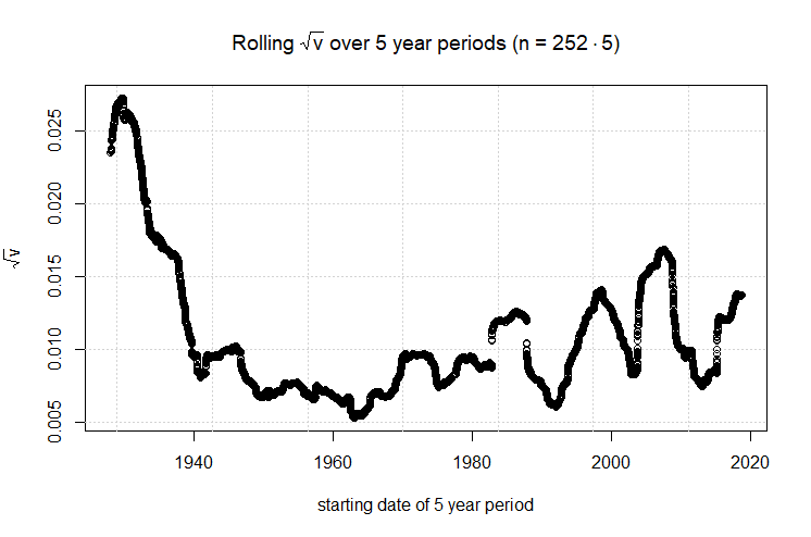
Figure 1: Recall (2). $\sqrt{v}$ measures the average volatility in daily returns of the underlying index.

Annual real returns of the S&P Composite Index from 1871 to 2020 are taken from http://www.econ.yale.edu/~shiller/data.html and collected for easy access at https://github.com/HaydenBrown/Investing. The S&P 500 only goes back to 1957, so Cowles and Associates (1871 to 1926) and the Standard & Poor 90 (1926 to 1957) are used as backward extensions. Relevant variables from the data are described in table 1.

Table 1: Data variable descriptions.

Notation	Description
$P$	average monthly close of the S&P composite index
$D$	dividend per share of the S&P composite index
$J$	January consumer price index

Inflation and dividend adjusted (i.e. real) annual returns are computed using the consumer price index, the S&P Composite Index price and the S&P Composite Index dividend. Use the subscript $k$ to denote the $k$th year of $J$, $P$ and $D$. Then the real return for year $k$ is given by $((P_{k+1}+D_{k})/P_{k})\cdot(J_{k}/J_{k+1})$. Figure 2 illustrates the remarkable stability of the S&P Composite Index real returns over the past 150 years. Supposing this stability continues, the long-term average annual log-return of the S&P 500 should be around .0658 plus the long-term average annual log-return of the consumer price index. Some possibilites are collected in table 2.

Table 2: Long-term average annual log-return for different inflation rates.

Long-term annual inflation	Long-term annual log-return
0%	.0658
1%	.0757
2%	.0856
3%	.0953
4%	.1050

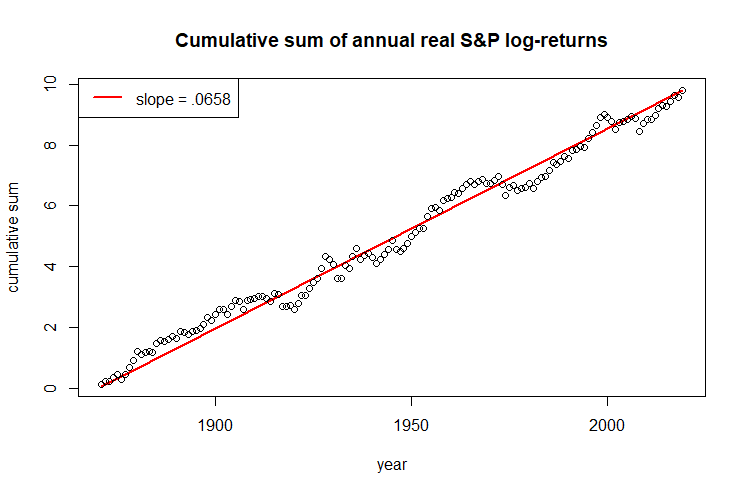
Figure 2: The cumulative sum of S&P Composite Index annual real log-returns is illustrated over 150 years. The slope of the linear trend is equal to the mean annual real log-return over that period.

3 Results

First some intuition is developed to show where results are coming from. Recall that the Maclaurin series representation for $\log(1+x)$ is given by

$$x-\frac{x^{2}}{2}+\frac{x^{3}}{3}-\frac{x^{4}}{4}+\ .\ .\ .\$$

When $x$ is sufficiently close to 0,

$$\log(1+x)\approx x-\frac{x^{2}}{2}.$$ (3)

Let $f:[0,\infty)\to\mathbb{R}$ be such that

$$f(x,y):=\log\frac{1-y/252}{1-x/252}.$$

Note that $f(x,y)=-f(y,x)$, and $f(x,y)\approx f(x-y,0)$.

If the compounded error is sufficiently small, then (1) and (3) imply

$$\begin{split}R_{n,r_{1}}^{L}-R_{n,r_{0}}^{1}&=\Big{[}\sum_{i=1}^{n}\log(1+LX_{i})-\log(1+X_{i})\Big{]}+n\cdot f(r_{0},r_{1})\\ &\approx\Big{[}\sum_{i=1}^{n}LX_{i}-\frac{(LX_{i})^{2}}{2}-\Big{(}X_{i}-\frac{X_{i}^{2}}{2}\Big{)}\Big{]}+n\cdot f(r_{0},r_{1})\\ &=(L-1)\Big{[}\sum_{i=1}^{n}X_{i}-\frac{L+1}{2}\cdot X_{i}^{2}\Big{]}+n\cdot f(r_{0},r_{1})\\ &\approx(L-1)\Big{[}\sum_{i=1}^{n}\log(1+X_{i})-\frac{L}{2}\cdot X_{i}^{2}\Big{]}+n\cdot f(r_{0},r_{1})\\ &=(L-1)\Big{[}R_{n,0}^{1}-\sum_{i=1}^{n}\frac{L}{2}\cdot X_{i}^{2}\Big{]}+n\cdot f(r_{0},r_{1}).\end{split}$$

It follows that

$$R_{n,r_{1}}^{L}-R_{n,r_{0}}^{1}\approx n[(L-1)(u-Lv/2)+f(r_{0},r_{1})].$$

So roughly speaking,

$$R_{n,r_{1}}^{L}\leq R_{n,r_{0}}^{1}\underset{\sim}{\iff}(L-1)(u-Lv/2)\leq f(r_{1},r_{0}).$$ (4)

Let $g:\mathbb{R}\to\mathbb{R}$ be such that

$$g(L):=(L-1)(u-Lv/2).$$

Observe that

$$\frac{\partial}{\partial L}g(L)=u+(1-2L)v/2.$$

Assuming $v>0$, it follows that the global maximum of $g$ is

$$\frac{v}{2}\Big{(}\frac{u}{v}-\frac{1}{2}\Big{)}^{2}.$$ (5)

and it occurs at $L=u/v+1/2$. Figure 3 shows how the optimal leverage multiple is affected by volatility and inflation.

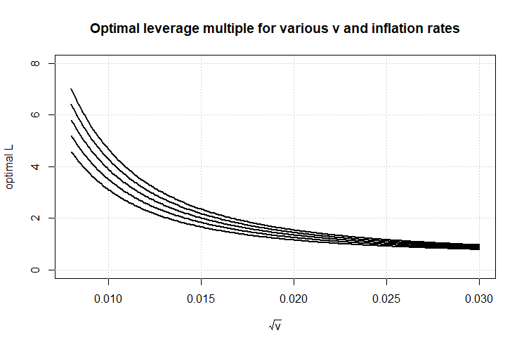
Figure 3: Illustrates $L=u/v+1/2$, which maximizes $g$. The $u$ are computed using table 2. For example, if the annual inflation rate is 2%, then $u=.0856/252$. Each curve corresponds to an inflation rate in table 2. More specifically, the curves (from top to bottom) correspond to annual inflation rates of 4%, 3%, 2%, 1% and 0%.

Let $h:(0,\infty)\to[0,\infty)$ be such that $h(v)$ is given by (5). Then

$$\frac{\partial}{\partial v}h(v)=-\frac{1}{2}\Big{(}\frac{u^{2}}{v^{2}}-\frac{1}{4}\Big{)}.$$

It follows that the global minimum of $h$ is

$$\begin{cases}0&u\geq 0\\ v/2&u<0\end{cases},$$

and it occurs at $v=2|u|$. Moreover, $h$ is decreasing for $v<2|u|$ and increasing for $v>2|u|$.

Next, the goal is to determine the $v$ such that $h(v)\leq f(r_{1},r_{0})$. Performing some algebra and then applying the quadratic formula,

$$\begin{split}h(v)=f(r_{1},r_{0})&\iff\sqrt{\frac{v}{2}}\cdot\Big{|}\frac{u}{v}-\frac{1}{2}\Big{|}=\sqrt{f(r_{1},r_{0})}\\ &\iff\Big{|}u-\frac{v}{2}\Big{|}=\sqrt{2v\cdot f(r_{1},r_{0})}\\ &\iff\mp\frac{1}{2}\cdot v-\sqrt{2f(r_{1},r_{0})}\cdot\sqrt{v}\pm u=0\\ &\iff v=2\big{(}\sqrt{f(r_{1},r_{0})}\pm\sqrt{f(r_{1},r_{0})+u}\ \big{)}^{2}.\end{split}$$

Let $v^{-}$ and $v^{+}$ be such that

$$v^{\pm}=2\big{(}\sqrt{f(r_{1},r_{0})}\pm\sqrt{f(r_{1},r_{0})+u}\ \big{)}^{2}.$$

Then

$$h(v)\leq f(r_{1},r_{0})\iff v\in[v^{-},v^{+}].$$ (6)

Figure 4 illustrates $v^{-}$ and $v^{+}$ for various $u$ and $r_{1}-r_{0}$. Note that $v^{-}$ and $v^{+}$ are undefined when $u<f(r_{0},r_{1})$, in which case $h(v)>f(r_{1},r_{0})$ for all $v>0$.

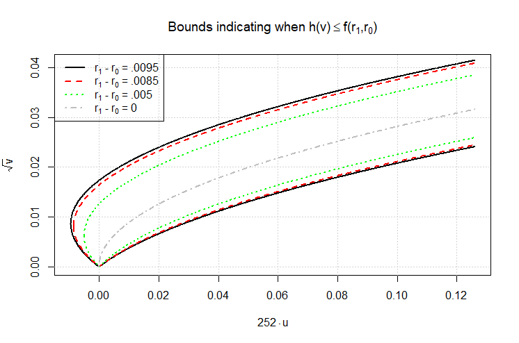
Figure 4: Recall (6). $\sqrt{v^{+}}$ and $\sqrt{v^{-}}$ are the top and bottom curves, respectively. Only one curve is shown for $r_{1}-r_{0}=0$ because $v^{+}=v^{-}$. Note that $f(r_{1},r_{0})\approx f(r_{1}-r_{0},0)$, so different combinations of $r_{1}$ and $r_{0}$ can be identified using their difference instead. The average annualized log-return is given by $252\cdot u$.

Now to confront these theoretical results with the S&P 500 data. First, (4) is justified by checking if

$$R_{n,r_{1}}^{L}-R_{n,r_{0}}^{1}\leq 0\underset{\sim}{\iff}(L-1)(u-Lv/2)\leq 0.$$ (7)

for various $L$ and $n$. Figure 5 illustrates the accuracy of (7) for some common leverage multiples $L$. Overall, there are very few instances where (7) does not hold strictly, i.e. where

$$(R_{n,0}^{L}-R_{n,0}^{1})\cdot n\cdot g(L)<0.$$

In those instances, Figure 5 shows that the error tends to be quite small. So (7) appears to be supported by the historical S&P 500 data.

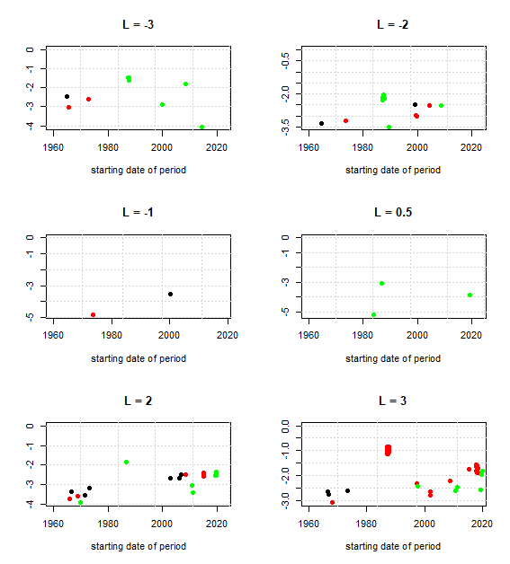
Figure 5: Illustrates rolling

$$\log_{10}(\max\{|R_{n,0}^{L}-R_{n,0}^{1}|,|n\cdot g(L)|\})$$

for various $L$ and $n$, but only when

$$(R_{n,0}^{L}-R_{n,0}^{1})\cdot n\cdot g(L)<0.$$

Green, red and black indicate periods of 1 ($n=252\cdot 1$), 5 ($n=252\cdot 5$) and 10 ($n=252\cdot 10$) years, respectively.

Theoretical results are entirely predicated on (7), and now that (7) has been validated for the S&P 500, it is possible to draw some conclusions. If market forces determine volatility such that a daily leveraged S&P 500 ETF cannot outperform its unleveraged counterpart in the long run, then table 2 and figure 4 combine to imply the long-term volatility of daily returns, measured as $\sqrt{v}$, should be at least .0158. Persistent inflation or a decrease in the difference between leveraged versus unleveraged ETF fees could bring this long-term volatility to startling levels, say beyond .02. Looking at figure 1, there appears to be room for a noticeable increase in daily volatility, provided the above hypothesis about market forces determining volatility is valid.

4 Conclusion

If daily volatiltiy continues to increase, eventually passing the necessary threshold, then leveraged S&P 500 ETFs will become obsolete for long-term investment. If daily volatility remains below this threshold, there will be opportunity for leveraged S&P 500 ETFs to beat standard S&P 500 ETFs. However, it may be difficult to take advantage of these opportunities if future daily volatility becomes difficult to predict, especially if no noticeable correlation exists between expected daily log-return and daily volatility.

The focus here was on the S&P 500 because of its historic stability. Other indexes may also produce decent results. However, any meaningful application will need a sufficiently accurate prediction of the mean daily log-return for the period in question. Examples include an upper or lower bound on the mean that is anticipated to hold with high confidence. If such a prediction is not obtainable, then it may be wise to avoid any leveraged ETF based on that index.

As identified in Washer et al (2016), there is an interesting phenomenon occurring where daily volatility increases, but volatility of returns over a longer period, say monthly, does not. This is not how returns should behave if daily returns are generally independent and identically distributed. Future research could investigate what sort of stochastic processes can exhibit increased short-term volatility while maintaining long-term volatility.

References

- \bibcommenthead
- Ben-David et al (2018) Ben-David I, Franzoni F, Moussawi R (2018) Do etfs increase volatility? The Journal of Finance 73(6):2471–2535
- Brown (2023) Brown H (2023) Long-term returns estimation of leveraged indexes and etfs. Financial Markets and Portfolio Management
- Conrad and Loch (2015) Conrad C, Loch K (2015) Anticipating long-term stock market volatility. Journal of Applied Econometrics 30(7):1090–1114
- Perron and Qu (2010) Perron P, Qu Z (2010) Long-memory and level shifts in the volatility of stock market return indices. Journal of Business & Economic Statistics 28(2):275–290
- Washer et al (2016) Washer KM, Jorgensen R, Johnson RR (2016) The increasing volatility of the stock market? The Journal of Wealth Management 19(1):71–82