Coupled cluster theory for nonadiabatic dynamics: nuclear gradients and nonadiabatic couplings in similarity constrained coupled cluster theory

Abstract

Coupled cluster theory is one of the most accurate electronic structure methods for predicting ground and excited state chemistry. However, the presence of numerical artifacts at electronic degeneracies, such as complex energies, has made it difficult to apply it in nonadiabatic dynamics simulations. While it has already been shown that such numerical artifacts can be fully removed by using similarity constrained coupled cluster (SCC) theory [J. Phys. Chem. Lett. 2017, 8, 19, 4801–4807], simulating dynamics requires efficient implementations of gradients and nonadiabatic couplings. Here, we present an implementation of nuclear gradients and nonadiabatic derivative couplings at the similarity constrained coupled cluster singles and doubles (SCCSD) level of theory. We present a few numerical examples that show good agreement with literature values and discuss some limitations of the method. In a separate paper, we show that this implementation can be used in nonadiabatic dynamics, thereby establishing coupled cluster theory as a viable electronic structure method for simulating excited state photochemistry.

I Introduction

Upon photoexcitation to an excited electronic state, molecular systems normally undergo relaxation through one or more conical intersections. When a system reaches such electronic degeneracies, the dynamics of the nuclei changes: the nuclear motion must then be treated in terms of a nuclear wavepacket and the coupling between the electrons and the nuclei (nonadiabatic coupling) becomes large, leading to a breakdown of the Born-Oppenheimer approximation. As a result, non-radiative transfer of nuclear population between electronic states becomes possible, something that typically occurs within tens or hundreds of femtoseconds after excitation by light.[1]

It is challenging to simulate such a process, however, as it requires an accurate treatment not only of the nuclear wavepacket but also of the electronic states involved. The choice of the electronic structure method often qualitatively alters the predicted dynamics, emphasizing the importance of a balanced and accurate treatment of the electronic states.[2] Depending on the system of interest, it can be important to effectively capture static correlation (for example, by using complete active space methods[3]) or dynamical correlation (for example, by using density functional theory[4]). In the latter category, coupled cluster theory[5, 6] is often particularly accurate,[7] making it a promising candidate for simulating photochemical processes.

A major theoretical issue has hindered this, however. Coupled cluster methods are known to produce numerical artifacts at same-symmetry conical intersections, where the potential energy surfaces become distorted and the energies can become complex-valued. This fact led some authors[8, 9] to question whether the method could be used to simulate excited state dynamics. As was recently shown by the authors and collaborators, however, the numerical artifacts of the method can be removed by constraining the electronic states to be orthogonal, which furthermore implies a correct intersection dimensionality (two directions lift the degeneracy) and a proper first-order behavior as the degeneracy is lifted (the intersections are conical).[10, 11, 12] These developments indicated that the modified coupled cluster method, known as similarity constrained coupled cluster (SCC)[11, 12] theory, would be applicable in excited state nonadiabatic dynamics simulations.

Large-scale simulations require efficient implementations of the nuclear energy gradients and the nonadiabatic derivative coupling elements. In the case of coupled cluster energy gradients, both derivation techniques and efficient implementations are well-established and widespread.[13, 14, 15, 16] Less attention has been given to the nonadiabatic couplings. There have been two recent implementations at the coupled cluster singles and doubles level of theory (CCSD), although these arrive at the coupling elements through two different routes: one evaluates the couplings in terms of summed-state gradients[17, 18] while the other (implemented by the authors) directly evaluates them by using standard Lagrangian/Z-vector techniques.[19, 20] There is some uncertainty about whether these are equivalent.[20]

In this paper, we derive and implement analytical derivative couplings and energy gradients for the similarity constrained coupled cluster singles and doubles (SCCSD)[12] method, building on our recent CCSD implementations of analytical derivative coupling elements[20] and nuclear energy gradients.[21] Here we will focus on implementation aspects. In a separate paper, we use the implementation to perform the first nonadiabatic dynamics simulations at the CCSD and SCCSD levels.[22] By applying SCCSD whenever CCSD encounters numerical artifacts, we obtain a correct description of conical intersections in the dynamics. This separate study correctly predicts the experimental time constant for the ultrafast $\pi\pi^{\ast}$/$n\pi^{\ast}$ conversion in thymine upon photoexcitation to the $\pi\pi^{\ast}$ state, demonstrating that coupled cluster theory can be predictive in nonadiabatic dynamics.[22]

II Theory

II.1 Coupled cluster theory

In coupled cluster theory, the ground state wave function is written as[23, 24]

$$|\psi_{0}\rangle=\exp(\mathscr{T})|\mathrm{HF}\rangle,$$ (1)

where $\mathscr{T}$ is called the cluster operator and the reference wave function $|\mathrm{HF}\rangle$ is usually taken to be the Hartree-Fock state. By applying the exponential operator, the mean-field wave function $|\mathrm{HF}\rangle$ is transformed into a correlated wave function $|\psi_{0}\rangle$ that more accurately represents the electronic ground state.

In practice, the cluster operator incorporates excitations only up to a given rank. For instance, it may include single and double excitations with respect to $|\mathrm{HF}\rangle$, in which case we obtain the coupled cluster with singles and doubles (CCSD)[25] method. More generally, the cluster operator is written

$$\mathscr{T}=\sum_{\mu\in\mathscr{E}_{e}}t_{\mu}\tau_{\mu}=T_{1}+T_{2}+\ldots+T_{n},$$ (2)

where $\mathscr{E}_{e}$ denotes the included excitations, the subscript $k$ in $T_{k}$ denotes the excitation rank, and the sum truncates at a given excitation order $n$. For example, $\mathscr{T}=T_{1}+T_{2}$ in CCSD. Each excitation operator $\tau_{\mu}$ is weighted by an amplitude $t_{\mu}$, and this amplitude indicates the weight in $|\psi_{0}\rangle$ of the associated configuration $|\mu\rangle=\tau_{\mu}|\mathrm{HF}\rangle$.

These cluster amplitudes are determined by projecting the Schrödinger equation onto the excitation subspace $\mathscr{E}_{e}$. We start from the Schrödinger equation for $|\psi_{0}\rangle$,

$$H|\psi_{0}\rangle=E_{0}|\psi_{0}\rangle,$$ (3)

where $H$ denotes the electronic Hamiltonian, $|\psi_{0}\rangle$ is given in Eq. (1), and $E_{0}$ is the ground state energy. Next, we project the Schrödinger equation onto

$$\begin{split}\{\langle\mathrm{HF}|\exp(-\mathscr{T}),\langle\mu|\exp(-\mathscr{T})\},\end{split}$$ (4)

where $\mu\in\mathscr{E}_{e}$. This projection procedure gives a set of equations that determine $E_{0}$ and $t_{\mu}$:

$$E_{0} =\langle\mathrm{HF}|\bar{H}|\mathrm{HF}\rangle$$ (5)

$$0 =\langle\mu|\bar{H}|\mathrm{HF}\rangle=\Omega_{\mu},$$ (6)

where

$$\bar{H}=\exp(-\mathscr{T})H\exp(\mathscr{T}),$$ (7)

If we want to make the orbital dependence explicit, we can also write[26]

$$\bar{H}=\exp(-\mathscr{T})\exp(\kappa)H\exp(-\kappa)\exp(\mathscr{T}),$$ (8)

where the orbital rotation operator is given by

$$\kappa=\sum_{ai}\kappa_{ai}(E_{ai}-E_{ia})=\sum_{ai}\kappa_{ai}E_{ai}^{-}.$$ (9)

Here, $E_{ai}$ is the singlet excitation operator from the occupied orbital $i$ to the virtual orbital $a$. In calculations at a specific geometry, $\kappa=0$ is normally understood to correspond to the Hartree-Fock orbitals, and we write $\bar{H}$ as in Eq. (7). When we evaluate nuclear gradients, we need the latter form, Eq. (8), as $\kappa$ will be different from zero when we make displacements away from the geometry where we evaluate the gradient.

A peculiar feature of coupled cluster theory, which stems from the non-Hermiticity of $\bar{H}$, is the introduction of left (or bra) states that are different from the right (or ket) states. In particular, $|\psi_{0}\rangle^{\dagger}\neq\langle\psi_{0}|$. The left ground state does not have an exponential form, like in Eq. (1), but is instead expressed as

$$\langle\psi_{0}|=\Bigl{(}\langle\mathrm{HF}|+\sum_{\mu\in\mathscr{E}_{e}}\bar{t}_{\mu}\langle\mu|\Bigr{)}\exp(-\mathscr{T}).$$ (10)

Nonetheless, like $|\psi_{0}\rangle$, it is also determined by projecting the Schrödinger equation. Starting from

$$\langle\psi_{0}|H=\langle\psi_{0}|E_{0},$$ (11)

we project onto

$$\{\exp(\mathscr{T})|\mathrm{HF}\rangle,\exp(\mathscr{T})|\mu\rangle\},$$ (12)

where $\mu\in\mathscr{E}_{e}$. This results in an equation for $\bar{t}_{\mu}$:[27]

$$0=\langle\mathrm{HF}\hskip 1.00006pt|\hskip 1.00006pt[\bar{H},\tau_{\mu}]\hskip 1.00006pt|\hskip 1.00006pt\mathrm{HF}\rangle+\sum_{\nu\in\mathscr{E}_{e}}\bar{t}_{\nu}\langle\nu\hskip 1.00006pt|\hskip 1.00006pt[\bar{H},\tau_{\mu}]\hskip 1.00006pt|\hskip 1.00006pt\mathrm{HF}\rangle.$$ (13)

Once $\langle\psi_{0}|$ and $|\psi_{0}\rangle$ are known, we can evaluate molecular properties by substituting these wave functions into known exact expressions. The dipole moment, for example, can be evaluated as $\langle\psi_{0}\hskip 1.00006pt|\hskip 1.00006pt\hat{\mu}\hskip 1.00006pt|\hskip 1.00006pt\psi_{0}\rangle$, where $\langle\psi_{0}|$ is given by Eq. (10) and $|\psi_{0}\rangle$ is given by Eq. (1).

The excited states can be described with two alternative but closely related approaches, the linear response[5] and equation of motion theories.[6] In the equation of motion approach, which we adopt here, the excited states are expressed as

$$|\psi_{n}\rangle =\exp(\mathscr{T})\Bigl{(}R_{0}^{n}|\mathrm{HF}\rangle+\sum_{\mu\in\mathscr{E}_{e}}R_{\mu}^{n}|\mu\rangle\Bigr{)}$$ (14)

$$\langle\psi_{n}| =\Bigl{(}L_{0}^{n}\langle\mathrm{HF}|+\sum_{\mu\in\mathscr{E}_{e}}L_{\mu}^{n}\langle\mu|\Bigr{)}\exp(-\mathscr{T}),$$ (15)

and these states are determined by the same projection procedure used for the ground state. It will be convenient to define $|0\rangle=|\mathrm{HF}\rangle$ so that $\mu=0$ corresponds to the reference state and $\tau_{0}=1$. Then, if we let $\mathscr{E}$ denote the set containing both $\mu=0$ and $\mu\in\mathscr{E}_{e}$, we can write

$$|\psi_{n}\rangle =\exp(\mathscr{T})\Bigl{(}\sum_{\mu\in\mathscr{E}}R_{\mu}^{n}|\mu\rangle\Bigr{)}$$ (16)

$$\langle\psi_{n}| =\Bigl{(}\sum_{\mu\in\mathscr{E}}L_{\mu}^{n}\langle\mu|\Bigr{)}\exp(-\mathscr{T}).$$ (17)

When we repeat the ground state projection procedure for the excited states, we find that the excited state amplitudes satisfy eigenvalue equations,

$$\bar{\bm{\mathcal{H}}}\bm{\mathcal{R}}_{n} =E_{n}\bm{\mathcal{R}}_{n}$$ (18)

$$\bm{\mathcal{L}}_{n}^{\mathrm{T}}\bar{\bm{\mathcal{H}}} =E_{n}\bm{\mathcal{L}}_{n}^{\mathrm{T}},$$ (19)

where

$$\bar{\mathcal{H}}_{\mu\nu}=\langle\mu\hskip 1.00006pt|\hskip 1.00006pt\bar{H}\hskip 1.00006pt|\hskip 1.00006pt\nu\rangle,\quad\mu,\nu\in\mathscr{E}$$ (20)

and

$$\bm{\mathcal{R}}_{n}=\begin{pmatrix}R_{n}^{0}\\ \bm{R}_{n}\end{pmatrix},\quad\bm{\mathcal{L}}_{n}^{\mathrm{T}}=\begin{pmatrix}L_{n}^{0}\;\bm{L}_{n}^{\mathrm{T}}\end{pmatrix}.$$ (21)

Here, $E_{n}$, with $n=1,2,\ldots$, denotes the excited state energy. Note also that the ground state wave functions satisfy the same eigenvalue equations, with vectors given as

$$\bm{\mathcal{R}}_{0}=\begin{pmatrix}1\\ \bm{0}\end{pmatrix},\quad\bm{\mathcal{L}}_{0}^{\mathrm{T}}=\begin{pmatrix}1\;\bar{\bm{t}}^{\mathrm{T}}\end{pmatrix}.$$ (22)

Once $\langle\psi_{n}|$ and $|\psi_{n}\rangle$ have been determined, we can evaluate molecular properties by substitution into the exact expression for the given property. For example, the nuclear gradient of the energy can be evaluated as

$$\bm{g}_{n}=\nabla\langle\psi_{n}\hskip 1.00006pt|\hskip 1.00006ptH\hskip 1.00006pt|\hskip 1.00006pt\psi_{n}\rangle$$ (23)

and the nonadiabatic derivative coupling vector as

$$\bm{d}_{mn}=\langle\psi_{m}\hskip 1.00006pt|\hskip 1.00006pt\nabla\psi_{n}\rangle.$$ (24)

These two quantities, $\bm{g}_{n}$ and $\bm{d}_{mn}$, are of special interest in molecular dynamics. The gradient $\bm{g}_{n}$ provides the force acting on the nuclei, while the derivative coupling $\bm{d}_{mn}$ is responsible for nonadiabatic transitions between electronic states.

The derivative coupling vector diverges at conical intersections, where the electronic states are degenerate. This is easily seen in the exact limit, where we have

$$\bm{d}_{mn}=\langle\psi_{m}\hskip 1.00006pt|\hskip 1.00006pt\nabla\psi_{n}\rangle=\frac{\langle\psi_{m}\hskip 1.00006pt|\hskip 1.00006pt(\nabla H)\psi_{n}\rangle}{E_{m}-E_{n}}.$$ (25)

A proper description of such intersections is therefore essential if a method is to be applied in photochemical applications. Somewhat surprisingly, it turns out[10, 11, 12] that these intersections can only be described correctly if the method guarantees some sort of orthogonality between the excited states, something which is not true in standard coupled cluster theory.

II.2 Similarity constrained coupled cluster theory

In similarity constrained coupled cluster theory, which was designed for applications to nonadiabatic dynamics,[10, 11, 12] a set of electronic states are constrained to be orthogonal. Here, a subset of states $\mathscr{K}$ satisfy

$$\mathscr{O}_{kl}=\langle\psi_{k}\hskip 1.00006pt|\hskip 1.00006pt\mathscr{P}\hskip 1.00006pt|\hskip 1.00006pt\psi_{l}\rangle=0,\quad k\neq l\in\mathscr{K},$$ (26)

where $\mathscr{P}$ is a projection operator and so $\mathscr{O}_{kl}$ is an approximation of $\langle\psi_{k}\hskip 1.00006pt|\hskip 1.00006pt\psi_{l}\rangle$. To enforce the orthogonality of the states, the cluster operator is expressed as

$$\mathscr{T}=\sum_{\mu\in\mathscr{E}}t_{\mu}\tau_{\mu}+\sum_{k\neq l\in\mathscr{K}}\zeta_{kl}X_{kl},$$ (27)

where each $X_{kl}$ is an excitation operator whose rank is higher than the $\mu$ included in $\mathscr{E}$, and $\zeta_{kl}$ enforces $\mathscr{O}_{kl}=0$. Both $\mathscr{P}$ and $X_{kl}$ can be chosen in several different ways, leading to different variants of the theory.[11, 12] Here we will assume that they only depend on the right excited states,

$$\mathscr{P}=\mathscr{P}(\{\mathcal{R}_{n}\}),\quad X_{kl}=X_{kl}(\mathcal{R}_{k},\mathcal{R}_{l}),$$ (28)

as this is required for the method to scale correctly with the size of the system (that is, to be size-extensive/size-intensive).[12] The similarity constrained coupled cluster method can be considered an extension of the standard coupled cluster method, since all the standard equations are still kept unchanged. The only changes to the method are the additional orthogonality conditions $\mathscr{O}_{kl}=0$ and the additional excitation operators in $\mathscr{T}$. Note, however, that the orthogonality conditions couple the ground state to the excited states in $\mathscr{K}$, meaning that the ground and excited states must be determined simultaneously.

II.3 Nuclear gradients and derivative coupling elements

II.3.1 Lagrangians

As noted already, the nuclear gradients and derivative couplings are the two main components needed to simulate nonadiabatic excited state dynamics. We therefore need to know how to evaluate these elements efficiently in our approximate electronic structure methods. The generally adopted approach is to apply the Langragian method, also called the Z-vector method, which allows us to effectively evaluate gradients (for example, of the energy) by imposing a set of constraints on the parameters of the electronic structure method.[13, 14]

Its main advantage here is that it removes the need to explicitly evaluate the derivatives of these parameters, for example, $\mathrm{d}t_{\mu}/\mathrm{d}x$, where $x$ is a nuclear coordinate. These derivatives are instead accounted for through the constraints and the associated Lagrangian multipliers. If we assume that we want to evaluate the gradient of $E$ with respect to $\bm{x}$, where $E$ depends on a set of parameters $\bm{\lambda}$ that can be determined by solving a set of equations $\bm{e}=0$, then the Lagrangian takes the form

$$\mathscr{L}(\bm{\lambda},\bar{\bm{\lambda}},\bm{x})=E(\bm{\lambda},\bm{x})+\sum_{p}\bar{\lambda}_{p}e_{p}(\bm{\lambda},\bm{x}),$$ (29)

where $\bar{\bm{\lambda}}$ contains the so-called Lagrangian multipliers. The constraints ($\bm{e}=0$) are imposed by making the Lagrangian stationary with respect to the multipliers $\bar{\bm{\lambda}}$, while the multipliers are determined by making the Lagrangian stationary with respect to the parameters $\bm{\lambda}$. In other words, we have

$$\frac{\partial\mathscr{L}}{\partial\lambda_{p}}=0,\quad\frac{\partial\mathscr{L}}{\partial\bar{\lambda}_{p}}=e_{p}=0,$$ (30)

which implies that

$$\frac{\mathrm{d}E}{\mathrm{d}x}=\frac{\mathrm{d}\mathscr{L}}{\mathrm{d}x}=\frac{\partial\mathscr{L}}{\partial x}+\sum_{p}\frac{\partial\mathscr{L}}{\partial\lambda_{p}}\frac{\partial\lambda_{p}}{\partial x}=\frac{\partial\mathscr{L}}{\partial x}.$$ (31)

The total derivative of $E$ is replaced by the partial derivative of $\mathscr{L}$, and the latter contains no derivative of the parameters with respect to $\bm{x}$.

Our constraints are simply the equations that determine the parameters; for example, one set of constraints are the ground state equations $\Omega_{\mu}=0$, since these equations determine the amplitudes $t_{\mu}$. Each set of constraints is given a set of Lagrangian multipliers; for example, the ground state equations $\Omega_{\mu}=0$ are associated with a set of multipliers $\bar{\zeta}_{\mu}$. Written out explicitly, the nuclear gradient $\bm{g}_{n}$, where $n\in\mathscr{K}$, can be evaluated from the Lagrangian

$$\begin{split}\mathscr{L}_{n}&=E_{n}+\sum_{k\in\mathscr{K}}\langle\mathcal{\bar{L}}_{k}\hskip 1.00006pt|\hskip 1.00006pt\bar{H}-E_{k}\hskip 1.00006pt|\hskip 1.00006pt\mathcal{R}_{k}\rangle\\ &+\sum_{k\in\mathscr{K}}\bar{E}_{k}(1-\langle\Lambda_{k}\hskip 1.00006pt|\hskip 1.00006ptR_{k}\rangle)+\sum_{k\neq l\in\mathscr{K}}\bar{\gamma}_{kl}\mathscr{O}_{kl}+\sum_{\mu}\bar{\zeta}_{\mu}\Omega_{\mu}+\sum_{ai}\bar{\kappa}_{ai}F_{ai},\end{split}$$ (32)

where $F$ denotes the Fock matrix, $a$ and $i$ denote a virtual and an occupied orbital, respectively, and

$$E_{k}=\langle\Lambda_{k}\hskip 1.00006pt|\hskip 1.00006pt\bar{H}\hskip 1.00006pt|\hskip 1.00006ptR_{k}\rangle$$ (33)

is the energy of state $k$. Here, $\langle\Lambda_{k}|$ is some (for now unspecified) vector that is normalized with respect to $|R_{k}\rangle$, that is, $\langle\Lambda_{k}\hskip 1.00006pt|\hskip 1.00006ptR_{k}\rangle=1$. Note that Eq. (33) will then be equal to the energy as a result of the eigenvalue equation in Eq. (18). The first term in $\mathscr{L}_{n}$ is the energy, and the rest are the Lagrangian constraints. The first and second constraints ensure that the states in $\mathscr{K}$ are eigenstates and that $E_{k}$ is the energy of the $k$th state, while the third ensures that the states in $\mathscr{K}$ are orthogonal (that is, $\mathscr{O}_{kl}=0$ for $k\neq l\in\mathscr{K}$). The final two constraints are the ground state coupled cluster equations and the Hartree-Fock equations, which respectively determine the cluster amplitudes $t_{\mu}$ and the molecular orbitals.

The Lagrangian for the derivative couplings is identical to that for the nuclear gradient (because the constraints $\bm{e}=0$ are the same), except for the first term. The coupling $\bm{d}_{mn}$ between $m,n\in\mathscr{K}$ can be evaluated from

$$\begin{split}\mathscr{L}_{mn}&=O_{mn}+\sum_{k\in\mathscr{K}}\langle\mathcal{\bar{L}}_{k}\hskip 1.00006pt|\hskip 1.00006pt\bar{H}-E_{k}\hskip 1.00006pt|\hskip 1.00006pt\mathcal{R}_{k}\rangle\\ &+\sum_{k\in\mathscr{K}}\bar{E}_{k}(1-\langle\Lambda_{k}\hskip 1.00006pt|\hskip 1.00006ptR_{k}\rangle)+\sum_{k\neq l\in\mathscr{K}}\bar{\gamma}_{kl}\mathscr{O}_{kl}+\sum_{\mu}\bar{\zeta}_{\mu}\Omega_{\mu}+\sum_{ai}\bar{\kappa}_{ai}F_{ai},\end{split}$$ (34)

where we define the bra-frozen overlap, as proposed by Hohenstein,[28] as

$$O_{mn}=\langle\psi_{m}(\bm{x}_{0})\hskip 1.00006pt|\hskip 1.00006pt\psi_{n}(\bm{x})\rangle.$$ (35)

Here, $O_{mn}$ introduces a parametric dependence on some reference geometry $\bm{x}_{0}$. This means that this Lagrangian can be used to evaluate the coupling exactly at $\bm{x}_{0}$ and not at any other values of $\bm{x}$. However, since $\bm{x}_{0}$ can be chosen freely, this implies no loss of generality.

II.3.2 Expressions for the gradient and couplings

Once the multipliers are known, we can evaluate the gradients and couplings as

$$\bm{g}_{n} =\nabla E_{n}=\frac{\mathrm{d}E_{n}}{\mathrm{d}\bm{x}}=\frac{\partial\mathscr{L}_{n}}{\partial\bm{x}}$$ (36)

and

$$\bm{d}_{mn} =\langle\psi_{m}\hskip 1.00006pt|\hskip 1.00006pt\nabla\psi_{n}\rangle=\Big{\langle}\psi_{m}\hskip 1.00006pt\Big{|}\hskip 1.00006pt\frac{\mathrm{d}\psi_{n}}{\mathrm{d}\bm{x}}\Big{\rangle}=\frac{\partial\mathscr{L}_{mn}}{\partial\bm{x}}.$$ (37)

Let us write out the gradient expression in detail. When taking the partial derivative of the Lagrangian, we can treat the parameters as constants as their dependence on the nuclear coordinates is included in the multiplier terms. In addition, the dependence of the creation and annihilation operators on $\bm{x}$ can be ignored, see Ref. 14. Thus, the only explicit nuclear dependence resides in the Hamiltonian integrals. We denote the nuclear derivatives $\{\partial H/\partial x_{q}|_{0}\}$ as $H^{(1)}$ and let

$$\bar{H}^{(1)}=\exp(-\mathscr{T})\exp(\kappa)H^{(1)}\exp(-\kappa)\exp(\mathscr{T}),$$ (38)

where $\kappa=0$ corresponds to the Hartree-Fock orbitals at $\bm{x}_{0}$. Since the derivative only acts on the Hamiltonian, it is convenient to introduce some further notation. In particular, if we let

$$\begin{split}\langle K_{k}|&=(\delta_{kn}-\langle\bar{\mathcal{L}}_{k}\hskip 1.00006pt|\hskip 1.00006pt\mathcal{R}_{k}\rangle)\langle\Lambda_{k}|+\langle\bar{L}_{k}|,\end{split}$$ (39)

the Lagrangian becomes

$$\begin{split}\mathscr{L}_{n}&=\sum_{k\in\mathscr{K}}(\langle K_{k}\hskip 1.00006pt|\hskip 1.00006pt\bar{H}\hskip 1.00006pt|\hskip 1.00006ptR_{k}\rangle+\bar{L}_{0}^{k}\langle\mathrm{HF}\hskip 1.00006pt|\hskip 1.00006pt\bar{H}\hskip 1.00006pt|\hskip 1.00006pt\mathcal{R}_{k}\rangle)\\ &\quad+\langle\bar{\zeta}\hskip 1.00006pt|\hskip 1.00006pt\bar{H}\hskip 1.00006pt|\hskip 1.00006pt\mathrm{HF}\rangle+\sum_{ai}\bar{\kappa}_{ai}F_{ai}\\ &\quad+\sum_{k\in\mathscr{K}}\bar{E}_{k}(1-\langle\Lambda_{k}\hskip 1.00006pt|\hskip 1.00006ptR_{k}\rangle)+\sum_{k\neq l\in\mathscr{K}}\bar{\gamma}_{kl}\mathscr{O}_{kl}\end{split}$$ (40)

and the nuclear gradient becomes

$$\begin{split}\bm{g}_{n}&=\mathscr{L}_{n}^{(1)}=\sum_{k\in\mathscr{K}}(\langle K_{k}\hskip 1.00006pt|\hskip 1.00006pt\bar{H}^{(1)}\hskip 1.00006pt|\hskip 1.00006ptR_{k}\rangle+\bar{L}_{0}^{k}\langle\mathrm{HF}\hskip 1.00006pt|\hskip 1.00006pt\bar{H}^{(1)}\hskip 1.00006pt|\hskip 1.00006pt\mathcal{R}_{k}\rangle)\\ &\quad\quad\quad\quad\quad\quad+\langle\bar{\zeta}\hskip 1.00006pt|\hskip 1.00006pt\bar{H}^{(1)}\hskip 1.00006pt|\hskip 1.00006pt\mathrm{HF}\rangle+\sum_{ai}\bar{\kappa}_{ai}F_{ai}^{(1)}.\end{split}$$ (41)

Note that, when we apply the derivative, the last two terms in $\mathscr{L}_{n}$ vanish because there is no $H$-dependence in these terms and so the partial derivatives are zero. The expression for $\bm{g}_{n}$ found here is similar to the standard coupled cluster case,[21] except that there are additional excited state terms which appear due to the coupling of states in $\mathscr{K}$ that arises due to the orthogonality conditions (in this case, the $\langle K_{k}|$ and $\bar{L}^{k}_{0}$ terms with $k\neq n$).

The expression for the derivative coupling is similar. In particular, we find that

$$\begin{split}\bm{d}_{mn}=\mathscr{L}_{mn}^{(1)}&=O_{mn}^{(1)}+\sum_{k\in\mathscr{K}}(\langle K_{k}\hskip 1.00006pt|\hskip 1.00006pt\bar{H}^{(1)}\hskip 1.00006pt|\hskip 1.00006ptR_{k}\rangle+\bar{L}_{0}^{k}\langle\mathrm{HF}\hskip 1.00006pt|\hskip 1.00006pt\bar{H}^{(1)}\hskip 1.00006pt|\hskip 1.00006pt\mathcal{R}_{k}\rangle)\\ &\quad\quad+\langle\bar{\zeta}\hskip 1.00006pt|\hskip 1.00006pt\bar{H}^{(1)}\hskip 1.00006pt|\hskip 1.00006pt\mathrm{HF}\rangle+\sum_{ai}\bar{\kappa}_{ai}F_{ai}^{(1)},\end{split}$$ (42)

where we instead have

$$\langle K_{k}|=-\langle\bar{\mathcal{L}}_{k}\hskip 1.00006pt|\hskip 1.00006pt\mathcal{R}_{k}\rangle\langle\Lambda_{k}|+\langle\bar{L}_{k}|.$$ (43)

Both $\bm{g}_{n}$ and $\bm{d}_{mn}$ consist of several terms that are transition elements of the gradient Hamiltonian $\bar{H}^{(1)}$. These are conveniently calculated in terms of density matrices, which we can write, for general $\langle\mathcal{L}|$ and $|\mathcal{R}\rangle$ vectors, as

$$\langle\mathcal{L}\hskip 1.00006pt|\hskip 1.00006pt\bar{H}^{(1)}\hskip 1.00006pt|\hskip 1.00006pt\mathcal{R}\rangle=\sum_{pq}h_{pq}^{(1)}d_{pq}(\bm{\mathcal{L}},\bm{\mathcal{R}})+\frac{1}{2}\sum_{pqrs}g_{pqrs}^{(1)}d_{pqrs}(\bm{\mathcal{L}},\bm{\mathcal{R}})+\langle\mathcal{L}\hskip 1.00006pt|\hskip 1.00006pt\mathcal{R}\rangle h_{\mathrm{nuc}}^{(1)},$$ (44)

where

$$d_{pq}(\bm{\mathcal{L}},\bm{\mathcal{R}}) =\langle\mathcal{L}\hskip 1.00006pt|\hskip 1.00006pt\exp(-\mathscr{T})E_{pq}\exp(\mathscr{T})\hskip 1.00006pt|\hskip 1.00006pt\mathcal{R}\rangle$$ (45)

$$d_{pqrs}(\bm{\mathcal{L}},\bm{\mathcal{R}}) =\langle\mathcal{L}\hskip 1.00006pt|\hskip 1.00006pt\exp(-\mathscr{T})e_{pqrs}\exp(\mathscr{T})\hskip 1.00006pt|\hskip 1.00006pt\mathcal{R}\rangle,\quad e_{pqrs}=E_{pq}E_{rs}+\delta_{qr}E_{ps},$$ (46)

and where we have used that the Hamiltonian can be expressed as

$$H=\sum_{pq}h_{pq}E_{pq}+\frac{1}{2}\sum_{pqrs}g_{pqrs}e_{pqrs}+h_{\mathrm{nuc}}.$$ (47)

In the above equations, $h_{pq}$ and $g_{pqrs}$ denote the one- and two-electron Hamiltonian integrals, respectively, and $h_{\mathrm{nuc}}$ denotes the nuclear repulsion energy. The indices $p,q,r,$ and $s$ denote general molecular orbitals.

II.3.3 Stationarity equations: nuclear gradient

As noted above, evaluating the gradient and couplings is only possible after we have determined the Lagrangian multipliers. Let us begin with the gradient Lagrangian $\mathscr{L}_{n}$. The multipliers are determined from the stationarity equations, which involve derivatives with respect to the orbital rotation parameters, $\kappa_{ai}$, the cluster amplitudes, $t_{\mu}$, and the excited state amplitudes, $R_{\mu}^{k}$ and $\zeta_{kl}$. Below, we derive expressions for these stationarity equations.

It turns out that the stationarity equations have a simpler form if the lambda states, $\langle\Lambda_{k}|$, at $\bm{x}_{0}$, are chosen to be equal to the left excited state vectors, that is, if

$$\langle\Lambda_{k}|=\langle L_{k}|,$$ (48)

and we will assume this in the remainder of the text. Let us start by considering stationarity with respect to the lambda states, which will allow us to determine the multipliers $\bar{E}_{m}$. In fact, since

$$\frac{\partial\mathscr{L}_{n}}{\partial\Lambda_{\mu}^{m}}\Big{|}_{0}=0=R_{\mu}^{m}\Big{\{}E_{m}(\delta_{mn}-\langle\mathscr{\bar{L}}_{m}\hskip 1.00006pt|\hskip 1.00006pt\mathscr{R}_{m}\rangle)-\bar{E}_{m}\Big{\}},$$ (49)

we can ensure stationarity by setting

$$\bar{E}_{m}=E_{m}(\delta_{mn}-\langle\mathscr{\bar{L}}_{m}\hskip 1.00006pt|\hskip 1.00006pt\mathscr{R}_{m}\rangle).$$ (50)

In addition, it turns out that the multipliers relating to the Hartree-Fock contribution to the excited states, that is, $\bar{L}^{k}_{0}$, can be expressed in terms of the orthogonality multipliers $\bar{\gamma}_{kl}$. In particular, we have

$$\frac{\partial\mathscr{L}_{n}}{\partial R_{0}^{m}}\Big{|}_{0}=0=-\omega_{m}\bar{L}_{0}^{m}+\sum_{k\neq l\in\mathscr{K}}\bar{\gamma}_{kl}\frac{\partial\mathscr{O}_{kl}}{\partial R_{0}^{m}},$$ (51)

where $\omega_{m}=E_{m}-E_{0}$, and, therefore,

$$\bar{L}_{0}^{m}=\sum_{k\neq l\in\mathscr{K}}\bar{\gamma}_{kl}\Bigl{(}\frac{1}{\omega_{m}}\frac{\partial\mathscr{O}_{kl}}{\partial R_{0}^{m}}\Bigr{)}.$$ (52)

The remaining multipliers ($\bm{\bar{\zeta}},\bm{\bar{L}}_{k},\bar{\gamma}_{kl},\bm{\bar{\kappa}}$) are non-redundant and are determined by a linear system of equations that can be solved with standard techniques, for example, the Davidson algorithm. But we can make one more simplification. The orbital multipliers ($\bm{\bar{\kappa}}$) depend on the ground and excited state multipliers ($\bm{\bar{\zeta}},\bm{\bar{L}}_{k},\bar{\gamma}_{kl}$), but not the other way around. Hence, we can determine the ground and excited state multipliers without first knowing the orbital multipliers.

Let us therefore consider the response equations for the ground and excited state multipliers ($\bm{\bar{\zeta}},\bm{\bar{L}}_{k},\bar{\gamma}_{kl}$) first. For the cluster amplitude stationarity, we find that

$$\begin{split}\frac{\partial\mathscr{L}_{n}}{\partial t_{\mu}}\Big{|}_{0}&=0=\sum_{\nu}L^{n}_{\nu}\bar{F}(\bm{R}_{n})_{\nu\mu}+\sum_{\nu}\bar{\zeta}_{\nu}A_{\nu\mu}\\ &+\sum_{k\in\mathscr{K}}\sum_{\nu}\bar{L}^{k}_{\nu}\big{\{}A_{\nu\mu}R^{k}_{0}+\bar{F}(\bm{R}_{k})_{\nu\mu}\big{\}}\\ &+\sum_{l\neq j\in\mathscr{K}}\bar{\gamma}_{lj}\Big{\{}\frac{\partial\mathscr{O}_{lj}}{\partial t_{\mu}}+\sum_{k\in\mathscr{K}}\frac{1}{\omega_{k}}\frac{\partial\mathscr{O}_{lj}}{\partial R^{k}_{0}}\Big{(}R^{k}_{0}\big{(}\eta_{\mu}-\sum_{\nu}L^{k}_{\nu}\bar{F}(\bm{R}_{k})_{\nu\mu}\big{)}+\sum_{\nu}R^{k}_{\nu}F^{0}_{\nu\mu}\Big{)}\Big{\}},\end{split}$$ (53)

where we have defined various $\bm{t}$-derivative terms:

$$A_{\nu\mu}=\langle\nu\hskip 1.00006pt|\hskip 1.00006pt[\bar{H},\tau_{\mu}]\hskip 1.00006pt|\hskip 1.00006pt\mathrm{HF}\rangle=\langle\nu\hskip 1.00006pt|\hskip 1.00006pt\bar{H}\hskip 1.00006pt|\hskip 1.00006pt\mu\rangle-E_{0}$$ (54)

$$\bar{F}(\bm{R}_{k})_{\nu\mu}=\langle\nu\hskip 1.00006pt|\hskip 1.00006pt[\bar{H},\tau_{\mu}]\hskip 1.00006pt|\hskip 1.00006ptR_{k}\rangle$$ (55)

$$\eta_{\mu}=\langle\mathrm{HF}\hskip 1.00006pt|\hskip 1.00006pt[\bar{H},\tau_{\mu}]\hskip 1.00006pt|\hskip 1.00006pt\mathrm{HF}\rangle$$ (56)

$$F^{0}_{\nu\mu}=\langle\mathrm{HF}\hskip 1.00006pt|\hskip 1.00006pt[[\bar{H},\tau_{\nu}],\tau_{\mu}]\hskip 1.00006pt|\hskip 1.00006pt\mathrm{HF}\rangle.$$ (57)

In matrix notation, the stationarity equation can be written

$$\begin{split}\bm{0}&=\bm{L}_{n}^{\mathrm{T}}\bar{\bm{F}}(\bm{R}_{n})+\bar{\bm{\zeta}}^{\mathrm{T}}\bm{A}+\sum_{k\in\mathscr{K}}\bar{\bm{L}}_{k}^{\mathrm{T}}\bigl{\{}R^{k}_{0}\bm{A}+\bar{\bm{F}}(\bm{R}_{k})\big{\}}\\ &+\sum_{l\neq j}\bar{\gamma}_{lj}\Big{\{}\nabla_{t}\mathscr{O}_{lj}+\sum_{k\in\mathscr{K}}\frac{1}{\omega_{k}}\frac{\partial\mathscr{O}_{lj}}{\partial R^{k}_{0}}\big{(}R^{k}_{0}(\bm{\eta}^{\mathrm{T}}-\bm{L}_{k}^{\mathrm{T}}\bar{\bm{F}}(\bm{R}_{k}))+\bm{R}_{k}^{\mathrm{T}}\bm{F}_{0}\big{)}\Big{\}}\end{split}$$ (58)

Note that Eq. (58) consists of four terms, the first being a constant term, since it does not depend on any of the multipliers, while the remaining three terms are linear in $\bm{\bar{\zeta}},\bm{\bar{L}}_{k}$, and $\bar{\gamma}_{kl}$, respectively. This will also be the case for the two next stationarity conditions.

For the excited state amplitude stationarity, we find that

$$\begin{split}&\frac{\partial\mathscr{L}_{n}}{\partial R^{m}_{\mu}}\Big{|}_{0}=0=\sum_{\nu}L^{n}_{\nu}Y^{m}(\bm{R}_{n})_{\nu\mu}+\sum_{\nu}\bar{\zeta}_{\nu}Y^{m}_{\nu\mu}\\ &+\sum_{k\in\mathscr{K}}\sum_{\nu}\bar{L}^{k}_{\nu}\Big{\{}\delta_{km}(A_{\nu\mu}-\omega_{m}\delta_{\nu\mu})+Y^{m}_{\nu\mu}R^{k}_{0}+\sum_{\tau}P^{k}_{\nu\tau}Y^{m}(\bm{R}_{k})_{\tau\mu}\Big{\}}\\ &+\sum_{l\neq j\in\mathscr{K}}\bar{\gamma}_{lj}\Big{\{}\frac{\partial\mathscr{O}_{lj}}{\partial R^{m}_{\mu}}+\sum_{k\in\mathscr{K}}\frac{1}{\omega_{k}}\frac{\partial\mathscr{O}_{lj}}{\partial R^{k}_{0}}\Big{(}R^{k}_{0}\big{(}Y^{m,0}_{\mu}-\sum_{\nu}L^{k}_{\nu}Y^{m}(\bm{R}_{k})_{\nu\mu}\big{)}+Y^{m,0}(\bm{R}_{k})_{\mu}\Big{)}\Big{\}},\end{split}$$ (59)

where we have defined various $\bm{R}_{m}$-derivative terms,

$$Y^{m}(\bm{R}_{k})_{\nu\mu}=\langle\nu\hskip 1.00006pt|\hskip 1.00006ptY^{m}_{\mu}\hskip 1.00006pt|\hskip 1.00006ptR_{k}\rangle,\quad Y^{m}_{\mu}=\frac{\partial\bar{H}}{\partial R^{m}_{\mu}},$$ (60)

$$Y^{m}_{\nu\mu}=\langle\nu\hskip 1.00006pt|\hskip 1.00006ptY^{m}_{\mu}\hskip 1.00006pt|\hskip 1.00006pt\mathrm{HF}\rangle$$ (61)

$$Y^{m,0}_{\mu}=\langle\mathrm{HF}\hskip 1.00006pt|\hskip 1.00006ptY_{\mu}^{m}\hskip 1.00006pt|\hskip 1.00006pt\mathrm{HF}\rangle$$ (62)

$$Y^{m,0}(\bm{R}_{k})_{\mu}=\langle\mathrm{HF}\hskip 1.00006pt|\hskip 1.00006ptY_{\mu}^{m}\hskip 1.00006pt|\hskip 1.00006ptR_{k}\rangle,$$ (63)

as well as a projection matrix that removes components along the $k$th excited state:

$$P^{k}_{\nu\tau}=\delta_{\nu\tau}-R^{k}_{\nu}L^{k}_{\tau}.$$ (64)

In matrix notation, this stationarity equation can be written

$$\begin{split}\bm{0}&=\bm{L}_{n}^{\mathrm{T}}\bm{Y}_{m}(\bm{R}_{n})+\bar{\bm{\zeta}}^{\mathrm{T}}\bm{Y}_{m}\\ &+\sum_{k\in\mathscr{K}}\bar{\bm{L}}_{k}^{\mathrm{T}}\bigl{\{}\delta_{km}(\bm{A}-\omega_{m})+R^{k}_{0}\bm{Y}_{m}+\bm{P}_{k}\bm{Y}_{m}(\bm{R}_{k})\bigr{\}}\\ &+\sum_{l\neq j\in\mathscr{K}}\bar{\gamma}_{lj}\Big{\{}\nabla_{R_{m}}\mathscr{O}_{lj}+\sum_{k\in\mathscr{K}}\frac{1}{\omega_{k}}\frac{\partial\mathscr{O}_{lj}}{\partial R^{k}_{0}}\Big{(}R^{k}_{0}\big{(}\bm{Y}_{m,0}^{\mathrm{T}}-\bm{L}_{k}^{\mathrm{T}}\bm{Y}_{m}(\bm{R}_{k})\big{)}+\bm{Y}_{m,0}(\bm{R}_{k})^{\mathrm{T}}\Big{)}\Bigr{\}}.\end{split}$$ (65)

Finally, for the $\zeta_{kl}$, we find

$$\begin{split}\frac{\partial\mathscr{L}_{n}}{\partial\zeta_{kl}}\Big{|}_{0}&=0=\sum_{\mu\nu}L^{n}_{\mu}Z^{kl}_{\mu\nu}R^{n}_{\nu}+\sum_{\mu}\bar{\zeta}_{\mu}Z^{kl}_{\mu 0}\\ &+\sum_{j\in\mathscr{K}}\sum_{\mu}\bar{L}^{j}_{\mu}\Big{\{}Z_{\mu 0}^{kl}R^{j}_{0}+\sum_{\nu}Z^{kl}_{\mu\nu}R^{j}_{\nu}\Big{\}}\\ &+\sum_{i\neq p\in\mathscr{K}}\bar{\gamma}_{ip}\Big{\{}\sum_{j\in\mathscr{K}}\frac{1}{\omega_{j}}\frac{\partial\mathscr{O}_{ip}}{\partial R^{j}_{0}}\Big{(}R_{0}^{j}\big{(}Z^{kl}_{00}-\sum_{\mu\nu}L^{j}_{\mu}Z^{kl}_{\mu\nu}R^{j}_{\nu}\big{)}\Big{)}\Big{\}},\end{split}$$ (66)

where

$$Z^{kl}_{\mu\nu} =\Big{\langle}\mu\hskip 1.00006pt\Big{|}\hskip 1.00006pt\frac{\partial\bar{H}}{\partial\zeta_{kl}}\hskip 1.00006pt\Big{|}\hskip 1.00006pt\nu\Big{\rangle}=\langle\mu\hskip 1.00006pt|\hskip 1.00006pt[\bar{H},X_{kl}]\hskip 1.00006pt|\hskip 1.00006pt\nu\rangle,\quad\mu,\nu\geq 0.$$ (67)

By defining $z_{\mu}^{kl}=Z_{\mu 0}^{kl}$, this stationarity can also be written

$$\begin{split}\bm{0}&=\bm{L}_{n}^{\mathrm{T}}\bm{Z}_{kl}\bm{R}_{n}+\bar{\bm{\zeta}}^{\mathrm{T}}\bm{z}_{kl}+\sum_{j\in\mathscr{K}}\bar{\bm{L}}_{k}^{\mathrm{T}}\{R^{k}_{0}\bm{z}_{kl}+\bm{Z}_{kl}\bm{R}_{j}\}\\ &\quad\quad\quad+\sum_{i\neq p\in\mathscr{K}}\bar{\gamma}_{ip}\Big{\{}\sum_{j\in\mathscr{K}}\frac{1}{\omega_{j}}\frac{\partial\mathscr{O}_{ip}}{\partial R^{j}_{0}}\big{(}R^{k}_{0}(Z_{00}^{kl}-\bm{L}_{j}^{\mathrm{T}}\bm{Z}_{kl}\bm{R}_{j})\big{)}\Bigr{\}}.\end{split}$$ (68)

This concludes our presentation of the ground and excited state response equations. To summarize, Eqs. (58), (65), and (68) form a coupled set of linear equations that can be solved using standard techniques. The next step is to determine the orbital multipliers.

In the case of orbital stationarity, we find that

$$\frac{\partial\mathscr{L}_{n}}{\partial\kappa_{ai}}\Big{|}_{0}=0=\eta^{\kappa}_{ai}+\sum_{bj}\bar{\kappa}_{bj}A_{bjai}^{\mathrm{HF}},$$ (69)

where

$$A_{bjai}^{\mathrm{HF}}=\frac{\partial F_{bj}}{\partial\kappa_{ai}}\Big{|}_{0},$$ (70)

and where

$$\eta^{\kappa}_{ai} =\sum_{k\in\mathscr{K}}\Bigl{(}\langle K_{k}\hskip 1.00006pt|\hskip 1.00006pt\bar{H}^{\kappa}_{ai}\hskip 1.00006pt|\hskip 1.00006ptR_{k}\rangle+\bar{L}^{k}_{0}\langle\mathrm{HF}\hskip 1.00006pt|\hskip 1.00006pt\bar{H}^{\kappa}_{ai}\hskip 1.00006pt|\hskip 1.00006pt\mathcal{R}_{k}\rangle\Bigr{)}+\langle\bar{\zeta}\hskip 1.00006pt|\hskip 1.00006pt\bar{H}^{\kappa}_{ai}\hskip 1.00006pt|\hskip 1.00006pt\mathrm{HF}\rangle,$$ (71)

with

$$\bar{H}^{\kappa}_{ai} =\frac{\partial\bar{H}}{\partial\kappa_{ai}}\Big{|}_{0}=\exp(-\mathscr{T})[E_{ai}^{-},H]\exp(\mathscr{T}).$$ (72)

Expressions for $\bm{A}^{\mathrm{HF}}$ can be found elsewhere.[29] The terms in $\bm{\eta}_{\kappa}$ can be expressed in terms of densities. In fact, for general $\langle\mathcal{L}|$ and $|\mathcal{R}\rangle$, we have[26]

$$\begin{split}&\langle\mathcal{L}\hskip 1.00006pt|\hskip 1.00006pt\bar{H}_{ai}^{\kappa}\hskip 1.00006pt|\hskip 1.00006pt\mathcal{R}\rangle=\mathscr{P}_{pq}^{-}\Bigl{(}\sum_{t}h_{pt}\bigl{(}d_{tq}(\mathcal{L},\mathcal{R})+d_{qt}(\mathcal{L},\mathcal{R})\bigr{)}\\ &\quad\quad+\sum_{trs}g_{ptrs}\bigl{(}d_{qtrs}(\mathcal{L},\mathcal{R})+d_{tqrs}(\mathcal{L},\mathcal{R})\bigr{)}\Bigr{)},\end{split}$$ (73)

where

$$\mathscr{P}_{pq}^{-}X_{pq}=X_{pq}-X_{qp}.$$ (74)

II.3.4 Stationarity equations: derivative coupling

Looking at the gradient and coupling Lagrangians, $\mathscr{L}_{n}$ and $\mathscr{L}_{mn}$, we see that they only differ in the first term, which is equal to $E_{n}$ in $\mathscr{L}_{n}$ and $O_{mn}$ in $\mathscr{L}_{mn}$; see Eqs. (32) and (34). As a result, the difference in the stationarity conditions only stems from this first term. Let us start by writing out the bra-frozen overlap in more detail:

$$\begin{split}O_{mn}&=\langle\psi_{m}(\bm{x}_{0})\hskip 1.00006pt|\hskip 1.00006pt\psi_{n}(\bm{x})\rangle\\ &=\langle\mathscr{L}_{m}\hskip 1.00006pt|\hskip 1.00006pt\exp(-\mathscr{T})\exp(\kappa)\big{|}_{0}\exp(-\kappa)\exp(\mathscr{T})\hskip 1.00006pt|\hskip 1.00006pt\mathcal{R}_{n}\rangle.\end{split}$$ (75)

In the case of the ground state amplitudes, we thus find that[20]

$$\frac{\partial O_{mn}}{\partial t_{\mu}}\Big{|}_{0}=\langle\mathscr{L}_{m}\hskip 1.00006pt|\hskip 1.00006pt\tau_{\mu}\hskip 1.00006pt|\hskip 1.00006pt\mathscr{R}_{n}\rangle=J_{\mu}(\bm{\mathcal{L}}_{m},\bm{R}_{n}).$$ (76)

Similarly, for the excited state amplitudes, we find that

$$\frac{\partial O_{mn}}{\partial R^{k}_{0}}\Big{|}_{0}=\delta_{kn}\langle\mathscr{L}_{m}\hskip 1.00006pt|\hskip 1.00006pt\mathrm{HF}\rangle=0$$ (77)

and

$$\frac{\partial O_{mn}}{\partial R^{k}_{\mu}}\Big{|}_{0}=-\delta_{kn}L^{m}_{\mu}.$$ (78)

Finally, for the orbital rotation parameters, we find that

$$\frac{\partial O_{mn}}{\partial\kappa_{ai}}\Big{|}_{0}=-\langle\mathscr{L}_{m}\hskip 1.00006pt|\hskip 1.00006pt\exp(-\mathscr{T})E_{ai}^{-}\exp(\mathscr{T})\hskip 1.00006pt|\hskip 1.00006pt\mathscr{R}_{n}\rangle=-\mathscr{P}_{ai}^{-}d_{ai}(\mathscr{L}_{m},\mathscr{R}_{n}).$$ (79)

To reiterate, the stationarity equations for the coupling are identical to the ones for the gradient, except for the first constant term. Hence, the same algorithm can be used to solve for the multipliers. The only changes to the implementation consist in appropriately modifying the constant term which arises from partial derivatives either of $E_{n}$ (for the gradient) or $O_{mn}$ (for the coupling), as well as appropriately choosing the definition of $\langle K_{k}|$, see Eqs. (39) and (43).

II.4 Similarity constrained coupled cluster singles and doubles method

The expressions derived so far apply to any level of theory for the similarity constrained coupled cluster method. In the remainder of the paper we will focus on the specifics at the singles and doubles level of theory.

II.4.1 Method

For the similarity constrained coupled cluster method, at the singles and doubles level of theory, we define the cluster operator as

$$\mathscr{T}=T_{1}+T_{2}+\sum_{k\neq l\in\mathscr{K}}\zeta_{kl}X_{3}^{kl},$$ (80)

where

$$X_{3}^{kl}=\mathscr{P}_{kl}^{-}R^{k}_{1}R^{l}_{2}=R_{1}^{k}R_{2}^{l}-R_{1}^{l}R_{2}^{k}$$ (81)

and where we have defined the one- and two-electron state excitation operators

$$R^{k}_{1}=\sum_{\mu_{1}}R^{k}_{\mu_{1}}\tau_{\mu_{1}},\quad R^{k}_{2}=\sum_{\mu_{2}}R^{k}_{\mu_{2}}\tau_{\mu_{2}}.$$ (82)

Together with a choice of projection operator $\mathscr{P}$ in the orthogonality relations, see Eq. (26), this defines the similarity constrained singles and doubles (SCCSD) method.[12]

Several choices of $\mathscr{P}$ are possible. The most obvious choice is the one we will refer to as the natural projection, where we simply project onto the excitation subspace $\mathscr{E}$,

$$\mathscr{P}=\sum_{\mu\in\mathscr{E}}|\mu\rangle\langle\mu|.$$ (83)

This operator will project onto the subspace defined by the Hartree-Fock reference as well as all single and double excitations out of this reference (in the case of SCCSD). While this choice of $\mathscr{P}$ has the correct untruncated limit, where $\mathscr{P}=\mathbb{I}$, it also gives rise to non-zero changes in excitation energies in non-interacting subsystems, that is, it is not fully size-intensive.[12] We use the shorthand SCCSD($\mathscr{E}$) for this choice of $\mathscr{P}$.

Another choice is what we will refer to as the state projection, where we project onto the subspace of states $\mathscr{K}$,

$$\mathscr{P}=\sum_{k,l\in\mathscr{K}}|\mathcal{R}_{k}\rangle\langle\mathcal{R}_{k}\hskip 1.00006pt|\hskip 1.00006pt\mathcal{R}_{l}\rangle^{-1}\langle\mathcal{R}_{l}|.$$ (84)

In this case, we preserve size-intensivity but at the cost of projecting onto a smaller subspace. The correct limit is still formally satisfied, however, since $\mathscr{P}=\mathbb{I}$ once all states are included in $\mathscr{K}$. We use the shorthand SCCSD($\mathscr{K}$) for this second choice of $\mathscr{P}$.

As we will show below and in the Supporting Information, the choice of projection appears to often have a small impact on the obtained gradients and derivative coupling elements.

II.4.2 Implementation

Here we discuss the main aspects of the implementation. For a more detailed description, including programmable expressions, we refer the reader to Supplementary Information S5–S7. The following discussion is meant to provide a general overview of how the gradients and coupling elements can be implemented, starting from an existing CCSD implementation.

Our implementation is restricted to two states, and so we will assume that $\mathscr{K}=\{a,b\}$ and suppress the subindices “$ab$”, writing $\zeta$ instead of $\zeta_{ab}$. The cluster operator can then be expressed as

$$\mathscr{T}=T_{1}+T_{2}+\zeta X_{3},\quad X_{3}=\mathscr{P}_{ab}^{-}R^{a}_{1}R^{b}_{2}.$$ (85)

To relate the CCSD and SCCSD implementations, it is particularly useful to note that

$$\begin{split}\bar{H}&=\exp(-\mathscr{T})H_{\kappa}\exp(\mathscr{T})\\ &=\exp(-\zeta X_{3})\bar{H}_{T}\exp(\zeta X_{3})\\ &=\bar{H}_{T}+\zeta[\hat{H},X_{3}]+\ldots\end{split}$$ (86)

where

$$H_{\kappa} =\exp(\kappa)H\exp(-\kappa)$$ (87)

$$\bar{H}_{T} =\exp(-T)H_{\kappa}\exp(T)$$ (88)

$$\hat{H} =\exp(-T_{1})H_{\kappa}\exp(T_{1}).$$ (89)

Here, $\bar{H}_{T}$ is the similarity transformed Hamiltonian at the CCSD level of theory, and $\hat{H}$ is the so-called $T_{1}$-transformed Hamiltonian. The higher-order commutators do not contribute to any equations because of their high excitation rank. The SCCSD corrections arise solely from $\zeta[\hat{H},X_{3}]$.

These corrections have already been implemented for the ground and excited state equations, and we refer the reader to the original SCCSD paper, where we also provide expressions for the orthogonality conditions.[12] Here, we will only consider the changes that are required for the nuclear energy gradient and the derivative couplings, and these can be subdivided into two categories: the density matrices and the response vectors.

In the case of the density matrices, we need to evaluate the corrections

$$\Delta d_{pq}(\mathcal{L},\mathcal{R}) =\zeta\langle\mathcal{L}\hskip 1.00006pt|\hskip 1.00006pt[E_{pq},X_{3}]\hskip 1.00006pt|\hskip 1.00006pt\mathcal{R}\rangle$$ (90)

$$\Delta d_{pqrs}(\mathcal{L},\mathcal{R}) =\zeta\langle\mathcal{L}\hskip 1.00006pt|\hskip 1.00006pt[e_{pqrs},X_{3}]\hskip 1.00006pt|\hskip 1.00006pt\mathcal{R}\rangle,$$ (91)

where we can again apply rank considerations. Since $[E_{pq},X_{3}]$ is at least a double excitation, we only have one non-zero block:

$$d_{ia}(\mathcal{L},\mathcal{R})=\zeta\langle L_{2}\hskip 1.00006pt|\hskip 1.00006pt[E_{ia},X_{3}]\hskip 1.00006pt|\hskip 1.00006pt\mathrm{HF}\rangle R_{0}.$$ (92)

The same reasoning for the two-electron density leads to three distinct non-zero blocks:

$$\Delta d_{ijka}(\mathcal{L},\mathcal{R}) =\zeta\langle L_{2}\hskip 1.00006pt|\hskip 1.00006pt[e_{ijka},X_{3}]\hskip 1.00006pt|\hskip 1.00006pt\mathrm{HF}\rangle R_{0}$$ (93)

$$\Delta d_{bcka}(\mathcal{L},\mathcal{R}) =\zeta\langle L_{2}\hskip 1.00006pt|\hskip 1.00006pt[e_{bcka},X_{3}]\hskip 1.00006pt|\hskip 1.00006pt\mathrm{HF}\rangle R_{0}$$ (94)

$$\Delta d_{iajb}(\mathcal{L},\mathcal{R}) =\zeta\big{(}\langle L_{1}\hskip 1.00006pt|\hskip 1.00006pt[e_{iajb},X_{3}]\hskip 1.00006pt|\hskip 1.00006pt\mathrm{HF}\rangle R_{0}+\langle L_{2}\hskip 1.00006pt|\hskip 1.00006pt[e_{iajb},X_{3}]\hskip 1.00006pt|\hskip 1.00006ptR_{1}\rangle\big{)}.$$ (95)

Expressions for these density terms are given in Supplementary Information S5.

The corrections to the response vectors arise because of the $R_{k}$ and $\zeta$-dependence of $X_{3}$, as well as the orthogonality conditions. For example, in the case of the $R_{k}$-dependence, we need to consider the $Y^{k}_{\mu}$ operator, see Eq. (60), which for SCCSD becomes

$$Y^{k}_{\mu}=\frac{\partial\bar{H}}{\partial R^{k}_{\mu}}=\zeta\Bigl{[}\hat{H},\frac{\partial X_{3}}{\partial R^{k}_{\mu}}\Bigr{]}+\ldots,$$ (96)

where we again find that the higher-order commutators do not contribute to any of the equations. By inserting the leading term of $Y^{k}_{\mu}$, and focusing on matrix transformations (that is, the action of matrices on vectors), we find that

$$\sigma^{m}(\bm{R}_{k})_{\mu}=\sum_{\nu}L_{\nu}Y^{m}(\bm{R}_{k})_{\nu\mu} =\langle L\hskip 1.00006pt|\hskip 1.00006ptY_{\mu}^{m}\hskip 1.00006pt|\hskip 1.00006ptR_{k}\rangle=\langle L_{2}\hskip 1.00006pt|\hskip 1.00006ptY_{\mu}^{m}\hskip 1.00006pt|\hskip 1.00006ptR^{k}_{1}\rangle,$$ (97)

where we have used rank-considerations to simplify: $[\hat{H},\partial X_{3}/\partial R^{k}_{\mu}]$ consists of single excitations and higher as the derivative of $X_{3}$ is a triple excitation operator and $\hat{H}$ is a two-electron operator. Similarly, we find that

$$\sigma^{m}_{\mu}=\sum_{\nu}L_{\nu}Y^{m}_{\nu\mu}=\langle L\hskip 1.00006pt|\hskip 1.00006ptY_{\mu}^{m}\hskip 1.00006pt|\hskip 1.00006pt\mathrm{HF}\rangle=\langle L_{1}\hskip 1.00006pt|\hskip 1.00006ptY_{\mu}^{m}\hskip 1.00006pt|\hskip 1.00006pt\mathrm{HF}\rangle+\langle L_{2}\hskip 1.00006pt|\hskip 1.00006ptY_{\mu}^{m}\hskip 1.00006pt|\hskip 1.00006pt\mathrm{HF}\rangle$$ (98)

and

$$Y_{\mu}^{m,0} =\langle\mathrm{HF}\hskip 1.00006pt|\hskip 1.00006ptY_{\mu}^{m}\hskip 1.00006pt|\hskip 1.00006pt\mathrm{HF}\rangle=0$$ (99)

$$Y^{m,0}(\bm{R}_{k})_{\mu} =\langle\mathrm{HF}\hskip 1.00006pt|\hskip 1.00006ptY_{\mu}^{m}\hskip 1.00006pt|\hskip 1.00006ptR_{k}\rangle=0.$$ (100)

Considering the $\zeta$-dependence of $X_{3}$, we find that we can reuse $Y^{k}_{\mu}$ terms:

$$\begin{split}\sum_{\mu\nu}L_{\mu}Z_{\mu\nu}R_{\nu}&=\Big{\langle}L\hskip 1.00006pt\Big{|}\hskip 1.00006pt\frac{\partial\bar{H}}{\partial\zeta}\hskip 1.00006pt\Big{|}\hskip 1.00006ptR\Big{\rangle}\\ &=\langle L\hskip 1.00006pt|\hskip 1.00006pt[\hat{H},X_{3}]\hskip 1.00006pt|\hskip 1.00006ptR\rangle\\ &=\zeta^{-1}\sum_{\nu}\langle L\hskip 1.00006pt|\hskip 1.00006ptY^{k}_{\nu}\hskip 1.00006pt|\hskip 1.00006ptR\rangle R^{k}_{\nu}\\ &=\zeta^{-1}\sum_{\nu}\sigma^{k}(\bm{R})_{\nu}R_{\nu}^{k},\end{split}$$ (101)

and, similarly,

$$\begin{split}\sum_{\nu}L_{\nu}z_{\nu}&=\Big{\langle}L\hskip 1.00006pt\Big{|}\hskip 1.00006pt\frac{\partial\bar{H}}{\partial\zeta}\hskip 1.00006pt\Big{|}\hskip 1.00006pt\mathrm{HF}\Big{\rangle}\\ &=\langle L\hskip 1.00006pt|\hskip 1.00006pt[\hat{H},X_{3}]\hskip 1.00006pt|\hskip 1.00006pt\mathrm{HF}\rangle\\ &=\zeta^{-1}\sum_{\nu}\langle L\hskip 1.00006pt|\hskip 1.00006ptY^{k}_{\nu}\hskip 1.00006pt|\hskip 1.00006pt\mathrm{HF}\rangle R^{k}_{\nu}\\ &=\zeta^{-1}\sum_{\nu}\sigma^{k}_{\nu}R_{\nu}^{k}.\end{split}$$ (102)

The orthogonalities also contribute to the response vectors, as we need to evaluate the derivatives of these conditions with respect to $T$, $R_{k}$, and $R^{k}_{0}$. For this purpose, it is convenient to write out the orthogonality relation, where we take SCCSD($\mathscr{E}$) as an example:

$$\mathscr{O}_{ab}=\langle\psi_{a}\hskip 1.00006pt|\hskip 1.00006pt\mathscr{P}\hskip 1.00006pt|\hskip 1.00006pt\psi_{b}\rangle=\sum_{\mu\nu\tau\in\mathscr{E}}\mathcal{R}^{a}_{\mu}\langle\mu\hskip 1.00006pt|\hskip 1.00006pt\exp(T^{\dagger})\hskip 1.00006pt|\hskip 1.00006pt\nu\rangle\langle\nu\hskip 1.00006pt|\hskip 1.00006pt\exp(T)\hskip 1.00006pt|\hskip 1.00006pt\tau\rangle\mathcal{R}^{b}_{\tau}=\bm{\mathcal{R}}_{a}^{\mathrm{T}}\bm{\mathcal{Q}}^{\mathrm{T}}\bm{\mathcal{Q}}\bm{\mathcal{R}}_{b}.$$ (103)

Note that we use $T$ here instead of $\mathscr{T}$; since there are no non-zero contributions to $\bm{\mathcal{Q}}$ that arise from the triple excitation in $\mathscr{T}$. Now,

$$\frac{\partial\mathscr{O}_{ab}}{\partial\mathcal{R}^{b}_{\mu}}=(\bm{\mathcal{R}_{a}}^{\mathrm{T}}\bm{\mathcal{Q}}^{\mathrm{T}}\bm{\mathcal{Q}})_{\mu},\quad\frac{\partial\mathscr{O}_{ab}}{\partial\mathcal{R}^{a}_{\mu}}=(\bm{\mathcal{Q}}^{\mathrm{T}}\bm{\mathcal{Q}}\bm{\mathcal{R}_{b}})_{\mu},$$ (104)

while the $T$ derivatives act on $\bm{\mathcal{Q}}$ and require us to consider terms like

$$\sum_{\nu\tau\in\mathscr{E}}\mathcal{L}_{\nu}\frac{\partial\mathcal{Q}_{\nu\tau}}{\partial t_{\mu}}\mathcal{R}_{\tau}=\langle\mathcal{L}\hskip 1.00006pt|\hskip 1.00006pt\tau_{\mu}\exp(T)\hskip 1.00006pt|\hskip 1.00006pt\mathcal{R}\rangle,$$ (105)

where $\langle\mathcal{L}|$ and $|\mathcal{R}\rangle$ denote general vectors. The same terms arise in the case of SCCSD($\mathscr{K}$) and we omit them here.

III Results and discussion

We illustrate our implementation with a few numerical examples: we locate minimum energy conical intersections (MECIs) for formaldimine and thymine and evaluate the derivative coupling elements for lithium hydride. For a dynamics study using the implementation, we refer the reader to a separate paper.[22] In this section, we present results for the $\mathscr{E}$ and $\mathscr{K}$ projection operators. For other operators, see the Supporting Information. The gradients and couplings presented in this paper have been implemented in a development version of the $e^{T}$ program.[30]

III.1 Minimum energy conical intersections

We have applied the algorithm by Bearpark et al.[31] to locate MECIs in formaldimine and thymine. This algorithm constructs a gradient that is zero when two conditions are fulfilled: the energy difference between the two intersecting states vanishes and the energy gradient along the intersection seam is zero. In particular, we construct the gradient

$$\bm{G}=\mathcal{P}_{gh^{\perp}}\nabla E_{2}+2(E_{2}-E_{1})\frac{\bm{g}}{||\bm{g}||},$$ (106)

where

$$\bm{g}=\nabla(E_{2}-E_{1})=\bm{g}_{2}-\bm{g}_{1}$$ (107)

and $\mathcal{P}_{gh^{\perp}}$ projects onto the complement of the $\bm{g}$-$\bm{h}$ plane, where

$$\bm{h}=(E_{2}-E_{1})\bm{d}_{12}.$$ (108)

Note that $\bm{g}$ and $\bm{h}$ define the directions along which the degeneracies is lifted. In Eq. (106), the second term in $\bm{G}$ vanishes when the energy difference between the states vanishes. The first term, instead, minimizes the energy of the upper surface along the seam by projecting out the components that lift the degeneracy (i.e., by projecting out the $\bm{g}$-$\bm{h}$ plane). The gradient $\bm{G}$ is used in combination with a Broyden-Fletcher-Goldfarb-Fanno (BFGS) algorithm already implemented in $e^{T}$ for geometry optimziations.[30]

III.1.1 Protonated formaldimine

Table 1 and Figure 1 show the optimized MECIs obtained for the first two excited states of protonated formaldimine ($S_{1}$ and $S_{2}$), the smallest model system for the retinal chromophore in the light-sensitive protein rhodopsin.[32] We find two distinct MECIs, one that preserves the planar symmetry of the Franck-Condon geometry and one that breaks the planar symmetry (referred to as “distorted”). The planar MECI was recently studied by Taylor et al.,[33] and here we compare our findings with theirs.

The MECIs, both planar and distorted, are reached from the Franck-Condon geometry through an extension of the C-N bond. For the planar MECI, the bond extends from $1.271$ Å to $1.426$ Å. For this geometry, the CCSD and SCCSD methods are identical: the $S_{1}$ and $S_{2}$ states possess different symmetry, implying that the SCCSD correction is zero and the method reduces to CCSD. From the table, we note that the planar MECIs obtained with CCSD/SCCSD are in good agreement with the reference method in Ref. 33, XMS-CASPT2. They also appear to be more accurate than the ADC(2) and TD-DFT geometries.

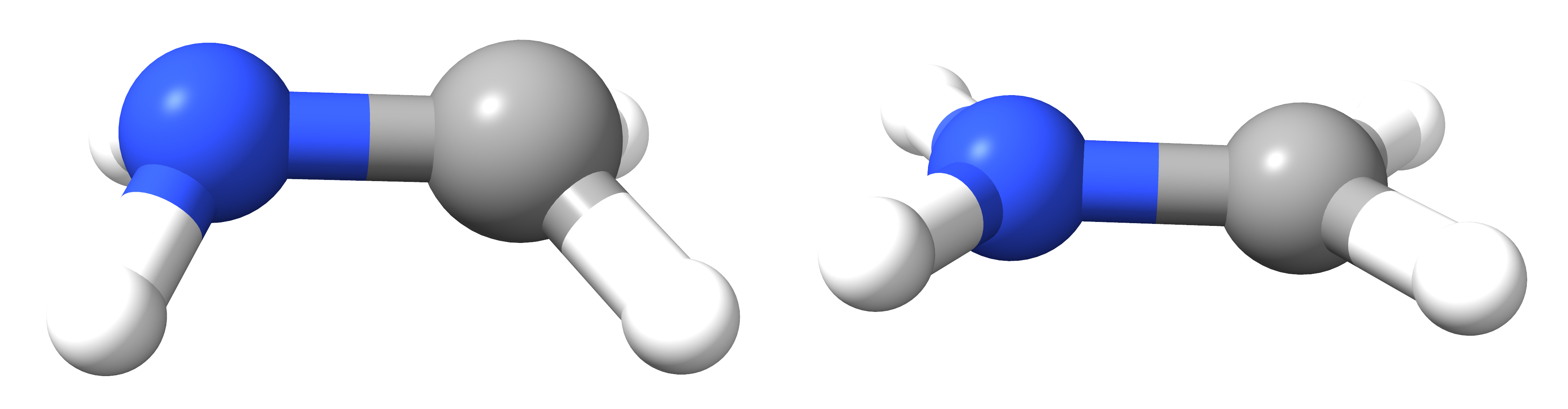
Figure 1: Formaldimine $S_{1}$/$S_{2}$ MECIs with SCCSD($\mathscr{E}$)/cc-pVTZ, distorted (left) and planar (right).

	CCSD	SCCSD		XMS-CASPT2 [33]	MP2/ADC(2) [33]	TD-DFT [33]
		($\mathscr{E}$)	($\mathscr{K}$)
$S_{0}$ minimum	1.271	-	-	1.281	1.275	1.274
Planar MECI	1.426	1.426	1.426	1.420	1.389	1.541
Distorted MECI	1.433	1.433	1.433	-	-	-

Table 1: C-N bond lengths (in $\mathrm{\SIUnitSymbolAngstrom}$) in protonated formaldimine at the $S_{0}$ minimum and at $S_{2}$/$S_{1}$ minimum energy conical intersections. The TD-DFT calculations (from Ref. 33) use the cc-pVDZ basis set. All other calculations are with the cc-pVTZ basis set.

If we allow the breaking of symmetry (by selecting an initial geometry that is non-planar), we find a distorted MECI with both CCSD and SCCSD that has a slightly longer C-N bond length of $1.433$ Å. In this case, the two states are also close to being of different symmetry since the distorted molecule has an approximate mirror plane.

While these results show good agreement with literature,[33] we also find that the system illustrates some limitations of the method. In particular, because the orthogonality equation is non-linear in $\zeta$, it may have more than one solution. For formaldimine, considering a linear interpolation between the Franck-Condon geometry and the distorted MECI, we see that the solution that is well-behaved in the Franck-Condon region breaks down and is replaced by a different well-behaved solution at the MECI (Supplementary Information S4). This indicates that the SCCSD method should be considered a local correction that should only be applied close to the intersection (which is, of course, the only place where it is needed). We should note that this conclusion is likely system-dependent, however, as no such behavior was observed in the thymine simulation.[22] Nevertheless, the presence of multiple solutions shows that a systematic study is needed to fully understand the limitations and the general applicability of the method.

III.1.2 Thymine

The thymine nucleobase efficiently relaxes back to the ground state after excitation by ultraviolet radiation, a property that has been linked to the resilience of our genetic material to radiative damage.[34] The first step in this non-radiative relaxation is believed to be an ultrafast (sub 100-fs) internal conversion from the bright $\pi\pi^{\ast}$ state ($S_{2}$) to a dark $n\pi^{\ast}$ state ($S_{1}$) through a conical intersection seam between these two states, as suggested by several theoretical and experimental studies.[35, 36, 37, 22]

We also find two MECIs for the nucleobase thymine, one that preserves the planar symmetry of the ground state geometry and one that is distorted and non-planar, see Table 2 and Figure 2. In the $\pi\pi^{\ast}$/$n\pi^{\ast}$ photorelaxation, two bond coordinates are believed to be particularly relevant:[35] the C₄-O₈ and C₅-C₆ bonds (see Figure 2). As the system moves away from the Franck-Condon region, it undergoes a long extension of the C₅-C₆ bond and a slight extension of the C₄-O₈ bond. The determined MECIs fit well with this picture, since the observed bond extensions in the simulated dynamics[22] coincide with the bond extensions from the Franck-Condon point to both the planar and distorted MECIs.

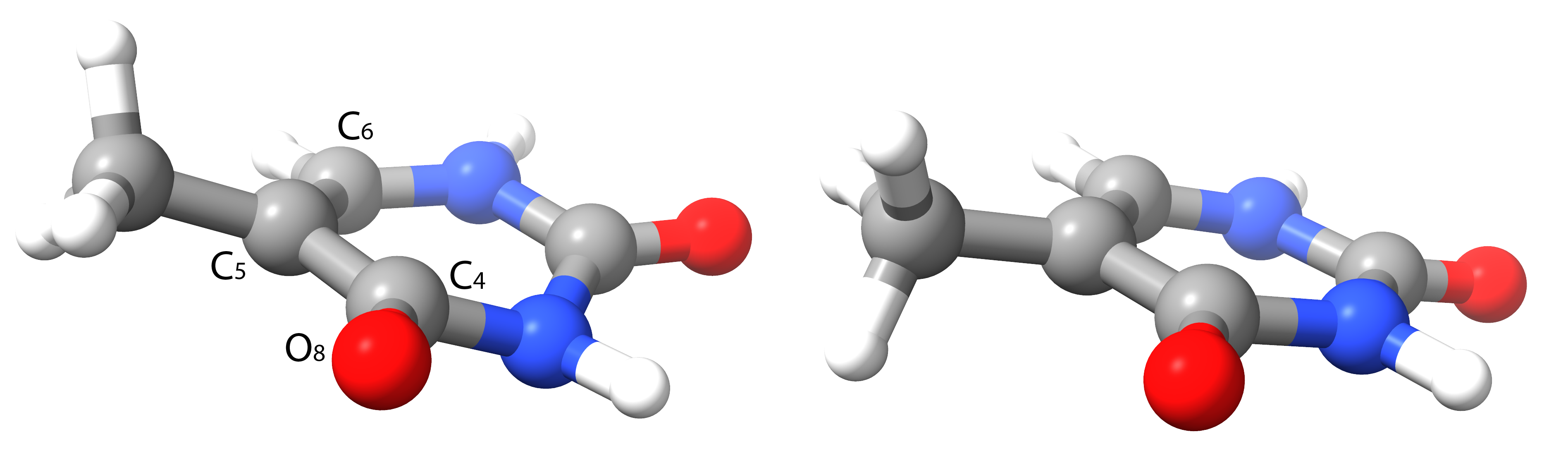
Figure 2: Thymine $S_{1}$/$S_{2}$ MECIs with SCCSD($\mathscr{E}$)/cc-pVDZ, distorted (left) and planar (right). Atomic labels for the C₄-O₈ and C₅-C₆ bonds are shown for the distorted MECI.

	$S_{0}$ minimum	Distorted MECI				Planar MECI
	CCSD	CCSD	SCCSD			CCSD	SCCSD
			($\mathscr{E}$)	($\mathscr{K}$)			($\mathscr{E}$)	($\mathscr{K}$)
C4-O8 (Å)	1.224	1.265*	1.265	1.265		1.251	1.251	1.251
C5-C6 (Å)	1.357	1.446*	1.446	1.446		1.465	1.465	1.465

Table 2: C₄-O₈ and C₅-C₆ bond lengths (in $\mathrm{\SIUnitSymbolAngstrom}$) for thymine at the $S_{2}/S_{1}$ minimum energy conical intersections. The $S_{0}$ minimum was optimized using the aug-cc-pVDZ basis. All other calculations use the cc-pVDZ basis set. The asterisk indicates that the geometry was converged only to within $10^{-3}$ a.u. in the gradient. Other geometries are converged to within $10^{-4}$ a.u.

As for formaldimine, the planar MECIs in thymine are also identical with SCCSD and CCSD, and this is again because $S_{1}$ and $S_{2}$ possess different symmetries. In the non-planar case, we were not able to converge the CCSD MECI due to complex energies encountered during the optimization. Nevertheless, the partially converged MECI coincides with the SCCSD MECI, indicating that the CCSD and SCCSD methods are highly similar in this region of the intersection seam.

III.2 Lithium hydride

As a final illustration, we present derivative coupling elements for lithium hydride. This has been used as a test system of nonadiabatic couplings in CCSD[17, 20] and here we reconsider it for SCCSD. In previous works, the CCSD couplings have been shown to agree well with the full configuration interaction (FCI) couplings, even in the dissociation limit.

In Figure 3, we compare couplings evaluated with standard and similarity constrained coupled cluster methods. Derivative couplings are shown for the $2\,^{1}\Sigma^{+}$/$3\,^{1}\Sigma^{+}$ and $3\,^{1}\Sigma^{+}$/$4\,^{1}\Sigma^{+}$ states, where we consider bond distances near the equilibrium bond length ($2.0$ to $4.4$ bohr). First, we find that the CCSD and SCCSD coupling elements are in close agreement close to the equilibrium (from $2.0$ to $4.0$ bohr), in most cases being so similar that the difference is invisible in the curves in the figure. However, the SCCSD coupling elements break down as the bond is extended beyond $4.0$ bohr for the $3\,^{1}\Sigma^{+}$/$4\,^{1}\Sigma^{+}$ case (see Figure 3, right). We furthermore find that this breakdown is accompanied by a change in the well-behaved solution (see Supporting Information S4).

The breakdown in the dissociation limit is perhaps an unsurprising result, given that coupled cluster theory is often unreliable in this limit. Notably, however, the CCSD method correctly reproduces the nonadiabatic couplings both for the $2\,^{1}\Sigma^{+}$/$3\,^{1}\Sigma^{+}$ and the $3\,^{1}\Sigma^{+}$/$4\,^{1}\Sigma^{+}$ states up to bond lengths as large as 8.0 bohr.[17, 20]

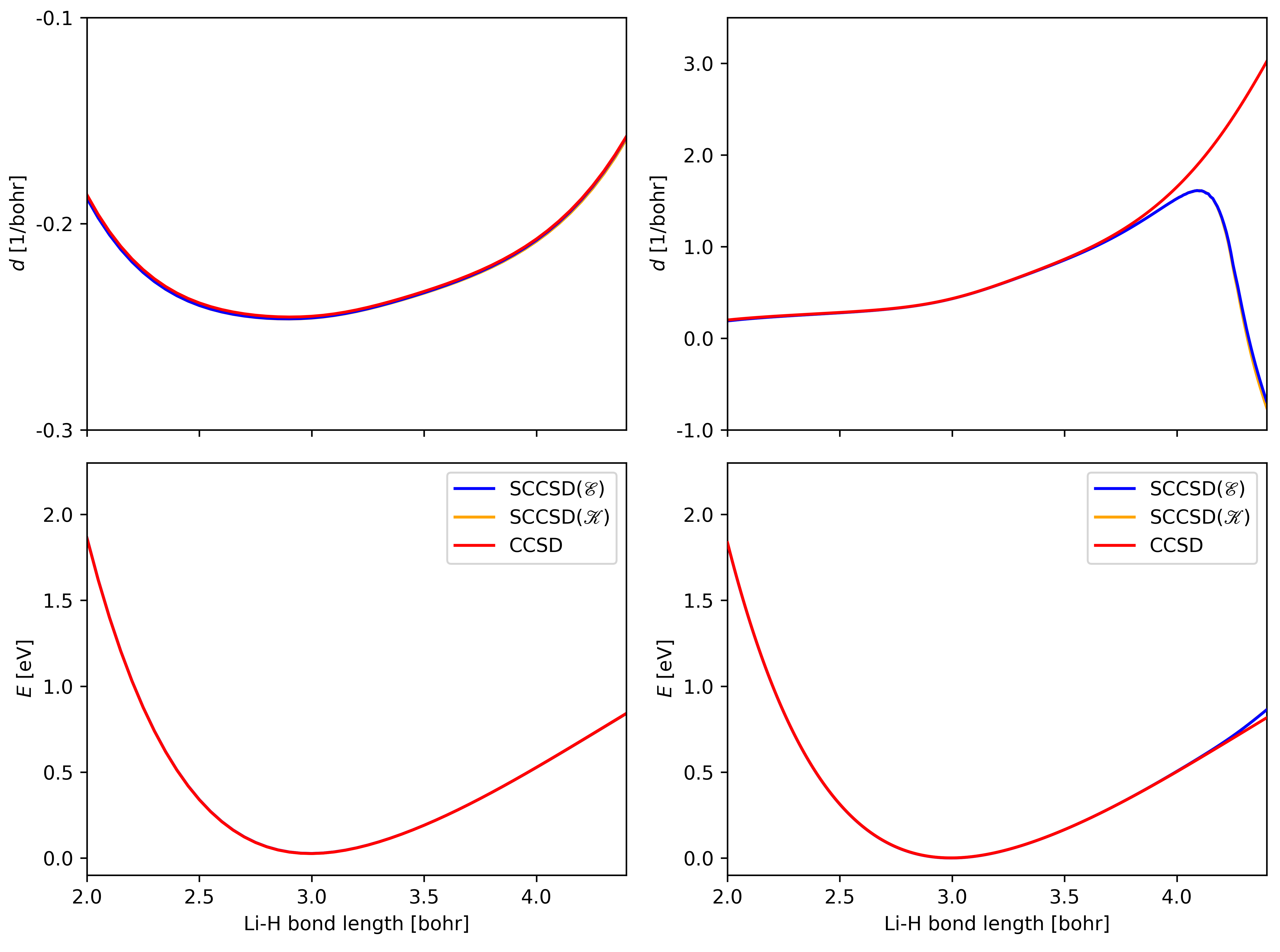
Figure 3: Coupling elements between the $2\,^{1}\Sigma^{+}$/$3\,^{1}\Sigma^{+}$ (top left) and $3\,^{1}\Sigma^{+}$/$4\,^{1}\Sigma^{+}$ (top right) states. The magnitude of the coupling is calculated as $d=2(d_{\mathrm{Li}}-d_{\mathrm{H}})$. Ground state energies are given in the bottom left and right panels. When evaluating the couplings, we have used the normalization described in Ref. 20 on the right coupling elements.

IV Conclusions

In this paper, we have presented an implementation of analytical nuclear gradients and derivative coupling elements for the similarity constrained coupled cluster singles and doubles method (SCCSD), building upon recent implementations for CCSD.[29, 20] We have provided a few numerical examples, showing, for example, good agreement with literature values for a minimum energy conical intersection in protonated formaldimine, a simple model system for the chromophore in rhodopsin. However, we have also shown that the SCCSD method can in some cases have multiple solutions, suggesting that the method must in some cases (though not all, see Ref. 22) be considered a local correction.

Nevertheless, our implementation has made possible the first nonadiabatic dynamics simulations using both CCSD and SCCSD, as demonstrated in a separate nonadiabatic dynamics paper on the ultrafast $\pi\pi^{\ast}$/$n\pi^{\ast}$ photorelaxation in thymine.[22] Given the accurate treatment of dynamical correlation in coupled cluster theory, we expect that its application in nonadiabatic dynamics simulations will provide valuable insights about the photochemistry of a variety of interesting systems.

References

- Domcke, Yarkony, and Köppel [2004] W. Domcke, D. Yarkony, and H. Köppel, Conical intersections: electronic structure, dynamics & spectroscopy, Vol. 15 (World Scientific, 2004).
- Mai and González [2020] S. Mai and L. González, “Molecular photochemistry: recent developments in theory,” Angew. Chem. Int. Ed. 59, 16832–16846 (2020).
- Roos, Taylor, and Sigbahn [1980] B. O. Roos, P. R. Taylor, and P. E. Sigbahn, “A complete active space scf method (casscf) using a density matrix formulated super-ci approach,” Chem. Phys. 48, 157–173 (1980).
- Huix-Rotllant, Ferré, and Barbatti [2020] M. Huix-Rotllant, N. Ferré, and M. Barbatti, “Time-dependent density functional theory,” in Quantum Chemistry and Dynamics of Excited States (John Wiley & Sons, Ltd, 2020) Chap. 2, pp. 13–46.
- Koch and Jørgensen [1990] H. Koch and P. Jørgensen, “Coupled cluster response functions,” J. Chem. Phys. 93, 3333–3344 (1990).
- Stanton and Bartlett [1993] J. F. Stanton and R. J. Bartlett, “The equation of motion coupled-cluster method. a systematic biorthogonal approach to molecular excitation energies, transition probabilities, and excited state properties,” J. Chem. Phys. 98, 7029–7039 (1993).
- Loos et al. [2020] P.-F. Loos, F. Lipparini, M. Boggio-Pasqua, A. Scemama, and D. Jacquemin, “A mountaineering strategy to excited states: Highly accurate energies and benchmarks for medium sized molecules,” J. Chem. Theory Comput. 16, 1711–1741 (2020).
- Hättig [2005] C. Hättig, “Structure optimizations for excited states with correlated second-order methods: CC2 and ADC(2),” Advances in quantum chemistry 50, 37–60 (2005).
- Köhn and Tajti [2007] A. Köhn and A. Tajti, “Can coupled-cluster theory treat conical intersections?” J. Chem. Phys. 127 (2007).
- Kjønstad et al. [2017] E. F. Kjønstad, R. H. Myhre, T. J. Martínez, and H. Koch, “Crossing conditions in coupled cluster theory,” J. Chem. Phys. 147, 164105 (2017).
- Kjønstad and Koch [2017] E. F. Kjønstad and H. Koch, “Resolving the notorious case of conical intersections for coupled cluster dynamics,” The Journal of Physical Chemistry Letters 8, 4801–4807 (2017).
- Kjønstad and Koch [2019] E. F. Kjønstad and H. Koch, “An orbital invariant similarity constrained coupled cluster model,” J. Chem. Theory Comput. 15, 5386–5397 (2019).
- Handy and Schaefer III [1984] N. C. Handy and H. F. Schaefer III, “On the evaluation of analytic energy derivatives for correlated wave functions,” J. Chem. Phys. 81, 5031–5033 (1984).
- Helgaker and Jørgensen [1988] T. Helgaker and P. Jørgensen, “Analytical calculation of geometrical derivatives in molecular electronic structure theory,” Advances in quantum chemistry 19, 183–245 (1988).
- Koch et al. [1990] H. Koch, H. J. A. Jensen, P. Jørgensen, T. Helgaker, G. E. Scuseria, and I. Schaefer, Henry F., “Coupled cluster energy derivatives. Analytic Hessian for the closed‐shell coupled cluster singles and doubles wave function: Theory and applications,” J. Chem. Phys. 92, 4924–4940 (1990).
- Stanton and Gauss [1994] J. F. Stanton and J. Gauss, “Analytic energy gradients for the equation‐of‐motion coupled‐cluster method: Implementation and application to the HCN/HNC system,” J. Chem. Phys. 100, 4695–4698 (1994).
- Tajti and Szalay [2009] A. Tajti and P. G. Szalay, “Analytic evaluation of the nonadiabatic coupling vector between excited states using equation-of-motion coupled-cluster theory,” J. Chem. Phys. 131, 124104 (2009).
- Faraji, Matsika, and Krylov [2018] S. Faraji, S. Matsika, and A. I. Krylov, “Calculations of non-adiabatic couplings within equation-of-motion coupled-cluster framework: Theory, implementation, and validation against multi-reference methods,” J. Chem. Phys. 148 (2018).
- Christiansen [1999] O. Christiansen, “First-order nonadiabatic coupling matrix elements using coupled cluster methods. I. Theory,” J. Chem. Phys. 110, 711–723 (1999).
- Kjønstad and Koch [2023] E. F. Kjønstad and H. Koch, “Communication: Non-adiabatic derivative coupling elements for the coupled cluster singles and doubles model,” J. Chem. Phys. 158, 161106 (2023).
- Schnack-Petersen et al. [2022a] A. K. Schnack-Petersen, H. Koch, S. Coriani, and E. F. Kjønstad, “Efficient implementation of molecular CCSD gradients with Cholesky-decomposed electron repulsion integrals,” J. Chem. Phys. 156, 244111 (2022a).
- Kjønstad et al. [2024] E. F. Kjønstad, O. J. Fajen, A. C. Paul, S. Angelico, D. Mayer, M. Gühr, T. J. A. Wolf, T. J. Martínez, and H. Koch, “Unexpected hydrogen dissociation in thymine: predictions from a novel coupled cluster theory,” (2024), arXiv:2403.01045 [physics.chem-ph] .
- Coester [1958] F. Coester, “Bound states of a many-particle system,” Nucl. Phys. 7, 421–424 (1958).
- Bartlett and Musiał [2007] R. J. Bartlett and M. Musiał, “Coupled-cluster theory in quantum chemistry,” Reviews of Modern Physics 79, 291 (2007).
- Purvis III and Bartlett [1982] G. D. Purvis III and R. J. Bartlett, “A full coupled-cluster singles and doubles model: The inclusion of disconnected triples,” The Journal of Chemical Physics 76, 1910–1918 (1982).
- Hald et al. [2003] K. Hald, A. Halkier, P. Jørgensen, S. Coriani, C. Hättig, and T. Helgaker, “A lagrangian, integral-density direct formulation and implementation of the analytic CCSD and CCSD(T) gradients,” J. Chem. Phys. 118, 2985–2998 (2003).
- Helgaker, Jorgensen, and Olsen [2013] T. Helgaker, P. Jorgensen, and J. Olsen, Molecular electronic-structure theory (John Wiley & Sons, 2013).
- Hohenstein [2016] E. G. Hohenstein, “Analytic formulation of derivative coupling vectors for complete active space configuration interaction wavefunctions with floating occupation molecular orbitals,” J. Chem. Phys. 145 (2016).
- Schnack-Petersen et al. [2022b] A. K. Schnack-Petersen, H. Koch, S. Coriani, and E. F. Kjønstad, “Efficient implementation of molecular CCSD gradients with Cholesky-decomposed electron repulsion integrals,” J. Chem. Phys. 156, 244111 (2022b).
- Folkestad et al. [2020] S. D. Folkestad, E. F. Kjønstad, R. H. Myhre, J. H. Andersen, A. Balbi, S. Coriani, T. Giovannini, L. Goletto, T. S. Haugland, A. Hutcheson, et al., “et 1.0: An open source electronic structure program with emphasis on coupled cluster and multilevel methods,” J. Chem. Phys. 152 (2020).
- Bearpark, Robb, and Bernhard Schlegel [1994] M. J. Bearpark, M. A. Robb, and H. Bernhard Schlegel, “A direct method for the location of the lowest energy point on a potential surface crossing,” Chem. Phys. Letters 223, 269–274 (1994).
- Aquino, Barbatti, and Lischka [2006] A. J. A. Aquino, M. Barbatti, and H. Lischka, “Excited-state properties and environmental effects for protonated schiff bases: A theoretical study,” ChemPhysChem 7, 2089–2096 (2006).
- Taylor, Tozer, and Curchod [2023] J. T. Taylor, D. J. Tozer, and B. F. E. Curchod, “On the description of conical intersections between excited electronic states with LR-TDDFT and ADC(2),” J. Chem. Phys. 159, 214115 (2023).
- Crespo-Hernandez et al. [2004] C. E. Crespo-Hernandez, B. Cohen, P. M. Hare, and B. Kohler, “Ultrafast excited-state dynamics in nucleic acid,” Chem. Rev. 104, 1977–2020 (2004).
- Wolf et al. [2017] T. Wolf, R. H. Myhre, J. Cryan, S. Coriani, R. Squibb, A. Battistoni, N. Berrah, C. Bostedt, P. Bucksbaum, G. Coslovich, et al., “Probing ultrafast */n* internal conversion in organic chromophores via K-edge resonant absorption,” Nat. Commun. 8, 29 (2017).
- Wolf and Gühr [2019] T. J. A. Wolf and M. Gühr, “Photochemical pathways in nucleobases measured with an X-ray FEL,” Philos. Trans. R. Soc. A 377, 20170473 (2019).
- Mayer, Lever, and Gühr [2024] D. Mayer, F. Lever, and M. Gühr, “Time-resolved x-ray spectroscopy of nucleobases and their thionated analogs,” J. Photochem. Photobiol. (2024).