Policy Optimization for PDE Control with a Warm Start

Abstract

Dimensionality reduction is crucial for controlling nonlinear partial differential equations (PDE) through a “reduce-then-design” strategy, which identifies a reduced-order model and then implements model-based control solutions. However, inaccuracies in the reduced-order modeling can substantially degrade controller performance, especially in PDEs with chaotic behavior. To address this issue, we augment the reduce-then-design procedure with a policy optimization (PO) step. The PO step fine-tunes the model-based controller to compensate for the modeling error from dimensionality reduction. This augmentation shifts the overall strategy into reduce-then-design-then-adapt, where the model-based controller serves as a warm start for PO. Specifically, we study the state-feedback tracking control of PDEs that aims to align the PDE state with a specific constant target subject to a linear-quadratic cost. Through extensive experiments, we show that a few iterations of PO can significantly improve the model-based controller performance. Our approach offers a cost-effective alternative to PDE control using end-to-end reinforcement learning.

1 Introduction

Closed-loop control of spatio-temporal systems such as turbulent flows promises enhanced energy efficiency in various applications, including vehicle dynamics, chemical and combustion processes, and heating, ventilation, and air conditioning (HVAC) systems [1]. The primary challenges of controlling such systems are the strong nonlinearity and the infinite dimensionality of the governing nonlinear partial differential equations (PDEs). As a result, computationally permissible control strategies typically involve discretization and dimensionality reduction, followed by applying standard model-based control solutions. This process is known as the reduce-then-design approach [2, 3, 4, 5, 6]. To date, numerous research efforts have focused on developing more accurate reduced-order models (ROMs) for various PDEs [7, 8, 9, 10, 11, 12], thus refining the “reduce” part of the two-step process. Although more precise ROMs certainly improve control performance, their increased complexity and nonlinearity can diminish the computational benefits.

In contrast, we focus here on enhancing the “design” part of the process given a coarse ROM. Existing model-based controllers often come with optimality guarantees contingent on the specific dynamical models they are based on [13, 14, 15, 16, 17]. However, the potentially large inaccuracies from reduced-order modeling, as to trade off computational efficiency, can drastically impair control performance, especially in PDEs that model chaotic systems such as turbulent flows. To address this issue, we augment the reduce-then-design procedure with a model-free policy optimization (PO) step that fine-tunes the model-based control gains to compensate for the coarse modeling. This shifts the overall control strategy into reduce-then-design-then-adapt, where the model-based control gains serve as a warm start for model-free PO.

Specifically, we study the state-feedback tracking control problem that aims to align the PDE state with a specific constant target subject to an infinite-horizon linear-quadratic (LQ) cost. First, we discretize the PDE in space and time at a set of grid points to arrive at a finite but high-dimensional nonlinear system. Then, we apply the off-the-shelf Dynamic Mode Decomposition with control (DMDc) [18] to compute a linear surrogate model that reduces the state dimension by at least tenfold. Lastly, we compute the model-based LQ tracking controller and apply it as a warm start for model-free PO. The PO step further fine-tunes the controller gains using nonlinear high-dimensional PDE solutions until convergence.

We demonstrate the effectiveness of the additional PO step through extensive experiments on three nonlinear PDE control tasks governed by Burgers’, Allen-Cahn, and Korteweg-de Vries equations, respectively. With a thirty-two-fold dimensionality reduction in modeling, model-free PO reduces the cost of the model-based LQ tracking controller by $28.0\%$, $15.8\%$, and $36.4\%$, respectively, after only a few iterations. Furthermore, we show that the warm start significantly accelerates the PO process and leads to a more stable training process toward convergence. Our proposed strategy offers a cost-effective solution to PDE control that combines the strengths of model-based and data-driven approaches. It optimizes the reduce-then-design process in applications where fine-grained modeling is impractical. As a by-product, the concept of a computationally cheap warm start could also be beneficial in applying end-to-end reinforcement learning (RL) to PDE control.

1-A Related Literature

Most PDEs produce solutions that reside on a manifold of moderate dimension in the phase space [19]. ROMs take advantage of this property by discovering an approximation of this manifold and a dynamical model within [20, 21]. Decades of research have resulted in numerous data-driven techniques to construct linear and nonlinear ROMs [22, 23, 24]. We employ DMDc due to its offline nature, ability to model the control mapping, and that the generated linear surrogate model enables closed-form computations of optimal controllers. Our proposed strategy generalizes to more complex ROMs, controller parametrizations, and PO schemes.

Our work bridges model-based and data-driven approaches for closed-loop PDE control. Traditionally, ROM-based controllers have been proposed following the reduce-then-design approach [25, 26, 27], but their control performance has been limited by the accuracy of the ROM. To overcome this limitation, a recent trend is to directly learn controllers from data, assuming access to a simulator of the real system. These approaches include genetic algorithms [28], Bayesian optimization [29], and deep RL [30, 31], but they require formidable computational or experimental resources.

Lastly, our work is relevant to the literature on PO for control [32, 33, 34, 35, 36] and the theoretical foundation underlying this approach [37, 38, 39, 40, 41, 42, 43, 44, 45]. In particular, [39] studied the convergence of PO in linear systems with a “small” nonlinear perturbation, where the linear dynamics were utilized to warm start PO for adapting to the nonlinear perturbation. In contrast to [39], we study general nonlinear PDEs where an explicit linear component is not readily identifiable. We propose the generic strategy of first designing a ROM-based controller and then using data-driven PO for fine-tuning.

2 Problem Formulation

We consider one-dimensional PDE control problems with periodic boundary conditions and spatially distributed controls, following the definitions in Section 2.2 of [36]. The spatial domain is defined as $\Omega=[0,L]\subset\mathbb{R}$, where $L$ is its length, and $u(x,t):\Omega\times\mathbb{R}^{+}\rightarrow\mathbb{R}$ represents a continuous field over spatial and temporal coordinates $x$ and $t$, respectively. The PDE dynamics is described by:

$$\frac{\partial u}{\partial t}-\mathcal{F}\left(\frac{\partial u}{\partial x},\frac{\partial^{2}u}{\partial x^{2}},\dots\right)=a(x,t),$$ (2.1)

with $\mathcal{F}$ being a nonlinear differential operator involving spatial derivatives of various orders and depending on various physical parameters, and $a$ representing a distributed control as $a(x,t)=\sum_{j=0}^{n_{a}-1}\Phi_{j}(x)a_{j}(t)$. Here, $a(x,t)$ integrates $n_{a}$ scalar inputs $a_{j}(t)$, each modulated by its forcing support function $\Phi_{j}(x)$, to model energy addition or external influences on the PDE dynamics. The periodic boundary conditions enforce the continuity of $u$ and its spatial derivatives at the boundary of $\Omega$. We use $u_{r}(x)$ to denote the constant target state with which we aim to align the field $u(x,t)$.

We discretize (2.1) in space and time, defining the high- dimensional state $z_{k}\in\mathbb{R}^{n_{z}}$ to represent $u$ at $n_{z}$ equally-spaced points in $\Omega$ at discrete time $k\in\mathbb{N}$, with $t=k\,\Delta t$ and $\Delta t\in\mathbb{R}^{+}$ as the user-defined sampling time. We treat scalar control inputs $a_{i}(t)$ as piecewise constant over each time step $\Delta t$. The PDE dynamics are then approximated by

$$z_{k+1}=f(z_{k},a_{k}),$$ (2.2)

where $f:\mathbb{R}^{n_{z}}\times\mathbb{R}^{n_{a}}\to\mathbb{R}^{n_{z}}$ is a time-invariant function contingent on the physical parameters and forcing support functions $\Phi_{i}$ of the specific PDE, and the initial condition $z_{0}$ is sampled from a distribution $\mathcal{D}$.

2-A State-Feedback Tracking Control

Our objective is to design a state-feedback controller that enables asymptotic tracking of the discretized constant target state $z_{r}\in\mathbb{R}^{n_{z}}$. Specifically, we aim to minimize the LQ tracking cost defined as

$$\hskip 16.00008ptJ:=\mathbb{E}_{z_{0}}\bigg{\{}\sum_{k=0}^{\infty}(z_{k}-z_{r})^{\top}Q(z_{k}-z_{r})+a_{k}^{\top}Ra_{k}\bigg{\}}$$ (2.3)

$$\text{s.t.}\ z_{k+1}=f(z_{k},a_{k}),\ a_{k}=\phi(z_{0},\cdots,z_{k},a_{0},\cdots,a_{k-1}),$$

where $Q\geq 0$ and $R>0$ are the symmetric positive (semi)-definite weighting matrices. The control policy $\phi$ maps all available information up to $k$ to the control input $a_{k}$. Setting $z_{r}$ to $0$ simplifies our setting to the LQ regulation task. Due to the nonlinearity of $f$, there are no general closed-form solutions for the optimal $\phi$ that minimizes the cost (2.3).

2-B Reduced-Order Model Identification

To address the computational challenges posed by a high-dimensional state $z_{k}\in\mathbb{R}^{n_{z}}$, we adopt a two-step strategy: first performing a dimensionality reduction and then designing a state-feedback controller using the ROM. Among numerous data-driven methods to construct a ROM [46], we utilize the DMDc algorithm [18] described in Algorithm 1.

DMDc generates a reduced-order linear model $(A,B)$ using $N$ consecutive snapshots from a single trajectory of the nonlinear system (2.2). The dimensionality reduction is defined by an orthogonal mode-spanning matrix $U\in\mathbb{R}^{n_{z}\times n_{s}}$ generated from DMDc such that $z_{k}\approx Us_{k}$, with $s_{k}\in\mathbb{R}^{n_{s}}$ denoting the reduced-order state with dimension $n_{s}\ll n_{z}$. Then, DMDc identifies the best-fit linear ROM described by

$$s_{k+1}=As_{k}+Ba_{k},$$ (2.4)

where $s_{0}$ is the projection of the initial condition $z_{0}$ onto the reduced-order space, given by $s_{0}=U^{\top}z_{0}$.

0:  A single trajectory of (2.2), i.e., $\{z_{0},\cdots,z_{N}\}$ and $\{a_{0},\cdots,a_{N-1}\}$, truncation values $p$ and $n_{s}$.

0:  Reduced-order system matrices $A\in\mathbb{R}^{n_{s}\times n_{s}}$, $B\in\mathbb{R}^{n_{s}\times n_{a}}$, and the projection matrix $U\in\mathbb{R}^{n_{z}\times n_{s}}$.

1:  Construct the data matrix $\Omega=\begin{bmatrix}Z\\ \Upsilon\end{bmatrix}$, where:

$Z=\left[\begin{array}[]{cccc}\rule{0.8pt}{5.16666pt}{}&\rule{0.8pt}{5.16666pt}{}&&\rule{0.8pt}{5.16666pt}{}\\ z_{0}&z_{1}&\ldots&z_{N-1}\\ \rule{0.8pt}{5.16666pt}{}&\rule{0.8pt}{5.16666pt}{}&&\rule{0.8pt}{5.16666pt}{}\end{array}\right]$,  $Z^{\prime}=\left[\begin{array}[]{cccc}\rule{0.8pt}{5.16666pt}{}&\rule{0.8pt}{5.16666pt}{}&&\rule{0.8pt}{5.16666pt}{}\\ z_{1}&z_{2}&\ldots&z_{N}\\ \rule{0.8pt}{5.16666pt}{}&\rule{0.8pt}{5.16666pt}{}&&\rule{0.8pt}{5.16666pt}{}\end{array}\right]$,  $\Upsilon=\left[\begin{array}[]{cccc}\rule{0.8pt}{5.16666pt}{}&\rule{0.8pt}{5.16666pt}{}&&\rule{0.8pt}{5.16666pt}{}\\ a_{0}&a_{1}&\ldots&a_{N-1}\\ \rule{0.8pt}{5.16666pt}{}&\rule{0.8pt}{5.16666pt}{}&&\rule{0.8pt}{5.16666pt}{}\end{array}\right]$;

2:  Find the $p$-truncated SVD of $\Omega\approx\Psi\Xi\Lambda^{\top}={\footnotesize\begin{bmatrix}\Psi_{Z}\\ \Psi_{\Upsilon}\end{bmatrix}}\Xi\Lambda^{\top}$;

3:  Compute the $n_{s}$-truncated SVD of $Z^{\prime}\approx U\Gamma V^{\top}$;

4:  Generate $A=U^{\top}Z^{\prime}\Lambda\Xi^{-1}\Psi^{\top}_{Z}U$,  $B=U^{\top}Z^{\prime}\Lambda\Xi^{-1}\Psi^{\top}_{\Upsilon}$;

5:  return $A$, $B$, and $U$.

Algorithm 1 DMDc [18]

3 Policy Optimization with a Warm Start

We first formulate the LQ tracking problem based on the ROM (2.4) and present its closed-form solution. Specifically, the tracking objective is defined as

$$\hskip 20.00003ptJ_{R}:=\mathbb{E}_{s_{0}}\bigg{\{}\sum_{k=0}^{\infty}(s_{k}-s_{r})^{\top}\widetilde{Q}(s_{k}-s_{r})+a_{k}^{\top}Ra_{k}\bigg{\}}$$ (3.1)

$$\text{s.t.}\quad s_{r}=U^{\top}z_{r},\ \widetilde{Q}:=U^{\top}QU\geq 0,\ s_{k+1}=As_{k}+Ba_{k},$$

$$\hskip 22.0pta_{k}=\varphi(s_{0},\cdots,s_{k},a_{0},\cdots,a_{k-1}).$$

The linearity and the low dimensionality of the ROM enable the closed-form computation of the $J_{R}$-minimizing control policy $\varphi$. Then, it is natural to apply $\varphi$ back to addressing the original high-dimensional problem (2.3). This could be done by projecting $\{z_{k}\}_{k\geq 0}$ onto the reduced-order space $\mathbb{R}^{n_{s}}$ and using the policy $a_{k}=\varphi(U^{\top}z_{0},\cdots,U^{\top}z_{k},a_{0},\cdots,a_{k-1})$ to generate control inputs. However, dimensionality reduction may introduce significant modeling errors (e.g., when the reduced state dimension $n_{s}$ is too low or the PDE dynamics are highly nonlinear), which limit the performance of $J_{R}$-minimizing control policy $\varphi$ when applied to (2.3). Nonetheless, $\varphi$ provides a valuable, computationally cheap starting point for further policy fine-tuning using trajectories from the nonlinear high-dimensional system (2.2). The structure of this section is as follows: Section 3-A describes the model-based solution to the reduced-order LQ tracking problem (3.1), which serves as a warm start to the PO algorithm in Section 3-B for further fine-tuning.

3-A Model-Based LQ Tracking Controller

For the reduced-order LQ tracking problem (3.1), the optimal controller has the form of [14]:

$$a_{k} =-(R+B^{\top}PB)^{-1}B^{\top}PAs_{k}+(R+B^{\top}PB)^{-1}B^{\top}q_{k+1},$$ (3.2)

$$q_{k} =(A-B(R+B^{\top}PB)^{-1}B^{\top}PA)^{\top}q_{k+1}+\widetilde{Q}s_{r},\quad q_{\infty}=\widetilde{Q}s_{r},$$

where $P$ is the solution of the algebraic Riccati equation

$$P=A^{\top}PA-A^{\top}PB(R+B^{\top}PB)^{-1}B^{\top}PA+\widetilde{Q},\ \widetilde{Q}=U^{\top}QU.$$

Moreover, the closed-loop matrix $A-B(R+B^{\top}PB)^{-1}B^{\top}PA$ has a spectral radius less than $1$. Note that for any square matrix $X$ with a spectral radius less than $1$, it holds that $\sum_{k=0}^{\infty}X^{k}=(I-X)^{-1}$. Therefore, we can rewrite (3.2) as $a_{k}=K^{MB}_{a}s_{k}+K^{MB}_{b}s_{r}$, where $K^{MB}_{a},K^{MB}_{b}$ are the optimal gain matrices independent of the state $s_{k}$ and the target $s_{r}$:

$$K^{MB}_{a} =-(R+B^{\top}PB)^{-1}B^{\top}PA,$$ (3.3)

$$K^{MB}_{b} =(R+B^{\top}PB)^{-1}B^{\top}(I-(A+BK_{a}^{MB})^{\top})^{-1}\widetilde{Q}.$$ (3.4)

A direct application of the $K^{MB}_{a},K^{MB}_{b}$ to the high-dimensional problem (2.3) results in the controller

$$a_{k}=K^{MB}_{a}(U^{\top}z_{k})+K^{MB}_{b}(U^{\top}z_{r}).$$ (3.5)

When the DMDc model is accurate such that the modeling gap is sufficiently small to be negligible, then (3.5) is a good candidate for addressing the original problem (2.3), providing desired performance at very low computational cost. However, in the presence of a large modeling gap, the performance of (3.5) could degrade substantially, which motivates further fine-tuning using PO.

3-B Policy Optimization with a Warm Start

We propose to fine-tune $K^{MB}_{a},K^{MB}_{b}$ using PO to achieve a good balance between performance and computational efficiency, utilizing simulated trajectories of the nonlinear system (2.2) until reaching a (local) minima of (2.3). Specifically, we define the PO problem with respect to the concatenated control policy $\pi:=[K_{a}\ K_{b}]\in\mathbb{R}^{n_{a}\times(2n_{s})}$ as

$$\min_{\pi}\ J(\pi)\quad\text{s.t.}\quad z_{k+1}=f(z_{k},a_{k}),~{}a_{k}=\pi\begin{bmatrix}U^{\top}z_{k}\\ U^{\top}z_{r}\end{bmatrix},$$ (3.6)

where the objective function $J(\pi)$ follows (2.3).

To address (3.6), we employ a derivative-free policy gradient (PG) method utilizing a (two-point) zeroth-order oracle [47, 48, 49]. We define the vanilla PG update rule as

$$\pi_{i+1}=\pi_{i}-\eta\cdot\nabla_{\pi_{i}}J(\pi_{i}),\quad\pi_{0}=[K_{a}^{MB}\ K_{b}^{MB}],$$ (3.7)

where $\eta>0$ is the learning rate and $\nabla_{\pi_{i}}J(\pi_{i})$ is the noisy PG sampled from Algorithm 2.

Upon converging to a local minimum of (2.3), the fine-tuned policy $\pi$ and the dimensionality reduction matrix $U$ are applied in tandem to address the high-dimensional control problem defined in (2.3). The effectiveness and efficiency of the proposed framework will be showcased through extensive numerical experiments in the following section.

0:  Policy $\pi$, smoothing radius $r$.

0:  The approximated PG $\nabla_{\pi}J(\pi)$.

1:  Sample a random matrix $\Theta\in\mathbb{R}^{n_{a}\times(2n_{s})}$ from a zero-mean Gaussian distribution, and normalize it to $\|\Theta\|_{F}=1$ ;

2:  Perform symmetric perturbation to $\pi$ by setting $\pi^{+}=\pi+r\cdot\Theta$ and $\pi^{-}=\pi-r\cdot\Theta$ ;

3:  Sample $z_{0}\sim\mathcal{D}$ and perform two rollouts with policy $\pi^{+}$ and $\pi^{-}$, respectively. Collect instantiations of the objective value $J(\pi^{+})$ and $J(\pi^{-})$;

4:  return $\nabla_{\pi}J(\pi)=\frac{n_{a}n_{s}}{r}[J(\pi^{+})-J(\pi^{-})]\Theta$;

Algorithm 2 Zeroth-Order Gradient Oracle

4 Experimental Results

In this section, we present numerical experiments on three nonlinear PDE control problems in the controlgym library [36] that are, respectively, governed by the Burgers’, Allen-Cahn, and Korteweg-de Vries equations. We introduce the setups of these environments below.

(P1): Burgers’ Equation is a nonlinear PDE that models shock formation in water waves and gas dynamics. The temporal dynamics of the velocity $u(x,t)$ is

$$\frac{\partial u}{\partial t}+u\frac{\partial u}{\partial x}-\nu\frac{\partial^{2}u}{\partial x^{2}}=a(x,t),$$

where $\nu>0$ denotes the viscosity coefficient, and the source term $a(x,t)$ is defined according to the forcing functions detailed in Section 2.2 of [36]. In the experiments, we set $\nu=10^{-4}$, the sampling time to $\Delta t=0.05$, the integration time of controlgym’s internal PDE solver to $dt=0.01$, the initial field to $u(x,t=0)=\alpha\cdot\mathrm{sech}(\frac{1}{\beta}(x-\frac{L}{2})$ with $\alpha\sim\texttt{uniform}(0.9,1.1)$ and $\beta\sim\texttt{uniform}(0.04,0.06)$, and $L=1$. The target field is set to $u_{r}(x)=0.1\cdot\cos(2\pi x/L)$.

We also set the problem time horizon to $300$, the number of states to $n_{z}=128$, the number of actions to $n_{a}=6$, the width of each distributed forcing support function to $0.15L$ (cf., [36]), and the weighting matrices to $Q=R=I$. In DMDc, we set $p=8$, $n_{s}=4$, and use $a_{k}\sim\mathcal{N}(0,0.1\cdot I)$ to generate the exploratory system trajectory.

(P2): Allen-Cahn Equation is a nonlinear PDE in materials science that models phase separation in binary alloy systems. The temporal dynamics of $u(x,t)$ in one spatial dimension, with $u=\pm 1$ indicating different phases, is described by

$$\frac{\partial u}{\partial t}-\nu^{2}\frac{\partial^{2}u}{\partial x^{2}}+V(u^{3}-u)=a(x,t),$$

where $\nu>0$ is the diffusivity constant and $V$ is the potential constant. In the experiments, we set $\nu=5\times 10^{-2}$, $V=5$, the sampling and integration times to $\Delta t=dt=0.01$, the initial field to $u(x,t=0)=\alpha+(x-\frac{L}{2})^{2}\cdot\cos(\frac{2\pi}{L}(x-\frac{L}{2}))$ with $\alpha\sim\texttt{uniform}(-0.1,0.1)$, and $L=2$. The target field is set to $u_{r}(x)=-\cos(2\pi x/L)$.

We also choose the problem time horizon to be $80$, the number of states to $n_{z}=256$, the number of actions to $n_{a}=12$, the width of each distributed forcing support function to $0.05L$, and the weighting matrices to $Q=I$ and $R=0.1\cdot I$. In DMDc, we set $p=16$, $n_{x}=8$, and use $u_{t}\sim\mathcal{N}(0,0.1\cdot I)$ to generate the exploratory trajectory.

(P3): Korteweg-de Vries Equation is a nonlinear PDE that models the propagation of solitary waves on shallow water surfaces. The temporal dynamics of $u(x,t)$ is given by

$$\frac{\partial u}{\partial t}+\frac{\partial^{3}u}{\partial x^{3}}-6u\frac{\partial u}{\partial x}=a(x,t).$$

We set the sampling time to $\Delta t=0.01$, the integration time to $dt=0.001$, and the initial field to $u(x,t=0)=-\frac{\alpha}{2}\cdot\mathrm{sech}(\frac{\sqrt{\alpha}}{2}(x-\frac{L}{2}))$ with $\alpha\sim\texttt{uniform}(1,3)$, and $L=20$. The target field is set to $u_{r}(x)=\sin(2\pi x/L)$.

We also choose the problem time horizon to be $200$, the number of states to $n_{z}=256$, the number of actions to $n_{a}=10$, the width of each distributed forcing support function to $0.05L$, and the weighting matrices to $Q=R=I$. In DMDc, we set $p=16$ and $n_{x}=8$, i.e., a 32-fold reduction in the state dimension, and use $u_{t}\sim\mathcal{N}(0,0.01\cdot I)$ to generate the exploratory trajectory.

PO parameters: We choose the learning rates of LQT-PO as $\eta=10^{-4}$ in (P1)-(P2) and $\eta=5\times 10^{-5}$ in (P3). The learning rates of pure PO is $\eta=10^{-5}$ in (P1), $\eta=10^{-4}$ in (P2), and $\eta=5\times 10^{-5}$ in (P3). See Figure 1. The smoothing radius of Algorithm 2 is set to $r=0.1$ in all cases.

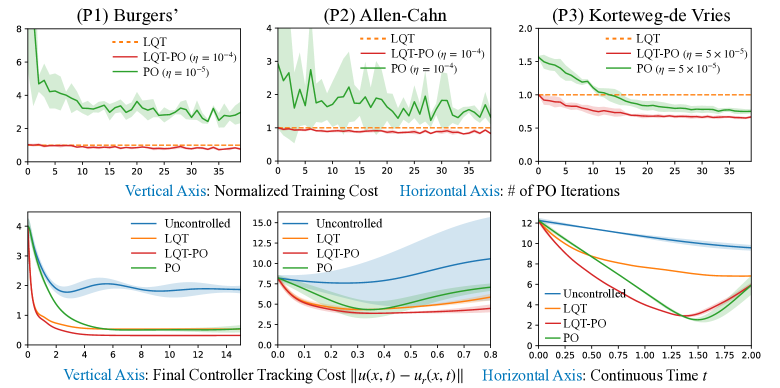
Figure 1: Top: Training curves of model-free PO for (P1)-(P3) averaged over $6$ random seeds with shaded regions denoting standard deviation. We normalize the vertical axis with respect to the cost of the LQT controller based on the DMDc model. For (P1), the training process of PO (without a warm start) instantly destabilizes with $\eta=10^{-4}$. Hence, we select $\eta=10^{-5}$, the largest learning rate under which PO can consistently decrease the cost. Bottom: The tracking costs of (P1)-(P3) with no control, LQT, LQT-PO after 40 iterations, and pure PO after 40 iterations. The costs are averaged over 10 trajectories with randomly sampled initial fields $u(x,t=0)$. The shaded region denotes the standard deviation.

Figure 1 demonstrates that by adding a few iterations of PO, we can reduce the cost of the LQ tracking controller based on DMDc by $28.0\%$, $15.8\%$, and $36.4\%$, respectively, in the three PDE control tasks. Our results confirm the degradation of model-based controllers from the optimum in the presence of a large, unavoidable modeling gap. Consequently, there exist significantly outperforming controllers within the same reduced-order policy space, which could be found using PO. Furthermore, Figure 1 shows that compared to PO from a zero initialization, PO with a (computationally cheap) warm start from the DMDc-based LQ tracking controller exhibits faster and more stable convergence across all three tasks. In the case of (P1), the warm start also allows using a more aggressive learning rate in PO, leading to faster convergence without destabilizing the training process.

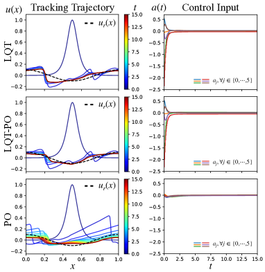
Figure 2: (P1): Comparing model-based, PO with warm start, and pure PO control strategies with $40$ iterations of training budget for the latter two.

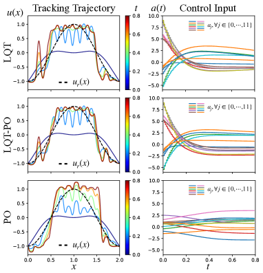
Figure 3: (P2): Comparing model-based, PO with warm start, and pure PO control strategies with $40$ iterations of training budget for the latter two.

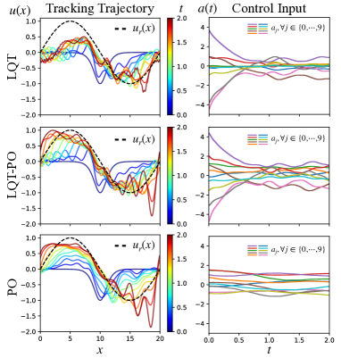
Figure 4: (P3): Comparing model-based, PO with warm start, and pure PO control strategies with $40$ iterations of training budget for the latter two.

In Figures 2, 3, and 4, we compare model-based, PO with warm start, and pure PO control strategies, where the latter two are subject to a certain budget of PO iterations. Each controller’s behavior is evaluated with the initial field $u(x,t=0)$ set to the mean of their respective distributions. The results, as observed across Figures 2-4, indicate that PO with a warm start achieves the best target state tracking among the three control strategies. The numerical results in this section confirm the effectiveness of our methodology.

5 Conclusion

We have augmented the “reduce-then-design” strategy with model-free PO for controlling spatio-temporal systems governed by nonlinear PDEs. Our numerical experiments demonstrate that PO significantly improves the performance of the ROM-based controller against the substantial modeling gap incurred from dimensionality reduction. Conversely, the ROM-based controller facilitates a warm start for PO, leading to accelerated and more stable learning than PO alone. An immediate future research topic is PDE control with imperfect state measurements, necessitating a data-driven state estimator in the controller design [50]. It is also worth considering nonlinear controller parametrizations, possibly through neural networks, and other PO schemes.

References

- [1] Steven L Brunton and Bernd R Noack. Closed-loop turbulence control: Progress and challenges. Applied Mechanics Reviews, 67(5):050801, 2015.
- [2] Jeanne A Atwell, Jeffrey T Borggaard, and B Belinda. Reduced order controllers for Burgers’ equation with a nonlinear observer. International Journal of Applied Mathematics and Computer Science, 11(6):1311–1330, 2001.
- [3] Michael Hinze and Stefan Volkwein. Proper orthogonal decomposition surrogate models for nonlinear dynamical systems: Error estimates and suboptimal control. In Dimension Reduction of Large-Scale Systems: Proceedings of a Workshop held in Oberwolfach, Germany, October 19–25, 2003, pages 261–306. Springer, 2005.
- [4] Friedemann Leibfritz and Stefan Volkwein. Numerical feedback controller design for PDE systems using model reduction: Techniques and case studies. In Real-Time PDE-Constrained Optimization, pages 53–72. SIAM, 2007.
- [5] Svein Hovland, Jan Tommy Gravdahl, and Karen E Willcox. Explicit model predictive control for large-scale systems via model reduction. Journal of guidance, control, and dynamics, 31(4):918–926, 2008.
- [6] Alexandre Barbagallo, Denis Sipp, and Peter J Schmid. Closed-loop control of an open cavity flow using reduced-order models. Journal of Fluid Mechanics, 641:1–50, 2009.
- [7] Sebastian Peitz and Stefan Klus. Koopman operator-based model reduction for switched-system control of PDEs. Automatica, 106:184–191, 2019.
- [8] Kookjin Lee and Kevin T Carlberg. Model reduction of dynamical systems on nonlinear manifolds using deep convolutional autoencoders. Journal of Computational Physics, 404:108973, 2020.
- [9] Kaushik Bhattacharya, Bamdad Hosseini, Nikola B Kovachki, and Andrew M Stuart. Model reduction and neural networks for parametric PDEs. The SMAI Journal of Computational Mathematics, 7:121–157, 2021.
- [10] Stefania Fresca, Luca Dede’, and Andrea Manzoni. A comprehensive deep learning-based approach to reduced order modeling of nonlinear time-dependent parametrized PDEs. Journal of Scientific Computing, 87:1–36, 2021.
- [11] Shady E Ahmed, Suraj Pawar, Omer San, Adil Rasheed, Traian Iliescu, and Bernd R Noack. On closures for reduced order models—a spectrum of first-principle to machine-learned avenues. Physics of Fluids, 33(9), 2021.
- [12] Eurika Kaiser, J Nathan Kutz, and Steven L Brunton. Data-driven discovery of Koopman eigenfunctions for control. Machine Learning: Science and Technology, 2(3):035023, 2021.
- [13] Jacques Louis Lions. Optimal Control of Systems Governed by Partial Differential Equations, volume 170. Springer, 1971.
- [14] Brian DO Anderson and John B Moore. Optimal control: linear quadratic methods, 1990.
- [15] Tamer Başar and Pierre Bernhard. H-Infinity Optimal Control and Related Minimax Design Problems: A Dynamic Game Approach. Birkhäuser, Boston, 1995.
- [16] Miroslav Krstic and Andrey Smyshlyaev. Boundary Control of PDEs: A Course on Backstepping Designs. SIAM, 2008.
- [17] John A Burns, Xiaoming He, and Weiwei Hu. Feedback stabilization of a thermal fluid system with mixed boundary control. Computers & Mathematics with Applications, 71(11):2170–2191, 2016.
- [18] Joshua L Proctor, Steven L Brunton, and J Nathan Kutz. Dynamic mode decomposition with control. SIAM Journal on Applied Dynamical Systems, 15(1):142–161, 2016.
- [19] Albert Cohen and Ronald DeVore. Approximation of high-dimensional parametric PDEs. Acta Numerica, 24:1–159, 2015.
- [20] Peter Benner, Serkan Gugercin, and Karen Willcox. A survey of projection-based model reduction methods for parametric dynamical systems. SIAM Review, 57(4):483–531, 2015.
- [21] Clarence W Rowley and Scott TM Dawson. Model reduction for flow analysis and control. Annual Review of Fluid Mechanics, 49:387–417, 2017.
- [22] Philip Holmes, John Lumley, Gahl Berkooz, and Clarence Rowley. Turbulence, Coherent Structures, Dynamical Systems and Symmetry. Cambridge University Press, 2012.
- [23] Steven L Brunton and J Nathan Kutz. Data-Driven Science and Engineering: Machine Learning, Dynamical Systems, and Control. Cambridge University Press, 2022.
- [24] Boris Kramer, Benjamin Peherstorfer, and Karen E Willcox. Learning nonlinear reduced models from data with operator inference. Annual Review of Fluid Mechanics, 56:521–548, 2024.
- [25] Denis Sipp and Peter J Schmid. Linear closed-loop control of fluid instabilities and noise-induced perturbations: A review of approaches and tools. Applied Mechanics Reviews, 68(2):020801, 2016.
- [26] Chuanqiang Gao, Weiwei Zhang, Jiaqing Kou, Yilang Liu, and Zhengyin Ye. Active control of transonic buffet flow. Journal of Fluid Mechanics, 824:312–351, 2017.
- [27] Alexandros Tsolovikos, Efstathios Bakolas, Saikishan Suryanarayanan, and David Goldstein. Estimation and control of fluid flows using sparsity-promoting dynamic mode decomposition. IEEE Control Systems Letters, 5(4):1145–1150, 2020.
- [28] Thomas Duriez, Steven L Brunton, and Bernd R Noack. Machine Learning Control-Taming Nonlinear Dynamics and Turbulence, volume 116. Springer, 2017.
- [29] Antoine B Blanchard, Guy Y Cornejo Maceda, Dewei Fan, Yiqing Li, Yu Zhou, Bernd R Noack, and Themistoklis P Sapsis. Bayesian optimization for active flow control. Acta Mechanica Sinica, pages 1–13, 2021.
- [30] Dixia Fan, Liu Yang, Zhicheng Wang, Michael S Triantafyllou, and George Em Karniadakis. Reinforcement learning for bluff body active flow control in experiments and simulations. Proceedings of the National Academy of Sciences, 117(42):26091–26098, 2020.
- [31] Paul Garnier, Jonathan Viquerat, Jean Rabault, Aurélien Larcher, Alexander Kuhnle, and Elie Hachem. A review on deep reinforcement learning for fluid mechanics. Computers & Fluids, 225:104973, 2021.
- [32] Draguna Vrabie, O Pastravanu, Murad Abu-Khalaf, and Frank L Lewis. Adaptive optimal control for continuous-time linear systems based on policy iteration. Automatica, 45(2):477–484, 2009.
- [33] John Schulman, Philipp Moritz, Sergey Levine, Michael Jordan, and Pieter Abbeel. High-dimensional continuous control using generalized advantage estimation. arXiv preprint arXiv:1506.02438, 2015.
- [34] Timothy P Lillicrap, Jonathan J Hunt, Alexander Pritzel, Nicolas Heess, Tom Erez, Yuval Tassa, David Silver, and Daan Wierstra. Continuous control with deep reinforcement learning. arXiv preprint arXiv:1509.02971, 2015.
- [35] Benjamin Recht. A tour of reinforcement learning: The view from continuous control. Annual Review of Control, Robotics, and Autonomous Systems, 2:253–279, 2019.
- [36] Xiangyuan Zhang, Weichao Mao, Saviz Mowlavi, Mouhacine Benosman, and Tamer Başar. Controlgym: Large-scale safety-critical control environments for benchmarking reinforcement learning algorithms. arXiv preprint arXiv:2311.18736, 2023.
- [37] Maryam Fazel, Rong Ge, Sham M Kakade, and Mehran Mesbahi. Global convergence of policy gradient methods for the linear quadratic regulator. In International Conference on Machine Learning, pages 1467–1476, 2018.
- [38] Kaiqing Zhang, Bin Hu, and Tamer Başar. Policy optimization for linear control with robustness guarantee: Implicit regularization and global convergence. SIAM Journal on Control and Optimization, 59(6):4081–4109, 2021.
- [39] Guannan Qu, Chenkai Yu, Steven Low, and Adam Wierman. Combining model-based and model-free methods for nonlinear control: A provably convergent policy gradient approach. arXiv preprint arXiv:2006.07476, 2020.
- [40] Kaiqing Zhang, Xiangyuan Zhang, Bin Hu, and Tamer Başar. Derivative-free policy optimization for linear risk-sensitive and robust control design: Implicit regularization and sample complexity. Advances in Neural Information Processing Systems, 34:2949–2964, 2021.
- [41] Xiangyuan Zhang and Tamer Başar. Revisiting LQR control from the perspective of receding-horizon policy gradient. IEEE Control Systems Letters, 7:1664–1669, 2023.
- [42] Xiangyuan Zhang, Bin Hu, and Tamer Başar. Learning the Kalman filter with fine-grained sample complexity. arXiv preprint arXiv:2301.12624, 2023.
- [43] Bin Hu, Kaiqing Zhang, Na Li, Mehran Mesbahi, Maryam Fazel, and Tamer Başar. Toward a theoretical foundation of policy optimization for learning control policies. Annual Review of Control, Robotics, and Autonomous Systems, 6:123–158, 2023.
- [44] Xiangyuan Zhang, Raj Kiriti Velicheti, and Tamer Başar. Learning minimax-optimal terminal state estimators and smoothers. In 22nd IFAC World Congress, pages 12391–12396, 2023.
- [45] Xiangyuan Zhang, Saviz Mowlavi, Mouhacine Benosman, and Tamer Başar. Global convergence of receding-horizon policy search in learning estimator designs. arXiv preprint arXiv:2309.04831, 2023.
- [46] Kunihiko Taira, Steven L Brunton, Scott TM Dawson, Clarence W Rowley, Tim Colonius, Beverley J McKeon, Oliver T Schmidt, Stanislav Gordeyev, Vassilios Theofilis, and Lawrence S Ukeiley. Modal analysis of fluid flows: An overview. AIAA Journal, 55(12):4013–4041, 2017.
- [47] Abraham D Flaxman, Adam Tauman Kalai, and H Brendan McMahan. Online convex optimization in the bandit setting: Gradient descent without a gradient. In ACM-SIAM Symposium on Discrete Algorithms, pages 385–394, 2005.
- [48] John C Duchi, Michael I Jordan, Martin J Wainwright, and Andre Wibisono. Optimal rates for zero-order convex optimization: The power of two function evaluations. IEEE Transactions on Information Theory, 61(5):2788–2806, 2015.
- [49] Yurii Nesterov and Vladimir Spokoiny. Random gradient-free minimization of convex functions. Foundations of Computational Mathematics, 17(2):527–566, 2017.
- [50] Saviz Mowlavi, Mouhacine Benosman, and Saleh Nabi. Reinforcement learning-based estimation for partial differential equations. In SIAM Conference on Applications of Dynamical Systems, 2023.