An exciting hint towards the solution of the neutron lifetime puzzle?

Abstract

We revisit the neutron lifetime puzzle, a discrepancy between beam and bottle measurements of the weak neutron decay. Since both types of measurements are realized at different times after the nuclear production of free neutrons, we argue that the existence of an excited state could be responsible for the different lifetimes. We elaborate on the required properties of such a state and construct a concrete toy model with several of the required characteristics.

I Introduction

I.1 The neutron in the quark model

The neutron is one of the main constituents of nuclear matter. It is a composite state, whose properties are ruled by the strong and the electroweak interactions between the lightest quarks of the Standard Model of particle physics. It is of pivotal importance in many phenomena ranging from Big Bang Nucleosynthesis to experimental particle physics ParticleDataGroup:2022pth

Even though, a detailed understanding of the low energy properties of this particle in terms of fundamental degrees of freedom is an open field of research, it is possible to understand several properties in terms of much simpler models. In our discussion we will make use of the language and notation of the quark model. In this model, protons and neutrons are composite particles made up of quarks. Protons consist of a particular combination two “up” ($u$) quarks and one “down” ($d$) quark, while neutrons consist of combinations of one up quark and two down quarks. Quarks carry a fractional electric charge, and the combination of quarks in protons and neutrons results in particles with integer electric charges.

Isospin describes the similarity between protons and neutrons. It was introduced by Werner Heisenberg and later developed further by Eugene Wigner Heisenberg:1932dw ; Wigner:1936dx . Algebraically, the isospin operator $\vec{I}$, can be represented analogously to the spin operator of spin one half particles $\vec{S}$ in terms of the Pauli matrices $\sim\vec{\sigma}$, which are a representation of the group $SU(2)$. In the quark model it is imposed that both $\vec{I}$ and $\vec{S}$ are (approximate) symmetries. Thus actions of the group memebers are to be understood as symmetry transformations. Based on this, one imposes that the neutron wave function is an eigenfunction of $(\vec{I}^{2},\,I_{z})$ with the eigenvalues $(3/4,\,-1/2)$ while the proton has the eigenvalues $(3/4,+1/2)$. Further imposing that these particles carry spin $\pm 1/2$ like their three constituents singles out a unique state for the neutron (e.g. with spin up $\uparrow$ GreinerMueller )

$$|n\uparrow\rangle=\frac{1}{3\sqrt{2}}\left(|udd\rangle|dud\rangle|ddu\rangle\right)\left(\begin{array}[]{rrr}2&-1&-1\\ -1&2&-1\\ -1&-1&2\end{array}\right)\left(\begin{array}[]{c}|\downarrow\uparrow\uparrow\rangle\\ |\uparrow\downarrow\uparrow\rangle\\ |\uparrow\uparrow\downarrow\rangle\\ \end{array}\right).$$ (1)

The corresponding unique state for the proton is obtained analogously by replacing $u\leftrightarrow d$. If the isospin symmetry were an exact symmetry protons and neutrons would have the same energy and thus the same mass. The observed difference between the neutron mass $m_{n}$ and the proton mass $m_{p}$ and the aforementioned neutron decay show that $I_{z}$ must be broken. In the above description, this breaking is modeled by associating a larger mass to up quarks than to down quarks $m_{u}<m_{d}$. This generates a mass splitting between $|n\uparrow\rangle$ and $p\uparrow\rangle$. Also the conservation of spin is only an approximate concept, due to the presence of gluons, virtual quark antiquark pairs, and the respective angular momenta. Interestingly, the presence of these virtual particles can be effectively absorbed in the concept of constituent quarks as “dressed” color states Lavelle:1995ty which combine such that they form color neutral hadrons. This, and other, more sophisticated models of the neutron, in combination with experimental efforts allowed to learn more and more details about the properties such as mass, composition, and lifetime ParticleDataGroup:2022pth . Thus, it is fair to say that quark models have proven to be useful for our understanding of the internal structure of hadrons Eichmann:2016yit .

Since we will exemplify our ideas with a model which has also three quarks, a word of caution is in place here. There are several phenomenological aspects which can hardly be captured even by our most sophisticated theoretical models, not to speak by simple three-quark models.

• Mass:
  The simple quark model fails when one attempts to predict the precise mass of hadrons GreinerMueller .

• Spin:
  The structure of the spin distribution inside of a neutron wave-function is largely unknown (for a review see Deur:2018roz ). However, there is certain agreement that the valence quarks only carry a fraction of the neutron spin, which was at times labeled as “spin crisis” Veneziano:1989ei ; Anselmino:1988hn ; Nayak:2018nrv .

• Radius:
  The radius of the proton has been deduced from complementary measurements and the resulting $4\%$ disagreement became widely known as the “proton radius puzzle” (for a review see Carlson:2015jba ).

• Neighbors:
  The inner structure of protons and neutrons seems to be strongly sensitive to the neighboring hadrons within a nucleus. This puzzling behaviour is known as EMC effect Geesaman:1995yd .

• Lifetime:
  Last but not least, there is a tension between different measurements of the neutron’s lifetime (see e.g. Paul:2009md ; Serebrov:2011re ).

Thus, any three-quark model should be understood as useful tool for qualitative understanding rather than for precise quantitative modelling.

The last item on the above list will be the subject of interest of this paper. It will therefore be summarized in the following subsection.

I.2 The lifetime puzzle

In this study, we will focus on a discrepancy in the lifetime of the neutron, known as the Neutron Lifetime Puzzle (N$\lambda$P):

Beam neutrons have an about 10 sec longer lifetime than Ultra Cold Neutrons (UCN) in bottle traps  Paul:2009md ; Wietfeldt:2011suo ; Ezhov:2014tna ; Pattie:2017vsj ; Serebrov:2018yxq ; UCNt:2021pcg . The corresponding normalized difference for UCNs in gravitational bottle traps and average beam results is

$$\Delta\tau=\tau_{\mathrm{beam}}-\tau_{\mathrm{bottle}}=(8.6\pm 2.2)\,\mathrm{s}.$$ (2)

One expects this quantity to be compatible with zero and the fact that it is significantly different from zero is known as the N$\lambda$P. This puzzle has persisted over the years, and recently, a possible explanation due to exotic decay channels was excluded Klopf:2019afh ; Dubbers:2018kgh . An alternative theoretical conjecture is based on neutron oscillations Berezhiani:2018eds ; Berezhiani:2018xsx ; Tan:2023mpj ; Altarev:2009tg . Also this possibility has, been largely constrained Broussard:2021eyr . Further, conjectures include Kaluza–Klein states Dvali:2023zww , modifications of the CKM matrix induced at the TeV scale Belfatto:2019swo , and dark photons Barducci:2018rlx . Also concerns about the systematic error in beam experiments have been raised Serebrov:2020rvv , but a contradicting response was given in Wietfeldt:2023nlh . Thus, the status of how to interpret, or understand the N$\lambda$P (2) is still inconclusive. What makes this problem even more interesting is the fact that it is not only a pressing problem for theoretical model building, it is a disagreement between two complementary types of experiments. Clearly, it would be helpful to have more results with beam experiments, but meanwhile we opt to trust the results of our experimental colleagues. Thus, a solution of this discrepancy is urgently needed.

I.3 Structure of the paper

In the following section II we present our working hypothesis and formulate necessary conditions for a solution of the N$\lambda$P in terms of an excited state. In section III we provide a toy model that is able to fulfill most of these necessary conditions. In section IV we explore the parameter space of the toy model and discuss observational issues and known analogies in physics. Conclusions are given in section V.

II Excited states hypothesis

Beam neutrons and UCNs are very similar with respect to most important characteristics. There are, however, some interesting differences. First of all there is the difference in velocity. While neutron beams operate typically with velocity at the order of ${\mathcal{O}}(10^{3}\,\mathrm{m/s})$, neutrons in bottles have velocities of ${\mathcal{O}}(10^{0}\,\mathrm{m/s})$. Another distinction is time. Beam neutrons are measured very shortly after their production in the reactor. The time scale for this is of the order of $t_{\mathrm{beam}}\sim 25ms$. Bottle neutrons, instead, have to undergo a process of slowing, orienting, and cleaning, which means that their weak decay is measured a long time after their production $t_{\mathrm{bottle}}>300\,\mathrm{s}$ UCNt:2021pcg .

This difference is the motivation for our proposal. Let us assume that the neutron wave functions can have excited states, which are not present for neutrons within a strongly bound hadronic ensemble. For example, let us further assume that there is a ground state $\Psi_{g}$ and an excited state $\Psi_{e}$ with corresponding the lifetimes under beta decay of

$$\tau_{g} = 878\,\mathrm{s},$$ (3)

$$\tau_{e}\equiv\tau_{g}+|\Delta\tau_{e}| \geq \tau_{g}+|\Delta\tau|$$

The states neutron states shall be connected by an electromagnetic channel with half-life time $\tau_{\gamma}$

$$\Psi_{e} \rightarrow \Psi_{g}+\gamma.$$ (4)

The characteristic times for the transitions shall be

$$t_{\mathrm{beam}}(\approx 2\times 10^{-2}\,\mathrm{s})\ll\tau_{\gamma}<t_{\mathrm{bottle}}<\tau_{g}(=878\,\mathrm{s})<\tau_{e}(=888\,\mathrm{s}).$$ (5)

Then the change rate of the corresponding particle numbers in these states is

$$\dot{n}_{e} = -n_{e}\left(\frac{1}{\tau_{\gamma}}+\frac{1}{\tau_{e}}\right),$$ (6)

$$\dot{n}_{g} = n_{e}\left(\frac{1}{\tau_{\gamma}}\right)-n_{g}\left(\frac{1}{\tau_{g}}\right).$$

Since the two states $\Psi_{e},\,\Psi_{g}$ are, from the experimental perspective, indistinguishable, both would be counted together

$$n_{n}=n_{g}+n_{e},$$ (7)

and the lifetime would be extracted from

$$\tau_{n}=-\frac{n_{n}}{\dot{n}_{n}}.$$ (8)

This observable is plotted in Figure 1, where we solved the equations (6) numerically for $\tau_{\gamma}=4\,$s and $n_{e}(0)=1,\;n_{g}(0)=0$.

Figure 1: Effective lifetime (8) as a function of the time for an exemplary value of $\tau_{\gamma}=4\,$s.

One sees clearly that such a constellation would offer a potential solution for the lifetime puzzle. Apart from the numerical solution, the time hierarchy (5) also allows to get an analytical understanding of how the two different lifetimes for beam and bottle experiments come about. For this we define

$$\Delta\tau_{e}=\tau_{e}-\tau_{g}.$$ (9)

The lifetime puzzle arises from count rates at two different sites:

• Since $t_{\mathrm{beam}}\ll$ all other times, one can identify the beam abundances as the initial abundances $n_{i}(0)$. Imposing that $\tau_{n}(0)\equiv\tau_{g}+|\Delta\tau|$ and using relation (8) one can solve for the initial relative abundances that mimic this value

  $$\frac{n_{e}(0)}{n_{g}(0)}\approx\frac{\Delta\tau}{\Delta\tau_{e}-\Delta\tau}+{\mathcal{O}}\left(\frac{\Delta\tau}{\tau_{g}}\right)^{2}.$$ (10)

  From this relation one realizes that $\Delta\tau_{e}\geq\Delta\tau$ and that for the extremal case $\Delta\tau_{e}\rightarrow\Delta\tau$ all initial states need to be excited $n_{g}(0)\rightarrow 0$.

• Since, $t_{\mathrm{bottle}}\gg$ “all other time-scales”, all remaining neutrons are in the ground state. Thus,

  $$\tau_{n}(t_{\mathrm{bottle}})=\tau_{g}.$$ (11)

Let us briefly summarize the necessary ingredients that we identified to make the proposal work:

• There is at least one excited state of the free neutron $\Psi_{e}$ above the ground state $\Psi_{g}$.

• The lifetime of the excited state under beta decay is larger than, or equal to, the lifetime of the ground state plus the absolute value of the N$\lambda$P.

• The lifetime for the electromagnetic transition $\Psi_{e}\rightarrow\Psi_{g}$ lies between the time-scales of beam and bottle experiments ($t_{\mathrm{beam}}<\tau_{\gamma}<t_{\mathrm{bottle}}$). This hierarchy (5) of lifetimes is sketched in Figure (2).

  

  Figure 2: a

• The energy difference between $\Psi_{e}$ and $\Psi_{g}$ is smaller than $\sim 10\,$MeV, such that they can be excited with the initial kinetic energy available from nuclear fission.

• When a free neutron is created from a nuclear reaction, the initial abundancy of the excited state is (10).

• The state $\Psi_{e}$ is not populated if the neutron is strongly bound within a nucleus.

As add on to condition c) one should also consider other observables from different experiments. This topic will be touched in section IV. If these conditions are realized, they imply a preferred decay cascade for the initially produced state $\Psi_{e}$. This cascade is indicated by Figure 3.

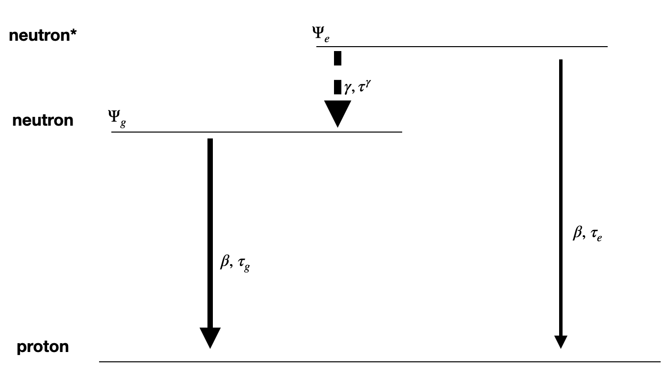
Figure 3: Schematic energy levels of the cascade. The thickness of the arrows indicates the increased probability of certain channels.

The items (a–f) are necessary conditions for an alternative solution of the N$\lambda$P. How could this be realized? Differences in lifetimes under beta decay of states with identical couplings at the quark level can be conceived in two different ways. The first possibility is an enhanced phase space. The decay of an excited state with larger energy has a larger phase space, than the decay of a ground state, which can result in a reduced lifetime. The second possibility are selection rules. If the quantum numbers of the excited state are such that a beta decay is (partially) forbidden or disfavored. While the former option would worsen the N$\lambda$P, the latter option is worth to be explored further. For this, we will recur to a simple toy model, where a neutron is built of three quarks $udd$, which are assumed to carry it’s total spin, while neglecting the contributions of internal angular momentuma and virtual particles.

III A model with three quarks

The purpose of this section is to give an idea of how the above hypothesis can be implemented in terms of a simple but concrete model. Let us assume that a neutron consists of three non-relativistic constituent quarks $udd$. Isospin is an approximate symmetry, which is valid at energies above $4~{}$MeV. Below this energy this symmetry is broken due to the mass splitting between the up and the down quark $m_{u}>m_{d}$. This breaking is, however, only responsible for the explanation of the neutron as an excited state of the proton. It is not sufficient to implement the hypothesis of an excited neutron state far below the Roper resonance (concerning this resonance in the quark model e.g. Eichmann:2016yit ). Since we ware interested in excitations far below the $4~{}$MeV scale, up-quarks and down-quarks are to be considered as different particle species. The neutron is then formed of two representatives of the different particle species which are not (any more) related by a symmetry. In this sense the $udd$ system is analogous to a $He^{3}$ atom, which consists of two lighter fermions with negative charge (electrons corresponding to down quarks) and one doubly charged heavier fermion ($He^{++}$ nucleus corresponding to the up quark). In atomic $He$ the exchange interaction leads to a splitting of energy states with different spin configurations. We will seek for something analogous in the $udd$ system.

There are, however, two important difference which limits the applicability of this analogy between the neutron and $He^{3}$. First, the mass difference between nucleus and electron is by far more pronounced than the difference between up and down quarks. Second, the constituent quarks carry the confining charge of the strong interaction, while the atom is only subject to electromagnetic interactions. One important consequence of this second fact is that the wave function of a neutron in our model depends on colour in addition to the position, and angular momentum quantum numbers. Let’s assume that these contributions factorize as a product $\Psi=\Phi\cdot\Xi\cdot C$ of a spatial part $\Phi(\vec{r}_{d,1},\vec{r}_{d,2},\vec{r}_{u})$, a spin part $\Xi_{\sigma_{d,1},\sigma_{d,2},\sigma_{u}}$ and a color part $C(c_{1},c_{2},c_{3})$, where $\vec{r}_{d,1},\vec{r}_{d,2},\vec{r}_{u}$ and $\sigma_{d,1},\sigma_{d,2},\sigma_{u}$ denote the spatial and the spin coordinates of the $udd$ quarks, respectively, in the restframe of the center of gravity. The total wave function must be anti-symmetric under exchange of any of the quarks. Color confinement requires anti-symmetry in the color quantum numbers and allows the color part of the wave function to be factored out. The remaining spin and spatial part must therefore be symmetric under the exchange of two down quarks

$$\Phi(\vec{r}_{d,1},\vec{r}_{d,2},\vec{r}_{u})\Xi_{\sigma_{d,1},\sigma_{d,2},\sigma_{u}}=\Phi(\vec{r}_{d,2},\vec{r}_{d,1},\vec{r}_{u})\Xi_{\sigma_{d,2},\sigma_{d,1},\sigma_{u}}.$$ (12)

We suppose that the total spin of the neutron is 1/2 in accordance with the measured spin of neutrons at all times. Excited states of the neutron with a total spin $3/2$ are known as delta baryons, but again, these are far heavier than the neutron itself ParticleDataGroup:2022pth .

III.1 Spin wave functions

We start considering the possible spin parts $\Xi$ of the model wave functions of the neutron and later turn to the respective spatial parts. First, the $d$-spins can be combined to a total spin of the $d$-quarks $S_{d}$ and the corresponding $z$-projection $S_{d,z}$. We label the spin states with a quantum number for total spin and a quantum number for the $\hat{z}$ projection $|S_{d},S_{d,z}\rangle_{d}$. There are three symmetric $d$-triplet states

$$|1,+1\rangle_{d} =|\uparrow\uparrow\rangle_{d}, |1,0\rangle_{d} =\frac{1}{\sqrt{2}}\left(|\uparrow\downarrow\rangle_{d}+|\downarrow\uparrow\rangle_{d}\right), |1,-1\rangle_{d} =|\downarrow\downarrow\rangle_{d},$$ (13)

and one anti-symmetric $d$-singlet state

$$|0,0\rangle_{d}=\frac{1}{\sqrt{2}}\left(|\uparrow\downarrow\rangle_{d}-|\downarrow\uparrow\rangle_{d}\right).$$ (14)

There are four linearly independent combinations of these states with the $|\downarrow\rangle_{u},\,|\uparrow\rangle_{u}$ spin states of the $u$-quark that are eigenstate of $\hat{S}^{2}$ with a total spin $S$ of $1/2$. Using the notation $|S,S_{z},S_{d}\rangle$, the two possibilities having $S_{z}=+1/2$ are

$$\Xi_{1}=\left|\frac{1}{2},\frac{1}{2},1\right\rangle = \sqrt{\frac{2}{3}}|1,1\rangle_{d}|\downarrow\rangle_{u}-\frac{1}{\sqrt{3}}|1,0\rangle_{d}|\uparrow\rangle_{u},$$ (15)

$$\Xi_{2}=\left|\frac{1}{2},\frac{1}{2},0\right\rangle = |0,0\rangle_{d}|\uparrow\rangle_{u}.$$ (16)

Whether $\Xi_{1}$ or $\Xi_{2}$ belongs to the proposed excited state of the neutron, should it exist, remains to be determined from the corresponding spatial part. Note that these states can also be represented in the product space of the three spinor indices as follows

$$\Xi_{1} =\frac{1}{\sqrt{6}}\big{(}2|\uparrow\uparrow\rangle_{d}|\downarrow\rangle_{u}-|\uparrow\downarrow\rangle_{d}|\uparrow\rangle_{u}-|\downarrow\uparrow\rangle_{d}|\uparrow\rangle_{u}\big{)},$$ (17)

$$\Xi_{2} =\frac{1}{\sqrt{2}}\big{(}|\uparrow\downarrow\rangle_{d}|\uparrow\rangle_{u}-|\downarrow\uparrow\rangle_{d}|\uparrow\rangle_{u}\big{)}.$$ (18)

This is the spin-part of the wave-functions, which is completed by a multiplicative spatial part.

III.2 Spatial wave function

We do not attempt to fully model the spatial part of the wave function. Quantitative models exist for heavy mesons, such as charmonium or bottomonium. Here, we only want to assess the necessary conditions for the hypothesized excited state of the neutron. We expand the wave functions in terms of products of one/body wave functions denoted by $|ij\rangle_{d}|k\rangle_{u}=\phi_{d,i}(r_{d,1})\phi_{d,j}(r_{d,2})\phi_{u,k}(r_{u})$ where $\phi_{d,i}$ and $\phi_{u,k}$ are the normalized spatial wave functions of the down and the up quarks, respectively. The functions $\phi_{d,i}$ and $\phi_{u,k}$ are mutually orthogonal to each other and ordered in the one/body energy. From the symmetry condition condition (12) we see that the combined spatial and spin part has to be symmetric under the exchange of two $d$-quark positions. Thus, since the spin wave function $\Xi_{1}$ is symmetric, the same has to be true for the spatial part $\Phi_{1}$. Analogously, the spatial part of $\Phi_{2}$ has to be antisymmetric under this exchange just like its spin companion $\Xi_{2}$. Permissible spatial product wave functions are

$$|\Phi_{1}\rangle =\sum_{ijk}a^{+}_{ijk}|ij\rangle_{d}|k\rangle_{u}, |\Phi_{2}\rangle =\sum_{ijk}a^{-}_{ijk}|ij\rangle_{d}|k\rangle_{u},$$ (19)

where the expansion coefficient scalars $a^{+}_{ijk}$ and $a^{-}_{ijk}$ satisfy the respective symmetry conditions $a^{\pm}_{ijk}=\pm a^{\pm}_{jik}$ and provide normalization. The product $\phi_{d,0}(r_{d,1})\phi_{d,0}(r_{d,2})$ with the lowest one/body energy contribution in an effective confining potential only occurs in $\Phi_{1}$ and thus we expect $\Phi_{1}$ to have lower energy. If the effective confining potential were fixed the one/body energy difference between $\phi_{d,0}$ and $\phi_{d,1}$ would be large and of the same order of magnitude as that of $\phi_{d,0}$ alone. Here, on the other hand, we know that a free neutron can acquire considerable extent outside the nucleus, lowering the one/body energy differences with increasing extent. We finally assume that right after production the neutrons are in states of either form $\Phi_{1}$ or $\Phi_{2}$ and subsequently evolve into the favorable form $\Phi_{1}$ since transitions become more likely with smaller energy differences, expected from the growing spatial extent of the free neutrons. To make this qualitative argument about an energy splitting $\Delta E$ somewhat more quantitative, we parametrize our ignorance about the energy splitting with a free parameter $\xi_{E}$ multiplied by a typical dipole-dipole interaction energy

$$\Delta E=\xi_{E}^{2}\mu_{d}^{2}\frac{\mu_{0}}{\pi r_{0}^{3}}\,.$$ (20)

III.3 Weak decay

The weak decay of the neutron is mediated by a $W^{-}$ boson with spin one. This boson couples to the down quarks, which have their respective spin. Using form factors for the neutron and the proton wave function ($\psi_{n},\,\psi_{p}$), the main part of this coupling is effectively described in terms of the Lagrangian Weinberg:1958ut

$${\mathcal{L}}=-\frac{G_{F}}{\sqrt{2}}W_{\mu}\bar{\psi}_{p}\gamma^{\mu}(g_{V}+g_{A}\gamma^{5})\psi_{n}+{\mathcal{O}}\left(\dots\right)_{WM,S},$$ (21)

where $G_{F}$ is the Fermi coupling, $W_{\mu}$ is a weak current vector, $g_{V}$ is the vector coupling, $g_{A}$ axial coupling with the ratio $\lambda=g_{A}/g_{V}=-1.275$. In this estimate we further omitted the subleading higher order corrections, induced weak magnetism (WM) between the outgoing states, and the typically vanishing induced scalar terms (S) (for a review see e.g. Fornal:2023wji ; Byrne:2002as ). Since our states $\Psi_{g}$ and $\Psi_{e}$ differ in the spin structure of their down quarks, we want to explore how likely it is that the weak current couples to an $|\uparrow\rangle_{d}$ or a $|\downarrow\rangle_{d}$, given the condition that the neutron is initially in an $|\uparrow\rangle_{n}$ state. The discussion is done in the rest frame of the neutron and the orbital angular momentum is negligible. This means that conservation of total angular momentum implies the conservation of total spin. Thus, if the proton in the final state has an opposite spin direction $|\downarrow\rangle_{p}$ as the initial neutron $|\uparrow\rangle_{n}$, the weak current was a state with total spin one and also its spin projected to the $\hat{z}$ direction with the value one $W(1,1)$. Similarly, if the proton has the same spin direction $|\uparrow\rangle_{p}$ as the neutron, then the weak current was a state with spin one and with a $\hat{z}$ projection with the value zero $W(1,0)$. The final states are different. This means that there are no interference terms between the amplitudes of $W(1,0)$ and $W(1,1)$ processes. A $W(1,-1)$ configuration of the weak current is not possible in this case, because it would leave the proton with a spin larger than $1/2$. The ratio of the $W(1,0)$ and $W(1,1)$ channels can be obtained from the ratio of the corresponding partial decay widths, which reads for the ground state $\Psi_{g}$

$$r\equiv\frac{\Gamma_{1}^{W(1,0)}}{\Gamma_{1}^{W(1,1)}}.$$ (22)

The sum of these partial widths gives the total width under weak decays of the neutron state $\Psi_{g}$ and analogously the state $\Psi_{2}$

$$\frac{1}{\tau_{n,1}} = \Gamma_{1}=\Gamma_{1}^{W(1,0)}+\Gamma_{1}^{W(1,1)},$$ (23)

$$\frac{1}{\tau_{n,2}} = \Gamma_{2}=\Gamma_{2}^{W(1,0)}+\Gamma_{2}^{W(1,1)}.$$ (24)

We want to estimate how the width $\Gamma_{1}$ behaves in comparison with $\Gamma_{2}$. For this, some intermediate steps are necessary. First we need to specify the spinor wave function. The spinor of the initial state neutron is taken without loss of generality as

$$\psi_{n}^{\uparrow}=\psi_{0}(1,0,0,0)^{T}.$$ (25)

After the decay, the proton will carry a momentum $\vec{p}_{p}=(p_{x},p_{y},p_{z})$. The weak current will be proportional to the 4-momentum $W_{\mu}\sim P^{W}_{\mu}$ and the momentum of the proton $\vec{p}_{p}$ will be in opposite direction of this weak current vector

$$P^{W}_{\mu}=(p_{0}^{W},-\vec{p}_{p}).$$ (26)

The Dirac spinor of the final proton can be either in an $|\uparrow\rangle_{p}$ state

$$\psi_{p}^{\uparrow}=\psi_{0}\left(\begin{array}[]{c}1\\ 0\\ p_{z}/(E_{p}+m_{p})\\ (p_{x}+ip_{y})/(e_{p}+m_{p})\end{array}\right),$$ (27)

or in a $|\downarrow\rangle_{p}$ state

$$\psi_{p}^{\downarrow}=\psi_{0}\left(\begin{array}[]{c}0\\ 1\\ (p_{x}-ip_{y})/(e_{p}+m_{p})\\ -p_{z}/(E_{p}+m_{p})\end{array}\right).$$ (28)

These wave functions can be used in the definitions of the widths

$$\Gamma_{1}^{W(1,0)} = C_{1}\int d\Omega_{p}d|p_{p}|\left|\bar{\psi}_{p}^{\uparrow}P^{W}_{\mu}\gamma^{\mu}(g_{V}+g_{A}\gamma^{5})\psi_{n}^{\uparrow}\right|^{2},$$ (29)

$$\Gamma_{1}^{W(1,1)} = C_{1}\int d\Omega_{p}d|p_{p}|\left|\bar{\psi}_{p}^{\downarrow}P^{W}_{\mu}\gamma^{\mu}(g_{V}+g_{A}\gamma^{5})\psi_{n}^{\uparrow}\right|^{2},$$ (30)

where $C_{1}$ is a global constant, which is the same for both channels. Thus, the ratio (22) gives

$$r=\frac{\int d\Omega_{p}d|p_{p}|\left|\bar{\psi}_{p}^{\uparrow}P_{\mu}\gamma^{\mu}(g_{V}+g_{A}\gamma^{5})\psi_{n}^{\uparrow}\right|^{2}}{\int d\Omega_{p}d|p_{p}|\left|\bar{\psi}_{p}^{\downarrow}P_{\mu}\gamma^{\mu}(g_{V}+g_{A}\gamma^{5})\psi_{n}^{\uparrow}\right|^{2}}\approx\frac{6}{\lambda^{2}}-\frac{3(m_{n}-m_{p})^{2}}{2m_{p}^{2}\lambda}=3.7.$$ (31)

Here, we used an expansion $|\vec{p}|/c\ll m_{p}$. To understand what this ratio means for the down-quarks in our model we split the width into partial widths of the two spin configurations in (15)

$$\Gamma_{1}=\frac{2}{3}\Gamma_{|1,1\rangle_{d}|\downarrow\rangle_{u}}+\frac{1}{3}\Gamma_{|1,0\rangle_{d}|\uparrow\rangle_{u}}.$$ (32)

subsequently we further split these two partial widths into their weak decay channels (either $W(1,0)$ or $W(1,1)$)

$$\Gamma_{1}=\frac{2}{3}\left(\Gamma_{|1,1\rangle_{d}|\downarrow\rangle_{u}}^{W(1,0)}+\Gamma_{|1,1\rangle_{d}|\downarrow\rangle_{u}}^{W(1,1)}\right)+\frac{1}{3}\left(\Gamma_{|1,0\rangle_{d}|\uparrow\rangle_{u}}^{W(1,0)}+\Gamma_{|1,0\rangle_{d}|\uparrow\rangle_{u}}^{W(1,1)}\right).$$ (33)

Recombining, we can also define $\Gamma_{1}=\Gamma_{1}^{W(1,0)}+\Gamma_{1}^{W(1,1)}$ where

$$\Gamma_{1}^{W(1,0)} \equiv \Gamma_{|1,1\rangle_{d}|\downarrow\rangle_{u}}^{W(1,0)}+\Gamma_{|1,0\rangle_{d}|\uparrow\rangle_{u}}^{W(1,0)},$$ (34)

$$\Gamma_{1}^{W(1,1)} \equiv \Gamma_{|1,1\rangle_{d}|\downarrow\rangle_{u}}^{W(1,1)}+\Gamma_{|1,0\rangle_{d}|\uparrow\rangle_{u}}^{W(1,1)}.$$ (35)

From the quark content of these states we realize that the weak current in a $W(1,0)$ configuration can couple to the down quarks independent of their spin orientation

$$\Gamma_{|1,0\rangle_{d}|\downarrow\rangle_{u}}^{W(1,0)} = \Gamma_{|1,1\rangle_{d}|\downarrow\rangle_{u}}^{W(1,0)}=\Gamma_{1}^{W(1,0)}.$$ (36)

Instead, the weak current in a $W(1,1)$ configuration can only couple to a down quark if it is in an $|\downarrow\rangle_{d}$ state. This poses no restriction to the coupling to $|1,1\rangle_{d}|\downarrow\rangle_{u}$ states, but it reduces the coupling to the $|1,0\rangle_{d}|\downarrow\rangle_{u}$ by a factor of two

$$\Gamma_{|1,0\rangle_{d}|\uparrow\rangle_{u}}^{W(1,1)} = \frac{1}{2}\Gamma_{|1,1\rangle_{d}|\downarrow\rangle_{u}}^{W(1,1)}=\frac{3}{5}\Gamma_{1}^{W(1,1)}.$$ (37)

Now, following the same logic as in (33), we split the $\Gamma_{2}$ width into weak $W(1,0)$ and $W(1,1)$ contributions

$$\Gamma_{2} = \left(\Gamma_{|0,0\rangle_{d}|\uparrow\rangle_{u}}^{W(1,0)}+\Gamma_{|0,0\rangle_{d}|\uparrow\rangle_{u}}^{W(1,1)}\right).$$ (38)

The down quark content of $|0,0\rangle_{d}|\uparrow\rangle_{u}$ and of $|1,0\rangle_{d}|\uparrow\rangle_{u}$ are both formed of sums of $|\downarrow\uparrow\rangle_{d}$ and $|\uparrow\downarrow\rangle_{d}$, with the only difference that one is symmetric and the other is antisymmetric. This sign is, however, irrelevant for the weak width, since the weak current couples identically at the quark level for both terms. Thus, we can deduce

$$\Gamma_{|0,0\rangle_{d}|\uparrow\rangle_{u}}^{W(1,0)} = \Gamma_{|1,0\rangle_{d}|\uparrow\rangle_{u}}^{W(1,0)}=\Gamma_{1}^{W(1,0)},$$ (39)

$$\Gamma_{|0,0\rangle_{d}|\uparrow\rangle_{u}}^{W(1,1)} = \Gamma_{|1,0\rangle_{d}|\uparrow\rangle_{u}}^{W(1,1)}=\frac{3}{5}\Gamma_{1}^{W(1,1)},$$

where (37) was used. Inserting this into (38) and using the ratio (31) we get

$$\Gamma_{2} = \Gamma_{1}\frac{r+\frac{3}{5}}{r+1}\approx 0.9\,\Gamma_{1}.$$ (40)

In terms of lifetimes under weak decay this means

$$\frac{\tau_{2}-\tau_{1}}{\tau_{1}}=\frac{2}{5r+3}\approx 0.09.$$ (41)

The lifetime of the state $\Psi_{2}$ is $9\%$ longer than that of the state $\Psi_{1}$. In our hypothesis we needed the lifetime of the excited state to be longer than that of the the ground state. This means that we have to identify $\Psi_{1}$ with the ground state and $\Psi_{2}$ with the excited state

$$\Psi_{1} \equiv\Psi_{g}, \Psi_{2} \equiv\Psi_{e}.$$ (42)

Therefore, the exchange energy that gives rise to (20) needs to be such, that it favours the spin-parallel configuration of the down quarks over an anti-parallel configuration. Interestingly, the possibility of such ferromagnetic properties of quarks has also been discussed for nuclear matter at low density Tatsumi:1999ab ; Maruyama:2000cw ; Tatsumi:2003bk ; Niegawa:2004vd .

Interpreting (41) in terms of initial conditions using (10) we find that the initial percentage of $\Psi_{e}$ states reaching the beam experiment should be

$$\frac{n_{e}(0)}{n_{n}(0)}=\frac{|\Delta\tau|}{2\tau_{g}}(3+5r)\approx 12\%.$$ (43)

Note that this discussion uses simplifying approximations which do not strongly affect the result or the conclusion. The first approximation was on the phasespace. We assumed that $\Gamma_{1}$ and $\Gamma_{2}$ have approximately the same phase-space. This is not exactly right since the phase-space of the excited state is slightly larger than the phase-space of the ground state. This correction is, however for practical purposes negligible. For example, if $\Delta E\approx 1.4\times 10^{5}\,\mathrm{eV}$, the phase-space correction is of order

$$\frac{\Delta E}{(m_{n}-m_{p})c^{2}}\approx 10^{-4}.$$ (44)

The second approximation was on the angular momentum. The result (43) was obtained by imposing conservation of spin $\vec{S}$ in the emission of $W^{\mu}$. The conserved quantity is, however, the total angular momentum which consists of spin plus orbital angular momentum $\vec{L}$

$$\vec{J}=\vec{S}+\vec{L}.$$ (45)

The maximal change in orbital angular momentum is achieved when the $W^{\mu}$ is radiated with maximal momentum ($|\vec{p}^{W}|\leq(m_{n}-m_{p})c$) and from a maximal radius $r$ and orthogonal to the symmetry axis $\hat{x}$

$$|\Delta L|_{max}=r(m_{n}-m_{p})c.$$ (46)

If we use $r\approx 2r_{n}$ and compare the result to the spin $1/2\hbar$, we see that

$$\frac{|\Delta L|_{max}}{\hbar/2}\approx 10^{-2},$$ (47)

thus, relative corrections of (41) due to orbital angular momentum effects are only of the order of $1\%$.

III.4 Electromagnetic transition

The electromagnetic transition between $\Psi_{e}$ and $\Psi_{g}$ can be due to electromagnetic multi-pole radiation. Given the wide range of allowed lifetimes and the absence of a reliable model for the spatial wave-functions, we will be satisfied with a classical ballpark estimate. As example, let us consider magnetic quadrupole radiation. The classical rate for magnetic quadrupole radiation is

$$\frac{dP}{d\tau}=\frac{\mu_{0}ck^{6}}{1440\pi}|Q|^{2}.$$ (48)

The square of a quadrupole moment $|Q|^{2}$ formed by two dipoles scales with the square of the radius $r_{0}$ and the square dipole moment of the individual dipoles. Thus, in absence of concrete spatial distributions, we parameterize this unknown property with a quadrupole distribution parameter $\xi_{Q}$ by writing

$$|Q|^{2}=80\xi_{Q}^{2}r_{0}^{2}\mu_{B}^{2}.$$ (49)

Here, the multiplicative factor $80$ was taken as reference from a “billard-ball” toy model.

Now, we use the energy difference between the excited state (20) and the ground state $k=\Delta E/(\hbar c)$. Identifying the integrated rate with this energy difference gives an estimate for the life-time of the electromagnetic channel

$$\tau_{\gamma}=\frac{18c^{5}\hbar^{6}\pi}{r_{0}^{2}\Delta E^{5}\mu_{0}\mu_{B}^{2}\xi^{2}_{Q}}.$$ (50)

If we now use the estimate of $\Delta E$, that was found before in (20), we get

$$\tau_{\gamma}=3.6\times 10^{4}\,\frac{c^{5}\hbar^{6}r_{0}^{13}}{\mu_{0}^{6}\mu_{B}^{12}\xi_{E}^{10}\xi_{Q}^{2}}\approx 10\,\mathrm{\mu s}\,\frac{1}{\xi_{E}^{10}\xi_{Q}^{2}}.$$ (51)

The relevance of these relations will be explored in subsection IV.2.

IV Discussion

IV.1 Other measurements

An important fact that should be mentioned in this context is that the neutron mass is measured to extreme precision ($\pm 2\,\mathrm{eV}$). However, this measurement involves deuterium as baryonic bound state. For this reason we formulated the hypothesis f), that in the strongly interacting environment of the baryon, the relatively weak excitation of the free neutron can not be formed. Thus, the excited state of the neutron should also not show up in mass measurements that involve baryonic bound states.

There are also experiments that measure the mass of the free neutron without recurring to baryonic bound states. These experiments have a precision of $\pm\Delta m\approx 10^{4}\,\mathrm{eV}/c^{2}$ Nesvizhevsky:2003ww ; Jenke:2011zz . There are two possible causes that could explain why these experiments did not see the excited neutron state in their measurements. First, the experiments are performed at times $t$ larger than $\tau_{\gamma}$. Second, the excitation energy lies below the mass sensitivity of these experiments

$$\Delta E<\Delta E_{m}=\Delta mc^{2}\approx 2\times 10^{4}\,\mathrm{eV}.$$ (52)

Apart from mass measurements, there is a plethora of experiments performed with free neutrons. They have to be revisited as part of the process of testing our hypothesis. This will, be our task for upcoming projects and collaborations.

IV.2 Parameter space

Let us now discuss the viability of the parameter space of our model. The only adjustable parameters of our model are the factors of the energy splitting $\xi_{E}$ (20) and the quadrupole moment $\xi_{Q}$ (49). These parameters have to be confronted with the minimal conditions, needed to make the proposal work. First and foremost, the lifetime has to be in the window shown in Figure 2. Further, the excitation energies must lie below the known precision of the free (no bound state involved) neutron mass (52). Solving the first two conditions one obtains

$$\xi_{E}^{5} \geq \frac{190c^{5/2}\hbar^{3}r_{0}^{13/2}}{\mu_{0}^{3}\mu_{B}^{6}\xi_{Q}\sqrt{t_{bottle}}}\approx 2\cdot 10^{-4}\frac{1}{\xi_{Q}},$$ (53)

$$\xi_{E}^{5} \leq \frac{190c^{5/2}\hbar^{3}r_{0}^{13/2}}{\mu_{0}^{3}\mu_{B}^{6}\xi_{Q}\sqrt{t_{beam}}}\approx 0.06\frac{1}{\xi_{Q}}.$$ (54)

Further, inserting the condition (52) into relation (20) and solving for $\xi_{E}$ one obtains

$$\xi_{E}\leq 25\left(\frac{r_{0}^{3}\Delta E_{max}}{\mu_{0}\mu_{B}^{2}}\right)^{5/2}\approx 2\cdot 10^{-4}.$$ (55)

These conditions are plotted in Figure 4.

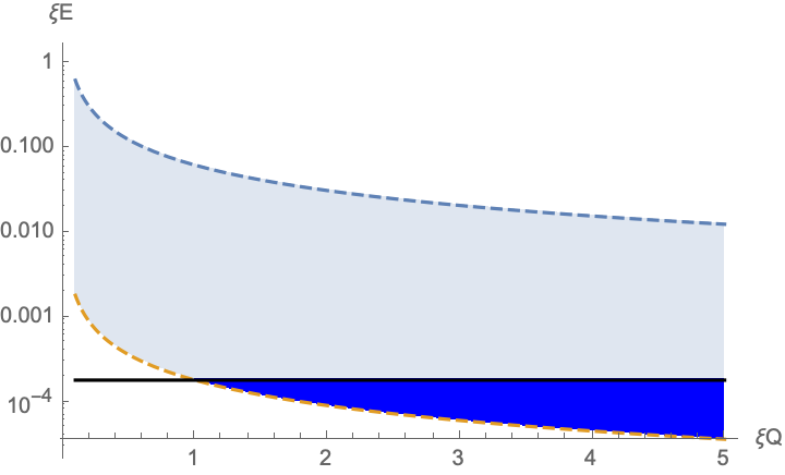
Figure 4: Sketch of the parameter space $\xi_{Q}$ and $\xi_{E}$. The bright blue region satisfies the two conditions (53 and 54), which are represented by the dashed lines (blue for 53 and orange for 54). The condition (55) is saturated at the black line, such that the dark blue region satisfies all three conditions ((53, 54, and 55). Here, $\Delta E_{m}=20\,\mathrm{keV}$. The gray dotted line is for $t_{bottle}=15\,\mathrm{s}$, which corresponds to the limiting case, when the intersection of (55) and condition (54) becomes to large to be realized by simple dipoles within a neutron radius.

One realizes from this figure that the parameter space is quite constrained, giving minimal and maximal values for both $\xi_{E}$ and $\xi_{Q}$. This also figure illustrates two more interesting aspects: First, the minimal value of $\xi_{Q}$ of the deep blue region is of the order of one, which is surprisingly close to a naive estimate of the quadrupole moment. Second, for reasonable values of $\xi_{Q}<4$, the gray dotted curve suggests that the electromagnetic transition time is more on the bottle end of the window between the beam time and the bottle time

$$15\,\mathrm{s}<\tau_{\gamma}<300\,\mathrm{s}.$$ (56)

Keeping in mind that we were working with a very bold model, the obtained regions for $\xi_{E}$ and $f_{r}$ are quite reasonable.

IV.3 Analogies

The characteristics of an excited state that has a longer lifetime than the ground state, as proposed here for the free neutron, is quite unusual. Nevertheless there are some cases with this characteristics known in nuclear physics. Interestingly, nuclear isomers become metastable, if the spin structure between excited and ground state is largely different. For example, certain nuclear isomers, such as ^180mTa are stable in contrast to their ground state Lehnert:2016iku . Also only recently, other isomers with only tiny excitation energy have been discovered Sikorsky:2020peq .

Another analogy in nuclear physics can be found in the magnetic dipole interactions of currents within atomic nuclei. In these nuclei it is also magnetic dipoles and exchange currents that are responsible for the existence of excited states of otherwise degenerate states with the same nuclear mass Heyde:2010ng . In this context we also want to mention the resonance that was found in polarized neutron - proton scattering WASA-at-COSY:2014dmv .

IV.4 How to test the hypothesis?

The hypothesis of an excited state in the context of the N$\lambda$P can be tested directly. Such tests would involve designing experiments or observations aimed at detecting the predicted characteristics of this state. Here are several potential approaches to test the hypothesis directly:

• Perform a beam experiment at later time, which means constructing longer beam pipes with length $L$. Check whether the deduced decay time depends on $L$. This narrows the window between $t_{\mathrm{beam}}=L/v_{n}$ and $t_{\mathrm{bottle}}$ from below.

• Repeat a bottle experiment at earlier times $t_{\mathrm{bottle}}$. Check whether the deduced decay time depends on $t_{\mathrm{bottle}}$. This narrows the window from above. For our toy model we expect relatively large values for $\tau_{\gamma}$ (56), which speaks for this method.

• Search for electromagnetic signatures of the transition between $\Psi_{e}$ and $\Psi_{g}$ along beam pipes, UCN cooling facilities, or before filling UCN bottle containers RDKII:2016lpd ; Cooper:2010zza ; Tang:2018eln . For example, correlations between $\gamma$ backgrounds from neutron beams have been measured and compared to simulations to a few percent level CSNS:2020 . Such backgrounds will be of crucial importance. If for instance $\tau_{\gamma}\approx t_{\mathrm{beam}}$ then the signature will have to compete with the background of reactor photons. Instead, if $\tau_{\gamma}\approx t_{\mathrm{bottle}}$ like in (56), the signal will have to compete with the background generated by secondary reactions of the actual weak decays.

• Try to re-populate the excited state with fine-tuned external radiation.

• Recalculate the angular distributions of the neutron decay products in analogy to (33 and 38) and compare to the nucleon decay parameters measured e.g. in Reich:2000au ; Klopf:2019afh .

Apart from these tests, one can also look for indirect signatures in all sorts of precision experiments with free neutrons, as long as these experiments are performed at $t<t_{\mathrm{bottle}}$. Other neutron rich environments such as the early universe during Big Bang Nucleosynthesis, or neutron stars, are probably insensitive to the seeing the excited state due to the immense red-shift of the former and the huge gravitational binding energy of the latter.

One interesting test opportunity we want to mention also is the systematic $3.9\sigma$ energy shift observed in the qBounce experiment Micko:2023oar . Since the energies in qBounce depend on the neutron mass, this relative shift of $\approx 10^{-3}$ could be associated to a mass shift due to an excited state.

V Conclusion

In this paper we revisited the neutron lifetime puzzle, assuming that both mutual contradicting experimental results are correct. Our exploration has led us to propose a novel perspective on the N$\lambda$P. The discrepancy could be explained if: The conditions (a–f) from section II are fulfilled. We then presented a three-quark toy model utilizing the spin configurations (15) and (16). Through this model, we demonstrated that the conditions a)-d) can be satisfied quite naturally, while e) and f) are posed as additional assumption.

It is crucial to note that our presented toy model is intended to serve as a starting point for further exploration rather than a definitive explanation. Our primary goal is to emphasize the possibility that the N$\lambda$P may suggest the presence of an excited state with the outlined characteristics. While a substantial portion of our effort went into constructing and discussing a specific model, we encourage further investigations and alternative approaches to validate and refine our proposed hypothesis of an excited state.

In essence, this study opens a pathway for future research to delve deeper into the nature of neutron decay and the potential existence of an excited states, providing valuable insights that could contribute to resolving the Neutron Lifetime Puzzle.

References

- (1) R. L. Workman et al. [Particle Data Group], PTEP 2022 (2022), 083C01 doi:10.1093/ptep/ptac097
- (2) W. Heisenberg, Z. Phys. 77 (1932), 1-11 doi:10.1007/BF01342433
- (3) E. Wigner, Phys. Rev. 51 (1937), 106-119 doi:10.1103/PhysRev.51.106
- (4) W. Greiner, B. Mueller, Springer, doi:10.1007/978-3-540-87843-8.
- (5) M. Lavelle and D. McMullan, Phys. Rept. 279 (1997), 1-65 doi:10.1016/S0370-1573(96)00019-1 [arXiv:hep-ph/9509344 [hep-ph]].
- (6) G. Eichmann, H. Sanchis-Alepuz, R. Williams, R. Alkofer and C. S. Fischer, Prog. Part. Nucl. Phys. 91 (2016), 1-100 doi:10.1016/j.ppnp.2016.07.001 [arXiv:1606.09602 [hep-ph]].
- (7) A. Deur, S. J. Brodsky and G. F. De Téramond, doi:10.1088/1361-6633/ab0b8f [arXiv:1807.05250 [hep-ph]].
- (8) G. Veneziano, Mod. Phys. Lett. A 4 (1989), 1605 doi:10.1142/S0217732389001830
- (9) M. Anselmino, B. L. Ioffe and E. Leader, Sov. J. Nucl. Phys. 49 (1989), 136 NSF-ITP-88-94.
- (10) G. C. Nayak, JHEP 03 (2018), 101 doi:10.1007/JHEP03(2018)101 [arXiv:1802.02864 [hep-ph]].
- (11) C. E. Carlson, Prog. Part. Nucl. Phys. 82 (2015), 59-77 doi:10.1016/j.ppnp.2015.01.002 [arXiv:1502.05314 [hep-ph]].
- (12) D. F. Geesaman, K. Saito and A. W. Thomas, Ann. Rev. Nucl. Part. Sci. 45 (1995), 337-390 doi:10.1146/annurev.ns.45.120195.002005
- (13) S. Paul, Nucl. Instrum. Meth. A 611, 157 (2009) doi:10.1016/j.nima.2009.07.095 [arXiv:0902.0169 [hep-ex]].
- (14) A. P. Serebrov and A. K. Fomin, Phys. Procedia 17 (2011), 199-205 doi:10.1016/j.phpro.2011.06.037 [arXiv:1104.4238 [nucl-ex]].
- (15) F. E. Wietfeldt and G. L. Greene, Rev. Mod. Phys. 83, no. 4, 1173 (2011). doi:10.1103/RevModPhys.83.1173
- (16) A. P. Serebrov et al., KnE Energ. Phys. 3, 121 (2018). doi:10.18502/ken.v3i1.1733
- (17) F. M. Gonzalez et al. [UCN], Phys. Rev. Lett. 127 (2021) no.16, 162501 doi:10.1103/PhysRevLett.127.162501 [arXiv:2106.10375 [nucl-ex]].
- (18) R. W. Pattie, Jr. et al., Science 360, no. 6389, 627 (2018) doi:10.1126/science.aan8895 [arXiv:1707.01817 [nucl-ex]].
- (19) V. F. Ezhov et al., JETP Lett. 107, no. 11, 671 (2018) [Pisma Zh. Eksp. Teor. Fiz. 107, no. 11, 707 (2018)] doi:10.1134/S0021364018110024, 10.7868/S0370274X18110036 [arXiv:1412.7434 [nucl-ex]].
- (20) I. Altarev, C. A. Baker, G. Ban, K. Bodek, M. Daum, P. Fierlinger, P. Geltenbort, K. Green, M. G. D. van der Grinten and E. Gutsmiedl, et al. Phys. Rev. D 80 (2009), 032003 doi:10.1103/PhysRevD.80.032003 [arXiv:0905.4208 [nucl-ex]].
- (21) Z. Berezhiani, Eur. Phys. J. C 79, no. 6, 484 (2019) doi:10.1140/epjc/s10052-019-6995-x [arXiv:1807.07906 [hep-ph]].
- (22) Z. Berezhiani and A. Vainshtein, Phys. Lett. B 788, 58 (2019) doi:10.1016/j.physletb.2018.11.014 [arXiv:1809.00997 [hep-ph]].
- (23) W. Tan, Universe 9 (2023) no.4, 180 doi:10.3390/universe9040180 [arXiv:2302.07805 [nucl-ex]].
- (24) L. J. Broussard, J. L. Barrow, L. DeBeer-Schmitt, T. Dennis, M. R. Fitzsimmons, M. J. Frost, C. E. Gilbert, F. M. Gonzalez, L. Heilbronn and E. B. Iverson, et al. Phys. Rev. Lett. 128 (2022) no.21, 212503 doi:10.1103/PhysRevLett.128.212503 [arXiv:2111.05543 [nucl-ex]].
- (25) G. Dvali, M. Ettengruber and A. Stuhlfauth, [arXiv:2312.13278 [hep-ph]].
- (26) B. Belfatto, R. Beradze and Z. Berezhiani, Eur. Phys. J. C 80 (2020) no.2, 149 doi:10.1140/epjc/s10052-020-7691-6 [arXiv:1906.02714 [hep-ph]].
- (27) D. Barducci, M. Fabbrichesi and E. Gabrielli, Phys. Rev. D 98 (2018) no.3, 035049 doi:10.1103/PhysRevD.98.035049 [arXiv:1806.05678 [hep-ph]].
- (28) A. P. Serebrov, M. E. Chaikovskii, G. N. Klyushnikov, O. M. Zherebtsov and A. V. Chechkin, Phys. Rev. D 103 (2021) no.7, 074010 doi:10.1103/PhysRevD.103.074010 [arXiv:2011.13272 [nucl-ex]].
- (29) F. E. Wietfeldt, R. Biswas, J. Caylor, B. Crawford, M. S. Dewey, N. Fomin, G. L. Greene, C. C. Haddock, S. F. Hoogerheide and H. P. Mumm, et al. Phys. Rev. D 107 (2023) no.11, 118501 doi:10.1103/PhysRevD.107.118501
- (30) M. Klopf, E. Jericha, B. Märkisch, H. Saul, T. Soldner and H. Abele, Phys. Rev. Lett. 122, no. 22, 222503 (2019) doi:10.1103/PhysRevLett.122.222503 [arXiv:1905.01912 [hep-ex]].
- (31) D. Dubbers, H. Saul, B. Märkisch, T. Soldner and H. Abele, Phys. Lett. B 791, 6 (2019) doi:10.1016/j.physletb.2019.02.013 [arXiv:1812.00626 [nucl-ex]].
- (32) J. I. Collar and C. M. Lewis, [arXiv:2203.00750 [physics.ins-det]].
- (33) A. N. Khan, Nucl. Phys. B 986 (2023), 116064 doi:10.1016/j.nuclphysb.2022.116064 [arXiv:2201.10578 [hep-ph]].
- (34) S. Weinberg, Phys. Rev. 112 (1958), 1375-1379 doi:10.1103/PhysRev.112.1375
- (35) B. Fornal, Universe 9 (2023) no.10, 449 doi:10.3390/universe9100449 [arXiv:2306.11349 [hep-ph]].
- (36) J. Byrne, “An overview of neutron decay,” International Workshop on Quark Mixing, CKM Unitarity, 15-25, www.physi.uni-heidelberg.de/Publications/ckmbyrne.pdf
- (37) T. Tatsumi, Phys. Lett. B 489 (2000), 280-286 doi:10.1016/S0370-2693(00)00927-8 [arXiv:hep-ph/9910470 [hep-ph]].
- (38) T. Maruyama and T. Tatsumi, Nucl. Phys. A 693 (2001), 710-730 doi:10.1016/S0375-9474(01)00811-9 [arXiv:nucl-th/0010018 [nucl-th]].
- (39) T. Tatsumi, T. Maruyama and E. Nakano, Prog. Theor. Phys. Suppl. 153 (2004), 190-197 doi:10.1143/PTPS.153.190 [arXiv:hep-ph/0312347 [hep-ph]].
- (40) A. Niegawa, Prog. Theor. Phys. 113 (2005), 581-601 doi:10.1143/PTP.113.581 [arXiv:hep-ph/0404252 [hep-ph]].
- (41) V. V. Nesvizhevsky, H. G. Borner, A. M. Gagarski, A. K. Petoukhov, G. A. Petrov, H. Abele, S. Baessler, G. Divkovic, F. J. Ruess and T. Stoferle, et al. Phys. Rev. D 67 (2003), 102002 doi:10.1103/PhysRevD.67.102002 [arXiv:hep-ph/0306198 [hep-ph]].
- (42) T. Jenke, P. Geltenbort, H. Lemmel and H. Abele, Nature Phys. 7 (2011), 468-472 doi:10.1038/nphys1970
- (43) B. Lehnert, M. Hult, G. Lutter and K. Zuber, Phys. Rev. C 95 (2017) no.4, 044306 doi:10.1103/PhysRevC.95.044306 [arXiv:1609.03725 [nucl-ex]].
- (44) T. Sikorsky, J. Geist, D. Hengstler, S. Kempf, L. Gastaldo, C. Enss, C. Mokry, J. Runke, C. E. Düllmann and P. Wobrauschek, et al. Phys. Rev. Lett. 125 (2020) no.14, 142503 doi:10.1103/PhysRevLett.125.142503 [arXiv:2005.13340 [nucl-ex]].
- (45) K. Heyde, P. von Neumann-Cosel and A. Richter, Rev. Mod. Phys. 82 (2010), 2365-2419 doi:10.1103/RevModPhys.82.2365 [arXiv:1004.3429 [nucl-ex]].
- (46) P. Adlarson et al. [WASA-at-COSY], Phys. Rev. Lett. 112 (2014) no.20, 202301 doi:10.1103/PhysRevLett.112.202301 [arXiv:1402.6844 [nucl-ex]].
- (47) M. J. Bales et al. [RDK II], Phys. Rev. Lett. 116 (2016) no.24, 242501 doi:10.1103/PhysRevLett.116.242501 [arXiv:1603.00243 [nucl-ex]].
- (48) R. L. Cooper, T. E. Chupp, M. S. Dewey, T. R. Gentile, H. P. Mumm, J. S. Nico, A. K. Thompson, B. M. Fisher, I. Kremsky and F. E. Wietfeldt, et al. Phys. Rev. C 81 (2010), 035503 doi:10.1103/PhysRevC.81.035503
- (49) Z. Tang, M. Blatnik, L. J. Broussard, J. H. Choi, S. M. Clayton, C. Cude-Woods, S. Currie, D. E. Fellers, E. M. Fries and P. Geltenbort, et al. Phys. Rev. Lett. 121 (2018) no.2, 022505 doi:10.1103/PhysRevLett.121.022505 [arXiv:1802.01595 [nucl-ex]].
- (50) Qiang Li et. al Nuclear Instruments and Methods in Physics Research Section A: 980 (2020) 164506 doi:10.1016/j.nima.2020.164506 .
- (51) J. Reich, H. Abele, M. A. Hoffmann, S. Baessler, P. von Bulow, D. Dubbers, U. Peschke, V. Nesvizhevsky and O. Zimmer, Nucl. Instrum. Meth. A 440 (2000), 535-538 doi:10.1016/S0168-9002(99)01032-3
- (52) M. Klopf, E. Jericha, B. Märkisch, H. Saul, T. Soldner and H. Abele, Phys. Rev. Lett. 122 (2019) no.22, 222503 doi:10.1103/PhysRevLett.122.222503 [arXiv:1905.01912 [hep-ex]].
- (53) J. Micko, F. Di Pumpo, J. Bosina, S. S. Cranganore, T. Jenke, M. Pitschmann, S. Roccia, R. I. P. Sedmik and H. Abele, [arXiv:2203.16375 [gr-qc]].