VisRec: A Semi-Supervised Approach to Radio Interferometric Data Reconstruction

Abstract

Radio telescopes produce visibility data about celestial objects, but these data are sparse and noisy. As a result, images created on raw visibility data are of low quality. Recent studies have used deep learning models to reconstruct visibility data to get cleaner images. However, these methods rely on a substantial amount of labeled training data, which requires significant labeling effort from radio astronomers. Addressing this challenge, we propose VisRec, a model-agnostic semi-supervised learning approach to the reconstruction of visibility data. Specifically, VisRec consists of both a supervised learning module and an unsupervised learning module. In the supervised learning module, we introduce a set of data augmentation functions to produce diverse training examples. In comparison, the unsupervised learning module in VisRec augments unlabeled data and uses reconstructions from non-augmented visibility data as pseudo-labels for training. This hybrid approach allows VisRec to effectively leverage both labeled and unlabeled data. This way, VisRec performs well even when labeled data is scarce. Our evaluation results show that VisRec outperforms all baseline methods in reconstruction quality, robustness against common observation perturbation, and generalizability to different telescope configurations.

1 Introduction

In radio astronomy, a radio interferometer consists of an array of antennas, all observing the same area of sky, forming a single, unified telescope. The visibility refers to the signal obtained by cross-correlating pairs of antennas, which is in the frequency domain. Visibility data are then used to construct images of the celestial objects being observed Dagli (2023). Due to the incompleteness and noise in the visibility data, the resultant images, known as dirty images, are often dominated by artifacts Schmidt et al. (2022). As a result, radio interferometric data must be reconstructed before being used in scientific analysis. In this paper, we introduce a semi-supervised method to reconstruct the visibility.

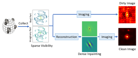
Figure 1: Illustration of radio interferometric data processing. The telescopes collect visibility data. The imaging results of the raw data is dominated by artifacts, called dirty images. In contrast, the imaging results of sparse-to-dense reconstructed visibility data are cleaner.

Recently, many deep-learning methods have shown promising reconstruction results on synthetic datasets Sun and Bouman (2021); Connor et al. (2022); Wu et al. (2022); Schmidt et al. (2022); Wang et al. (2023); Geyer et al. (2023). These methods address radio interferometric data reconstruction as a supervised learning problem in which the reconstruction error between the predicted results and the reference labels is minimized Jia et al. (2022). However, these deep-learning-based methods are highly dependent on a great amount of ground truth (labels) for model training, and obtaining ground truth data is difficult. In contrast to natural or medical image reconstruction, where long-time scanning can produce fully-sampled (labeled) training data, obtaining a fully-sampled sky measurement dataset via radio telescopes is impractical due to observational constraints. Furthermore, it takes expertise and human labor to get a ground truth clean image. As such, techniques that can leverage information from unlabeled datasets are indispensable where ground-truth images are scarce.

Another problem that often comes with the scarcity of labeled data is limited robustness and generalizability in supervised-learning-based reconstruction methods, due to the lack of diversity in training data Darestani et al. (2021); Desai et al. (2023). In particular, existing radio interferometry data reconstructing methods focus on enhancing reconstruction accuracy, and are sensitive to data distribution shift. We followed previous studies Schmidt et al. (2022); Darestani et al. (2021) to generate test data with errors caused by noise perturbations during observation or offline antennas as well as data collected from different telescope configurations. Our results confirm the low robustness and generalizability of existing methods.

To address these problems, we propose a model-agnostic semi-supervised learning approach to radio interferometry data reconstruction, called VisRec. Specifically, VisRec consists of two modules: a supervised learning module and an unsupervised learning module. The supervised module integrates a variety of data augmentation functions, exposing the model to diverse training examples. The unsupervised module applies augmentations to unlabeled visibility data and employs reconstructions from non-augmented data as pseudo-labels. VisRec computes the consistency loss between the reconstruction of augmented visibilities and the pseudo-labels to lead the model to be more robust against perturbations. Our method effectively leverages both labeled and unlabeled data to improve model performance.

The main contributions of our work are:

• We propose VisRec, which is the first model-agnostic semi-supervised framework for radio interferometric data reconstruction. By combining supervised and unsupervised learning modules, VisRec successfully leverages both labeled and unlabeled data, reducing the dependency on ground truth labels.

• We empirically show that our method is robust to common observation perturbation, and has good generalizability when applied to data from different telescope configurations.

• We introduce a variety of data augmentation methods for visibility data, including both label-invariant and label-variant augmentations. These augmentations improve the model performance when applied to VisRec as well as supervised learning methods.

2 Background and Related Work

2.1 Radio Interferometric Imaging

In radio astronomy, observing distant astronomical objects via radio interferometry demands large-aperture telescopes, as the angular resolution is inversely related to aperture size Bouman et al. (2018). High angular resolution can be obtained using the technique of Very Long Baseline Interferometry (VLBI). VLBI uses a network of globally distributed radio telescopes to create a unified Earth-size telescope. Individual telescopes record radio waves from space, and these signals are then cross-correlated between antenna pairs to produce visibility data. The resulting visibility data is inherently sparse due to the limited number of antennas in VLBI Thompson et al. (2017); Bouman et al. (2018).

Visibility data is in the form of complex values in the uv-plane, a geometric plane defined for interferometric observations. The imaging process is an inverse Fourier transformation, translating $(u,v)$ coordinates in the frequency domain into $(l,m)$ coordinates in the image domain Wu et al. (2022), represented by the equation:

$$I(l,m) = \int_{u}\int_{v}e^{2\pi i(ul+vm)}V(u,v)dudv.$$ (1)

Here, $V(u,v)$ denotes visibility data in the frequency domain, and $I(l,m)$ is the intensity distribution of the sky in the image domain.

2.2 Interferometric Data Reconstruction

The imaging results of the under-sampled sparse visibility data are dominated by artifacts so the data must be reconstructed before being used in scientific research Schmidt et al. (2022). Interferometric image reconstruction is an ill-posed problem because there are infinite solution images that fit the observed visibility Sun and Bouman (2021). Traditional methods, particularly the CLEAN method Högbom (1974), have been widely used for this task. CLEAN iteratively refines dirty images to differentiate actual celestial structures from artifacts. However, the performance of CLEAN is limited due to its assumption of point-like sources and long inference time Connor et al. (2022). Recently, some deep-learning-based data processing methods have been proposed for radio interferometric data reconstruction. Some of them first transfer the sparse visibility data into dirty images through the imaging process and then reconstruct the dirty images into clean images Bouman et al. (2016); Sun and Bouman (2021); Connor et al. (2022). In contrast, some recent deep learning-based studies Schmidt et al. (2022); Wu et al. (2022); Geyer et al. (2023) have proposed to first do inpainting on the visibility data to reconstruct the sparse samples into dense coverage, and then perform imaging to obtain the clean image, showing better performance. However, existing deep-learning methods for interferometric data reconstruction are based on supervised learning, which requires a great amount of training data and does not leverage unlabeled measurements. In this paper, we adopt the reconstruction-and-imaging processing flow and propose a semi-supervised method to leverage both labeled and unlabeled data.

3 Our Method

3.1 Problem Formulation

In radio astronomy, the task of recovering the brightness distribution of the real sky from the observed visibility data is an inverse problem Sun and Bouman (2021). Consider an image $x\in\mathbb{R}^{n}$ representing the brightness distribution of the sky, and its corresponding sampled visibility $v\in\mathbb{R}^{m}$. They follow the forward model:

$$v=\mathbf{P}_{\Omega}F(x)+\widetilde{\epsilon}.$$ (2)

In this model, $F$ denotes the Fourier transformation, $\mathbf{P}_{\Omega}\in\mathbb{R}^{m\times n}$ is an under-sampling matrix where $\Omega$ is the telescope’s sampling pattern, and $\widetilde{\epsilon}$ denotes noise with the same dimension as $v$. In this paper, our goal is to first estimate the full visibility data $F(x)$ from the observed sparse visibility data, and then apply inverse Fourier transform $F^{-1}$ to estimate the final clean image $x$ of the brightness distribution of real sky.

Consider a dataset $\mathcal{D}=\mathcal{D}^{(s)}\cup\mathcal{D}^{(u)}$. $\mathcal{D}^{(s)}$ denotes the subset consisting of sparse visibility samples as well as corresponding ground truth images for supervised learning. $v^{(s)}_{i}\in\mathcal{D}^{(s)}$ is the sparse visibility measurement of the $i^{th}$ example in $\mathcal{D}^{(s)}$. $x^{(s)}_{i}\in\mathcal{D}^{(s)}$ is the image ground truth corresponding to $v^{(s)}_{i}$. $\mathcal{D}^{(u)}$ is the subset including sparse visibility data lacking ground truth labels for unsupervised learning. $v^{(u)}_{j}\in\mathcal{D}^{(u)}$ is the $j^{th}$ example of sparse visibility measurement in $\mathcal{D}^{(u)}$. The reconstruction model, denoted by $f_{\theta}$, is parameterized by $\theta$. $|\cdot|$ denotes the dataset size. In radio astronomical observation, the size of the supervised dataset $|\mathcal{D}^{(s)}|$ is smaller than the unsupervised dataset $|\mathcal{D}^{(u)}|$.

Figure 2: Overview of our method. In our semi-supervised framework, labeled data undergo supervised training, as depicted by the blue arrows. The labeled data are augmented with label-variant and label-invariant augmentations $T_{var}$ and $T_{inv}$. Then the neural network, denoted by $f_{\theta}$, processes augmented visibility data to produce reconstructions. These reconstructions are then compared against ground-truth references to compute supervised loss $\mathcal{L}_{sup}$. Unlabeled sparse visibility data are augmented by $T_{corr}$, and the same $f_{\theta}$ reconstructs both the non-augmented and augmented visibility data. The reconstruction from the non-augmented unlabeled data serves as a pseudo-label for that with augmentations to compute the consistency loss $\mathcal{L}_{cons}$. The overall loss combines supervised and consistency losses in a weighted sum: $\mathcal{L}_{total}\leftarrow\mathcal{L}_{sup}+\lambda\mathcal{L}_{cons}$.

3.2 Label-Efficient Reconstruction of Visibility

We introduce VisRec, a semi-supervised learning framework that employs an arbitrary learnable reconstruction model $f_{\theta}$, parameterized by weights $\theta$, to reconstruct the visibility data into dense inpaintings. Then the dense inpaintings are used to produce high-fidelity clean images. VisRec consists of two modules, a supervised module and an unsupervised module.

3.2.1 Supervised Module

In supervised radio interferometry data reconstruction, learning-based models are trained with datasets where reference clean images are available, denoted as $\mathcal{D}^{(s)}$. For each instance, the ground-truth clean image $x$ is transformed into the reference visibility data $F(x)$ to be compared with sparse visibility $v_{i}^{(s)}$. Here, $F$ is the transformation from the image domain to the visibility domain. The training objective of the model $f_{\theta}$ is to minimize the supervised loss function:

$$\min_{\theta}\frac{1}{|\mathcal{D}^{(s)}|}\sum_{i=0}^{|\mathcal{D}^{(s)}|}\mathcal{L}_{sup}\left(f_{\theta}\left(v_{i}^{(s)}\right),F\left(x_{i}^{(s)}\right)\right)$$ (3)

where $\mathcal{L}_{sup}$ represents the supervised loss function. The model $f_{\theta}$ refers to any parameterized learnable model.

To improve data diversity in label-scarce scenarios, supervised reconstruction techniques can employ data augmentation strategies. We define a series of label-invariant augmentation functions ${T_{inv,l}},{l=1}...{m}$ and label-variant augmentation functions ${T_{var,k}},{k=1}...{n}$, each applied to the visibility data with a certain probability:

$$T_{inv}(v_{i}^{(s)})=T_{inv,1}^{(p_{1})}\circ\ldots\circ T_{inv,m}^{(p_{m})}(v_{i}^{(s)})$$ (4)

$$T_{var}(v_{i}^{(s)},x_{i}^{(s)})=T_{var,1}^{(q_{1})}\circ\ldots\circ T_{var,n}^{(q_{n})}(v_{i}^{(s)},x_{i}^{(s)})$$ (5)

where $p_{j},q_{k}$ are the probabilities of applying each augmentation function.

The augmented loss for an instance with label-invariant visibility augmentation is:

$$\mathcal{L}_{sup}\left(f_{\theta}\left(T_{inv}\left(v_{i}^{(s)}\right)\right),F\left(x_{i}^{(s)}\right)\right).$$ (6)

The augmented loss for an instance with label-variant visibility augmentation is:

$$\mathcal{L}_{sup}\left(f_{\theta}\left(v_{i}^{\prime{(s)}}\right),F\left(x_{i}^{\prime{(s)}}\right)\right)$$ (7)

where

$${v}^{\prime(s)}_{i},{x}^{\prime(s)}_{i}=T_{var}(v^{(s)}_{i},x^{(s)}_{i}).$$ (8)

This dual augmentation approach ensures that the learnable models are trained with a comprehensive range of variations. Suppose an instance of sparse visibility observation is in the form of $\{u_{s},v_{s},{V}\left(u_{s},v_{s}\right)\}$, where $u_{s}$ and $v_{s}$ are coordinates at which a measurement is sampled, and ${V}\left(u_{s},v_{s}\right)$ is the complex value of the sample. For label-invariant visibility augmentation, we introduce the following methods:

• Position Offset:

  $$(u_{s}^{\prime},v_{s}^{\prime})=(u_{s},v_{s})+\epsilon_{pos}$$ (9)

  where $\epsilon_{pos}\in\mathbb{R}^{\text{shape}((u_{s},v_{s}))}\sim\mathcal{N}(0,\sigma_{\text{pos}})$ is Gaussian noise added to the position coordinates.

• Visibility Noise:

  $$V^{\prime}(u_{s},v_{s})=V(u_{s},v_{s})+\epsilon_{vis}$$ (10)

  where $\epsilon_{vis}\in\mathbb{C}^{\text{shape}(V(u_{s},v_{s}))}\sim\mathcal{N}(0,\sigma_{vis})$ is complex Gaussian noise added to the visibility values.

• Global Position Offset:

  $$(u_{s}^{\prime},v_{s}^{\prime})=(u_{s},v_{s})+(\Delta u,\Delta v)$$ (11)

  where $(\Delta u,\Delta v)$ is a uniform random offset applied to all position coordinates.

• Random Cropping: A random subset of visibility data is dropped out.

• Subset of Selective Frequency: The selected sampling subset is represented as:

  $$\left\{(u_{s},v_{s},V(u_{s},v_{s}))\,\bigg{|}\,d_{\text{min}}\leq\sqrt{u_{s}^{2}+v_{s}^{2}}\leq d_{\text{max}}\right\}$$

  where $d_{\text{min}}$ and $d_{\text{max}}$ are the minimum and maximum frequencies of the selected range.

For label-variant visibility augmentation, we introduce some geometric transformations in the uv-plane. To augment sparsely sampled visibility data $\{u_{s},v_{s},{V}\left(u_{s},v_{s}\right)\}$ while maintaining correspondence with the image ground-truth $x$, the augmentations must be consistent across both the visibility data and the image domain:

• Transpose Transformation: Swap $u_{s}$ and $v_{s}$ coordinates for the visibility data while apply a 90-degree rotation to the clean image $x$.

• Reflection: Negate the $u_{s}$ or $v_{s}$ coordinates in the visibility data. For the clean image $x$, apply a horizontal or vertical flip.

• Central Symmetry Transformation: Negate both $u_{s}$ and $v_{s}$ in the visibility data and apply a central inversion to the clean image $x$.

We design these augmentations following traditional image augmentation techniques Xu et al. (2023) and adapt them to the properties of visibility data.

3.2.2 Unsupervised Module

The unsupervised module of VisRec uses unlabeled visibility data $\mathcal{D}^{(u)}$ that miss ground-truth images. Our aim is to leverage these data to train the model $f_{\theta}$ to recover the original signal from a corruption-augmented measurement Desai et al. (2023). Each unsupervised example $v^{(u)}_{i}$ is augmented by a predefined signal corruption model $T_{corr}$, which simulates expected corrupted patterns that occur in radio interferometry observations. The corruption model $T_{corr}$ applied to each unsupervised instance simulates a variety of realistic observational impairments:

• Observation Noise Schmidt et al. (2022): Introducing zero-mean Gaussian noise to simulate electronic and atmospheric noise.

• Missing Data Nasirudin et al. (2022): Simulating the effect of offline antennas by masking out some visibility points.

• Antenna Offset Nasirudin et al. (2022): Introducing perturbations that represent errors in antenna positioning or alignment by adding noise to the positional coordinates.

Similar to label-invariant visibility augmentation in the supervised learning module, $T_{corr}$ is also applied to the visibility data with a predefined probability.

The unsupervised training objective is to minimize the following loss function:

$$\min_{\theta}\frac{1}{|\mathcal{D}^{(u)}|}\sum_{j=0}^{|\mathcal{D}^{(u)}|}\mathcal{L}_{cons}\left(f_{\theta}\left(T_{corr}(v^{(u)}_{j})\right),f_{\theta}\left(v^{(u)}_{j}\right)\right)$$ (12)

This approach trains the model to reconstruct the corrupted visibility by learning to reverse the effects of the corruption-augmentation, which we refer to as consistency training.

3.2.3 Semi-Supervised Training

VisRec consists of both supervised learning and unsupervised learning processes. The main framework of our method is described in Algorithm 1. In the supervised process, we sample a batch of $\{(v^{(s)}_{i},x^{(s)}_{i})\}_{i=1}^{N_{s}}$ from $\mathcal{D}^{(s)}$. The visibility data $v^{(s)}_{i}$ and ground-truth image labels $x^{(s)}_{i}$ are augmented by label-variant augmentation function $T_{var}$. Then the visibility data is augmented by label-invariant augmentation function $T_{inv}$. Then the model $f_{\theta}$ generates the reconstruction of input visibility data.

In the unsupervised process, we sample the batch $\{v^{(u)}_{j}\}_{j=1}^{N_{u}}$ from $\mathcal{D}^{(u)}$. Then each $v^{(u)}_{j}$ is augmented by corruption model $T_{corr}$. Finally, the same model $f_{\theta}$ reconstructs both augmented and original visibility.

Finally, a supervised loss $\mathcal{L}_{sup}$ is computed using the mean squared error between the Fourier-transformed ground truth images and the reconstructed visibility data for the supervised subset. Meanwhile, a consistency loss $\mathcal{L}_{cons}$ is calculated for the unsupervised data by comparing the model’s output on the original and augmented visibility samples. The total loss $\mathcal{L}_{total}$ is a weighted sum of these two losses, where $\lambda$ is a hyperparameter that balances the two components. The model parameters $\theta$ are updated by backpropagation to minimize $\mathcal{L}_{total}$.

Algorithm 1 Main process of VisRec.

Input: Dataset $\mathcal{D}=\mathcal{D}^{(s)}\cup\mathcal{D}^{(u)}$
Output: Trained model $f_{\theta}$

1:  for each sampled batch $\{(v^{(s)}_{i},x^{(s)}_{i})\}_{i=1}^{N_{s}}$ and $\{v^{(u)}_{j}\}_{j=1}^{N_{u}}$ do

2:     for all $i\in\{1,\ldots,N_{s}\}$ do

3:        ${v}^{\prime(s)}_{i},{x}^{\prime(s)}_{i}\leftarrow T_{var}(v^{(s)}_{i},x^{(s)}_{i})$

4:        $\tilde{v}^{(s)}_{i}\leftarrow f_{\theta}(T_{inv}(v^{\prime(s)}_{i}))$

5:     end for

6:     for all $j\in\{1,\ldots,N_{u}\}$ do

7:        $\tilde{v}^{(u)}_{j}\leftarrow f_{\theta}(v^{(u)}_{j})$

8:        $\hat{v}^{(u)}_{j}\leftarrow f_{\theta}(T_{corr}({v}^{(u)}_{j}))$

9:     end for

10:     $\mathcal{L}_{sup}\leftarrow\frac{1}{N_{s}}\sum_{i=1}^{N_{s}}\mathcal{L}_{sup}(F(x^{\prime(s)}_{i}),\tilde{v}^{(s)}_{i})$

11:     $\mathcal{L}_{cons}\leftarrow\frac{\lambda}{N_{u}}\sum_{j=1}^{N_{u}}\mathcal{L}_{cons}(\hat{v}^{(u)}_{j},\tilde{v}^{(u)}_{j})$

12:     $\mathcal{L}_{total}\leftarrow\mathcal{L}_{sup}+\lambda\mathcal{L}_{cons}$

13:     Update network $f_{\theta}$ to minimize $\mathcal{L}_{total}$

14:  end for

15:  return $f_{\theta}$

Table 1: Comparison of image reconstruction quality on EHT and VLBA datasets (mean and standard deviation). Rows with gray background denote our method and its variants, and the rows with white background represent methods from prior studies.

	EHT Dataset			VLBA Dataset
Method	LFD ($\downarrow$)	SSIM ($\uparrow$)	PSNR (dB) ($\uparrow$)	LFD ($\downarrow$)	SSIM ($\uparrow$)	PSNR (dB) ($\uparrow$)
Dirty Image	N/A	0.685 (0.059)	10.58 (1.28)	N/A	0.745 (0.041)	12.24 (1.34)
CLEAN Högbom (1974)	N/A	0.830 (0.032)	19.17 (2.61)	N/A	0.823 (0.031)	18.48 (2.52)
Noise2Astro Zhang et al. (2022)	N/A	0.704 (0.055)	11.09 (1.36)	N/A	0.761 (0.034)	13.08 (1.37)
Neural Field Wu et al. (2022)	1.083 (0.328)	0.875 (0.030)	21.36 (2.51)	1.152 (0.312)	0.874 (0.032)	20.26 (2.60)
NF Supervised + Aug	1.043 (0.343)	0.883 (0.028)	21.89 (2.47)	1.083 (0.334)	0.888 (0.030)	21.24 (2.75)
NF Self-Supervised	1.465 (0.234)	0.703 (0.056)	11.45 (1.45)	1.433 (0.239)	0.766 (0.018)	13.29 (0.90)
NF VisRec w/o Sup-Aug	1.029 (0.347)	0.877 (0.033)	22.53 (2.73)	1.070 (0.348)	0.880 (0.033)	22.22 (2.83)
NF VisRec	1.029 (0.337)	0.886 (0.029)	22.63 (2.64)	1.067 (0.318)	0.889 (0.031)	22.87 (3.06)
CNN Schmidt et al. (2022)	1.061 (0.237)	0.864 (0.024)	22.22 (2.46)	0.949 (0.446)	0.875 (0.048)	22.15 (2.59)
CNN Supervised + Aug	0.991 (0.387)	0.870 (0.044)	22.32 (4.19)	0.950 (0.446)	0.875 (0.048)	23.21 (4.60)
CNN Self-Supervised	1.481 (0.226)	0.785 (0.020)	15.18 (1.52)	1.369 (0.222)	0.793 (0.022)	14.65 (1.32)
CNN VisRec w/o Sup-Aug	0.897 (0.245)	0.873 (0.029)	22.60 (3.20)	0.847 (0.251)	0.888 (0.029)	23.62 (3.13)
CNN VisRec	0.950 (0.292)	0.892 (0.027)	23.37 (2.73)	0.793 (0.255)	0.899 (0.024)	23.94 (2.44)

4 Experiments

In this section, we evaluate how well VisRec (1) perform in comparison with existing state-of-the-art non-learning, supervised, and self-supervised methods in label-scarce scenarios and (2) improves the robustness and generalizability of reconstruction models.

4.1 Experimental Settings

Datasets. Following the latest visibility reconstruction studies Wu et al. (2022); Schmidt et al. (2022); Wang et al. (2023); Geyer et al. (2023), we use two telescope configurations to sample the visibility observation from real astronomical images to build the visibility dataset. For reference images, we use the Galaxy10 DECals dataset Henry (2021) which contains 17,736 images of various galaxies. The dataset is from the DESI Legacy Imaging Surveys Dey et al. (2019), which merges data from the Beijing-Arizona Sky Survey (BASS) Zou et al. (2017), the DECam Legacy Survey (DECaLS) Blum et al. (2016), and the Mayall z-band Legacy Survey Silva et al. (2016). Using these images as a reference, we employ the eht-imaging toolkit Chael et al. (2019, 2018) to produce visibility data represented by $\left\{u_{s},v_{s},{V}\left(u_{s},v_{s}\right)\right\}$. The parameters for observation are adjusted to mirror an 8-telescope Event Horizon Telescope (EHT) setup Wu et al. (2022), with the EHT being one of the most prominent arrays leveraging VLBI techniques. In addition, following Schmidt et al. (2022); Geyer et al. (2023), we apply the Very Long Baseline Array (VLBA) uv-coverage to simulate another dataset. In EHT dataset, each image has 1,660 visibility points sampled whereas in VLBA dataset, the number of visibility points is 2,298. The image dimensions are all set at 256 $\times$ 256 pixels. For each dataset, we randomly select 1,024 examples for testing and the remaining samples are for training. More details regarding the datasets are reported in the appendix. To simulate a label-scarce setting, we randomly split a small number of examples from the training set as the labeled dataset, and the remaining samples are all used as unlabeled data.

Platform. We conduct all experiments on a server with two AMD EPYC 7763 CPUs, 512GB main memory, and eight Nvidia RTX 4090 GPUs each with 24GB device memory. The server is equipped with two NVME 2TB SSD and two 16TB SATA hard disks. The operating system is Ubuntu 20.04. Our model is implemented in PyTorch 1.8.1 Paszke et al. (2019).

Evaluation Metrics. To evaluate frequency data differences, we use Log Frequency Distance (LFD) Jiang et al. (2021), where lower values indicate better performance. To assess quality of recovered images, we apply Peak Signal-to-Noise Ratio (PSNR) and Structural Similarity Index Measure (SSIM), both computed via the scikit-image package Singh and Singh (2019). PSNR assesses overall image quality, and SSIM evaluates perceptual similarity to ground truth. A higher PSNR and SSIM is better.

4.2 Baseline Methods

In this study, we compare our method with a classic non-learning method CLEAN Högbom (1974), the self-supervised denoising method for astronomical image Noise2Astro Zhang et al. (2022), and two state-of-the-art supervised learning methods for visibility reconstruction Wu et al. (2022); Schmidt et al. (2022). Radionet Schmidt et al. (2022) uses a convolutional neural network (CNN) as the reconstruction model and Neural Interferometry Wu et al. (2022) uses a neural field model (NF). We apply VisRec to these two models, and we also introduce three variants of our method as baseline approaches:

• Supervised Learning with Data Augmentation: Adding the proposed augmentation methods to the supervised training of the NF and CNN model, denoted NF Supervised + Aug and CNN Supervised + Aug, respectively. Essentially, this approach represents the VisRec framework with its unsupervised consistency training component removed.

• Self-Supervised Training: This is a variant of VisRec that is extended to a fully unsupervised setting. In this setup, the supervised training pathway is replaced with the self-supervised training setup from Noise2Noise Lehtinen et al. (2018).

• VisRec without Augmentation in Supervised Module: In this variant of VisRec, we remove all augmentations in the supervised module to evaluate the impact of consistency learning separately, denoted VisRec w/o Sup-Aug.

More implementation details of these methods are included in the appendix.

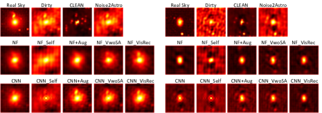
Figure 3: Visual Examples of overall comparison. VwoSA denotes VisRec w/o Sup-Aug.

4.3 Overall Comparison

To assess the performance of our method in scenarios with limited label availability, we conduct an overall comparison using only 1,024 labeled visibility examples ($|\mathcal{D}^{(s)}|=1,024$) and a set of 15,668 unlabeled data ($|\mathcal{D}^{(u)}|$ = 15,668). We calculate the LFD, PSNR, and SSIM values for all test data reconstructed using our method and other baseline methods, presenting both mean values and standard deviations in Table 1. The results show that both NF model Wu et al. (2022) and CNN model Schmidt et al. (2022) trained by supervised methods outperform traditional non-learning method (CLEAN) and self-supervised Noise2Astro Zhang et al. (2022). Our VisRec approach, applied to both neural field and CNN models, shows significant improvements in all metrics compared to the original supervised methods. Its variant model Supervised + Aug and VisRec w/o Sup-Aug also shows better reconstruction quality than the supervised versions, demonstrating that both the augmentation and the consistency training in VisRec are effective. We also present two sets of representative reconstructed images from EHT dataset in Figure 3.

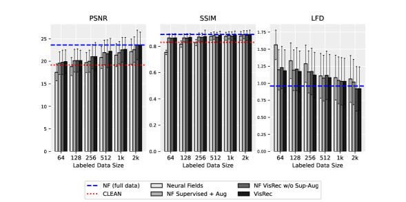
Figure 4: Effect of Labeled Data Size.

4.4 Effect of Labeled Data Size

We also evaluate the performance of our method and other baselines under various labeled data sizes. We apply VisRec, along with its two variants (Supervised + Aug and VisRec w/o Sup-Aug) to train the NF model Wu et al. (2022) on the EHT dataset. Maintaining a constant total training data size $|\mathcal{D}|$ = 16,692, we vary the size of the labeled subset $|\mathcal{D}^{(s)}|$ from 64 to 2k (k = 1024) and use the remaining data as the unlabeled subset. We also evaluate the performance of the original supervised model trained with all 16,692 labeled data examples, denoted NF (Full data). As shown in Figure 4, our method and its variants consistently outperform the original supervised method. With only 64 labeled examples, our method outperforms the traditional non-learning method CLEAN. With only 2k labeled examples, VisRec performs on par with supervised methods trained with over 16k examples. The results show that the effectiveness of VisRec comes from the use of both supervised and unsupervised data, making it well-suited for limited label scenarios. Moreover, incorporating data augmentation also improves model performance by enhancing training diversity.

In addition, we report the effect of labeled data size on VisRec performance with the CNN model in the appendix.

4.5 Robustness Evaluation

In this experiment, we evaluate the robustness of our method and the baselines under the same dataset setting as in section 4.3.

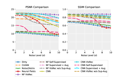
Figure 5: Performance of different methods across various noise levels. We only show PSNR and SSIM values because LFD is not applicable to Dirty, CLEAN, and Noise2Astro.

Robustness against Noise. In radio astronomy, both instrumental and environmental factors can introduce noise Schmidt et al. (2022), which may significantly degrade the quality of the images reconstructed by previous supervised learning methods. To evaluate the robustness of various methods to such noise, we conduct performance tests across different noise levels.

Following Schmidt et al. Schmidt et al. (2022), we add white noise that simulates potential measurement effects in the frequency domain by corrupting the visibilities with the noise of Gaussian distribution. This process can be represented as:

$$V_{\text{noisy}}(u_{s},v_{s})=V(u_{s},v_{s})+g(x|\mu,\sigma)_{uv}$$ (13)

where $g(x|\mu,\sigma)_{uv}$ is a random value generated for each frequency sample, with $\mu=0$ and noise level $\sigma=0\text{ to }10$. Figure 5 shows that models applied VisRec consistently outperform other methods and have lower sensitivity to noise. The two variant of our method (Supervised + Aug and VisRec w/o Sup-Aug) also show better robustness then the original supervised methods. We also display some visual examples in Figure 6, showing that as the noise level increases, the reconstruction of supervised learning methods are severely corrupted, whereas the reconstruction results of VisRec still maintain high quality.

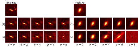
Figure 6: Visual examples of the effect of noise. Row (1) is the results of the NF model trained by VisRec and row (2) is the results of original supervised NF method. The examples are all from the EHT dataset.

Robustness against Missing Visibility Points. Missing visibility points, often resulting from offline antennas in interferometric arrays Nasirudin et al. (2022), also cause performance decrease of learning-based reconstruction methods. We vary the sample loss rate from 0 to 50% and evaluate the performance of our method and the baseline methods. Figure 7 shows that VisRec achieves the best overall sample loss rate and is less sensitive to increasing of missing samples than supervised methods. To show the result more clearly, we list the value of the NF model and CNN model trained with VisRec and the supervised method respectively in Table 2. The rate of VisRec performance decrease is significantly lower than supervised learning when applied to both NF and CNN models, indicating that VisRec improves the robustness of deep models.

Table 2: PSNR/SSIM values of methods at 0 and 50% sample loss rates.

Loss Rate	NF Sup	NF VisRec	CNN Sup	CNN VisRec
0	21.36 / 0.8754	22.63 / 0.8855	22.22 / 0.8636	23.37 / 0.8920
50%	19.25 / 0.8506	22.40 / 0.8848	19.59 / 0.8372	22.51 / 0.8889
Decrease	-9.88% / -2.83%	-1.02% / -0.08%	-11.84% / -3.06%	-3.68% / -0.35%

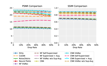
Figure 7: Performance of different methods across various sample loss rates. We only show PSNR and SSIM values because LFD is not applicable to Dirty, CLEAN, and Noise2Astro.

Table 3: Performance of training methods with the same or different datasets. Gray rows denote our method and its variants, and the rows in white background represent methods from prior studies.

Model	Same Dataset			Different Dataset
	LFD	SSIM	PSNR	LFD	SSIM	PSNR
Neural Field Wu et al. (2022)	1.083	0.875	21.36	1.319	0.819	16.74
NF Supervised + Aug	1.043	0.883	21.89	1.305	0.842	18.95
NF Self-Supervised	1.465	0.703	11.45	1.489	0.595	9.55
NF VisRec w/o Sup-Aug	1.029	0.877	22.53	1.242	0.844	18.42
NF VisRec	1.029	0.886	22.63	1.250	0.855	18.65
CNN Wu et al. (2022)	1.061	0.864	22.22	1.141	0.802	16.13
CNN Supervised + Aug	0.991	0.870	22.32	1.238	0.823	18.28
CNN Self-Supervised	1.481	0.785	15.17	1.409	0.736	11.88
CNN VisRec w/o Sup-Aug	0.897	0.873	22.60	1.044	0.822	16.99
CNN VisRec	0.950	0.892	23.37	1.001	0.866	20.65

4.6 Generalization to Another Telescope

We evaluate the generalizability of different methods by training the models on the EHT dataset (the same training setting as in Section 4.3) and testing their performance on both EHT and VLBA datasets. As shown in Table 3, the significant performance drop in all models when applied to different datasets underscores the challenge in model generalization. VisRec, VisRec w/o Sup-Aug, and Supervised+Aug methods outperform the traditional supervised method, especially on different datasets, indicating superior generalizability. While in some cases the variants of our method, e.g., VisRec w/o Sup-Aug, and Supervised+Aug show marginally better performance than VisRec in certain metrics, the overall performance of VisRec is superior. Particularly, the CNN model trained with VisRec shows the least performance degradation, suggesting its high generalizability in handling diverse data distributions.

4.7 Impact of Consistency Loss Weight

We evaluate the impact of consistency loss weight $\lambda$ in VisRec on the reconstruction of visibilities with different noise corruption levels. The results are shown in Figure 8. The performance of VisRec does not change much for a large range of $\lambda\in\left[0.01,0.8\right)$. Insensitivity to changes in $\lambda$ may help eliminate the need for hyperparameter tuning, which can simplify network training Desai et al. (2023).

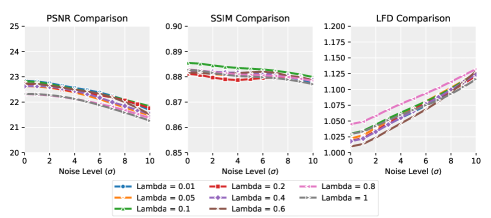
Figure 8: Impact of $\lambda$. The differences are small so we have narrowed the range of the y-axis for close observation.

5 Conclusion

In this study, we present VisRec, a semi-supervised learning framework for radio interferometric data reconstruction. VisRec effectively leverages both labeled and unlabeled data, significantly reducing dependence on extensive ground truth labels. Our results show that VisRec outperforms state-of-the-art methods in reconstruction quality, robustness to common observational perturbations, and generalizability across different telescope configurations.

References

- Blum et al. [2016] Robert D Blum, Kaylan Burleigh, Arjun Dey, David J Schlegel, Aaron M Meisner, Michael Levi, Adam D Myers, Dustin Lang, John Moustakas, Anna Patej, et al. The decam legacy survey. In American Astronomical Society Meeting Abstracts# 228, volume 228, pages 317–01, 2016.
- Bouman et al. [2016] Katherine L Bouman, Michael D Johnson, Daniel Zoran, Vincent L Fish, Sheperd S Doeleman, and William T Freeman. Computational imaging for vlbi image reconstruction. In Proceedings of the IEEE Conference on Computer Vision and Pattern Recognition, pages 913–922, 2016.
- Bouman et al. [2018] Katherine L Bouman, Michael D Johnson, Adrian V Dalca, Andrew A Chael, Freek Roelofs, Sheperd S Doeleman, and William T Freeman. Reconstructing video of time-varying sources from radio interferometric measurements. IEEE Transactions on Computational Imaging, 4(4):512–527, 2018.
- Chael et al. [2018] Andrew A Chael, Michael D Johnson, Katherine L Bouman, Lindy L Blackburn, Kazunori Akiyama, and Ramesh Narayan. Interferometric imaging directly with closure phases and closure amplitudes. The Astrophysical Journal, 857(1):23, 2018.
- Chael et al. [2019] Andrew A Chael, Katherine L Bouman, Michael D Johnson, Ramesh Narayan, Sheperd S Doeleman, John FC Wardle, Lindy L Blackburn, Kazunori Akiyama, Maciek Wielgus, Chi-kwan Chan, et al. ehtim: Imaging, analysis, and simulation software for radio interferometry. Astrophysics Source Code Library, pages ascl–1904, 2019.
- Connor et al. [2022] Liam Connor, Katherine L Bouman, Vikram Ravi, and Gregg Hallinan. Deep radio-interferometric imaging with polish: Dsa-2000 and weak lensing. Monthly Notices of the Royal Astronomical Society, 514(2):2614–2626, 2022.
- Dagli [2023] Rishit Dagli. Astroformer: More data might not be all you need for classification. arXiv preprint arXiv:2304.05350, 2023.
- Darestani et al. [2021] Mohammad Zalbagi Darestani, Akshay S Chaudhari, and Reinhard Heckel. Measuring robustness in deep learning based compressive sensing. In International Conference on Machine Learning, pages 2433–2444. PMLR, 2021.
- Desai et al. [2023] Arjun D Desai, Batu M Ozturkler, Christopher M Sandino, Robert Boutin, Marc Willis, Shreyas Vasanawala, Brian A Hargreaves, Christopher Ré, John M Pauly, and Akshay S Chaudhari. Noise2recon: Enabling snr-robust mri reconstruction with semi-supervised and self-supervised learning. Magnetic Resonance in Medicine, 90(5):2052–2070, 2023.
- Dey et al. [2019] Arjun Dey, David J Schlegel, Dustin Lang, Robert Blum, Kaylan Burleigh, Xiaohui Fan, Joseph R Findlay, Doug Finkbeiner, David Herrera, Stéphanie Juneau, et al. Overview of the desi legacy imaging surveys. The Astronomical Journal, 157(5):168, 2019.
- Geyer et al. [2023] F Geyer, K Schmidt, J Kummer, M Brüggen, HW Edler, D Elsässer, F Griese, A Poggenpohl, L Rustige, and W Rhode. Deep-learning-based radiointerferometric imaging with gan-aided training. Astronomy & Astrophysics, 677:A167, 2023.
- Henry [2021] Leung Henry. Galaxy10 decals dataset. https://github.com/henrysky/Galaxy10, 2021.
- Högbom [1974] JA Högbom. Aperture synthesis with a non-regular distribution of interferometer baselines. Astronomy and Astrophysics Supplement Series, 15:417, 1974.
- Jia et al. [2022] Jinghan Jia, Mingyi Hong, Yimeng Zhang, Mehmet Akcakaya, and Sijia Liu. On the robustness of deep learning-based mri reconstruction to image transformations. In Workshop on Trustworthy and Socially Responsible Machine Learning, NeurIPS 2022, 2022.
- Jiang et al. [2021] Liming Jiang, Bo Dai, Wayne Wu, and Chen Change Loy. Focal frequency loss for image reconstruction and synthesis. In Proceedings of the IEEE/CVF International Conference on Computer Vision, pages 13919–13929, 2021.
- Lehtinen et al. [2018] Jaakko Lehtinen, Jacob Munkberg, Jon Hasselgren, Samuli Laine, Tero Karras, Miika Aittala, and Timo Aila. Noise2noise: Learning image restoration without clean data. In International Conference on Machine Learning, pages 2965–2974. PMLR, 2018.
- Nasirudin et al. [2022] Ainulnabilah Nasirudin, David Prelogovic, Steven G Murray, Andrei Mesinger, and Gianni Bernardi. Characterizing beam errors for radio interferometric observations of reionization. Monthly Notices of the Royal Astronomical Society, 514(3):4655–4668, 2022.
- Paszke et al. [2019] Adam Paszke, Sam Gross, Francisco Massa, Adam Lerer, James Bradbury, Gregory Chanan, Trevor Killeen, Zeming Lin, Natalia Gimelshein, Luca Antiga, et al. Pytorch: An imperative style, high-performance deep learning library. Advances in neural information processing systems, 32, 2019.
- Schmidt et al. [2022] Kevin Schmidt, Felix Geyer, Stefan Fröse, Paul-Simon Blomenkamp, Marcus Brüggen, Francesco de Gasperin, Dominik Elsässer, and Wolfgang Rhode. Deep learning-based imaging in radio interferometry. arXiv preprint arXiv:2203.11757, 2022.
- Silva et al. [2016] David R Silva, Robert D Blum, Lori Allen, Arjun Dey, David J Schlegel, Dustin Lang, John Moustakas, Aaron M Meisner, Francisco Valdes, Anna Patej, et al. The mayall z-band legacy survey. In American Astronomical Society Meeting Abstracts# 228, volume 228, pages 317–02, 2016.
- Singh and Singh [2019] Himanshu Singh and Himanshu Singh. Basics of python and scikit image. Practical Machine Learning and Image Processing: For Facial Recognition, Object Detection, and Pattern Recognition Using Python, pages 29–61, 2019.
- Sun and Bouman [2021] He Sun and Katherine L Bouman. Deep probabilistic imaging: Uncertainty quantification and multi-modal solution characterization for computational imaging. In Proceedings of the AAAI Conference on Artificial Intelligence, volume 35, pages 2628–2637, 2021.
- Thompson et al. [2017] A Richard Thompson, James M Moran, and George W Swenson. Interferometry and synthesis in radio astronomy. Springer Nature, 2017.
- Wang et al. [2023] Ruoqi Wang, Zhuoyang Chen, Qiong Luo, and Feng Wang. A conditional denoising diffusion probabilistic model for radio interferometric image reconstruction. In 26th European Conference on Artificial Intelligence, pages 2499–2506, 2023.
- Wu et al. [2022] Benjamin Wu, Chao Liu, Benjamin Eckart, and Jan Kautz. Neural interferometry: Image reconstruction from astronomical interferometers using transformer-conditioned neural fields. In Proceedings of the AAAI Conference on Artificial Intelligence, 2022.
- Xu et al. [2023] Mingle Xu, Sook Yoon, Alvaro Fuentes, and Dong Sun Park. A comprehensive survey of image augmentation techniques for deep learning. Pattern Recognition, page 109347, 2023.
- Zhang et al. [2022] Yunchong Zhang, Brian Nord, Amanda Pagul, and Michael Lepori. Noise2astro: Astronomical image denoising with self-supervised neural networks. Research Notes of the AAS, 6(9):187, 2022.
- Zou et al. [2017] Hu Zou, Xu Zhou, Xiaohui Fan, Tianmeng Zhang, Zhimin Zhou, Jundan Nie, Xiyan Peng, Ian McGreer, Linhua Jiang, Arjun Dey, et al. Project overview of the beijing–arizona sky survey. Publications of the Astronomical Society of the Pacific, 129(976):064101, 2017.