Enhancing Multivariate Time Series Forecasting with Mutual Information-driven Cross-Variable and Temporal Modeling

Abstract

Recent advancements have underscored the impact of deep learning techniques on multivariate time series forecasting (MTSF). Generally, these techniques are bifurcated into two categories: Channel-independence and Channel-mixing approaches. Although Channel-independence methods typically yield better results, Channel-mixing could theoretically offer improvements by leveraging inter-variable correlations. Nonetheless, we argue that the integration of uncorrelated information in channel-mixing methods could curtail the potential enhancement in MTSF model performance. To substantiate this claim, we introduce the Cross-variable Decorrelation Aware feature Modeling (CDAM) for Channel-mixing approaches, aiming to refine Channel-mixing by minimizing redundant information between channels while enhancing relevant mutual information. Furthermore, we introduce the Temporal correlation Aware Modeling (TAM) to exploit temporal correlations, a step beyond conventional single-step forecasting methods. This strategy maximizes the mutual information between adjacent sub-sequences of both the forecasted and target series. Combining CDAM  and TAM, our novel framework significantly surpasses existing models, including those previously considered state-of-the-art, in comprehensive tests.

1 Introduction

Multivariate time series forecasting (MTSF) plays a pivotal role in diverse applications ranging from traffic flow estimation (Bai et al., 2020), weather prediction (Chen et al., 2021), energy consumption (Zhou et al., 2021) and healthcare (Bahadori & Lipton, 2019). Deep learning has ushered in a new era for MTSF, with methodologies rooted in RNN-based (Franceschi et al., 2019; Liu et al., 2018; Salinas et al., 2020; Rangapuram et al., 2018) and CNN-based models (Lea et al., 2017; Lai et al., 2018), that surpass the performance metrics set by traditional techniques (Box et al., 2015). A notable breakthrough has been the advent of Transformer-based models (Li et al., 2019; Zhou et al., 2021; Chen et al., 2021; Zhou et al., 2022). Equipped with attention mechanisms, these models adeptly seize long-range temporal dependencies, establishing a new benchmark for forecasting efficacy. While their primary intent is to harness multivariate correlations, recent research indicates a potential shortcoming: these models might not sufficiently discern cross-variable dependencies (Murphy & Chen, 2022; Nie et al., 2022; Zeng et al., 2022). This has spurred initiatives to tease out single variable information for more nuanced forecasting.

When it comes to modeling variable dependencies, MTSF models can be broadly classified into two categories: Channel-mixing models and Channel-independence models, as highlighted in Figure 1 (a) (Nie et al., 2022). Specifically, Channel-mixing models ingest all features from the time series, projecting them into an embedding space to blend information. Conversely, Channel-independence models restrict their input token to information sourced from just one channel. Recent studies (Murphy & Chen, 2022; Nie et al., 2022; Zeng et al., 2022) indicates that Channel-independence models significantly outpace Channel-mixing models on certain datasets. Yet, this advantage comes with a trade-off: the omission of crucial cross-variable information. Such an omission can be detrimental, especially when the variables inherently correlate. Illustratively, Figure 1 (b) showcases traffic flow variations from six proximate detectors in the PEMS08 dataset (Chen et al., 2001) . A discernible trend emerges across these detectors, suggesting that exploiting their interrelated patterns could bolster predictive accuracy for future traffic flows. In a comparative experiment, we trained both a Channel-independence model (PatchTST) and a Channel-mixing model (Informer) using the PEMS08 dataset. The outcome, as visualized in Figure 1 (c), unequivocally shows Informer’s superior performance over PatchTST, underscoring the importance of cross-variable insights. Motivated by these findings, we introduce the Cross-Variable Decorrelation Aware Feature Modeling (CDAM) for Channel-mixing methodologies. CDAM  aims to hone in on cross-variable information and prune redundant data. It achieves this by minimizing mutual information between the latent depiction of an individual univariate time series and related multivariate inputs, while concurrently amplifying the shared mutual information between the latent model, its univariate input, and the subsequent univariate forecast.

Apart from modeling channel dependence, another significant challenge in MTSF is the accumulation of errors along time, as shown in Figure 1 (a). To mitigate this, a number of studies (Nie et al., 2022; Zeng et al., 2022; Zhou et al., 2021; Zhang & Yan, ) have adopted a direct forecasting strategy using a single-step forecaster that generates multi-step predictions in a single step, typically configured as a fully-connected network. Although often superior to auto-regressive forecasters, this method tends to neglect the temporal correlations across varied timesteps in the target series, curtailing its potential to capture series inter-dependencies effectively. Drawing inspiration from the notable temporal relationships observed in adjacent sub-sequences post-downsampling (Liu et al., 2022a), we propose Temporal Correlation Aware Modeling (TAM), which iteratively down-samples and optimizes mutual information between consecutive sub-sequences of both the forecasted and target series.

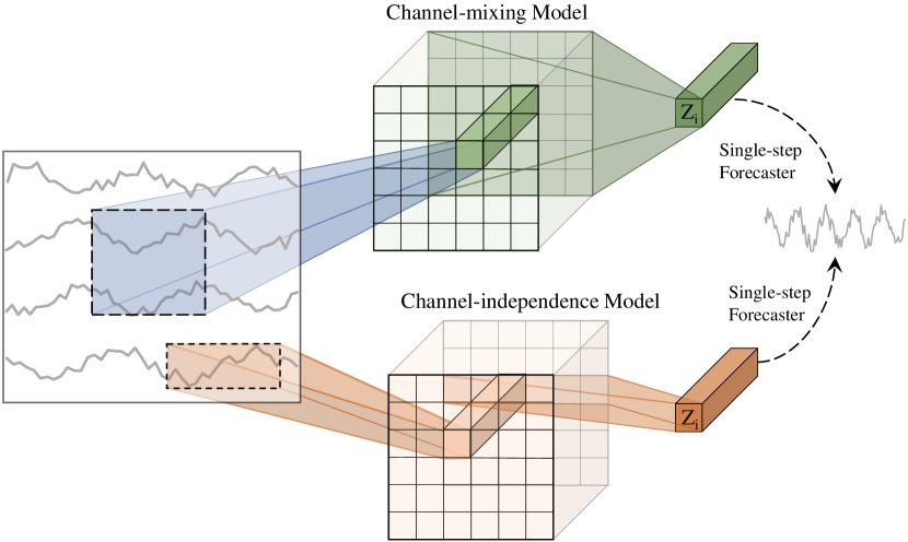
(a) The Framework of Channel-Independence and Channel-mixing models

(b) Traffic flow of 5 adjacent detectors in PEMS08

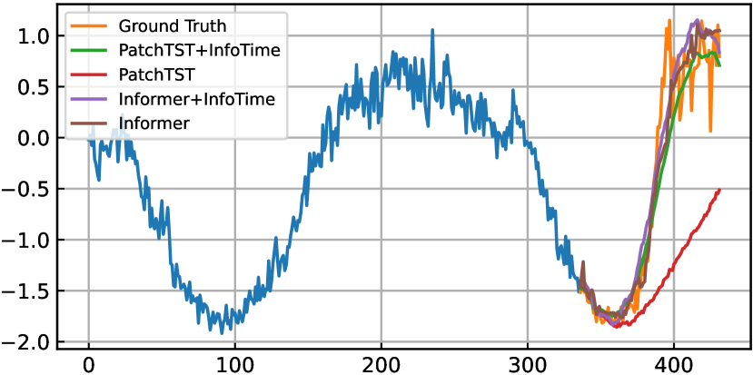
(c) Prediction results of PatchTST and Informer in PEMS08

Figure 1: (a) The framework of Channel-independence models and Channel-mixing models. Given historical series $X=\{X^{i}\}$ where $i$ denotes the channel index, the Channel-mixing model tends to maximize the mutual information between $X$ and the latent representation $Z^{i}$. Additionally, it maximize the mutual information between $Z^{i}$ and the i-th future series $Y^{i}$. The Channel-independence models maximize the mutual information between the i-th historical series $X^{i}$ and $Z^{i}$ while ignoring the mutual information between $Z^{i}$ and other channels; (b) Traffic flow of 5 adjacent detectors in the PEMS08 dataset; and (c) Prediction results of Channel-independence model (PatchTST), Channel-mixing model (Informer), and that with our framework, respectively.

In essence, this paper delves into two pivotal challenges in multivariate time series forecasting: cross-variable relationships and temporal relationships. Drawing inspiration from these challenges, we develop a novel framework, denoted as InfoTime. This framework seamlessly integrates CDAM and TAM. Our paper’s key contributions encompass:

• We introduce Cross-Variable Decorrelation Aware Feature Modeling (CDAM) designed specifically for Channel-mixing methods. It adeptly distills cross-variable information, simultaneously filtering out superfluous information.

• Our proposed Temporal Correlation Aware Modeling (TAM) is tailored to effectively capture the temporal correlations across varied timesteps in the target series.

• Synthesizing CDAM and TAM, we unveil a cutting-edge framework for MTSF, denominated as InfoTime.

Through rigorous experimentation on diverse real-world datasets, it’s evident that our InfoTime consistently eclipses existing Channel-mixing benchmarks, achieving superior accuracy and notably mitigating overfitting. Furthermore, InfoTime enhances the efficacy of Channel-Independent models, especially in instances with ambiguous cross-variable traits.

2 Related Work

2.1 Multivariate Time Series Forecasting

Multivariate time series forecasting is the task of predicting future values of variables, given historical observations. With the development of deep learning, various neural models have been proposed and demonstrated promising performance in this task. RNN-based (Franceschi et al., 2019; Salinas et al., 2020; Rangapuram et al., 2018) and CNN-based (Lea et al., 2017; Lai et al., 2018) models are proposed for models time series data using RNN or CNN respectively, but these models have difficulty in modeling long-term dependency. In recent years, a large body of works try to apply Transformer models to forecast long-term multivariate series and have shown great potential (Li et al., 2019; Zhou et al., 2021; Chen et al., 2021; Zhou et al., 2022; Nie et al., 2022), Especially, LogTrans (Li et al., 2019) proposes the LogSparse attention in order to reduce the complexity from $O(L^{2})$ to $O(L(\log L)^{2})$. Informer (Zhou et al., 2021) utilizes the sparsity of attention score through KL-divergence estimation and proposes ProbSparse self-attention mechanism which achieves $O(L\log L)$ complexity. Autoformer (Chen et al., 2021) introduces a decomposition architecture with the Auto-Correlation mechanism to capture the seasonal and trend features of historical series which also achieves $O(L\log L)$ complexity and has a better performance. Afterword, FEDformer (Zhou et al., 2022) employs the mixture-of-expert to enhance the seasonal-trend decomposition and achieves $O(L)$ complexity. The above methods focus on modeling temporal dependency yet omit the correlation of different variables. Crossformer (Zhang & Yan, ) introduces Two-Stage Attention to effectively capture the cross-time and cross-dimension dependency. But the effectiveness of Crossformer is limited. Recently, several works (Murphy & Chen, 2022; Nie et al., 2022; Zeng et al., 2022) observe that modeling cross-dimension dependency makes neural models suffer from overfitting in most benchmarks, therefore, they propose Channel-Independence methods to avoid this issue. However, the improvement is based on the sacrifice of cross-variable information. Besides, existing models primarily focus on extracting correlations of historical series while disregarding the correlations of target series.

2.2 Mutual Information and Information Bottleneck

Mutual Information (MI) is an entropy-based measure that quantifies the dependence between random variables which has the form:

$$I(X;Y)=\int p(x,y)log\frac{p(x,y)}{p(x)p(y)}dxdy$$ (1)

Mutual Information was used in a wide range of domains and tasks, including feature selection (Kwak & Choi, 2002), causality (Butte & Kohane, 1999), and Information Bottleneck (Tishby et al., 2000). Information Bottleneck (IB) was first proposed by (Tishby et al., 2000) which is an information theoretic framework for extracting the most relevant information in the relationship of the input with respect to the output, which can be formulated as $max\,\,I(Y;Z)-\beta I(X;Z)$. Several works (Tishby & Zaslavsky, 2015; Shwartz-Ziv & Tishby, 2017) try to use the Information Bottleneck framework to analyze the Deep Neural Networks by quantifying Mutual Information between the network layers and deriving an information theoretic limit on DNN efficiency. Variational Information Bottleneck (VIB) was also proposed (Alemi et al., 2016) to bridge the gap between Information Bottleneck and deep learning. In recent years, many lower-bound estimations (Belghazi et al., 2018; Oord et al., 2018) and upper-bound estimations (Poole et al., 2019; Cheng et al., 2020) have been proposed to estimate MI effectively which are useful to estimate VIB. Nowadays, MI and VIB have been widely used in computer vision (Schulz et al., 2020; Luo et al., 2019), natural language processing (Mahabadi et al., 2021; West et al., 2019; Voita et al., 2019), reinforcement learning (Goyal et al., 2019; Igl et al., 2019), and representation learning (Federici et al., 2020; Hjelm et al., 2018). However, Mutual Information and Information Bottleneck are less researched in long-term multivariate time-series forecasting.

3 Method

In multivariate time series forecasting, one aims to predict the future value of time series $y_{t}=s_{t+T+1:t+T+P}\in\mathbb{R}^{P\times C}$ given the history $x_{t}=s_{t:t+T}\in\mathbb{R}^{T\times C}$, where $T$ and $P$ refer the number of time steps in the past and future. $C\geq 1$ refers the number of variables. Given time series $s$, we divide it into history set $X=\{x_{1},...,x_{N}\}$ and future set $Y=\{y_{1},...,y_{N}\}$, where $N$ is the number of samples. As depicted in Figure 1 (a), deep learning methods first extract latent representation $Z^{i}$ from $X$ (Channel-mixing) , or $X^{i}$ (Channel-independence) , and subsequently generate target series $Y^{i}$ from $Z^{i}$. A natural assumption is that these $C$ series are associated which helps to improve the forecasting accuracy. To leverage the cross-variable dependencies while eliminating superfluous information, in Section 3.1, we propose the Cross-Variable Decorrelation Aware Feature Modeling (CDAM) to extract cross-variable dependencies. Additionally, in section 3.2, we introduce Temporal Aware Modeling (TAM) that explicitly models the correlation of predicted series and allows to generate more accurate predictions compared to the single-step forecaster.

3.1 Cross-Variable Decorrelation Aware Feature Modeling

Recent studies (Nie et al., 2022; Zeng et al., 2022; Zhou et al., 2021; Zhang & Yan, ) have demonstrated that Channel-independence is more effective in achieving high-level performance than Channel-mixing. However, it is important to note that multivariate time series inherently contain correlations among variables. Channel-mixing aims to leverage these cross-variable dependencies for predicting future series, but it often fails to improve the performance of MTSF. One possible reason for this is that Channel-mixing introduces superfluous information. To verify this, we introduce CDAM to extract cross-variable information while eliminating superfluous information. Specifically, drawing inspiration from information bottlenecks, CDAM maximizes the joint mutual information among the latent representation $Z^{i}$, its univariate input $X^{i}$ and the corresponding univariate target series $Y^{i}$. Simultaneously, it minimizes the mutual information between latent representation $Z^{i}$ of one single univariate time series and other multivariate series input $X^{o}$. This leads us to formulate the following objective:

$$\max\,\,I(Y^{i},X^{i};Z^{i})\,\,s.t.\,\,I(X^{o};Z^{i})\leq{I_{c}},$$ (2)

where $I(Y^{i},X^{i};Z^{i})$ represents the joint mutual information between the target series $Y^{i}$, the univariate input $X^{i}$, and the latent representation $Z^{i}$. Additionally, $I(X^{o};Z^{i})$ represents the mutual information between the latent representation $Z^{i}$ and the other multivariate input series $X^{o}$. The constraint $I(X^{o};Z^{i})\leq I_{c}$ ensures that the mutual information between $X^{o}$ and $Z^{i}$ is limited to a predefined threshold $I_{c}$.

With the introduction of a Lagrange multiplier $\beta$, we can maximize the objective function for the i-th channel as follows:

$$\mathcal{R}_{IB}^{i} =I(Y^{i},X^{i};Z^{i})-\beta I(X^{o};Z^{i})$$ (3)

$$=I(Y^{i};Z^{i}|X^{i})+I(X^{i};Z^{i})-\beta I(X^{o};Z^{i}),$$

where $\beta\geq 0$ controls the tradeoff between $I(Y^{i};Z^{i}|X^{i})$, $I(X^{i};Z^{i})$ and $I(X^{o};Z^{i})$, the larger $\beta$ corresponds to lower mutual information between $X^{o}$ and $Z^{i}$, indicating that $Z^{i}$ needs to retain important information from $X^{o}$ while eliminating irrelevant information to ensure accurate prediction of $Y^{i}$. However, the computation of mutual information $I(X^{i},Y^{i};Z^{i})$ and $I(X^{o};Z^{i})$ is intractable. Therefore, we provide variational lower bounds and upper bounds for $I(X^{i},Y^{i};Z^{i})$ and $I(X^{o};Z^{i})$, respectively.

Lower bound for $I(X^{i},Y^{i};Z^{i})$. The joint mutual information between latent representation $Z^{i}$, i-th historical series $X^{i}$, and i-th target series $Y^{i}$ is defined as (More details are shown in Appendix A.4.1):

$$I(X^{i},Y^{i};Z^{i}) =I(Z^{i};X^{i})+I(Z^{i};Y^{i}|X^{i})$$ (4)

$$=\mathbb{E}_{p(z^{i},y^{i},x^{i})}\left[\log p(y^{i}|x^{i},z^{i})\right]$$

$$+\mathbb{E}_{p(z^{i},x^{i})}\left[\log p(x^{i}|z^{i})\right]+H(Y^{i},X^{i}),$$

where the joint entropy $H(Y^{i},X^{i})=-\int p(y^{i},x^{i})dx^{i}dy^{i}$ is only related to the dataset and cannot be optimized, so can be ignored. Therefore, the MI can be simplified as:

$$I(X^{i},Y^{i};Z^{i}) =\mathbb{E}_{p(z^{i},y^{i},x^{i})}\left[\log p(y^{i}|x^{i},z^{i})\right]$$ (5)

$$+\mathbb{E}_{p(z^{i},x^{i})}\left[\log p(x^{i}|z^{i})\right]+\text{constant}.$$

Since $p(y^{i}|x^{i},z^{i})$ and $p(x^{i}|z^{i})$ are intractable, we introduce $p_{\theta}(y^{i}|z^{i},x^{i})$ and $p_{\theta}(x^{i}|z^{i})$ to be the variational approximation to $p(y^{i}|x^{i},z^{i})$ and $p(x^{i}|z^{i})$, respectively. Thus the variational lower bound can be expressed as (More details are shown in Appendix A.4.2):

$$I(X^{i},Y^{i};Z^{i})-\text{constant} \geq\mathbb{E}_{p(z^{i},y^{i},x^{i})}\left[\log p_{\theta}(y^{i}|x^{i},z^{i})\right]$$

$$+\mathbb{E}_{p(z^{i},x^{i})}\left[\log p_{\theta}(x^{i}|z^{i})\right]$$

$$=I_{v}(X^{i},Y^{i};Z^{i}).$$ (6)

Hence, the maximization of $I(X^{i},Y^{i};Z^{i})$ can be achieved by maximizing $I_{v}(X^{i},Y^{i};Z^{i})$. We assume the variational distribution $p_{\theta}(y^{i}|z^{i},x^{i})$ and $p_{\theta}(x^{i}|z^{i})$ as the Gaussion distribution. Consequently, the first term of $I_{v}(X^{i},Y^{i};Z^{i})$ represents the negative log-likelihood of predicting $Y^{i}$ given $Z^{i}$ and $X^{i}$, while the second term aims to reconstruct $X^{i}$ given $Z^{i}$.

Upper bound for $I(X^{o};Z^{i})$. Next, to minimize the MI between the latent representation $Z^{i}$ and historical series $X^{o}$, we adopt the sampled vCLUB as defined in (Cheng et al., 2020):

$$I_{v}(X^{o};Z^{i})=\frac{1}{N}\sum_{n=1}^{N}\left[\log q_{\theta}(z_{n}^{i}|x_{n}^{o})-\log q_{\theta}(z_{n}^{i}|x^{o}_{k^{\prime}_{n}})\right],$$ (7)

where $(z_{n}^{i},x^{o}_{k^{\prime}_{n}})$ represents a negative pair and $k_{n}^{\prime}$ is uniformly selected from indices $\{1,2,...N\}$. By minimizing $I_{v}(X^{o};Z^{i})$, we can effectively minimize $I(X^{o};Z^{i})$. It enables the model to extract relevant cross-variable information while eliminating irrelevant information.

Finally, We can convert the intractable objective function $\mathcal{R}_{IB}^{i}$ of all channels in Eq. 3 as:

$$\mathcal{L}_{IB} =\frac{1}{C}\sum_{i=1}^{C}\left[-I_{v}(X^{i},Y^{i};Z^{i})+\beta I_{v}(X^{o};Z^{i})\right]$$

$${\geq-\frac{1}{C}\sum_{i=1}^{C}\mathcal{R}_{IB}^{i}}=-\mathcal{R}_{IB}.$$

The objective function $\mathcal{L}_{IB}$ is a tractable approximation of the original objective function $\mathcal{R}_{IB}$, we can effectively maximize $\mathcal{R}_{IB}^{i}$ by minimizing $\mathcal{L}_{IB}$.

3.2 Temporal Correlation Aware Modeling

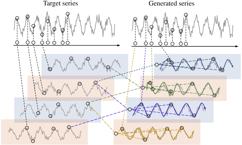
Figure 2: Architecture of TAM with 4$\times$ dowmsampling. We downsample the target series and forecasted series utilizing single-forecaster into four sub-sequences, respectively. And then we maximize the mutual information between the adjacent sub-sequences of forecasted series and target series.

Previous works (Nie et al., 2022; Zeng et al., 2022; Zhou et al., 2021; Zhang & Yan, ) have attempted to alleviate error accumulation effects by using a single-step forecaster, which is typically implemented as a fully-connected network, to predict future time series. Unlike auto-regressive forecasters, which consider dependencies between predicted future time steps, the single-step forecaster assumes that the predicted time steps are independent of each other given the historical time series. Consequently, the training objective of the single-step forecaster can be expressed as:

$$p(y^{i}|z^{i},x^{i})=\prod_{j=1}^{P}p(y^{i}_{j}|z^{i},x^{i})$$ (8)

While the single-step forecaster outperforms the auto-regressive forecaster, it falls short in capturing the temporal correlations among different timesteps in the target series. In contrast to NLP, time series data is considered a low-density information source (Lin et al., 2023). One unique property of time series data is that the temporal relations, such as trends and seasonality, are similar between downsampling adjacent sub-sequences (Liu et al., 2022a). Building upon the above observation, we propose TAM to enhance the correlation of predicted future time steps by iteratively down-sampling the time series and optimizing the mutual information between consecutive sub-sequences of both the forecasted and target series. Next, we will introduce TAM in detail.

After extracting cross-variable feature $Z^{i}$ as described in Sec 3.1, we first generate $\hat{Y^{i}}$ using a single-step forecaster that leverages the historical data of the i-th channel $X^{i}$ and $Z^{i}$ . The forecasted series $\hat{Y}$ and target series $Y$ are then downsampled $N$ times. For the n-th ($n\leq N$) downsampling, we generate $m$ sub-sequences $\hat{Y}=\{\hat{Y}_{1},...,\hat{Y}_{m}\}$,$Y=\{Y_{1},...,Y_{m}\}$, where $m=2^{n}$ and $\hat{Y}_{j}\in R^{\frac{P}{2^{n}}\times C}$. Next, we aim to maximize the mutual information $\hat{Y}_{j}^{i}$ and $Y_{j-1}^{i}$, $Y_{j+1}^{i}$, given $X^{i}$, where $1<j<m$. This is achieved by calculating $\mathcal{L}_{n}$ for the $n$-the downsampling:

$$\mathcal{L}_{n} =-\frac{1}{mC}\sum_{i=1}^{C}\Big{[}I(Y_{2}^{i};\hat{Y}_{1}^{i}|X^{i})+I(Y_{m-1}^{i};\hat{Y}_{m}^{i}|X^{i})$$

$$+\sum_{j=2}^{m-1}I(Y_{j-1}^{i};\hat{Y}_{j}^{i}|X^{i})+I(Y_{j+1}^{i};\hat{Y}_{j}^{i}|X^{i})\Big{]}.$$

We also introduce the variational lower bound for $I(Y^{i}_{j-1};\hat{Y}_{j}^{i}|X^{i})$, which is as follows (More details are shown in Appendix A.5):

$$I(Y^{i}_{j-1};\hat{Y}_{j}^{i}|X^{i})\geq\mathbb{E}_{p(y_{j-1}^{i},\hat{y}_{j}^{i},x^{i})}\left[p_{\theta}(y_{j-1}^{i}|\hat{y}_{j}^{i},x^{i})\right].$$ (9)

Furthermore, considering the efficiency, we make the assumption that the time steps of a sub-sequence are independent given the adjacent sub-sequence. As a result, we can simplify the mutual information term, $I(Y^{i}_{j-1};\hat{Y}_{j}^{i}|X^{i})$ as $I(Y^{i}_{j-1};\hat{Y}_{j}^{i}|X^{i})=\sum_{k=1}^{\frac{P}{2^{n}}}\left[I(Y^{i}_{j-1,k};\hat{Y}_{j}^{i}|X^{i})\right]$. This allows us to generate the entire sub-sequence in a single step without requiring auto-regression.

For the n-th downsampling, TAM will generate $2\times(2^{n}-1)$ sub-sequences denoted as $\hat{Y}^{\prime}=\{\hat{Y}_{1}^{r},\hat{Y}_{2}^{l},\hat{Y}_{2}^{r},...,\hat{Y}_{m}^{l}\}$. These sub-sequences, except for the ones and the ends, are predicted by their left and right adjacent sub-sequences respectively. We then splice these $2\times(2^{n}-1)$ sub-sequences into a new series $\hat{Y}_{n}=\{\hat{Y}_{1}^{r},\frac{\hat{Y}_{2}^{l}+\hat{Y}_{2}^{r}}{2},...,\hat{Y}_{m}^{l}\}$. After $N$ downsamplings, we have generated $N+1$ series. We use these $N+1$ series as the final forecasting results, resulting in the following loss function:

$$\mathcal{L}_{p}=||Y-(\lambda\sum_{n=1}^{N}{\frac{\hat{Y}_{n}}{N}}+(1-\lambda)\hat{Y})||_{2}^{2}$$ (10)

In contrast to single-step forecasters that generate multi-step predictions without considering the correlation between the predicted series, our proposed method, referred to as TAM, explicitly models the correlation of predicted future time steps and allows to generate more accurate and coherent predictions.

Integrating CDAM and TAM, the total loss of InfoTime can be written as :

$$\mathcal{L}_{total}=\mathcal{L}_{IB}+\sum_{n=1}^{N}\mathcal{L}_{n}+\mathcal{L}_{p}.$$ (11)

4 Experiments

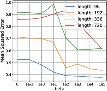
(a) Informer on ETTh1

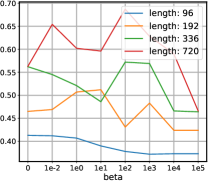
(b) Stationary on ETTh1

(c) PatchTST on ETTh1

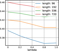
(d) RMLP on ETTh1

Figure 3: Evaluation on hyper-parameter $\beta$ and $\lambda$. We evaluate the impact of $\beta$ with Informer and Stationary on the ETTh1 dataset, we also evaluate $\lambda$ with PatchTST and RMLP on the ETTh1 dataset.

Table 1: Multivariate long-term series forecasting results on Channel-mixing models with different prediction lengths $O\in\{96,192,336,720\}$. We set the input length $I$ as 96 for all the models. The best result is indicated in bold font. Avg is averaged from all four prediction lengths. and Pro means the relative MSE or MAE reduction. (See Table LABEL:tab:ablation_dependent for the full results.)

Models		Informer				Stationary				Crossformer
		Original		w/Ours		Original		w/Ours		Original		w/Ours
Metric		MSE	MAE	MSE	MAE	MSE	MAE	MSE	MAE	MSE	MAE	MSE	MAE
ETTm2	96	0.365	0.453	0.187	0.282	0.201	0.291	0.175	0.256	0.281	0.373	0.186	0.281
	192	0.533	0.563	0.277	0.351	0.275	0.335	0.238	0.297	0.549	0.520	0.269	0.341
	336	1.363	0.887	0.380	0.420	0.350	0.377	0.299	0.336	0.729	0.603	0.356	0.396
	720	3.379	1.338	0.607	0.549	0.460	0.435	0.398	0.393	1.059	0.741	0.493	0.482
	Avg	1.410	0.810	0.362	0.400	0.321	0.359	0.277	0.320	0.654	0.559	0.326	0.375
	Pro	-	-	74.3%	50.6%	-	-	13.7%	10.8%	-	-	50.1%	32.9%
Weather	96	0.300	0.384	0.179	0.249	0.181	0.230	0.166	0.213	0.158	0.236	0.149	0.218
	192	0.598	0.544	0.226	0.296	0.286	0.312	0.218	0.260	0.209	0.285	0.202	0.272
	336	0.578	0.523	0.276	0.334	0.319	0.335	0.274	0.300	0.265	0.328	0.256	0.313
	720	1.059	0.741	0.332	0.372	0.411	0.393	0.351	0.353	0.376	0.397	0.329	0.366
	Avg	0.633	0.548	0.253	0.312	0.299	0.317	0.252	0.281	0.252	0.311	0.234	0.292
	Pro	-	-	60.0%	43.0%	-	-	15.7%	11.3%	-	-	7.1%	6.1%
Traffic	96	0.719	0.391	0.505	0.348	0.599	0.332	0.459	0.311	0.609	0.362	0.529	0.334
	192	0.696	0.379	0.521	0.354	0.619	0.341	0.475	0.315	0.623	0.365	0.519	0.327
	336	0.777	0.420	0.520	0.337	0.651	0.347	0.486	0.319	0.649	0.370	0.521	0.337
	720	0.864	0.472	0.552	0.352	0.658	0.358	0.522	0.338	0.758	0.418	0.556	0.350
	Avg	0.764	0.415	0.524	0.347	0.631	0.344	0.485	0.320	0.659	0.378	0.531	0.337
	Pro	-	-	31.4%	16.3%	-	-	23.1%	6.9%	-	-	19.4%	10.8%
Electricity	96	0.274	0.368	0.195	0.300	0.168	0.271	0.154	0.256	0.170	0.279	0.150	0.248
	192	0.296	0.386	0.193	0.291	0.186	0.285	0.163	0.263	0.198	0.303	0.168	0.263
	336	0.300	0.394	0.206	0.300	0.194	0.297	0.178	0.279	0.235	0.328	0.200	0.290
	720	0.373	0.439	0.241	0.332	0.224	0.316	0.201	0.299	0.270	0.360	0.235	0.323
	Avg	0.310	0.397	0.208	0.305	0.193	0.292	0.174	0.274	0.218	0.317	0.188	0.281
	Pro	-	-	32.9%	23.1%	-	-	9.8%	6.1%	-	-	13.7%	11.3%

In this section, we extensively evaluate the proposed InfoTime on 10 real-world benchmarks using various Channel-mixing and Channel-Independence models, including state-of-the-art models.

Baselines. In order to demonstrate the versatility of our proposed method, InfoTime, we evaluate it on various deep-learning-based forecasting models, including several popular baselines as well as the state-of-the-art method. For Channel-mixing models, we select Informer (Zhou et al., 2021), Non-stationary Transformer (Liu et al., 2022b), denoting as Stationary, and Crossformer (Zhang & Yan, ). As for Channel-Independence models, we utilize PatchTST (Nie et al., 2022) and also introduce RMLP which consists of two linear layers with ReLU activation and also incorporates reversible instance normalization (Kim et al., 2021). (see Appendix A.2 for more details)

Datasets. We extensively include 10 real world datasets in our experiments, including four ETT datasets (ETTh1, ETTh2, ETTm1, ETTm2) (Zhou et al., 2021). Electricity, Weather, Traffic (Chen et al., 2021), and PEMS covering energy, transportation and weather domains (See Appendix A.1 for more details on the datasets). We follow the standard protocol that divides each dataset into the training, validation, and testing subsets according to the chronological order. The split ratio is 6:2:2 for the ETT dataset and 7:1:2 for others.

4.1 Main Results

Table 1 compares the forecasting accuracy of the Channel-mixing baselines and InfoTime. The results clearly demonstrate that InfoTime consistently outperforms all three baselines, namely Informer, Stationary, and Crossformer, by a significant margin. This improvement is particularly notable for long sequence predictions, which are generally more challenging and prone to the model relying on irrelevant cross-variable information. InfoTime exhibits stable performance, whereas the baselines experience a substantial increase in forecasting error as the prediction length is extended. For example, on the ETTm2 dataset, when the prediction length increases from 96 to 720, the forecasting error of Informer rises significantly from 0.365 to 3.379. In contrast, InfoTime shows a much slight increase in error. A similar tendency appears with the other prediction lengths, datasets, and baseline models as well. These results demonstrate that InfoTime makes the baseline models more robust to prediction target series.

To gain further insights into why InfoTime outperforms baselines, we visualize the testing error for each epoch in Figure 4. Overall, InfoTime exhibits lower and more stable test errors compared to the baselines. Moreover, the baselines are highly prone to overfitting in the early stages of training, whereas InfoTime effectively mitigates this issue.

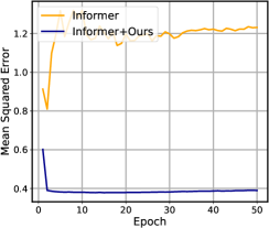
(a) Test error on Informer

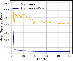
(b) Test error on Stationary

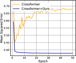
(c) Test error on Crossformer

Figure 4: Test error for each training epoch. We train the baselines and integrated with our InfoTime for 50 epochs on ETTh1 with the history and prediction length are both 96.

Table 2: Multivariate long-term series forecasting results on Channel-Independence models with different prediction lengths. We set the input length $I$ as 336 for all the models. The best result is indicated in bold font. See Table 6 in the Appendix for the full results.

Models		Metric	ETTh1				ETTm1				Traffic
			96	192	336	720	96	192	336	720	96	192	336	720
PatchTST	Original	MSE	0.375	0.414	0.440	0.460	0.290	0.332	0.366	0.420	0.367	0.385	0.398	0.434
		MAE	0.399	0.421	0.440	0.473	0.342	0.369	0.392	0.424	0.251	0.259	0.265	0.287
	w/Ours	MSE	0.365	0.403	0.427	0.433	0.283	0.322	0.356	0.407	0.358	0.379	0.391	0.425
		MAE	0.389	0.413	0.428	0.453	0.335	0.359	0.382	0.417	0.245	0.254	0.261	0.280
RMLP	Original	MSE	0.380	0.414	0.439	0.470	0.290	0.329	0.364	0.430	0.383	0.401	0.414	0.443
		MAE	0.401	0.421	0.436	0.471	0.343	0.368	0.390	0.426	0.269	0.276	0.282	0.309
	w/Ours	MSE	0.367	0.404	0.426	0.439	0.285	0.322	0.358	0.414	0.364	0.384	0.398	0.428
		MAE	0.391	0.413	0.429	0.459	0.335	0.359	0.381	0.413	0.249	0.258	0.266	0.284

We also present the forecasting results of Channel-independence baselines in Table 2. It is worth noting that InfoTime also surpasses Channel-independence baselines, indicating that although Channel-independence models exhibit promising results, incorporating cross-variable features can further enhance their effectiveness. Furthermore, we evaluate InfoTime on the PEMS datasets, which consist of variables that exhibit clear geographical correlations. The results in Table 3 reveal a significant performance gap between PatchTST and RMLP compared to Informer, suggesting that Channel-independence models may not be optimal in scenarios where there are clear correlations between variables. In contrast, our framework exhibits improved performance for both Channel-mixing and Channel-independence models.

Table 3: Multivariate long-term series forecasting results on baselines and PEMS datasets with different prediction lengths. We set the input length $I$ as 336 for all the models. The best result is indicated in bold font. (See Table 9 for the full results.)

Models		Metric	PEMS03				PEMS04				PEMS08
			96	192	336	720	96	192	336	720	96	192	336	720
PatchTST	Original	MSE	0.180	0.207	0.223	0.291	0.195	0.218	0.237	0.321	0.239	0.292	0.314	0.372
		MAE	0.281	0.295	0.309	0.364	0.296	0.314	0.329	0.394	0.324	0.351	0.374	0.425
	w/Ours	MSE	0.115	0.154	0.164	0.198	0.110	0.118	0.129	0.149	0.114	0.160	0.177	0.209
		MAE	0.223	0.251	0.256	0.286	0.221	0.224	0.237	0.261	0.218	0.243	0.241	0.281
RMLP	Original	MSE	0.160	0.184	0.201	0.254	0.175	0.199	0.210	0.255	0.194	0.251	0.274	0.306
		MAE	0.257	0.277	0.291	0.337	0.278	0.294	0.306	0.348	0.279	0.311	0.328	0.365
	w/Ours	MSE	0.117	0.159	0.146	0.204	0.103	0.114	0.130	0.154	0.116	0.156	0.175	0.181
		MAE	0.228	0.252	0.246	0.285	0.211	0.219	0.236	0.264	0.215	0.235	0.242	0.255

4.2 Ablation Study

Table 4: Component ablation of InfoTime. We set the input length $I$ as 336 for PatchTST and 96 for Informer. The best results are in bold and the second best are underlined. (See Table LABEL:tab:ablation_dependent and Table LABEL:tab:ablation_independent in the Appendix for the full ablation results.)

Models		Informer						PatchTST
		Original		+TAM		+InfoTime		Original		+TAM		+InfoTime
Metric		MSE	MAE	MSE	MAE	MSE	MAE	MSE	MAE	MSE	MAE	MSE	MAE
ETTm1	96	0.672	0.571	0.435	0.444	0.335	0.369	0.290	0.342	0.286	0.337	0.283	0.335
	192	0.795	0.669	0.473	0.467	0.380	0.390	0.332	0.369	0.326	0.366	0.322	0.363
	336	1.212	0.871	0.545	0.518	0.423	0.426	0.366	0.392	0.359	0.388	0.356	0.385
	720	1.166	0.823	0.669	0.589	0.505	0.480	0.420	0.424	0.408	0.413	0.407	0.417
Weather	96	0.300	0.384	0.277	0.354	0.179	0.249	0.152	0.199	0.149	0.197	0.144	0.194
	192	0.598	0.544	0.407	0.447	0.226	0.296	0.197	0.243	0.192	0.238	0.189	0.238
	336	0.578	0.523	0.529	0.520	0.276	0.334	0.250	0.284	0.247	0.280	0.239	0.279
	720	1.059	0.741	0.951	0.734	0.332	0.372	0.320	0.335	0.321	0.332	0.312	0.331

In our approach, there are two components: CDAM and TAM. To investigate the effectiveness of these components, we conduct an ablation study on the ETTm1 and Weather datasets with Informer and PatchTST. +TAM means that we add TAM to these baselines and +InfoTime means that we add both CDAM and TAM to baselines. The results of this ablation study are summarized in Table LABEL:tab:ablation. Compared to baselines using the single-step forecaster, TAM performs better in most settings, which indicates the importance of cross-time correlation. For Channel-mixing models, we find that InfoTime can significantly enhance their performance and effectively alleviate the issue of overfitting. For Channel-Independence models, InfoTime still improves their performance, which indicates that correctly establishing the dependency between variables is an effective way to improve performance.

4.3 Effect of Hyper-Parameters

We investigate the impact of the hyper-parameter $\beta$ on the ETTh1 and ETTm2 datasets with two baselines. In Figure 3 (a) (b), we vary the value of $\beta$ from $0$ to $1e^{5}$ and evaluate the MSE with different prediction windows for both datasets and baselines. We find that when $\beta$ is small, baselines exhibit poor and unstable performance. As $\beta$ increases, baselines demonstrate improved and more stable performance. Furthermore, as the prediction window increases, the overfitting problem s become more severe for baselines. Therefore, a larger $\beta$ is needed to remove superfluous information and mitigate overfitting. Additionally, we evaluate $\lambda$ with PatchTST and RMLP. We observe that a larger $\lambda$ leads to better performance for these models. Moreover, when $\lambda\geq 0.8$, the performance stabilizes.

5 Conclusion

This paper focus on two key factors in MTSF: temporal correlation and cross-variable correlation. To utilize the cross-variable correlation while eliminating the superfluous information, we introduce Cross-Variable Decorrelation Aware Modeling (CDAM). In addition, we also propose Temporal Correlation Aware Modeling (TAM) to model temporal correlations of predicted series. Integrating CDAM and TAM, we build a novel time series modeling framework for MTSF termed InfoTime. Extensive experiments on various real-world MTSF datasets demonstrate the effectiveness of our framework.

Broader Impacts

Our research is dedicated to innovating time series forecasting techniques to push the boundaries of time series analysis further. While our primary objective is to enhance predictive accuracy and efficiency, we are also mindful of the broader ethical considerations that accompany technological progress in this area. While immediate societal impacts may not be apparent, we acknowledge the importance of ongoing vigilance regarding the ethical use of these advancements. It is essential to continuously assess and address potential implications to ensure responsible development and application in various sectors.

Appendix A Appendix.

A.1 Datasets

we use the most popular multivariate datasets in long-term multivariate time-series forecasting, including ETT, Electricity, Traffic, Weather and PEMS:

• The ETT (Zhou et al., 2021) (Electricity Transformer Temperature) dataset contains two years of data from two separate countries in China with intervals of 1-hour level (ETTh) and 15-minute level (ETTm) collected from electricity transformers. Each time step contains six power load features and oil temperature.

• The Electricity dataset describes 321 clients’ hourly electricity consumption from 2012 to 2014.

• The Traffic dataset contains the road occupancy rates from various sensors on San Francisco Bay area freeways, which is provided by California Department of Transportation.

• the Weather dataset contains 21 meteorological indicators collected at around 1,600 landmarks in the United States.

• the PEMS (Chen et al., 2001) (PEMS03, PEMS04, and PEMS08) measures the highway traffic of California in real-time every 30 seconds.

A.2 Baselines

We choose SOTA and the most representative LTSF models as our baselines, including Channel-Independence models and Channel-mixing models.

• PatchTST (Nie et al., 2022): the current SOTA LTSF models. It utilizes channel-independence and patch techniques and achieves the highest performance by utilizing the native Transformer. We directly use the public official source code for implementation.

• Informer (Zhou et al., 2021): it proposes improvements to the Transformer model by utilizing the a sparse self-attention mechanism. We take the official open source code.

• NSformer (Liu et al., 2022b): NSformer is to address the over-stationary problem and it devises the De-stationary Attention to recover the intrinsic non-stationay information into temporal dependencies by approximating distinguishable attentions learned from raw series. We also take the official implemented code.

• Crossformer (Zhang & Yan, ): similar to PatchTST, it also utilizes the patch techniques. Unlike PatchTST, it leverages cross-variable and cross-time attention. We utilize the official code. and fix the input length to 96.

• RMLP: it is a linear-based models which consists of two linear layers with ReLU activation.

For the ETT, Weather, Electricity, and Traffic datasets, we set $I=96$ for Channel-mixing models and $I=336$ for Channel-Independence models, as longer input lengths tend to yield better performance for Channel-Independence models. For PEMS03, PEMS04, and PEMS08 datasets, we set $I=336$ for all of these models since all of them perform better in a longer input length.

A.3 Synthetic Data

To demonstrate that InfoTime can take advantages of cross-variable correlation while avoiding unnecessary noise, we also conducted experiments on simulated data. The function for the synthetic data is $y_{i}=\sum_{j=1}^{\mathit{J}}A^{j}_{i}sin(\omega_{i}^{j}x+\varphi^{j}_{i})$ for $x_{i}\in[0,1]$, where the frequencies, amplitude and phase shifts are randomly selected via $\omega_{i}^{j}\sim\mathcal{U}(0,\pi)$, $A_{i}^{j}\sim\mathcal{U}(0,1)$, $\varphi_{i}^{j}\sim\mathcal{U}(0,\pi)$, and we set $\mathit{J}=5$. Meanwhile, we add Gaussian noise $\epsilon\sim\mathcal{N}(0,\sigma)$to simulate the noise situation, which is independent of $y$. And the experimental settings are shown in Table 5.

Table 5: Experimental settings on Synthetic Data.

	Channel-mixing	Channel-Independence	CDAM
Input	$i_{t}=y_{t-T:t}$	$i_{t}=y_{t-T:t}$	$i_{t}=y_{t-T:t}$
	Amplitude $A_{t+1:t+P}$		$A_{t+1:t+P}$
	Frequency $\omega_{t+1:t+P}$		Frequency $\omega_{t+1:t+P}$
	Phase Shifts $\varphi_{t+1:t+P}$		Phase Shifts $\varphi_{t+1:t+P}$
	Variable $x_{t+1:t+P}$		Variable $x_{t+1:t+P}$
	Noise $\epsilon$		Noise $\epsilon$
Output	$o_{t}=y_{t+1:t+P}$	$o_{t}=y_{t+1:t+P}$	$o_{t}=y_{t+1:t+P}$
Time Mixing	3-layers MLP	3-layers MLP	-
Channel Mixing	2-layers MLP	-	Directly add to CM Model

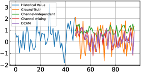
(a) Experimental results

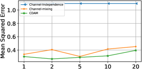
(b) Performance under different $\sigma$ during training

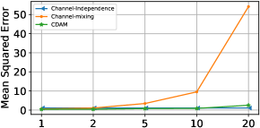
(c) Performance under different $\sigma$ during testing

Figure 5: Experimental results on synthetic data.

The experimental results on synthetic data are presented in Figure 5. Since the Channel-Independence model only takes into account the historical value and variables such as $A,\omega,\varphi,x$ change over time and are not fixed, its performance is notably inferior to that of the Channel-mixing model and CDAM. Additionally, we conducted experiments to investigate the impact of noise by training these three models using different noise levels, manipulated through the adjustment of $\sigma$, while maintaining a consistent $\sigma$ during testing. The experimental results are shown in Figure 5 (b). We observed that when the noise in the training set and the test set follows the same distribution, noise has a minimal effect on the models’ performance, resulting in only a slight reduction. Notably, compared to the Channel-mixing model, our CDAM model performs consistently well across various noise levels. To further demonstrate the noise reduction capability of CDAM, we set $\sigma=1$ during training and modified the variance $\sigma$ during testing. As depicted in Figure 5 (c), we observed that the performance of CDAM remains relatively stable, while the effectiveness of the Channel-mixing model is significantly impacted. This observation highlights the ability of CDAM to effectively minimize the influence of irrelevant noise, despite the fact that complete elimination is not achieved.

A.4 Lower bound for $I(X^{i},Y^{i};Z^{i})$

A.4.1 Derivation of $I(X^{i},Y^{i};Z^{i})$

The joint Mutual Information between the i-th historical series $X^{i}$, i-th future series $Y^{i}$ and latent representation $Z^{i}$ is defined as:

$$I(X^{i},Y^{i};Z^{i}) =I(X^{i};Z^{i})+I(Z^{i};Y^{i}|X^{i})$$ (12)

$$=\int p(z^{i},x^{i})\log\frac{p(z^{i},x^{i})}{p(z^{i})p(x^{i})}dz^{i}dx^{i}+\int p(z^{i},y^{i},x^{i})\log\frac{p(x^{i})p(z^{i},y^{i},x^{i})}{p(z^{i},x^{i})p(y^{i},x^{i})}dz^{i}dy^{i}dx^{i}$$

$$=\int p(z^{i},y^{i},x^{i})\log\frac{p(z^{i},x^{i})}{p(z^{i})p(x^{i})}dz^{i}dy^{i}dx^{i}+\int p(z^{i},y^{i},x^{i})\log\frac{p(x^{i})p(z^{i},y^{i},x^{i})}{p(z^{i},x^{i})p(y^{i},x^{i})}dz^{i}dy^{i}dx^{i}$$

$$=\int p(z^{i},y^{i},x^{i})\log\frac{p(z^{i},y^{i},x^{i})}{p(z^{i})p(y^{i},x^{i})}dz^{i}dy^{i}dx^{i}$$

$$=\int p(z^{i},y^{i},x^{i})\log\frac{p(x^{i},y^{i}|z^{i})}{p(y^{i},x^{i})}dz^{i}dy^{i}dx^{i}$$

$$=\int p(z^{i},y^{i},x^{i})\log p(y^{i},x^{i}|z^{i})dz^{i}dy^{i}dx^{i}-\int p(z^{i},y^{i},x^{i})\log p(y^{i},x^{i})dz^{i}dy^{i}dx^{i}$$

$$=\int p(z^{i},y^{i},x^{i})\log p(y^{i}|x^{i},z^{i})p(x^{i}|z^{i})dz^{i}dy^{i}dx^{i}-\int p(y^{i},x^{i})\log p(y^{i},x^{i})dy^{i}dx^{i}$$

$$=\mathbb{E}_{p(z^{i},y^{i},x^{i})}\left[\log p(y^{i}|x^{i},z^{i})\right]+\mathbb{E}_{p(z^{i},x^{i})}\left[\log p(x^{i}|z^{i})\right]+H(Y^{i},X^{i})$$

Therefore, $I(X^{i};Y^{i};Z^{i})$ can be represented as:

$$I(X^{i},Y^{i}|Z^{i})=\mathbb{E}_{p(z^{i},y^{i},x^{i})}\left[\log p(y^{i}|x^{i},z^{i})\right]+\mathbb{E}_{p(z^{i},x^{i})}\left[\log p(x^{i}|z^{i})\right]+H(Y^{i},X^{i})\\$$ (13)

A.4.2 Variational Approximation of $I(X^{i},Y^{i};Z^{i})$

$$I(X^{i},Y^{i};Z^{i}) =\mathbb{E}_{p(z^{i},y^{i},x^{i})}\left[\log p(y^{i}|x^{i},z^{i})\right]+\mathbb{E}_{p(z^{i},x^{i})}\left[\log p(x^{i}|z^{i})\right]+\text{constant}$$ (14)

We introduce $p_{\theta}(x^{i}|z^{i})$ to be the variational approximation of $p(x^{i},y^{i})$. Since the Kullback Leibler (KL) divergence is always non-negetive, we have:

$$D_{KL}\left[p(X^{i}|Z^{i})||p_{\theta}(X^{i}|Z^{i})\right] =\int p(x^{i}|z^{i})log\frac{p(x^{i}|z^{i})}{p_{\theta}(x^{i}|z^{i})}dx^{i}\geq 0$$ (15)

$$\mathbb{E}_{p(z^{i},x^{i})}\left[\log p(x^{i}|z^{i})\right] \geq\mathbb{E}_{p(z^{i},x^{i})}\left[\log p_{\theta}(x^{i}|z^{i})\right]$$

In the same way, we have:

$$\mathbb{E}_{p(z^{i},y^{i},x^{i})}\left[\log p(y^{i}|x^{i},z^{i})\right]\geq\mathbb{E}_{p(z^{i},y^{i},x^{i})}\left[\log p_{\theta}(y^{i}|x^{i},z^{i})\right]$$ (16)

Therefore, the variational lower bound is as follows:

$$I(X^{i},Y^{i};Z^{i})-\text{constant}\geq I_{v}(X^{i},Y^{i};Z^{i})=\mathbb{E}_{p(z^{i},y^{i},x^{i})}\left[\log p_{\theta}(y^{i}|x^{i},z^{i})\right]+\mathbb{E}_{p(z^{i},x^{i})}\left[\log p_{\theta}(x^{i}|z^{i})\right]$$ (17)

$I(X^{i},Y^{i};Z^{i})$ can thus be maximized by maximizing its variational lower bound.

A.5 Derivation and variational approximation of $I(\hat{Y}_{j}^{i};Y_{j-1}^{i}|X^{i})$

The Mutual Information between the $j$-th downsampling predicted subsequence $\hat{Y}_{j}^{i}$ and $(j-1)$-th target downsampling subsequence $Y_{j-1}^{i}$ given historical sequence $X^{i}$ is defined as:

$$I(\hat{Y}_{j}^{i};Y_{j-1}^{i}|X^{i}) =\int p(\hat{y}^{i}_{j},y^{i}_{j-1},x^{i})\log\frac{p(\hat{y}_{j}^{i},y_{j-1}^{i}|x^{i})}{p(\hat{y}^{i}_{j}|x^{i})p(y^{i}_{j-1}|x^{i})}d\hat{y}^{i}_{j}dy_{j-1}^{i}dx^{i}$$ (18)

$$I(Y_{j-1}^{i};\hat{Y}_{j}^{i}|X^{i}) =\int p(y_{j-1}^{i},x^{i},\hat{y}_{j}^{i})\log\frac{p(x^{i})p(y^{i}_{j-1},\hat{y}_{j}^{i},x^{i})}{p(y_{j-1}^{i},x^{i})p(\hat{y}_{j}^{i},x^{i})}d\hat{y}_{j-1}^{i}dy_{j}^{i}dx^{i}$$ (19)

$$=\int p(y_{j-1}^{i},x^{i},\hat{y}_{j}^{i})\log\frac{p(y_{j-1}^{i}|\hat{y}_{j}^{i},x^{i})}{p(y_{j-1}^{i}|x^{i})}d\hat{y}_{j-1}^{i}dy_{j}^{i}dx^{i}$$

$$=\int p(y_{j-1}^{i},x^{i},\hat{y}_{j}^{i})\log p(y^{i}_{j-1}|\hat{y}^{i}_{j},x^{i})dy_{j-1}^{i}d\hat{y}_{j}^{i}dx^{i}+H(Y_{j-1}^{i},X^{i})$$

$$\geq\int p(y_{j-1}^{i},x^{i},\hat{y}_{j}^{i})\log p(y^{i}_{j-1}|\hat{y}^{i}_{j},x^{i})dy_{j-1}^{i}d\hat{y}_{j}^{i}dx^{i}$$

Since $p(y_{j-1}^{i}|\hat{y}_{j}^{i},x^{i})$ is intractable, we use $p_{\theta}(y_{j-1}^{i}|\hat{y}_{j}^{i},x^{i})$ to approximate $p(\hat{y}_{j}^{i}|y_{j-1}^{i},x^{i})$, therefore, we have:

$$I(Y_{j-1}^{i};\hat{Y}_{j}^{i}|X^{i}) \geq\int p(y_{j-1}^{i},x^{i},\hat{y}_{j}^{i})\log p(y^{i}_{j-1}|\hat{y}^{i}_{j},x^{i})dy_{j-1}^{i}d\hat{y}_{j}^{i}dx^{i}$$ (20)

$$\geq\int p(y^{i}_{j-1},\hat{y}^{i}_{j},x^{i})\log\frac{p(y^{i}_{j-1}|\hat{y}^{i}_{j},x^{i})p_{\theta}(y^{i}_{j-1}|\hat{y}^{i}_{j},x^{i})}{p_{\theta}(y^{i}_{j-1}|\hat{y}^{i}_{j},x^{i})}dy_{j-1}^{i}d\hat{y}_{j}^{i}dx^{i}$$

$$\geq\int p(y_{j-1}^{i},\hat{y}_{j}^{i},x^{i})\log p_{\theta}(y_{j-1}^{i}|\hat{y}_{j}^{i},x^{i})dy_{j-1}^{i}d\hat{y}_{j}^{i}dx^{i}$$

$$\geq\mathbb{E}_{p(y_{j-1}^{i},\hat{y}_{j}^{i},x^{i})}\left[p_{\theta}(y_{j-1}^{i}|\hat{y}_{j}^{i},x^{i})\right]$$

Therefore, the Mutual information $I(Y_{j-1}^{i};\hat{Y}_{j}^{i}|X^{i})$ can be maximized by maximizing $\mathbb{E}_{p(y_{j-1}^{i},\hat{y}_{j}^{i},x^{i})}\left[p_{\theta}(y_{j-1}^{i}|\hat{y}_{j}^{i},x^{i})\right]$.

A.6 Extra Experimental Results

A.6.1 Full Results of Channel-Independence models

In this section, we provide the full experimental results of Channel-Independence models in Table 6 which is an extended version of Table 2

Table 6: Multivariate long-term series forecasting results on Channel-Independence models with different prediction lengths $O\in\{96,192,336,720\}$. We set the input length $I$ as 336 for all the models. The best result is indicated in bold font. ( Avg is averaged from all four prediction lengths and Pro means the relative MSE and MAE reduction.)

Models		PatchTST				RMLP
		Original		w/Ours		Original		w/Ours
Metric		MSE	MAE	MSE	MAE	MSE	MAE	MSE	MAE
ETTh1	96	0.375	0.399	0.365	0.389	0.380	0.401	0.367	0.391
	192	0.414	0.421	0.403	0.413	0.414	0.421	0.404	0.413
	336	0.440	0.440	0.427	0.428	0.439	0.436	0.426	0.429
	720	0.460	0.473	0.433	0.453	0.470	0.471	0.439	0.459
	Avg	0.422	0.433	0.407	0.420	0.426	0.432	0.409	0.423
	Pro	-	-	3.5%	3.0%	-	-	3.9%	2.1%
ETTh2	96	0.274	0.335	0.271	0.332	0.290	0.348	0.271	0.333
	192	0.342	0.382	0.334	0.373	0.350	0.388	0.335	0.374
	336	0.365	0.404	0.357	0.395	0.374	0.410	0.358	0.395
	720	0.391	0.428	0.385	0.421	0.410	0.439	0.398	0.432
	Avg	0.343	0.387	0.337	0.380	0.356	0.396	0.34	0.384
	Pro	-	-	1.7%	1.8%	-	-	4.5%	3.0%
ETTm1	96	0.290	0.342	0.283	0.335	0.290	0.343	0.285	0.335
	192	0.332	0.369	0.322	0.359	0.329	0.368	0.322	0.359
	336	0.366	0.392	0.356	0.382	0.364	0.390	0.358	0.381
	720	0.420	0.424	0.407	0.417	0.430	0.426	0.414	0.413
	Avg	0.352	0.381	0.342	0.373	0.353	0.381	0.344	0.372
	Pro	-	-	2.8%	2.1%	-	-	2.5%	2.3%
ETTm2	96	0.165	0.255	0.161	0.250	0.177	0.263	0.162	0.252
	192	0.220	0.292	0.217	0.289	0.233	0.302	0.217	0.289
	336	0.278	0.329	0.271	0.324	0.283	0.335	0.270	0.324
	720	0.367	0.385	0.362	0.381	0.367	0.388	0.357	0.380
	Avg	0.257	0.315	0.252	0.311	0.265	0.322	0.251	0.311
	Pro	-	-	1.9%	1.3%	-	-	5.2%	3.4%
Weather	96	0.152	0.199	0.144	0.194	0.147	0.198	0.144	0.196
	192	0.197	0.243	0.189	0.238	0.190	0.239	0.187	0.237
	336	0.250	0.284	0.239	0.279	0.243	0.280	0.239	0.277
	720	0.320	0.335	0.312	0.331	0.320	0.332	0.316	0.330
	Avg	0.229	0.265	0.221	0.260	0.225	0.262	0.221	0.260
	Pro	-	-	3.5%	1.8%	-	-	1.6%	0.9%
Traffic	96	0.367	0.251	0.358	0.245	0.383	0.269	0.364	0.249
	192	0.385	0.259	0.379	0.254	0.401	0.276	0.384	0.258
	336	0.398	0.265	0.391	0.261	0.414	0.282	0.398	0.266
	720	0.434	0.287	0.425	0.280	0.443	0.309	0.428	0.284
	Avg	0.396	0.265	0.388	0.260	0.410	0.284	0.393	0.264
	Pro	-	-	2.0%	1.8%	-	-	5.2%	8.4%
Electricity	96	0.130	0.222	0.125	0.219	0.130	0.225	0.125	0.218
	192	0.148	0.242	0.143	0.235	0.148	0.240	0.144	0.236
	336	0.167	0.261	0.161	0.255	0.164	0.257	0.160	0.253
	720	0.202	0.291	0.198	0.287	0.203	0.291	0.195	0.285
	Avg	0.161	0.254	0.156	0.249	0.161	0.253	0.156	0.248
	Pro	-	-	3.1%	1.9%	-	-	3.1%	2.1%

A.6.2 Additional Ablation Study

In this section, we provide the full ablation experimental results of the Channel-mixing models and Channel-Independence models in Table LABEL:tab:ablation_dependent and Table LABEL:tab:ablation_independent, respectively, which are the extended of Table LABEL:tab:ablation. We also provide Table 9, which contains the full results of ablation experiments on the PEMS (PEMS03, PEMS04, PEMS08) dataset.

Table 7: Component ablation of InfoTime for RMLP and PatchTST. We set the input length $I$ as 336. The best results are in bold and the second best are underlined.

Models		RMLP						PatchTST
		Original		+TAM		+InfoTime		Original		+TAM		+InfoTime
Metric		MSE	MAE	MSE	MAE	MSE	MAE	MSE	MAE	MSE	MAE	MSE	MAE
ETTh1	96	0.380	0.401	0.371	0.392	0.367	0.391	0.375	0.399	0.367	0.391	0.365	0.389
	192	0.414	0.421	0.406	0.414	0.404	0.413	0.414	0.421	0.405	0.414	0.403	0.413
	336	0.439	0.436	0.427	0.428	0.426	0.429	0.440	0.440	0.429	0.430	0.427	0.428
	720	0.470	0.471	0.450	0.465	0.439	0.459	0.460	0.473	0.435	0.455	0.433	0.453
ETTh2	96	0.290	0.348	0.278	0.337	0.271	0.333	0.274	0.335	0.271	0.332	0.271	0.332
	192	0.350	0.388	0.340	0.377	0.335	0.374	0.342	0.382	0.334	0.373	0.334	0.373
	336	0.374	0.410	0.366	0.402	0.358	0.395	0.365	0.404	0.357	0.393	0.357	0.395
	720	0.410	0.439	0.404	0.435	0.398	0.432	0.391	0.428	0.386	0.422	0.385	0.421
ETTm1	96	0.290	0.343	0.285	0.337	0.285	0.335	0.290	0.342	0.286	0.337	0.283	0.335
	192	0.329	0.368	0.321	0.360	0.322	0.359	0.332	0.369	0.326	0.366	0.322	0.359
	336	0.364	0.390	0.357	0.382	0.358	0.381	0.366	0.392	0.359	0.388	0.356	0.382
	720	0.430	0.426	0.415	0.415	0.414	0.413	0.420	0.424	0.408	0.413	0.407	0.417
ETTm2	96	0.177	0.263	0.166	0.255	0.162	0.252	0.165	0.255	0.162	0.251	0.161	0.250
	192	0.233	0.302	0.222	0.294	0.217	0.289	0.220	0.292	0.218	0.290	0.217	0.289
	336	0.283	0.335	0.274	0.328	0.270	0.324	0.278	0.329	0.273	0.326	0.271	0.324
	720	0.367	0.388	0.362	0.384	0.357	0.380	0.367	0.385	0.364	0.382	0.362	0.381
Weather	96	0.147	0.198	0.146	0.197	0.144	0.196	0.152	0.199	0.149	0.197	0.144	0.194
	192	0.190	0.239	0.189	0.238	0.187	0.237	0.197	0.243	0.192	0.238	0.189	0.238
	336	0.243	0.280	0.241	0.278	0.239	0.277	0.250	0.284	0.247	0.280	0.239	0.279
	720	0.320	0.332	0.319	0.332	0.316	0.330	0.320	0.335	0.321	0.332	0.312	0.331
Traffic	96	0.383	0.269	0.366	0.252	0.364	0.249	0.367	0.251	0.359	0.245	0.358	0.245
	192	0.401	0.276	0.386	0.260	0.384	0.258	0.385	0.259	0.380	0.255	0.379	0.254
	336	0.414	0.282	0.400	0.268	0.398	0.266	0.398	0.265	0.391	0.262	0.391	0.261
	720	0.443	0.309	0.432	0.286	0.428	0.284	0.434	0.287	0.424	0.279	0.425	0.280
Electricity	96	0.130	0.225	0.127	0.221	0.125	0.218	0.130	0.222	0.129	0.223	0.125	0.219
	192	0.148	0.240	0.145	0.238	0.144	0.236	0.148	0.242	0.147	0.240	0.143	0.235
	336	0.164	0.257	0.162	0.255	0.160	0.253	0.167	0.261	0.165	0.258	0.161	0.255
	720	0.203	0.291	0.199	0.288	0.195	0.285	0.202	0.291	0.204	0.292	0.198	0.287

Table 8: Component ablation of InfoTime for Informer, Stationary, and Crossformer. We set the input length $I$ as 96. The best results are in bold and the second best are underlined.

Models		Informer						Stationary						Crossformer
		Original		+TAM		+InfoTime		Original		+TAM		+InfoTime		Original		+TAM		+InfoTime
Metric		MSE	MAE	MSE	MAE	MSE	MAE	MSE	MAE	MSE	MAE	MSE	MAE	MSE	MAE	MSE	MAE	MSE	MAE
ETTh1	96	0.865	0.713	0.598	0.565	0.381	0.394	0.598	0.498	0.455	0.452	0.375	0.388	0.457	0.463	0.396	0.411	0.379	0.392
	192	1.008	0.792	0.694	0.640	0.435	0.430	0.602	0.520	0.491	0.478	0.425	0.417	0.635	0.581	0.541	0.511	0.433	0.427
	336	1.107	0.809	0.853	0.719	0.485	0.461	0.677	0.573	0.611	0.530	0.463	0.436	0.776	0.667	0.759	0.651	0.482	0.458
	720	1.181	0.865	0.914	0.741	0.534	0.524	0.719	0.597	0.594	0.542	0.463	0.459	0.861	0.725	0.845	0.711	0.529	0.517
ETTh2	96	3.755	1.525	0.502	0.538	0.336	0.390	0.362	0.393	0.330	0.371	0.286	0.335	0.728	0.615	0.364	0.415	0.333	0.386
	192	5.602	1.931	0.821	0.701	0.468	0.470	0.481	0.453	0.456	0.440	0.371	0.388	0.898	0.705	0.470	0.481	0.455	0.453
	336	4.721	1.835	1.065	0.823	0.582	0.534	0.524	0.487	0.475	0.463	0.414	0.425	1.132	0.807	0.580	0.547	0.554	0.513
	720	3.647	1.625	1.489	1.022	0.749	0.620	0.512	0.494	0.506	0.486	0.418	0.437	4.390	1.795	0.768	0.648	0.757	0.619
ETTm1	96	0.672	0.571	0.435	0.444	0.326	0.367	0.396	0.401	0.375	0.396	0.326	0.362	0.385	0.409	0.388	0.401	0.323	0.362
	192	0.795	0.669	0.473	0.467	0.371	0.391	0.471	0.436	0.441	0.432	0.366	0.379	0.459	0.478	0.436	0.428	0.366	0.386
	336	1.212	0.871	0.545	0.518	0.408	0.416	0.517	0.464	0.472	0.455	0.392	0.398	0.645	0.583	0.483	0.457	0.403	0.414
	720	1.166	0.823	0.669	0.589	0.482	0.464	0.664	0.527	0.532	0.489	0.455	0.434	0.756	0.669	0.548	0.498	0.473	0.460
ETTm2	96	0.365	0.453	0.258	0.378	0.187	0.282	0.201	0.291	0.185	0.276	0.175	0.256	0.281	0.373	0.223	0.321	0.186	0.281
	192	0.533	0.563	0.439	0.515	0.277	0.351	0.275	0.335	0.254	0.318	0.238	0.297	0.549	0.520	0.347	0.404	0.269	0.341
	336	1.363	0.887	0.836	0.728	0.380	0.420	0.350	0.377	0.343	0.372	0.299	0.336	0.729	0.603	0.528	0.506	0.356	0.396
	720	3.379	1.338	3.172	1.322	0.607	0.549	0.460	0.435	0.440	0.421	0.398	0.393	1.059	0.741	0.895	0.665	0.493	0.482
Weather	96	0.300	0.384	0.277	0.354	0.179	0.249	0.181	0.230	0.178	0.226	0.166	0.213	0.158	0.236	0.154	0.225	0.149	0.218
	192	0.598	0.544	0.407	0.447	0.226	0.296	0.286	0.312	0.261	0.296	0.218	0.260	0.209	0.285	0.202	0.27	0.202	0.272
	336	0.578	0.523	0.529	0.520	0.276	0.334	0.319	0.335	0.318	0.333	0.274	0.300	0.265	0.328	0.263	0.320	0.256	0.313
	720	1.059	0.741	0.951	0.734	0.332	0.372	0.411	0.393	0.387	0.378	0.351	0.353	0.376	0.397	0.353	0.382	0.329	0.366
Traffic	96	0.719	0.391	0.577	0.356	0.505	0.348	0.599	0.332	0.503	0.313	0.459	0.311	0.609	0.362	0.490	0.308	0.529	0.334
	192	0.696	0.379	0.556	0.357	0.521	0.354	0.619	0.341	0.488	0.309	0.475	0.315	0.623	0.365	0.493	0.310	0.519	0.327
	336	0.777	0.420	0.580	0.370	0.520	0.337	0.651	0.347	0.506	0.318	0.486	0.319	0.649	0.370	0.53	0.328	0.521	0.337
	720	0.864	0.472	0.668	0.430	0.552	0.352	0.658	0.358	0.542	0.329	0.522	0.338	0.758	0.418	0.591	0.348	0.556	0.350
Electricity	96	0.274	0.368	0.228	0.333	0.195	0.300	0.168	0.271	0.152	0.252	0.154	0.256	0.170	0.279	0.151	0.251	0.150	0.248
	192	0.296	0.386	0.238	0.344	0.193	0.291	0.186	0.285	0.166	0.265	0.163	0.263	0.198	0.303	0.168	0.266	0.168	0.263
	336	0.300	0.394	0.254	0.358	0.206	0.300	0.194	0.297	0.180	0.280	0.178	0.279	0.235	0.328	0.197	0.292	0.200	0.290
	720	0.373	0.439	0.288	0.379	0.241	0.332	0.224	0.316	0.208	0.305	0.201	0.299	0.27	0.36	0.238	0.328	0.235	0.323

Table 9: Component ablation of InfoTime for PatchTST, RMLP, Informer, Stationary, and Crossformer on PEMS (PEMS03, PEMS04, and PEMS08) datasets. We set the input length $I$ as 336 for all of these base models.

Models		Metric	PEMS03				PEMS04				PEMS08
			96	192	336	720	96	192	336	720	96	192	336	720
PatchTST	Original	MSE	0.180	0.207	0.223	0.291	0.195	0.218	0.237	0.321	0.239	0.292	0.314	0.372
		MAE	0.281	0.295	0.309	0.364	0.296	0.314	0.329	0.394	0.324	0.351	0.374	0.425
	+TAM	MSE	0.159	0.189	0.193	0.263	0.170	0.198	0.204	0.257	0.186	0.244	0.257	0.307
		MAE	0.270	0.293	0.286	0.350	0.276	0.297	0.299	0.345	0.289	0.324	0.320	0.378
	+InfoTime	MSE	0.115	0.154	0.164	0.198	0.110	0.118	0.129	0.149	0.114	0.160	0.177	0.209
		MAE	0.223	0.251	0.256	0.286	0.221	0.224	0.237	0.261	0.218	0.243	0.241	0.281
RMLP	Original	MSE	0.160	0.184	0.201	0.254	0.175	0.199	0.210	0.255	0.194	0.251	0.274	0.306
		MAE	0.257	0.277	0.291	0.337	0.278	0.294	0.306	0.348	0.279	0.311	0.328	0.365
	+TAM	MSE	0.143	0.171	0.186	0.234	0.153	0.181	0.189	0.222	0.158	0.215	0.236	0.264
		MAE	0.241	0.264	0.276	0.316	0.259	0.280	0.289	0.321	0.255	0.288	0.302	0.333
	+InfoTime	MSE	0.117	0.159	0.146	0.204	0.103	0.114	0.130	0.154	0.116	0.156	0.175	0.181
		MAE	0.228	0.252	0.246	0.285	0.211	0.219	0.236	0.264	0.215	0.235	0.242	0.255
Informer	Original	MSE	0.139	0.152	0.165	0.216	0.132	0.146	0.147	0.145	0.156	0.175	0.187	0.264
		MAE	0.240	0.252	0.260	0.290	0.238	0.249	0.247	0.245	0.262	0.266	0.274	0.325
	+TAM	MSE	0.126	0.142	0.157	0.207	0.118	0.128	0.134	0.138	0.126	0.149	0.172	0.237
		MAE	0.230	0.245	0.254	0.284	0.226	0.232	0.235	0.240	0.232	0.247	0.265	0.316
	+InfoTime	MSE	0.109	0.120	0.144	0.194	0.107	0.124	0.124	0.136	0.099	0.123	0.147	0.196
		MAE	0.216	0.228	0.247	0.282	0.215	0.230	0.231	0.245	0.204	0.224	0.242	0.278
Stationary	Original	MSE	0.120	0.143	0.156	0.220	0.109	0.116	0.129	0.139	0.151	0.180	0.252	0.223
		MAE	0.222	0.242	0.252	0.300	0.214	0.220	0.230	0.240	0.235	0.247	0.262	0.285
	+TAM	MSE	0.118	0.143	0.156	0.208	0.104	0.115	0.123	0.136	0.134	0.160	0.191	0.231
		MAE	0.219	0.241	0.252	0.285	0.209	0.218	0.223	0.234	0.224	0.237	0.251	0.289
	+InfoTime	MSE	0.101	0.131	0.153	0.190	0.096	0.114	0.125	0.135	0.103	0.144	0.184	0.217
		MAE	0.206	0.229	0.245	0.273	0.199	0.217	0.229	0.243	0.200	0.220	0.245	0.278
Crossformer	Original	MSE	0.159	0.233	0.275	0.315	0.149	0.216	0.230	0.276	0.141	0.162	0.199	0.261
		MAE	0.270	0.319	0.351	0.383	0.261	0.320	0.324	0.369	0.253	0.269	0.306	0.355
	+TAM	MSE	0.134	0.179	0.217	0.264	0.133	0.171	0.186	0.240	0.112	0.136	0.156	0.196
		MAE	0.237	0.270	0.298	0.335	0.237	0.270	0.284	0.329	0.220	0.235	0.252	0.289
	+InfoTime	MSE	0.119	0.166	0.189	0.223	0.114	0.139	0.161	0.171	0.088	0.108	0.134	0.171
		MAE	0.217	0.250	0.265	0.293	0.215	0.236	0.258	0.275	0.190	0.206	0.222	0.251

References

- Alemi et al. (2016) Alemi, A. A., Fischer, I., Dillon, J. V., and Murphy, K. Deep variational information bottleneck. arXiv preprint arXiv:1612.00410, 2016.
- Bahadori & Lipton (2019) Bahadori, M. T. and Lipton, Z. C. Temporal-clustering invariance in irregular healthcare time series. arXiv preprint arXiv:1904.12206, 2019.
- Bai et al. (2020) Bai, L., Yao, L., Li, C., Wang, X., and Wang, C. Adaptive graph convolutional recurrent network for traffic forecasting. Advances in neural information processing systems, 33:17804–17815, 2020.
- Belghazi et al. (2018) Belghazi, M. I., Baratin, A., Rajeshwar, S., Ozair, S., Bengio, Y., Courville, A., and Hjelm, D. Mutual information neural estimation. In International conference on machine learning, pp. 531–540. PMLR, 2018.
- Box et al. (2015) Box, G. E., Jenkins, G. M., Reinsel, G. C., and Ljung, G. M. Time series analysis: forecasting and control. John Wiley & Sons, 2015.
- Butte & Kohane (1999) Butte, A. J. and Kohane, I. S. Mutual information relevance networks: functional genomic clustering using pairwise entropy measurements. In Biocomputing 2000, pp. 418–429. World Scientific, 1999.
- Chen et al. (2001) Chen, C., Petty, K., Skabardonis, A., Varaiya, P., and Jia, Z. Freeway performance measurement system: mining loop detector data. Transportation Research Record, 1748(1):96–102, 2001.
- Chen et al. (2021) Chen, M., Peng, H., Fu, J., and Ling, H. Autoformer: Searching transformers for visual recognition. In Proceedings of the IEEE/CVF international conference on computer vision, pp. 12270–12280, 2021.
- Cheng et al. (2020) Cheng, P., Hao, W., Dai, S., Liu, J., Gan, Z., and Carin, L. Club: A contrastive log-ratio upper bound of mutual information. In International conference on machine learning, pp. 1779–1788. PMLR, 2020.
- Federici et al. (2020) Federici, M., Dutta, A., Forré, P., Kushman, N., and Akata, Z. Learning robust representations via multi-view information bottleneck. arXiv preprint arXiv:2002.07017, 2020.
- Franceschi et al. (2019) Franceschi, J.-Y., Dieuleveut, A., and Jaggi, M. Unsupervised scalable representation learning for multivariate time series. Advances in neural information processing systems, 32, 2019.
- Goyal et al. (2019) Goyal, A., Islam, R., Strouse, D., Ahmed, Z., Botvinick, M., Larochelle, H., Bengio, Y., and Levine, S. Infobot: Transfer and exploration via the information bottleneck. arXiv preprint arXiv:1901.10902, 2019.
- Hjelm et al. (2018) Hjelm, R. D., Fedorov, A., Lavoie-Marchildon, S., Grewal, K., Bachman, P., Trischler, A., and Bengio, Y. Learning deep representations by mutual information estimation and maximization. arXiv preprint arXiv:1808.06670, 2018.
- Igl et al. (2019) Igl, M., Ciosek, K., Li, Y., Tschiatschek, S., Zhang, C., Devlin, S., and Hofmann, K. Generalization in reinforcement learning with selective noise injection and information bottleneck. Advances in neural information processing systems, 32, 2019.
- Kim et al. (2021) Kim, T., Kim, J., Tae, Y., Park, C., Choi, J.-H., and Choo, J. Reversible instance normalization for accurate time-series forecasting against distribution shift. In International Conference on Learning Representations, 2021.
- Kwak & Choi (2002) Kwak, N. and Choi, C.-H. Input feature selection by mutual information based on parzen window. IEEE transactions on pattern analysis and machine intelligence, 24(12):1667–1671, 2002.
- Lai et al. (2018) Lai, G., Chang, W.-C., Yang, Y., and Liu, H. Modeling long-and short-term temporal patterns with deep neural networks. In The 41st international ACM SIGIR conference on research & development in information retrieval, pp. 95–104, 2018.
- Langley (2000) Langley, P. Crafting papers on machine learning. In Langley, P. (ed.), Proceedings of the 17th International Conference on Machine Learning (ICML 2000), pp. 1207–1216, Stanford, CA, 2000. Morgan Kaufmann.
- Lea et al. (2017) Lea, C., Flynn, M. D., Vidal, R., Reiter, A., and Hager, G. D. Temporal convolutional networks for action segmentation and detection. In proceedings of the IEEE Conference on Computer Vision and Pattern Recognition, pp. 156–165, 2017.
- Li et al. (2019) Li, S., Jin, X., Xuan, Y., Zhou, X., Chen, W., Wang, Y.-X., and Yan, X. Enhancing the locality and breaking the memory bottleneck of transformer on time series forecasting. Advances in neural information processing systems, 32, 2019.
- Lin et al. (2023) Lin, S., Lin, W., Wu, W., Wang, S., and Wang, Y. Petformer: Long-term time series forecasting via placeholder-enhanced transformer. arXiv preprint arXiv:2308.04791, 2023.
- Liu et al. (2018) Liu, H., He, L., Bai, H., Dai, B., Bai, K., and Xu, Z. Structured inference for recurrent hidden semi-markov model. In Lang, J. (ed.), Proceedings of the Twenty-Seventh International Joint Conference on Artificial Intelligence, IJCAI 2018, July 13-19, 2018, Stockholm, Sweden, pp. 2447–2453, 2018.
- Liu et al. (2022a) Liu, M., Zeng, A., Chen, M., Xu, Z., Lai, Q., Ma, L., and Xu, Q. Scinet: Time series modeling and forecasting with sample convolution and interaction. Advances in Neural Information Processing Systems, 35:5816–5828, 2022a.
- Liu et al. (2022b) Liu, Y., Wu, H., Wang, J., and Long, M. Non-stationary transformers: Exploring the stationarity in time series forecasting. Advances in Neural Information Processing Systems, 35:9881–9893, 2022b.
- Luo et al. (2019) Luo, Y., Liu, P., Guan, T., Yu, J., and Yang, Y. Significance-aware information bottleneck for domain adaptive semantic segmentation. In Proceedings of the IEEE/CVF International Conference on Computer Vision, pp. 6778–6787, 2019.
- Mahabadi et al. (2021) Mahabadi, R. K., Belinkov, Y., and Henderson, J. Variational information bottleneck for effective low-resource fine-tuning. arXiv preprint arXiv:2106.05469, 2021.
- Murphy & Chen (2022) Murphy, W. M. J. and Chen, K. Univariate vs multivariate time series forecasting with transformers. 2022.
- Nie et al. (2022) Nie, Y., Nguyen, N. H., Sinthong, P., and Kalagnanam, J. A time series is worth 64 words: Long-term forecasting with transformers. arXiv preprint arXiv:2211.14730, 2022.
- Oord et al. (2018) Oord, A. v. d., Li, Y., and Vinyals, O. Representation learning with contrastive predictive coding. arXiv preprint arXiv:1807.03748, 2018.
- Poole et al. (2019) Poole, B., Ozair, S., Van Den Oord, A., Alemi, A., and Tucker, G. On variational bounds of mutual information. In International Conference on Machine Learning, pp. 5171–5180. PMLR, 2019.
- Rangapuram et al. (2018) Rangapuram, S. S., Seeger, M. W., Gasthaus, J., Stella, L., Wang, Y., and Januschowski, T. Deep state space models for time series forecasting. Advances in neural information processing systems, 31, 2018.
- Salinas et al. (2020) Salinas, D., Flunkert, V., Gasthaus, J., and Januschowski, T. Deepar: Probabilistic forecasting with autoregressive recurrent networks. International Journal of Forecasting, 36(3):1181–1191, 2020.
- Schulz et al. (2020) Schulz, K., Sixt, L., Tombari, F., and Landgraf, T. Restricting the flow: Information bottlenecks for attribution. arXiv preprint arXiv:2001.00396, 2020.
- Shwartz-Ziv & Tishby (2017) Shwartz-Ziv, R. and Tishby, N. Opening the black box of deep neural networks via information. arXiv preprint arXiv:1703.00810, 2017.
- Tishby & Zaslavsky (2015) Tishby, N. and Zaslavsky, N. Deep learning and the information bottleneck principle. In 2015 ieee information theory workshop (itw), pp. 1–5. IEEE, 2015.
- Tishby et al. (2000) Tishby, N., Pereira, F. C., and Bialek, W. The information bottleneck method. arXiv preprint physics/0004057, 2000.
- Voita et al. (2019) Voita, E., Sennrich, R., and Titov, I. The bottom-up evolution of representations in the transformer: A study with machine translation and language modeling objectives. arXiv preprint arXiv:1909.01380, 2019.
- West et al. (2019) West, P., Holtzman, A., Buys, J., and Choi, Y. Bottlesum: Unsupervised and self-supervised sentence summarization using the information bottleneck principle. arXiv preprint arXiv:1909.07405, 2019.
- Zeng et al. (2022) Zeng, A., Chen, M., Zhang, L., and Xu, Q. Are transformers effective for time series forecasting? arXiv preprint arXiv:2205.13504, 2022.
- (40) Zhang, Y. and Yan, J. Crossformer: Transformer utilizing cross-dimension dependency for multivariate time series forecasting. In The Eleventh International Conference on Learning Representations.
- Zhou et al. (2021) Zhou, H., Zhang, S., Peng, J., Zhang, S., Li, J., Xiong, H., and Zhang, W. Informer: Beyond efficient transformer for long sequence time-series forecasting. In Proceedings of the AAAI conference on artificial intelligence, volume 35, pp. 11106–11115, 2021.
- Zhou et al. (2022) Zhou, T., Ma, Z., Wen, Q., Wang, X., Sun, L., and Jin, R. Fedformer: Frequency enhanced decomposed transformer for long-term series forecasting. In International Conference on Machine Learning, pp. 27268–27286. PMLR, 2022.