Higher vortexability: zero field realization of higher Landau levels

Abstract

The rise of moiré materials has led to experimental realizations of integer and FCIs in small or vanishing magnetic fields. At the same time, a set of minimal conditions sufficient to guarantee an Abelian fractional state in a flat band were identified, namely “ideal" or “vortexable" quantum geometry. Such vortexable bands share essential features with the LLL, while excluding the need for more fine-tuned aspects such as flat Berry curvature. A natural and important generalization is to ask if such conditions can be extended to capture the quantum geometry of higher Landau levels, particularly the first (1LL), where non-Abelian states at $\nu=1/2,2/5$ are known to be competitive. The possibility of realizing these states at zero magnetic field, and perhaps even more exotic ones, could become a reality if we could identify the essential structure of the 1LL in Chern bands. In this work, we introduce a precise definition of 1LL quantum geometry, along with a figure of merit that measures how closely a given band approaches the 1LL. Periodically strained Bernal graphene is shown to realize such a 1LL structure even in zero magnetic field.

Fractional Chern Insulators (FCIs) [1, 2, 3, 4, 5, 6, 7, 8, 9, 10] realize the fractionalized charges and anyonic statistics associated with fractional quantum Hall physics in Chern bands. Such states do not require a magnetic field and can potentially form at much higher temperatures [11, 12, 13, 14, 15, 16, 17]. They were observed in Harper-Hofstadter bands [11] at high magnetic field, and in the partially filled Chern bands of twisted bilayer graphene with the help of a small magnetic field [12]. Not only does the field reduce the bandwidth [18], but it was also argued to improve the wavefunctions of the Chern band, pushing them to an “ideal" or “vortexable" limit where the band becomes a modulated version of the lowest LL (LLL) [19, 20, 21, 22, 23, 24, 25, 26, 27, 28]. More recently, Abelian FCIs at zero magnetic field, dubbed fractional quantum anomalous Hall (FQAH) states, were observed in twisted MoTe2 [13, 14, 15, 16], following theoretical works showcasing small bandwidths and numerical works finding FCI ground states [29, 30, 31, 32, 33, 34, 35, 36, 37, 38, 39, 40, 41, 42, 43], and also in pentalayer graphene [17, 44, 45, 46, 47, 48, 49]. As these zero field devices improve, they will likely run the gamut of Abelian topological orders found in the LLL.

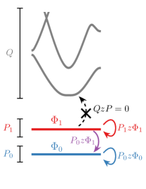
Figure 1: Cartoon depicting the definition, (4), of a first vortexable band, with band projector $P_{1}$.

To date, experimental realizations of non-Abelian topological order are the almost-exclusive province of the first LL. Namely, the half-filled first LL in GaAs [50, 51, 52] and Bernal graphene [53, 54, 55, 56, 57] realize a Pfaffian-type state with non-Abelian particle statistics[58]. Also, the plateau at $\nu=2+2/5$ in GaAs [59] may be a non-Abelian phase harboring Fibonacci anyons [60], a scenario that has received numerical support  [60, 61]. Beyond their immense theoretical importance, such states have practical utility as a platform for fault-tolerant quantum computation [62, 63]. Realizing non-Abelian states in Chern bands, at energy scales unachievable with external magnetic field, would be especially useful in this context. This raises the question — are there Chern bands at zero magnetic field analogous to the first LL?

In this work we answer this question by providing a precise definition of what it means for a band to be similar to the first LL. Our definition makes use of “vortexability" applied to multi-band systems. A Chern band has first LL structure if we can find a partner band with a zeroth LL structure such that the two bands taken together are vortexable. Vortex attachment applied to both bands produces exact Jain-like [64] ground states in the limit of short-range repulsive interactions, without the need for further projection when the bands are degenerate. In general, the partner band is not required to be nearby in energy. We argue that single-band definitions, such as those based on the Fubini-Study metric used for the LLL case [65], cannot capture first LL structure. Below we motivate and explicate our definition, then provide a concrete example in zero-field superlattice system, periodically strained Bernal graphene. Our construction is readily extendable to higher Chern bands, by forming $(n+1)$ Chern band complexes to capture the geometry of the ‘$n$th’ LL.

LLL-type Quantum Geometry Review— We begin by reviewing the point of view that has recently emerged on “LLL band geometry," through ideal, or vortexable, Chern bands [19, 23, 20, 21, 22, 66, 67, 24, 25, 28, 68, 69, 26, 27, 70]. These names refer to the following equivalent criteria. (i) The bands are vortexable [24, 28]: $z\psi=Pz\psi$, where $P$ is the projector onto the band(s) of interest, $\psi=P\psi$ is a wavefunction in those bands, and $z=x+iy$ is the vortex function. (ii) The bands satisfy the trace condition $\operatorname{tr}g({\bm{k}})=\Omega({\bm{k}})$ [71, 10], where $g_{\mu\nu}({\bm{k}})$ is the Fubini-Study metric and $\Omega({\bm{k}})$ is the Berry curvature. (iii) The cell-periodic states $u_{{\bm{k}}a}({\bm{r}})=e^{-i{\bm{k}}\cdot{\bm{r}}}\psi_{{\bm{k}}a}({\bm{r}})$ can be written as holomorphic functions of $k=k_{x}+ik_{y}$ up to orthonormality (here “$a$" is a band index) [72, 73, 22]. More general vortex functions [28] with correspondingly generalized trace conditions (suitable for other unit cell embeddings [74]) are omitted here for concision. For zero dispersion vortexable bands, Laughlin-like trial states constructed by attaching vortices (i.e. Jastrow factors) $\prod_{i<j}(z_{i}-z_{j})^{2m}$ to integer filling states are exact many-body ground states in the limit of short range repulsive interactions [75, 19, 28]. Thus, these generalizations of the LLL provide a frustration-free route to realizing the Laughlin states. Note, in contrast to naive intuition and early work on FCIs, homogeneous Berry curvature is not a requirement.

Wavefunctions for $C=1$ ideal bands have the form [19, 23]

$$\psi({\bm{r}})=f(z)\mathcal{N}_{0}({\bm{r}});\quad\mathcal{N}_{0}^{l}({\bm{r}})=e^{-K({\bm{r}})}\zeta^{l}({\bm{r}})$$ (1)

where $f(z)$ is holomorphic, $\zeta^{l}({\bm{r}})$ is an orbital-space spinor (with layer index $l$, e.g.), and $\phi({\bm{r}})=f(z)e^{-K({\bm{r}})}$ is a zero mode of a Dirac particle in the inhomogeneous magnetic field $B({\bm{r}})=\nabla^{2}\operatorname{Re}K({\bm{r}})$. Due to its normalization $\sum_{l}\lvert\zeta^{l}({\bm{r}})\rvert^{2}=1$ the spinor part does not influence the energy of the band under density-density interactions, and can thus be largely ignored for our purposes. The class of $C=1$ vortexable bands therefore has the same analytic structure as the LLL in an inhomogenous magnetic field and metric that breaks continuous translation symmetry [19, 69]. Vortexability is thus a sufficient condition for a Chern band to be “analogous to the LLL".

First Landau Levels Are Diverse— To extend the success of ideal bands to the first LL, one could imagine imposing band geometric criteria to mimic a 1LL features. For example, the first LL of a $p^{2}/2m$ particle has $\operatorname{tr}g=3\Omega$ [21]. However, this and other approaches fail to capture the wide spectrum of “first LLs" in multilayer graphene. To wit, we recall Bernal graphene at $B>0$:

$$H_{\rm BG}=\left(\begin{array}[]{cc}0&D_{1}^{\dagger}\\ D_{1}&0\end{array}\right),\quad D_{1}=\left(\begin{array}[]{cc}D_{0}&\gamma_{1}\\ 0&D_{0}\end{array}\right),$$ (2)

written in the chiral basis $(|A,1\rangle,|A,2\rangle,|B,1\rangle,|B,2\rangle)$. Here $D_{0}=2v\left(-i\bar{\partial}_{z}-\bar{A}_{z}\right)=\sqrt{2}vl_{B}^{-1}\hat{a}$ is proportional to the annihilation operator and $\gamma_{1}$ is the interlayer coupling. There are two bands of zero modes; $\ker D_{1}$ is spanned by

$$\Phi_{0}=\left(\begin{array}[]{c}\psi_{0}\\ 0\end{array}\right),\quad\Phi_{1}=\left(\begin{array}[]{c}v^{-1}\ell_{B}\gamma_{1}\hat{a}^{\dagger}\psi_{0}\\ -\sqrt{2}\psi_{0}\end{array}\right),$$ (3)

forming a zeroth and first LL respectively, where $\psi_{0}({\bm{r}})=f(z)e^{-\lvert z\rvert^{2}/4\ell_{B}^{2}}$ in symmetric gauge with $f(z)$ holomorphic.

Direct computation shows that, as $\gamma_{1}$ varies from $0$ to $\infty$, the ratio $\operatorname{tr}g_{1}/\Omega_{1}$ of band $\Phi_{1}$ varies continuously from $1$ to $3$. However, the wavefunctions have a similar analytic structure throughout. Even if one insists the first LL corresponds only to the $\gamma_{1}\to\infty$ limit, with $\operatorname{tr}g_{1}=3\Omega_{1}$, the condition $\operatorname{tr}g=3\Omega$ is also satisfied by the second LL of trilayer graphene for a particular value of $v^{-1}\ell_{B}\gamma_{1}$. The single-band Berry curvature and quantum metric therefore appear insufficient to specify a first LL structure.

The fact that the first $n$ LLs are ideal, when taken together, was first noticed in [21] by explicitly calculating $\operatorname{tr}g=\Omega$ for a $p^{2}/2m$ particle. This property that adding vortices to the first LL gives components in both first and zeroth LLs is the crux of our generalization.

Definition of First LL Structure— We now precisely define the structure bands must satisfy to be “first LL analogues". A Chern band, with projector $P_{1}$, is first vortexable if the following two conditions are satisfied:

1. ($\exists$ Partner Band) There exists an orthogonal vortexable band with projector $P_{0}$ (i.e. $P_{0}z\Phi_{0}~{}=~{}z\Phi_{0}$ for all $P_{0}\Phi_{0}=\Phi_{0}$) such that

   $$(P_{1}+P_{0})z\Phi_{1} =z\Phi_{1}$$ (4)

   for all states $P_{1}\Phi_{1}=\Phi_{1}$.

2. (Indecomposability) there is no alternative basis of wavefunctions $(\Phi_{0,{\bm{k}}}^{\prime},\Phi_{1,{\bm{k}}}^{\prime})$, where each band is vortexable, that also spans the two band subspace of $P_{0}+P_{1}$.

The additional band, described by the projector $P_{0}$, functions as an effective zeroth LL. Intuitively, acting with $z$ either keeps the wavefunction within the ‘first’ band $P_{1}$ or lowers it to the ‘zeroth’ band $P_{0}$ — but does not generate components in any other bands (see Fig. 1a). The second condition is in principle necessary to avoid subtle situations where the first condition can nominally be realized, but the system should be thought of as a collection of two separate, individually vortexable, bands instead.

While the definition above may appear computationally difficult to verify the wavefunctions that satisfy it are tightly restricted. Our constructions will all yield wavefunctions of the form

$$\Phi_{1}({\bm{r}})=Q_{0}\left[\left(\overline{z}f(z)-2B_{0}^{-1}f^{\prime}(z)\right)\mathcal{N}_{0}({\bm{r}})+f(z)\mathcal{N}_{1}({\bm{r}})\right]$$ (5)

which will be proven to be general in Ref. [76]. Here $Q_{0}=1-P_{0}$, $\mathcal{N}_{0,1}$ are spinor-valued [cf. Eq. (1)], and $P_{0}$ is the projector onto the “zeroth-LL" wavefunctions $f(z)\mathcal{N}_{0}({\bm{r}})$. $B_{0}=\frac{2\pi}{A_{\mathrm{UC}}}=\frac{A_{\mathrm{BZ}}}{2\pi}$, and $A_{\mathrm{UC}}$ and $A_{\mathrm{BZ}}$ are the areas of the unit cell and the Brillouin Zone (BZ), respectively. In Appendix E, we prove that bands with wavefunctions (5) are first vortexable. Bands that are suspected to be first vortexable can be explicitly compared to an instance (5), as we will see shortly. In Appendix A, we derive a zero-field concrete form of Eq.(5) in an analytically solvable model motivated by magic angle twisted bilayer graphene.

First vortexability has immediate many-body implications. Consider a first vortexable band that is flat and degenerate with its vortexable counterpart, as in Bernal graphene and in a upcoming example. Let $\Psi_{\nu=2}$ be the many-body state where both bands are full. Now consider the vortex attached state $\Psi_{v}=\prod_{i<j}(z_{i}-z_{j})^{2s}\Psi_{\nu=p}$ which has filling $p/(2ps+1)$, where $p=2$ (note, general $p$ follows analogously for $(p-1)$’th vortexability). Thanks to vortexability of the combined bands, attaching this vortex factor keeps the final state within the combined bands. The above construction is similar to that of LLL Jain states [64], where projection into the LLL is strictly speaking required at the end. Here however, LLL projection is unnecessary; $\Psi_{v}$ is an exact zero mode of short-range interactions [75, 19, 28].

We also introduce a refinement of our criterion, which is specifically geared towards realizing states unique to the first LL. While we motivated our definition through the inclusion of Bernal graphene for any value of the interlayer tunneling, as a byproduct we have included bands that for all practical purposes function as LLLs; Consider the decoupled $\gamma_{1}\to 0$ limit, which adiabatically connects Jain-like states with layer-singlet Halperin-like states at $\gamma_{1}=0$. At half filling of the first-vortexable band, however, $\gamma_{1}$ must be sufficiently large for a Pfaffian to outcompete the composite Fermi liquid at half filling [77]. It turns out that the $\gamma_{1}\to\infty$ limit, or more generally $\mathcal{N}_{1}\to 0$, has some additional structure in non-Abelian band geometry that leads to a natural quantification of how close a band is to the “maximal" first LL. In Appendix F, we show that for $\mathcal{N}_{1}\to 0$, the non-Abelian Berry curvature (in the space of the zeroth and first LLs) becomes rank deficient, with only one nonzero entry $\hat{\Omega}_{11}$. We therefore define a “maximality index"

$$M({\bm{k}})=\frac{\lvert\lambda_{1}({\bm{k}})-\lambda_{2}({\bm{k}})\rvert}{\lambda_{1}({\bm{k}})+\lambda_{2}({\bm{k}})},$$ (6)

where $\lambda_{1,2}$ are the eigenvalues of the $2\times 2$ non-Abelian Berry curvature. As $\gamma_{1}$ varies from $0\to\infty$ in Bernal graphene, $M({\bm{k}})=\gamma_{1}^{2}/(2(v\ell_{B}^{-1})^{2}+\gamma_{1}^{2})$ increases from $0\to 1$ (see Appendix G). First vortexable bands with $M({\bm{k}})\to 1$ (i.e. $\mathcal{N}_{1}\to 0$) are effectively 1LLs with periodic modulation $\lVert\mathcal{N}_{0}({\bm{r}})\rVert/e^{-B_{0}\lvert{\bm{r}}\rvert^{2}/4}$. We expect them to host Pfaffian-type topological orders.

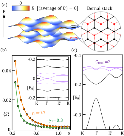
Figure 2: (a) Bernal graphene with vertical buckling and a strain field, giving a periodic psuedomagnetic field $B$ (color map) with zero average. (b) Average overlap deviation between numerical and analytical approximate zero modes with $\eta=0.5$, $\langle S\rangle_{\rm BZ}$, versus $\alpha$ at $\beta=0$. Inset: bandstructure for $(\alpha,\beta,\gamma_{1})=(0.5,0,0.5)$ with low-energy modes $E_{0,1}$ in purple. (c) Bandstructure at $(\alpha,\beta,\gamma_{1})=(0.4,0.068,1)$. Displacement field $\beta>0$ isolates the two low-energy Chern bands (purple).

Periodically Strained Bernal Graphene— We will now show how a first vortexable band appears amongst the low energy bands of periodically strained bilayer graphene [78]. We will take a similar approach to Ref. [79] which studied periodically strained monolayer graphene with a $C_{2}$-breaking substrate that induces $C_{2}$ breaking pseudomagnetic field

$$\mathcal{B}(z,\bar{z})=\mathcal{B}_{0}\sum_{l=0}^{5}e^{i\bm{G}_{l}\cdot\bm{r}}=\mathcal{B}_{0}\sum_{l=0}^{5}e^{\frac{i}{2}\left(G_{l}\bar{z}+\bar{G}_{l}z\right)}$$ (7)

where $\bm{G}_{l}=R_{2\pi l/6}\bm{G}_{0},\bm{G}_{0}=\frac{4\pi}{\sqrt{3}L_{M}}(1,0)$ are smallest reciprocal lattice vectors in terms of the period $L_{M}$; the addition of higher harmonics is not expected to change our conclusions [79]. We note that ${\mathcal{B}}({\bm{r}})={\mathcal{B}}(-{\bm{r}})$, within a valley, implies that the pseudomagnetic field is $C_{2}$-odd. Furthermore, ${\mathcal{B}}(r)$ averages to zero such that the bands we will obtain are Bloch bands, not LLs. The periodic strain can be realized by placing monolayer graphene on a lattice of nanorods [80], or by spontaneous buckling of a graphene sheet on $C_{2}$ breaking substrates such as NbSe2 [81]. We will also include a spatially-varying scalar potential with the same periodicity proportional to $V({\bm{r}})=\sum_{l}e^{i\bm{G}_{l}\cdot{\bm{r}}}$ and of strength $V_{0}$. The scalar potential could come from patterned gates [82, 83, 84, 85, 86], or an electric field that couples to the buckling height.

The (de-dimensionalized) Hamiltonian for AB-stacked graphene’s $K$ valley is then

$$H_{\rm SBG} =E_{0}\left(\begin{array}[]{cc}h&\gamma_{1}\sigma_{+}\\ \gamma_{1}\sigma_{-}&h\end{array}\right),$$ (8)

$$h =\bm{\sigma}\cdot[-i\bm{\nabla}+\alpha\bm{{\mathcal{A}}}]-\beta V({\bm{r}}),$$

where $E_{0}=\hbar v_{F}\lvert\bm{G}_{0}\rvert$, $\sigma_{\pm}=\frac{1}{2}(\sigma_{+}\pm i\sigma_{-})$, $\alpha=1/\ell_{B}^{2}\lvert G_{0}\rvert^{2}$, $\beta=V_{0}/E_{0}$, ${\mathcal{B}}_{0}=\hbar/e\ell_{B}^{2}$, ${\mathcal{A}}=\mathcal{A}_{x}+iA_{y}=\sum_{l}e^{2\pi i/l}e^{i\bm{G}_{l}\cdot\bm{r}}$ We will neglect the interlayer potential for simplicity, consistent with patterned dielectric gates sandwiching the sample.. We take interlayer tunnelling $E_{0}\gamma_{1}\approx 370$ meV and, following  [81], $E_{0}\approx$300\text{\,}\mathrm{m}\mathrm{e}\mathrm{V}$$. The bandstructure, Fig. 2(b) inset, has a low energy subspace of four bands (purple) with total bandwidth $O(e^{-6\alpha})$. In the chiral limit $\beta=0$, $H_{\rm SBG}/E_{0}$ takes the form of Eq. (2) but now with $D_{0}=-2i\overline{\partial}+\alpha{\mathcal{A}}({\bm{r}})$.

We explicitly construct trial wavefunctions on the $A$ sublattice for a zeroth and first vortexable band that — up to exponentially small corrections $O(e^{-6\alpha})$ — are zero modes of $D_{1}$. The two trial wavefunctions are Chern bands whose layer spinors take the form

$$\Phi_{0,\bm{k}}(\bm{r})=\left(\begin{array}[]{c}\psi_{0,\bm{k}}(\bm{r})\\ 0\end{array}\right),\Phi_{1,\bm{k}}(\bm{r})=\left(\begin{array}[]{c}\psi_{1,\bm{k}}(\bm{r})\\ 2i\gamma_{1}^{-1}\psi_{0,\bm{k}}(\bm{r})\end{array}\right),$$ (9)

with precise expressions given in Appendix C. The construction of (9) follows the same reasoning as Ref. [79], making use of $[D_{0},z]=0$ and $\psi_{\Gamma}({\bm{r}}=0)=e^{-6\alpha}\approx 0$, where $V({\bm{r}}=0)=6$. In Appendix C we also construct two topologically trivial near zero modes of $D_{1}^{\dagger}$ for the $B$-sublattice. We now use these trial wavefunctions to identify a first vortexable band of $H_{\mathrm{SBG}}$ and isolate it from the rest of the spectrum.

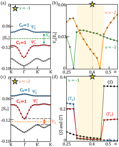
Figure 3: (a),(c): SCHF bandstructures for $\nu=-1$ and $\nu=-2$, respectively, with parameters corresponding to Fig. 2(c), and $(d,\epsilon_{r})=($250\text{\,}\mathrm{\SIUnitSymbolAngstrom}$,15)$. The dashed lines represent the Fermi energy. (b) The band gaps $V_{g}$ for $\nu=-1$ and $\nu=-2$ are plotted with green and orange lines, respectively. (d) Average overlap deviation between numerical and analytical eigenstates with $\eta=0.5$ at $\nu=-1$ as a function of $\alpha$. Here $\langle T_{0}\rangle_{\rm BZ}$ (blue), and $\langle T_{1}\rangle_{\rm BZ}$ (red) correspond to the zeroth and first vortexable bands, whereas $\langle S\rangle_{\rm BZ}$ is tow-band complex.

We now numerically verify that the low-energy subspace of $H_{\mathrm{SBG}}$ on the $A$-sublattice is spanned by the trial wavefunctions Eq.(9) up to $O(e^{-6\alpha})$ corrections. As the energy eigenstates are mixed between the sublattices (at $\beta=0$), they cannot correspond to the trial wavefunctions directly. Instead, we use the sublattice basis $\Psi^{A,B}_{n,{\bm{k}}}=\frac{1}{\sqrt{2}}(\Psi_{E_{n},{\bm{k}}}\pm\sigma_{z}\Psi_{E_{n},{\bm{k}}})$, where $n=0,1$ labels the two eigenstates of smallest $E_{n}>0$, and $\sigma_{z}\Psi_{E_{n}}\propto\Psi_{-E_{n}}$. The overlap deviation between the span of the trial wavefunctions $P_{\Phi{\bm{k}}}=\sum_{n}|\Phi_{n,{\bm{k}}}\rangle\langle\Phi_{n,{\bm{k}}}|$ and the $A$-subspace $P_{\Psi{\bm{k}}}=\sum_{n}|\Psi^{A}_{n,{\bm{k}}}\rangle\langle\Psi^{A}_{n,{\bm{k}}}|$ is quantified by $S_{\bm{k}}[\Phi_{{\bm{k}}},\Psi^{A}_{{\bm{k}}}]=1-\mathrm{Tr}[P_{\Phi{\bm{k}}}P_{\Psi{\bm{k}}}]/2$. The trial wavefunctions span the $A$-subspace if and only if the Brillouin zone average vanishes, $\braket{S}_{\mathrm{BZ}}\approx 0$. Fig. 2(b) shows $\langle S\rangle_{\mathrm{BZ}}$ decreases as $e^{-6\alpha}$, giving overlaps $>0.99$ whenever $\alpha>0.2$. We therefore conclude that the low-energy $A$-sublattice subspace is spanned by “almost" vortexable and first vortexable bands, satisfying the definition up to small $O(e^{-6\alpha})$ corrections.

Finally, we show how interactions can spectrally isolate the almost first-vortexable band. Chiral symmetry is lifted by displacement fields $\beta>0$, breaking the Dirac cone and separating out a complex of two bands $\Psi^{A}_{(0,1)}$ with $C_{\rm total}=2$. The complex’s total bandwidth is minimized at $\beta=0.068$ [Fig 2(c)], but the two bands within it are not isolated without adding interactions. We now add gate-screened Coulomb interactions in the standard way, and study the resulting self-consistent Hartree-Fock (SCHF) bandstructures at integer fillings (details in Appendix H). We find interactions split the complex into two isolated bands $\Psi_{0}^{\prime}$ and $\Psi_{1}^{\prime}$ that approximately are vortexable and first-vortexable, respectively. The overlap deviation $\braket{S}$, shown in Fig. 3(d), decreases as $e^{-5.6\alpha}$. This is directly analogous to Bernal graphene in field, where interactions split the degenerate zeroth and first LLs since the more-concentrated LLL wavefunctions have less exchange energy [87, 88, 89].

Fig. 3 shows SCHF bandstructures at fillings $\nu=-1$ and $-2$, each of which shows two isolated $C=1$ bands. At $\nu=-2$, the SCHF bandgap closes near $\alpha\approx 0.45$, enabling a topological transition $C=(1,1)\to(1,0)$ by mixing with the third band. Conversely, the top two bands hybridize to give isolated bands with $C=(2,0)$ below $\alpha\approx 0.3$. Hence the two $C=1$ bands are isolated over a range of $\alpha$ for both $\nu=-1$ & $-2$.

To confirm vortexability, we compare the numerical wavefunctions to the analytical ansätze $\Phi_{(0,1)}$ from Eq. (9). Fig. 3(d) shows $\langle T_{n}\rangle$, the average of $1-\left|\braket{\Psi_{n{\bm{k}}}^{A}}{\Phi_{n{\bm{k}}}}\right|$ over the BZ and the two band overlap deviation $\langle S\rangle$ defined above. In the regime $0.3<\alpha<0.45$ with $C=(1,1)$, the overlap deviation decreases as $O(e^{-5.6\alpha})$, giving deviations $<1\%$ for $\alpha>0.38$. The numerical wavefunctions therefore match the analytic ones to extremely good precision, and the latter are almost vortexable and first vortexable. We compute the maximality index, Eq. (6), to be $\langle M\rangle_{\rm BZ}\approx 0.79$ at $\alpha=0.4$ and dimensionless tunneling $\gamma_{1}=1$. This is close to the optimal value of $1$.

In this work we have proposed “first vortexability" — a precise definition of when a Chern band has the essential character of the first LL. First vortexable bands are defined by their quantum geometric data, and each requires a partner band analogous to the zeroth LL. Our examples, both analytic and physically reasonable, suggest such bands are experimentally realizable. Future work will investigate the many-body physics of partially-filled first vortexable bands, particularly at half filling where non-Abelian states are likely.

Appendix A Analytic Example at Zero Field

To demonstrate first vortexable bands without magnetic fields, we consider an analytically solvable (albeit artificial) example inspired by chiral twisted bilayer graphene. Let

$$H_{1}=\left(\begin{array}[]{cc}0&D^{\dagger}_{1}\\ D_{1}&0\end{array}\right),\quad D_{1}=\left(\begin{array}[]{cc}D_{0}&\gamma_{1}I_{2\times 2}\\ 0&D_{0}\end{array}\right).$$ (10)

In particular, we assume that $D_{0}$ is the chiral Hamiltonian of twisted bilayer graphene (TBG), given by

$$D_{0}=\left(\begin{array}[]{cc}-2i\bar{\partial}&\alpha U_{\omega^{*}}(\bm{r})\\ \alpha U_{\omega^{*}}(-\bm{r})&-2i\bar{\partial}\end{array}\right),\quad U_{\omega}(\bm{r})=\alpha\sum_{j=0}^{2}\omega^{j}e^{-i\bm{q}_{j}\cdot\bm{r}}$$ (11)

with $\omega=e^{2\pi i/3}$ and $q_{j,x}+iq_{j,y}=-ie^{2\pi j/3}$. While (10) may appear strange due to the upper triangular hoppings connecting non-nearest-“layers", after a suitable unitary transformation it arises exactly as a $k_{z}=0$ band of three dimensional twisted AB-BA double bilayer graphene (see Sec B). At each magic angle (such as $\alpha\approx 0.586$), $D_{0}$ has a zero mode [73, 19, 90]

$$\psi_{0,{\bm{k}}}(r)=\frac{\sigma\left(z+iB_{0}^{-1}k\right)}{\sigma(z)}e^{\frac{i}{2}\bar{k}z}\psi_{\Gamma}({\bm{r}}),$$ (12)

where $\sigma(z)$ is the Weierstrass $\sigma$-function [91, 90]. The Weierstrass sigma function $\sigma(z)$ satisfies $\sigma(-z)=-\sigma(z)$ and $\sigma(z+R)=\eta_{\bm{r}}e^{\frac{B}{2}\bar{R}(z+R/2)}\sigma(z)$, where $\eta_{\bm{R}}=+1$ if $\bm{R}/2$ is a lattice vector and $-1$ otherwise.

We can now construct $\Phi_{0,\bm{k}}=\big{[}\psi_{0,\bm{k}},0\big{]}^{T}$ and $\Phi_{1,\bm{k}}=\big{[}\psi_{1,\bm{k}},2i\gamma_{1}^{-1}\psi_{0,\bm{k}}\big{]}^{T}$, where

$$\psi_{1,{\bm{k}}}(\bm{r})=\left[\bar{z}-\frac{2B_{0}^{-1}\partial_{z}\sigma\left(z+iB_{0}^{-1}k\right)}{\sigma\left(z+iB_{0}^{-1}k\right)}-\alpha({\bm{k}})\right]\psi_{0,{\bm{k}}}(\bm{r}).$$ (13)

with $\alpha({\bm{k}})$ such that $\braket{\psi_{0,{\bm{k}}}}{\psi_{1,{\bm{k}}}}=0$. Then the identity $D_{0}\psi_{1,{\bm{k}}}=-\psi_{0,{\bm{k}}}$ immediately implies $D_{1}\Phi_{1,\bm{k}}=0$, giving two bands of zero modes analogous to the LLL and 1LL. We note $\psi_{1,{\bm{k}}}$ obeys the Bloch condition because the shift in $z\rightarrow z+R$ in the first term is cancelled out by

$$\partial_{z}\sigma(z+R)=-e^{\frac{B_{0}}{2}\bar{R}(z+R/2)}\left[\partial_{z}\sigma(z)-\frac{B_{0}}{2}\bar{R}\sigma(z)\right].$$ (14)

We numerically confirm that $\Phi_{0}$ and $\Phi_{1}$ are the zero-modes of $H_{1}$ [Eq. (10)] at the magic angle of TBG. There $H_{1}$ has four low-energy bands isolated from the remote bands, whose bandwidth vanishes at the same magic angle as TBG, $\alpha=0.586$ [Fig. 5(b)]. Due to the chiral symmetry of the Hamiltonian, the four eigenstates, denoted by $\Psi_{\pm E_{n}}$ with the energy $E_{n}>0$ $(n=0,1)$, can be decomposed into sublattice polarized states such as $\Psi_{n\bm{k}}^{A,B}=\frac{1}{\sqrt{2}}\left(\Psi_{E_{n},{\bm{k}}}\pm\sigma_{z}\Psi_{E_{n},{\bm{k}}}\right)$. In Fig. 5(b), we plot the bandwidth and the average of $1-\left|\braket{\Psi_{n{\bm{k}}}^{A}}{\Phi_{n{\bm{k}}}}\right|$ over the BZ, denoted by $\langle T_{n}\rangle_{\rm BZ}$. At the magic angle $\Psi_{n\bm{k}}^{A}=\Phi_{n{\bm{k}}}$ exactly, as expected.

Appendix B Three dimensional twisted AB-BA double bilayer

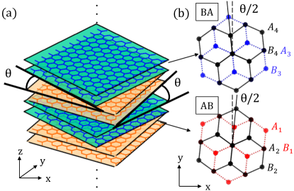
Figure 4: Schematic picture of three-dimensional alternatively ABBA twisted Bernal graphene.

The Hamiltonian [Eq.(10)] corresponds to the model where the layers are twisted by $(0,\theta,\theta,2\theta)$ and hosts a hopping between different sublattices of the next nearest layers. Using the unitary transformation such as changing the order of layer basis $(|\sigma,1\rangle,|\sigma,2\rangle,|\sigma,3\rangle,|\sigma,4\rangle)$ into $(|\sigma,1\rangle,|\sigma,3\rangle,|\sigma,4\rangle,|\sigma,2\rangle)$, where $\sigma=\pm$ denotes $A/B$, we obtain the following Hamiltonian

$$\mathcal{H}_{\rm{3DATDBG}}=\mathcal{H}_{\rm{AB-BA}}+\left(\begin{array}[]{cccc}0&0&0&T^{\dagger}(\bm{r})\\ 0&0&0&0\\ 0&0&0&0\\ T(\bm{r})&0&0&0\end{array}\right).$$ (15)

where the first term is the Hamiltonian of twisted AB-BA double bilayer (TDBG) [92]

$$\mathcal{H}_{\rm{AB-BA}}=\left(\begin{array}[]{cccc}-i\bm{\sigma}\cdot\bm{\nabla}&\Gamma_{1}^{\dagger}&0&0\\ \Gamma_{1}&-i\bm{\sigma}\cdot\bm{\nabla}&T^{\dagger}(\bm{r})&0\\ 0&T(\bm{r})&-i\bm{\sigma}\cdot\bm{\nabla}&\Gamma_{1}\\ 0&0&\Gamma_{1}^{\dagger}&-i\bm{\sigma}\cdot\bm{\nabla}\end{array}\right)$$ (16)

with $\Gamma_{1}=(\sigma_{x}-i\sigma_{y})\gamma_{1}/2$.

$$T(\bm{r})=\sum_{n=1}^{3}T_{n}e^{-i\bm{q}_{n}\cdot\bm{r}}$$ (17)

where $T_{n+1}=\alpha\left(\sigma_{x}\cos n\phi+\sigma_{y}\sin n\phi\right)$ is the interlayer hopping in the chiral limit. The second term is the interlayer coupling between layer 1 and 4, implying imposing the periodic boundary condition to the twisted AB-BA double bilayer in the stacking direction. This model can be realized in three-dimensional alternatively twisted AB-BA double bilayer graphene shown in Fig. 4. In an infinite number of stackings of TDBG, the wavenumber $k_{z}$ along the stacking direction is a good quantum number to label the energy state. At $k_{z}=0$, the Hamiltonian is equivalent to Eq.(15).

Appendix C Trial wavefunction of zeroth and first vortexable state of strained Bernal graphene

Let us construct the trial wavefunction of zeroth and first vortexable state of strained Bernal graphene. At $\beta=0$ the chiral symmetry of the model allows us to write

$$H_{\rm SBG} =E_{0}\begin{pmatrix}0&D_{1}^{\dagger}\\ D_{1}&0\end{pmatrix},\,\,\,D_{1}=\begin{pmatrix}D_{0}&\gamma_{1}\\ 0&D_{0}\end{pmatrix}$$ (18)

$$D_{0} =-2i\overline{\partial}+\alpha{\mathcal{A}}.$$

We will obtain the low energy subspace through sublattice polarized near-zero modes of $D_{1}$ and $D_{1}^{\dagger}$. We will begin with $D_{1}$. At the $\Gamma$ point, there is an exact zero mode of $D_{0}$, $\psi_{0,\Gamma}({\bm{r}})=e^{-\alpha V({\bm{r}})}$, and an associated zero mode of $D_{1}$ (and thus $H$) by placing $\psi_{0,\Gamma}$ in the top layer component. We now create two near zero modes, for large $\alpha$, under the approximation $\psi_{0,\Gamma}({\bm{r}}=0)=e^{-6\alpha}\approx 0$; where here and below “$\approx$" specifically means “up to terms of $O\left(e^{-6\alpha}\right)"$.

We begin by constructing an approximate zero mode of $D_{0}$, following Ref. [79]. We will use the modified state $\psi_{\eta}=f_{\eta}({\bm{r}})e^{-\alpha V({\bm{r}})}$, where $f_{\eta}({\bm{r}})=0$ near ${\bm{r}}=0$ but is $1$ otherwise (e.g. $f_{\eta}({\bm{r}})=\tanh\eta\lvert{\bm{r}}\rvert$ for $\eta\gg 1$). Then, $D_{0}\psi_{\eta}\approx 0$. Furthermore, since $\psi_{\eta}({\bm{r}}=0)=0$ by construction, we have

$$D_{0}\mathcal{N}({\bm{r}})=0,\qquad\mathcal{N}({\bm{r}})=\frac{\psi_{\eta}({\bm{r}})}{\sigma(z)}$$ (19)

where $\sigma(z)$ is the Weierstrass $\sigma$-function [91, 90, 79] that we used in Sec. A; see the discussion below (12). Since $\lvert\sigma(z)\rvert^{-1}$ decreases exponentially as $\lvert z\rvert\to\infty$, like the usual Gaussian factor of the LLL, we can now multiply by holomorphic functions, that necessarily blow up at infinity, and thereby construct a vortexable band $\psi_{0}=f(z)\mathcal{N}({\bm{r}})$.

These wavefunctions satisfy $D_{0}\psi_{0}\approx 0$ by construction. To construct Bloch states we write

$$\psi_{0,{\bm{k}}}({\bm{r}}) =f_{\bm{k}}(z)\mathcal{N}_{0}({\bm{r}})$$ (20)

$$f_{\bm{k}}(z) =e^{\frac{i}{2}\overline{k}z}\sigma(z+iB_{0}^{-1}k).$$

The construction (20) directly yields an approximate zero mode of $D_{1}$, by placing $\psi_{0,{\bm{k}}}({\bm{r}})$ in the top component, analogously to the zeroth LL of $B>0$ Bernal graphene and the analytical zero field model of the previous section. To obtain the second approximate zero mode, we write

$$\psi_{1,{\bm{k}}}({\bm{r}})=Q_{\psi_{0}}(\overline{z}f_{\bm{k}}(z)-2B_{0}^{-1}\partial_{z}f_{\bm{k}}(z))\mathcal{N}({\bm{r}})$$ (21)

, $Q_{\psi_{0}}$ projects out the component proportional to $\psi_{0,{\bm{k}}}$. Since $D_{0}\psi_{0,{\bm{k}}}\approx 0$ and $D_{0}\psi_{1,{\bm{k}}}\approx-\psi_{0,{\bm{k}}}$, the states

$$\Phi_{0,\bm{k}}(\bm{r})=\left(\begin{array}[]{c}\psi_{0,\bm{k}}(\bm{r})\\ 0\end{array}\right),\Phi_{1,\bm{k}}(\bm{r})=\left(\begin{array}[]{c}\psi_{1,\bm{k}}(\bm{r})\\ 2i\gamma_{1}^{-1}\psi_{0,\bm{k}}(\bm{r})\end{array}\right),$$ (22)

satisfy $D_{1}\Phi_{(0,1),\bm{k}}(\bm{r})\approx 0$, giving two almost flat bands of zero modes analogous to the LLL and 1LL. We may also write them in the general form we quoted for zeroth and first vortexable bands,

$$\Phi_{0,\bm{k}}(\bm{r}) =f_{{\bm{k}}}(z)\mathcal{N}_{0}({\bm{r}})$$ (23)

$$\Phi_{0,\bm{k}}(\bm{r}) =Q_{\psi_{0}}\left[(\overline{z}f_{\bm{k}}(z)-2B_{0}^{-1}\partial_{z}f_{\bm{k}}(z))\mathcal{N}_{0}({\bm{r}})+f_{\bm{k}}(z)\mathcal{N}_{1}({\bm{r}})\right],$$

where

$$\mathcal{N}_{0}({\bm{r}})=\begin{pmatrix}1\\ 0\end{pmatrix},\quad\mathcal{N}_{1}({\bm{r}})=\begin{pmatrix}0\\ 2i\gamma_{1}^{-1}\end{pmatrix}.$$ (24)

The two $B$-sublattice zero modes of $D_{1}^{\dagger}$ are topologically trivial. The exact zero mode of $D_{0}$, $\chi_{0,\Gamma}=e^{+\alpha V}$, is strongly localized at a single site ${\bm{r}}={\bm{R}}$ in each unit cell centered at the lattice vector ${\bm{R}}$. Let us define $\chi_{0,{\bm{R}}}({\bm{r}})$ to be equal to $\chi_{\Gamma}({\bm{r}})$ if ${\bm{r}}$ is in the unit cell centered at ${\bm{R}}$, and zero otherwise. It is exponentially localized around ${\bm{r}}={\bm{R}}$, and satisfies $D_{0}=\chi_{0,{\bm{R}}}({\bm{r}})\approx 0$ as well; it should be thought of as a Wannier state of the strained monolayer. Now we construct

$$\mathcal{X}_{0,{\bm{R}}}({\bm{r}})=\begin{pmatrix}\chi_{0,{\bm{R}}}({\bm{r}})\\ 0\end{pmatrix},\quad\mathcal{X}_{1,{\bm{R}}}({\bm{r}})=\begin{pmatrix}z\chi_{0,{\bm{R}}}({\bm{r}})\\ 2i\gamma^{-1}\chi_{0,{\bm{R}}}({\bm{r}})\end{pmatrix},$$ (25)

as exponentially localized Wannier states at each site which satisfy $D_{1}\mathcal{X}_{0,1{\bm{R}}}({\bm{r}})\approx 0$.

Appendix D Multi-band Vortexable Band Geometry

In this section we review ideal, or vortexable, band geometry for multiple bands and study the non-Abelian quantum geometric tensor in this context for later use. The non-Abelian quantum geometric tensor (QGT) is given, in an orthonormal basis, as

$$\hat{\eta}^{\mu\nu}_{ab} =\bra{\partial_{k_{\nu}}u_{{\bm{k}}b}}Q({\bm{k}})\ket{\partial_{k_{\mu}}u_{{\bm{k}}a}},$$ (26)

$$Q({\bm{k}}) =1-\sum_{a}\ket{u_{{\bm{k}}a}}\bra{u_{{\bm{k}}a}}$$

where $a,b$ are band-indices.

We will denote its trace by removing its hat, or with a capital $\operatorname{Tr}$, i.e.

$$\eta^{\mu\nu}=\operatorname{Tr}\hat{\eta}^{\mu\nu}=\sum_{a}\eta^{\mu\nu}_{aa}.$$ (27)

Note that our gauge-covariance based definition of $\hat{\eta}$ ensures that $\eta^{\mu\nu}$ is gauge invariant, even in non-orthonormal bases. The non-Abelian Berry curvature and metric are defined with the symmetric and antisymmetric components in the spatial indices

$$\begin{aligned} \hat{g}^{\mu\nu}({\bm{k}})&=\frac{1}{2}(\hat{\eta}^{\mu\nu}+\hat{\eta}^{\nu\mu})\\ \hat{\Omega}_{ab}\varepsilon^{\mu\nu}&=i(\hat{\eta}^{\mu\nu}-\hat{\eta}^{\nu\mu})\end{aligned}.$$ (28)

We now claim the following conditions are equivalent [28, 22, 21, 23, 24]

1. The bands are vortexable: $z\psi=Pz\psi$, where $\psi=P\psi$ is any wavefunction in the band and $P$ is the band projector.

2. The inequality $\operatorname{tr}g\geq\Omega$, or $\operatorname{tr}\operatorname{Tr}\hat{g}\geq\operatorname{Tr}\hat{\Omega}$, is saturated, where $z+x+iy$ is the vortex function.

3. There is a gauge, in which the wavefunctions are generically non-orthonormal, such that $\ket{u_{{\bm{k}}a}}=\ket{u_{ka}}$ are holomorphic functions of $k=k_{x}+ik_{y}$.

4. The quantum metric factorizes as $\hat{\eta}^{\mu\nu}_{ab}=\frac{1}{2}\hat{\Omega}_{ab}(\delta_{\mu\nu}-i\varepsilon_{\mu\nu})$, where $\hat{\Omega}_{ab}=\bra{\partial_{k}u_{{\bm{k}}b}}Q({\bm{k}})\ket{\partial_{k}u_{{\bm{k}}a}}$ is the non-Abelian Berry curvature and $2\partial_{k}=\partial_{k_{x}}+i\partial_{k_{y}}$ is the derivative with respect to $k=k_{x}+ik_{y}$

Ref. [28] showed the equivalence between (V1) and (V2), and reviewed the equivalence between (V2) and (V3) through an explicit construction of the required gauge transformation, which was previously shown to exist by Ref. [22]. It remains to show (V4) is equivalent to (V1-3). The implication $\rm{(V4)}\implies\rm{(V2)}$ follows immediately by computing $\operatorname{tr}g$ and $\Omega$ from the traced symmetric and antisymmetric parts of $\hat{\eta}^{\mu\nu}_{ab}=\frac{1}{2}\hat{\Omega}_{ab}(\delta_{\mu\nu}-i\varepsilon_{\mu\nu})$ respectively. We conclude by showing $\rm{(V3)}\implies\rm{(V4)}$; to see this, we use $(V3)$ to write $\ket{u_{{\bm{k}}}}=S_{\bm{k}}\ket{\tilde{u}_{k}}$, where $S_{\bm{k}}$ is a matrix that is not necessarily unitary and $\ket{\tilde{u}_{k}}$ is holomorphic. Then we have

$$Q({\bm{k}})\partial_{k_{x}}\ket{u_{{\bm{k}}a}} =Q({\bm{k}})(\partial_{k}+\overline{\partial}_{k})S_{\bm{k}}\ket{\tilde{u}_{k}}$$ (29)

$$=S_{\bm{k}}Q({\bm{k}})\partial_{k}\ket{\tilde{u}_{ka}}$$

$$=Q({\bm{k}})\partial_{k}\ket{u_{{\bm{k}}a}}$$

where we used that the term coming from differentiating $S({\bm{k}})$ is annihilated by $Q({\bm{k}})$. Similarly we can write $Q({\bm{k}})\partial_{k_{y}}\ket{u_{{\bm{k}}}}=iQ({\bm{k}})\partial_{k}\ket{u_{{\bm{k}}}}$. Substituting into (27) then yields (V4).

Appendix E First vortexability of trial wavefunctions

In this section we show explicitly that the trial wavefunctions that we have used throughout the main text are first vortexable. For readability, we recall the definition now. A band is first vortexable if

1. The band is not vortexable by itself

2. There exists an orthogonal vortexable band with projector $P_{0}$ (i.e. $P_{0}z\psi_{0}~{}=~{}z\psi_{0}$ for all $P_{0}\psi_{0}=\psi_{0}$) such that

   $$(P_{1}+P_{0})z\psi_{1}=z\psi_{1}$$ (30)

   for all states $P\psi_{1}=\psi_{1}$

3. There is no alternative basis of wavefunctions $(\phi_{0,{\bm{k}}},\phi_{1,{\bm{k}}})$, where each band is vortexable, that also spans the two band subspace $P_{0}+P_{1}$

We begin with a useful Lemma used repeatedly below.

Lemma 1.

A function of crystal momentum that satisfies $f({\bm{k}}+{\bm{G}})=f({\bm{k}})-i\lambda\overline{G}$ under translation by reciprocal lattice vectors, for some $\lambda\neq 0$, is not holomorphic in $k_{x}+ik_{y}$.

Proof.

Consider a contour integral of $f$ around the parallelogram boundary of the BZ, with side lengths $G_{1}$ and $G_{2}$, that vanishes for holomorphic functions by Cauchy’s theorem. On the other hand, the shift-periodicity of $f$ relates the integrals on opposite sides of the parallelogram such that

$$\oint_{\partial{\mathrm{BZ}}}f({\bm{k}})dk=-i\lambda(\overline{G_{1}}G_{2}-\overline{G_{2}}G_{1})=\lambda A_{\mathrm{BZ}}\neq 0.$$ (31)

We conclude that $f$ is not holomorphic ∎

We begin by outlining how we will show that the trial wavefunctions $(\Phi_{0,{\bm{k}}},\Phi_{1,{\bm{k}}})$ used in the main text are vortexable and first vortexable, respectively. The first step is to show that the various $\Phi_{1,{\bm{k}}}({\bm{r}})$ we have constructed are not vortexable themselves, property (P2) but are when combined with $\Phi_{0,{\bm{k}}}({\bm{r}})$, (P1). It is possible to show this in real space, by acting with $z$ on $\Phi_{1,{\bm{k}}}({\bm{r}})$ and expressing the result as a sum of $\Phi_{1,{\bm{k}}}({\bm{r}})$ and $\Phi_{0,{\bm{k}}}({\bm{r}})$. However, (P3) demands that is no “decomposed" basis, in which the space spanned by $\Phi_{(0,1){\bm{k}}}({\bm{r}})$ is split into two bands that are vortexable on their own. To show that such a basis doesn’t exist, it is convenient to work in a holomorphic gauge in momentum space as there are powerful no-go results on holomorphic functions. Thus, throughout this section we will use the equivalence of vortexability with the existence of a holomorphic gauge (V3). We note that the wavefunctions in the holomorphic gauge are generically neither normalized nor orthogonal, and gauge transformations are invertible but generically non-unitary.

We note that all trial wavefunctions that we have used (c.f. Secs. A and C) have periodic wavefunctions $u_{\bm{k}}({\bm{r}})=e^{-i{\bm{k}}\cdot{\bm{r}}}\Phi_{\bm{k}}({\bm{r}})$ of the form

$$u_{0,k}({\bm{r}}) =f_{k}(z)\mathcal{N}_{0}({\bm{r}})$$ (32)

$$u_{1,{\bm{k}}}({\bm{r}}) =\left[\left(\overline{z}-2B_{0}^{-1}\partial_{z}-\alpha({\bm{k}})\right)f_{k}({\bm{r}})\right]\mathcal{N}_{0}({\bm{r}})$$

$$+f_{k}({\bm{r}})\mathcal{N}_{1}({\bm{r}})$$

where

$$f_{k}({\bm{r}})=e^{-\frac{i}{2}k\overline{z}}\sigma(z+iB_{0}^{-1}k).$$ (33)

We have used that multiplication by $e^{i{\bm{k}}\cdot{\bm{r}}}$ converts $e^{\frac{i}{2}\overline{k}z}$ to $e^{-\frac{i}{2}k\overline{z}}$. The function $\alpha({\bm{k}})$ was chosen so that the states are orthogonal, and the functions $\mathcal{N}_{0,1}^{l}({\bm{r}})$ are functions of the layer and real-space but not ${\bm{k}}$. We note that we can write $\left(\overline{z}-2B_{0}^{-1}\partial_{z}\right)f_{k}({\bm{r}})=2i\partial_{k}f_{k}({\bm{r}})$. This implies that we can form the $k$-holomorphic states

$$v_{0,k}=u_{0,k},\,\,v_{1,k}({\bm{r}})=2i\partial_{k}u_{0,k}({\bm{r}})+f_{k}({\bm{r}})\mathcal{N}_{1}({\bm{r}})$$ (34)

as an alternative holomorphic basis through dropping $\alpha({\bm{k}})$.

It is important to emphasize that the wavefunctions $v_{1,k}^{l}({\bm{r}})$ do not describe a vortexable band despite the fact that they are holomorphic in $k$. Indeed, they do not define a single Bloch band because $v_{1,k+G}$ is not proportional to $v_{1,k}$. Using $\sigma(z+R)=\eta_{\bm{R}}e^{\frac{B}{2}\bar{R}(z+R/2)}\sigma(z)$, we have that

$$v_{0,k+G}({\bm{r}})=e^{-i{\bm{G}}\cdot{\bm{r}}}\xi_{\bm{G}}(k)v_{0,k}({\bm{r}})$$

for $\xi_{G}(k)=\eta_{\bm{G}}e^{\frac{1}{2}B^{-1}\overline{G}(k+\frac{G}{2})}$. In contrast,

$$v_{1,k+G}({\bm{r}}) =e^{-i{\bm{G}}\cdot{\bm{r}}}\left(2i\partial_{k}(\xi_{{\bm{G}}}(k)v_{0,k}+\xi_{{\bm{G}}}(k)f_{k}({\bm{r}})\mathcal{N}_{1}\right)$$ (35)

$$=e^{-i{\bm{G}}\cdot{\bm{r}}}\xi_{{\bm{G}}}(k)(v_{1,k}+iB_{0}^{-1}\overline{G}v_{0,k})$$

where we used $2i\xi_{\bm{G}}^{-1}\partial_{k}\xi_{\bm{G}}=iB_{0}^{-1}\overline{G}$.

The existence of the above holomorphic gauge shows that the entire two band subspace is vortexable, (P2). However, the nonperiodicity allows us to show that $u_{1,{\bm{k}}}=v_{1,k}({\bm{r}})-\alpha({\bm{k}})v_{0,k}({\bm{r}})$ is not vortexable on its own. Indeed, $v_{1,k}$ is vortexable if and only if $\alpha({\bm{k}})$ is holomorphic. However, using boundary conditions for $v_{nk}$, we find $\alpha({\bm{k}})=\lVert v_{0,k}\rVert^{-2}\braket{v_{0,k}}{v_{1,k}}$ satisfies $\alpha({\bm{k}}+{\bm{G}})=\alpha({\bm{k}})+iB_{0}^{-1}\overline{G}$. Thus Lemma 1 implies $\alpha$ is not holomorphic, and (P1) is satisfied.

We must now prove (P3). This amounts to showing that

$$\begin{pmatrix}w_{0,k}\\ w_{1,k}\end{pmatrix}=S_{k}^{-1}\begin{pmatrix}v_{0,k}\\ v_{1,k}\end{pmatrix}$$ (36)

cannot have diagonal boundary conditions,

$$\begin{pmatrix}w_{0,k+G}\\ w_{1,k+G}\end{pmatrix}=e^{-i{\bm{G}}\cdot{\bm{r}}}\begin{pmatrix}\tilde{\xi}_{\bm{G}}^{(0)}(k)&0\\ 0&\tilde{\xi}_{\bm{G}}^{(1)}(k)\end{pmatrix}\begin{pmatrix}w_{0,k}\\ w_{1,k}\end{pmatrix},$$ (37)

for any holomorphic invertible matrix $S_{k}$.

Our strategy will be to assume diagonal boundary conditions (37) and holomorphic $S_{k}$ and seek a contradiction. The boundary conditions of $v_{mk}$ that we computed above, phrased in matrix notation, are

$$\begin{pmatrix}v_{0,k+G}\vspace{0.5em}\\ v_{1,k+G}\end{pmatrix}=e^{-i{\bm{G}}\cdot{\bm{r}}}\xi_{G}(k)\begin{pmatrix}1&0\\ iB_{0}^{-1}\overline{G}&1\end{pmatrix}\begin{pmatrix}v_{0,k}\vspace{0.5em}\\ v_{1,k}\end{pmatrix}.$$ (38)

The boundary conditions for $w_{k}$ are then related to the gauge transformation $S_{k}$ as

$$S_{k+G}\begin{pmatrix}\tilde{\xi}_{\bm{G}}^{(0)}(k)&0\\ 0&\tilde{\xi}_{\bm{G}}^{(1)}(k)\end{pmatrix}=\xi_{\bm{G}}(k)\begin{pmatrix}1&0\\ i\overline{G}&1\end{pmatrix}S_{k}.$$ (39)

We first focus on the top left entry of (39), which reads

$$S_{00}(k+G)\tilde{\xi}_{{\bm{G}}}^{(0)}(k)=S_{00}(k)\xi_{\bm{G}}(k),$$ (40)

where $S_{00}$ is the top left entry of $S$. Without loss of generality assume that the Chern number $C_{0}$ of the band described by $w^{0,k}$ is zero or one (the Chern numbers must sum to two, and the Chern numbers of vortexable bands are positive). If $C_{0}=0$, then the band admits a tight-binding description with one delta-function-localized Wannier state per unit cell [28] and thus a gauge with $w_{0,k}=1$, and $\tilde{\xi}^{(0)}_{{\bm{G}}}(k)=1$. Since $S_{k}$ is invertible, we can demand that $h(k)=\partial_{k}\log S_{00}(k)$ is holomorphic. However, by (40), with $\tilde{\xi}^{(0)}_{{\bm{G}}}(k)=1$, we have $h(k+G)=h(k)+\frac{1}{2}\overline{G}$, so that by Lemma 1 $h(k)$ is not holomorphic. We therefore rule out the $C_{0}=0$ case, and focus on $C_{0}=1$.

Vortexable bands with $C_{0}=1$ have been classified [23, 26], and have boundary conditions $\tilde{\xi}_{\bm{G}}^{(0)}(k)=\eta_{\bm{G}}e^{\frac{1}{2}B^{-1}\overline{G}(k-k_{0}+\frac{G}{2})}=\xi_{\bm{G}}(k-k_{0})$, for some offset $k_{0}$. Then, Lemma 1 applied to $\log S_{00}(k)$ this time implies $k_{0}=0$, so that $S_{00}(k+G)=S_{00}(k)$ is periodic. Periodic holomorphic functions are constant, so we can set $S_{00}(k)=1$ without loss of generality. The lower-left component of (39) then yields $S_{10}(k+G)=S_{10}(k)+iB_{0}^{-1}\overline{G}$, which again leads to a contradiction by Lemma 1. We have thus proven (P3), so that we can conclude that the trial wavefunctions used in the main text are first vortexable.

Appendix F QGT of “maximal" first vortexability

In this section, we compute the quantum geometric tensor of the combined space of a “maximal" first vortexable band and its zeroth counterpart. By maximal, we specifically mean that there is no zeroth LL portion in the wavefunction other than what is required for the orthogonal basis. For example, in the language of the holomorphic periodic states of the previous section,

$$v_{kl}^{(0)} =f_{k}({\bm{r}})\mathcal{N}_{0}({\bm{r}}),$$ (41)

$$v_{kl}^{(1)} =2i\partial_{k}f_{k}({\bm{r}})\mathcal{N}_{0}({\bm{r}})+f_{k}({\bm{r}})\mathcal{N}_{1}({\bm{r}}),$$

we demand $\mathcal{N}_{1}({\bm{r}})\to 0$. This corresponds to the limit $\gamma_{1}\ell_{B}/v\to\infty$ in the Bernal graphene based Hamiltonians in the main text. In an orthonormal basis we then obtain

$$u_{0,{\bm{k}}} =\frac{1}{N_{0,{\bm{k}}}}f_{k}({\bm{r}})\mathcal{N}_{0}({\bm{r}}),$$ (42)

$$u_{1,{\bm{k}}} =\frac{1}{N_{1,{\bm{k}}}}Q_{0}({\bm{k}})\partial_{k}u_{0,{\bm{k}}}$$

where $Q_{0}({\bm{k}})=1-\ket{u_{0,k}}\bra{u_{0,k}}$ orthogonalizes $u_{1,k}$ relative to $u_{0,k}$ and the factors $N_{m,{\bm{k}}}$ are such that the wavefunctions are normalized.

We recall property (V4), which states that vortexability of the bands is equivalent to $\hat{\eta}^{\mu\nu}_{ab}=\frac{1}{2}\hat{\Omega}_{ab}(\delta_{\mu\nu}-i\varepsilon_{\mu\nu})$, where the Berry curvature is

$$\hat{\Omega}_{ab}({\bm{k}})=\bra{\partial_{k}u_{{\bm{k}}b}}Q({\bm{k}})\ket{\partial_{k}u_{{\bm{k}}a}}$$ (43)

We now show that $\hat{\Omega}_{00}=\hat{\Omega}_{01}=\hat{\Omega}_{10}=0$, in the maximal $\mathcal{N}^{(1)}\to 0$ limit, so that the only nonzero entry is $\hat{\Omega}_{11}$, as claimed in the main text.

From (43), it sufficies to show $Q({\bm{k}})\ket{\partial_{k}u_{0,{\bm{k}}}}=0$. This in turn follows from writing

$$\ket{\partial_{k}u_{0,{\bm{k}}}} =P_{0}\ket{\partial_{k}u_{0,{\bm{k}}}}+Q_{0}\ket{\partial_{k}u_{0,{\bm{k}}}},$$ (44)

$$=P_{0}\ket{\partial_{k}u_{0,{\bm{k}}}}+N_{1,{\bm{k}}}\ket{u_{1,{\bm{k}}}},$$

where we used (42). The first term is proportional to $u_{0,{\bm{k}}}$ by construction while the second term is proportional to $u_{1,{\bm{k}}}$, so that $Q({\bm{k}})\ket{\partial_{k}u_{0,{\bm{k}}}}=0$ as claimed.

Appendix G $\gamma_{1}$ dependence for $M(\mathbf{k})$

Figure 5: (a)$\langle M\rangle_{\rm BZ}$ for the analytical example [Eq.(10)] (green points) and Bernal graphene with magnetic field [Eq.(53)] (black line) as a function of $\gamma_{1}$, and $\gamma_{1}\ell_{B}/\sqrt{2}v$, respectively. (b) The gray line represents the bandwidth of the set of four low-energy bands of Eq.(10) as a function of $\alpha$ for $\gamma_{1}=1$. The bandwidth becomes zero at the magic angle of TBG, $\alpha=0.586$. The blue and red lines are the averaged overlaps $\langle T_{n}\rangle_{\rm BZ}$ for $n=0$ and $n=1$, respectively.

In this section, we compute the “maximality index" which measures how close one is to the “maximal" first LL:

$$M({\bm{k}})=\frac{\lvert\lambda_{1}({\bm{k}})-\lambda_{2}({\bm{k}})\rvert}{\lambda_{1}({\bm{k}})+\lambda_{2}({\bm{k}})},$$ (45)

where $\lambda_{1,2}$ are the eigenvalues of the $2\times 2$ non-Abelian Berry curvature. The previous subsection implies $M({\bm{k}})=1$ when $\mathcal{N}_{1}\to 0$. Here we will compute $M$ for Bernal graphene with constant $B>0$ analytically. We will also discuss the $M({\bm{k}})$ of the chiral TBG example, which ends up closely related.

Bernal graphene in an external magnetic field has a continuous magnetic translation symmetry; the magnetic translation operators are $T(\bm{l})=e^{-i\xi_{\bm{l}}(\bm{r})}t(\bm{l})$ where $t(\bm{l})=e^{i\bm{l}\cdot\bm{\nabla}}$ is the ordinary, $B=0$ translation operator. The phase satisfies $\bm{A}(\bm{r}+\bm{l})=\bm{A}(\bm{r})+\nabla\xi_{\bm{l}}(\bm{r})$, where $\bm{A}$ is the vector potential. The magnetic translation operators satisfy

$$T(\bm{l}_{1})T(\bm{l}_{2})=T(\bm{l}_{2})T(\bm{l}_{1})e^{iB\hat{z}\cdot\bm{l}_{1}\times\bm{l}_{2}}$$ (46)

A commuting subset, generated by $T_{{\bm{R}}_{1}}$, $T_{{\bm{R}}_{2}}$ with $B\hat{z}\cdot{\bm{R}}_{1}\times{\bm{R}}_{2}=2\pi$, can then be used to define Bloch states $\Phi_{{\bm{k}}}({\bm{r}})$. The algebra (46) implies that magnetic translations at other $\ell\neq{\bm{R}}$ act as “ladder operators" on the Bloch states, $T_{\bm{l}}\Phi_{{\bm{k}}}\propto\Phi_{{\bm{k}}-B\hat{z}\times\bm{l}}$ (see e.g. Appendix B of Ref. [26] for a pedagogical discussion). Thus, all Bloch momenta are symmetry related. We will shortly use this fact to specialize to calculating the Berry curvature at ${\bm{k}}=0$.

The periodic states $\mathcal{U}_{m,{\bm{k}}}=e^{-i{\bm{k}}\cdot{\bm{r}}}\Phi_{m,{\bm{k}}}({\bm{r}})$ of Bernal graphene have the form

$$\mathcal{U}_{0,{\bm{k}}} =\left(\begin{array}[]{c}u_{0,{\bm{k}}}\\ 0\end{array}\right),$$ (47)

$$\mathcal{U}_{1,{\bm{k}}} =\frac{1}{\sqrt{\gamma_{1}^{2}+2(v\ell_{B}^{-1})^{2}}}\left(\begin{array}[]{c}\gamma_{1}u_{1,{\bm{k}}}\\ \sqrt{2}v\ell_{B}^{-1}u_{0,{\bm{k}}}\end{array}\right),$$

where $u_{0,{\bm{k}}}$ is the periodic state of the usual LLL and $u_{1,{\bm{k}}}$ is that of the usual first LL, obtained from the lowest through the raising operator. Both states are normalized. We will shortly use

$$u_{1,{\bm{k}}}=\sqrt{B}Q_{0}({\bm{k}})\partial_{k}u_{0,{\bm{k}}}$$ (48)

which can be computed directly or indirectly. The indirect route begins by writing $u_{1,{\bm{k}}}=\lambda Q_{0}({\bm{k}})\partial_{k}u_{0k}$. One then solves for $\lambda=\sqrt{B}$ through $1=\braket{u_{1,{\bm{k}}}}{u_{1,{\bm{k}}}}=\lvert\lambda\rvert^{2}\bra{\partial_{k}u_{0,{\bm{k}}}}Q({\bm{k}})\ket{\partial_{k}u_{0,{\bm{k}}}}=\lvert\lambda\rvert^{2}\Omega_{\text{LLL}}$, where we have identified $\Omega_{\text{LLL}}=1/B$ as the Berry curvature of the LLL. We will also use

$$\langle u_{1,{\bm{k}}}|\partial_{k}u_{0,{\bm{k}}}\rangle =\sqrt{B}\langle\partial_{k}u_{0,{\bm{k}}}|Q_{0}({\bm{k}})|\partial_{k}u_{0,{\bm{k}}}\rangle,$$ (49)

$$=\sqrt{B}\Omega_{\text{LLL}}=1/\sqrt{B}.$$

We are now ready to compute the non-Abelian Berry curvature

$$\hat{\Omega}_{mn}({\bm{k}})=\left\langle\partial_{k}\mathcal{U}_{n,{\bm{k}}}|Q({\bm{k}})|\partial_{k}\mathcal{U}_{m,{\bm{k}}}\right\rangle.$$ (50)

Let us fix ${\bm{k}}=0$ without loss of generality, so that we can more easily apply rotation symmetry (recall that all momenta are related by magnetic translation symmetry, such that $\hat{\Omega}$ is ${\bm{k}}$-independent). We note that $\mathcal{U}_{1,{\bm{k}}=0}$ has a different angular momentum than $\mathcal{U}_{0,{\bm{k}}=0}$. This implies that the off-diagonal elements of $\hat{\Omega}$ must vanish.

The diagonal terms follow from

$$\hat{\Omega}_{00} =\langle\partial_{k}\mathcal{U}_{0,{\bm{k}}}|(1-P_{0}-P_{1})|\partial_{k}\mathcal{U}_{0,{\bm{k}}}\rangle$$ (51)

$$=\langle\partial_{k}\mathcal{U}_{0,{\bm{k}}}|Q_{0}|\partial_{k}\mathcal{U}_{0,{\bm{k}}}\rangle-\langle\partial_{k}\mathcal{U}_{0,{\bm{k}}}|P_{1}|\partial_{k}\mathcal{U}_{0,{\bm{k}}}\rangle$$

$$=\Omega_{\text{LLL}}-\frac{\gamma_{1}^{2}}{\gamma_{1}^{2}+2(v\ell_{B}^{-1})^{2}}\lvert\langle u_{1,k}|\partial_{k}u_{0,k}\rangle\rvert^{2}$$

$$=B^{-1}\frac{2(v\ell_{B}^{-1})^{2}}{\gamma_{1}^{2}+2(v\ell_{B}^{-1})^{2}}.$$

Because the trace of the non-Abelian Berry curvature must be $2/B$, to be consistent with $C=2$ for the two-band system, we must have

$$\hat{\Omega}_{11}=B^{-1}\frac{2(v\ell_{B}^{-1})^{2}+2\gamma_{1}^{2}}{\gamma_{1}^{2}+2(v\ell_{B}^{-1})^{2}}.$$ (52)

We therefore obtain

$$M=\frac{\gamma_{1}^{2}}{\gamma_{1}^{2}+2(v\ell_{B}^{-1})^{2}},$$ (53)

as claimed in the main text. At $\gamma_{1}\rightarrow 0$ which corresponds to the decoupling of Bernal graphene into two identical monolayer graphene, the ingredients of non-Abelian Berry curvature are $\hat{\Omega}_{01}=\hat{\Omega}_{10}=0$ and $\hat{\Omega}_{00}=\hat{\Omega}_{11}=1/B$ so the maximal index is $M=0$. On the other hand, at $\gamma_{1}\rightarrow\infty$, $\hat{\Omega}_{00}=\hat{\Omega}_{01}=\hat{\Omega}_{10}=0$ and $\hat{\Omega}_{11}=2/B$, leading to $M=1$.

We numerically calculate the $\langle M(\bm{k})\rangle_{\rm BZ}$ for the analytical example [Eq.(10)] at magic angle $\alpha=0.586$ in Fig.5. The index depends on $\gamma_{1}$ almost as same as that of Bernal graphene $B>0$.

Appendix H Self-consistent Hatree-Fock calculation

We consider realistic gate-screened Coulomb interactions:

$$\hat{H}_{\rm tot}=\hat{H}_{SBG}+\frac{1}{2A}\sum_{\bm{q}}V_{\bm{q}}:\hat{\rho}_{\bm{q}}\hat{\rho}_{-\bm{q}}:,\quad V_{q}=\frac{2\pi\tanh(qd)}{\epsilon_{r}\epsilon_{0}q}$$ (54)

with density operator $\rho_{\bm{q}}$ at wavevector $\bm{q}$, normal ordering relative to filling $\nu=0$, sample area $A$, gate distance $d=$250\text{\,}\mathrm{\SIUnitSymbolAngstrom}$$, and relative permittivity $\epsilon_{r}=15$. To obtain the two isolated Chern bands, we employ self-consistent Hartree-Fock (SCHF) calculations on $24\times 24$ unit cells. We assume spin and valley polarization [79], and project to well-isolated subspace of the three highest valence bands.

References

- Parameswaran et al. [2013a] S. A. Parameswaran, R. Roy, and S. L. Sondhi, Fractional quantum hall physics in topological flat bands, Comptes Rendus Physique 14, 816 (2013a).
- Bergholtz and Liu [2013] E. J. Bergholtz and Z. Liu, Topological flat band models and fractional chern insulators, International Journal of Modern Physics B 27, 1330017 (2013).
- Neupert et al. [2015] T. Neupert, C. Chamon, T. Iadecola, L. H. Santos, and C. Mudry, Fractional (chern and topological) insulators, Physica Scripta T164, 014005 (2015).
- Liu and Bergholtz [2023] Z. Liu and E. J. Bergholtz, Recent developments in fractional chern insulators, in Reference Module in Materials Science and Materials Engineering (Elsevier, 2023).
- Neupert et al. [2011] T. Neupert, L. Santos, C. Chamon, and C. Mudry, Fractional quantum hall states at zero magnetic field, Phys. Rev. Lett. 106, 236804 (2011).
- Sheng et al. [2011] D. Sheng, Z.-C. Gu, K. Sun, and L. Sheng, Fractional quantum hall effect in the absence of landau levels, Nature communications 2, 389 (2011).
- Regnault and Bernevig [2011] N. Regnault and B. A. Bernevig, Fractional chern insulator, Physical Review X 1, 021014 (2011).
- Tang et al. [2011] E. Tang, J.-W. Mei, and X.-G. Wen, High-temperature fractional quantum hall states, Physical review letters 106, 236802 (2011).
- Sun et al. [2011] K. Sun, Z. Gu, H. Katsura, and S. D. Sarma, Nearly flatbands with nontrivial topology, Physical review letters 106, 236803 (2011).
- Roy [2014a] R. Roy, Band geometry of fractional topological insulators, Phys. Rev. B 90, 165139 (2014a).
- Spanton et al. [2018] E. M. Spanton, A. A. Zibrov, H. Zhou, T. Taniguchi, K. Watanabe, M. P. Zaletel, and A. F. Young, Observation of fractional chern insulators in a van der waals heterostructure, Science 360, 62 (2018).
- Xie et al. [2021] Y. Xie, A. T. Pierce, J. M. Park, D. E. Parker, E. Khalaf, P. Ledwith, Y. Cao, S. H. Lee, S. Chen, P. R. Forrester, et al., Fractional chern insulators in magic-angle twisted bilayer graphene, Nature 600, 439 (2021).
- Cai et al. [2023] J. Cai, E. Anderson, C. Wang, X. Zhang, X. Liu, W. Holtzmann, Y. Zhang, F. Fan, T. Taniguchi, K. Watanabe, et al., Signatures of fractional quantum anomalous hall states in twisted \ceMoTe2, Nature 622, 63 (2023).
- Zeng et al. [2023] Y. Zeng, Z. Xia, K. Kang, J. Zhu, P. Knüppel, C. Vaswani, K. Watanabe, T. Taniguchi, K. F. Mak, and J. Shan, Thermodynamic evidence of fractional chern insulator in moiré \ceMoTe2, Nature 622, 69 (2023).
- Park et al. [2023] H. Park, J. Cai, E. Anderson, Y. Zhang, J. Zhu, X. Liu, C. Wang, W. Holtzmann, C. Hu, Z. Liu, et al., Observation of fractionally quantized anomalous hall effect, Nature 622, 74 (2023).
- Xu et al. [2023] F. Xu, Z. Sun, T. Jia, C. Liu, C. Xu, C. Li, Y. Gu, K. Watanabe, T. Taniguchi, B. Tong, et al., Observation of integer and fractional quantum anomalous hall effects in twisted bilayer \ceMoTe2, Physical Review X 13, 031037 (2023).
- Lu et al. [2023] Z. Lu, T. Han, Y. Yao, A. P. Reddy, J. Yang, J. Seo, K. Watanabe, T. Taniguchi, L. Fu, and L. Ju, Fractional quantum anomalous hall effect in a graphene moire superlattice, arXiv preprint arXiv:2309.17436 10.48550/arXiv.2309.17436 (2023).
- Parker et al. [2021] D. Parker, P. Ledwith, E. Khalaf, T. Soejima, J. Hauschild, Y. Xie, A. Pierce, M. P. Zaletel, A. Yacoby, and A. Vishwanath, Field-tuned and zero-field fractional chern insulators in magic angle graphene, arXiv preprint arXiv:2112.13837 10.48550/arXiv.2112.13837 (2021).
- Ledwith et al. [2020] P. J. Ledwith, G. Tarnopolsky, E. Khalaf, and A. Vishwanath, Fractional chern insulator states in twisted bilayer graphene: An analytical approach, Physical Review Research 2, 023237 (2020).
- Ledwith et al. [2021] P. J. Ledwith, E. Khalaf, and A. Vishwanath, Strong coupling theory of magic-angle graphene: A pedagogical introduction, Annals of Physics 435, 168646 (2021).
- Ozawa and Mera [2021] T. Ozawa and B. Mera, Relations between topology and the quantum metric for chern insulators, Physical Review B 104, 045103 (2021).
- Mera and Ozawa [2021a] B. Mera and T. Ozawa, Kähler geometry and chern insulators: Relations between topology and the quantum metric, Physical Review B 104, 045104 (2021a).
- Wang et al. [2021a] J. Wang, J. Cano, A. J. Millis, Z. Liu, and B. Yang, Exact landau level description of geometry and interaction in a flatband, Physical review letters 127, 246403 (2021a).
- Ledwith et al. [2022] P. J. Ledwith, A. Vishwanath, and E. Khalaf, Family of ideal chern flatbands with arbitrary chern number in chiral twisted graphene multilayers, Physical Review Letters 128, 176404 (2022).
- Wang and Liu [2022] J. Wang and Z. Liu, Hierarchy of ideal flatbands in chiral twisted multilayer graphene models, Physical Review Letters 128, 176403 (2022).
- Dong et al. [2023a] J. Dong, P. J. Ledwith, E. Khalaf, J. Y. Lee, and A. Vishwanath, Many-body ground states from decomposition of ideal higher chern bands: Applications to chirally twisted graphene multilayers, Phys. Rev. Res. 5, 023166 (2023a).
- Wang et al. [2023] J. Wang, S. Klevtsov, and Z. Liu, Origin of model fractional chern insulators in all topological ideal flatbands: Explicit color-entangled wave function and exact density algebra, Physical Review Research 5, 023167 (2023).
- Ledwith et al. [2023] P. J. Ledwith, A. Vishwanath, and D. E. Parker, Vortexability: A unifying criterion for ideal fractional chern insulators, Physical Review B 108, 205144 (2023).
- Wu et al. [2019] F. Wu, T. Lovorn, E. Tutuc, I. Martin, and A. MacDonald, Topological insulators in twisted transition metal dichalcogenide homobilayers, Physical review letters 122, 086402 (2019).
- Li et al. [2021] H. Li, U. Kumar, K. Sun, and S.-Z. Lin, Spontaneous fractional chern insulators in transition metal dichalcogenide moiré superlattices, Physical Review Research 3, L032070 (2021).
- Crépel and Fu [2023] V. Crépel and L. Fu, Anomalous hall metal and fractional chern insulator in twisted transition metal dichalcogenides, Physical Review B 107, L201109 (2023).
- Dong et al. [2023b] J. Dong, J. Wang, P. J. Ledwith, A. Vishwanath, and D. E. Parker, Composite fermi liquid at zero magnetic field in twisted \ceMoTe2, Phys. Rev. Lett. 131, 136502 (2023b).
- Goldman et al. [2023] H. Goldman, A. P. Reddy, N. Paul, and L. Fu, Zero-field composite fermi liquid in twisted semiconductor bilayers, Phys. Rev. Lett. 131, 136501 (2023).
- Hu et al. [2023] X. Hu, D. Xiao, and Y. Ran, Hyperdeterminants and composite fermion states in fractional chern insulators, arXiv preprint arXiv:2312.00636 10.48550/arXiv.2312.00636 (2023).
- Song et al. [2023] X.-Y. Song, C.-M. Jian, L. Fu, and C. Xu, Intertwined fractional quantum anomalous hall states and charge density waves, arXiv preprint arXiv:2310.11632 10.48550/arXiv.2310.11632 (2023).
- Mao et al. [2023] N. Mao, C. Xu, J. Li, T. Bao, P. Liu, Y. Xu, C. Felser, L. Fu, and Y. Zhang, Lattice relaxation, electronic structure and continuum model for twisted bilayer \ceMoTe2, arXiv preprint arXiv:2311.07533 10.48550/arXiv.2311.07533 (2023).
- Yu et al. [2023] J. Yu, J. Herzog-Arbeitman, M. Wang, O. Vafek, B. A. Bernevig, and N. Regnault, Fractional chern insulators vs. non-magnetic states in twisted bilayer \ceMoTe2, arXiv preprint arXiv:2309.14429 10.48550/arXiv.2309.14429 (2023).
- Morales-Durán et al. [2023] N. Morales-Durán, N. Wei, and A. H. MacDonald, Magic angles and fractional chern insulators in twisted homobilayer tmds, arXiv preprint arXiv:2308.03143 10.48550/arXiv.2308.03143 (2023).
- Jia et al. [2023] Y. Jia, J. Yu, J. Liu, J. Herzog-Arbeitman, Z. Qi, N. Regnault, H. Weng, B. A. Bernevig, and Q. Wu, Moiré fractional chern insulators i: First-principles calculations and continuum models of twisted bilayer \ceMoTe2, arXiv preprint arXiv:2311.04958 10.48550/arXiv.2311.04958 (2023).
- Xu et al. [2024] C. Xu, J. Li, Y. Xu, Z. Bi, and Y. Zhang, Maximally localized wannier functions, interaction models, and fractional quantum anomalous hall effect in twisted bilayer \ceMoTe2, Proceedings of the National Academy of Sciences 121, e2316749121 (2024).
- Crépel et al. [2023] V. Crépel, N. Regnault, and R. Queiroz, The chiral limits of moiré semiconductors: origin of flat bands and topology in twisted transition metal dichalcogenides homobilayers (2023), arXiv:2305.10477 [cond-mat.mes-hall] .
- Wang et al. [2024] C. Wang, X.-W. Zhang, X. Liu, Y. He, X. Xu, Y. Ran, T. Cao, and D. Xiao, Fractional chern insulator in twisted bilayer \ceMoTe2, Physical Review Letters 132, 036501 (2024).
- Li et al. [2024] H. Li, Y. Su, Y. B. Kim, H.-Y. Kee, K. Sun, and S.-Z. Lin, Contrasting twisted bilayer graphene and transition metal dichalcogenides for fractional chern insulators: an emergent gauge picture, arXiv preprint arXiv:2402.02251 10.48550/arXiv.2402.02251 (2024).
- Dong et al. [2023c] Z. Dong, A. S. Patri, and T. Senthil, Theory of fractional quantum anomalous hall phases in pentalayer rhombohedral graphene moiré structures, arXiv preprint arXiv:2311.03445 10.48550/arXiv.2311.03445 (2023c).
- Zhou et al. [2023] B. Zhou, H. Yang, and Y.-H. Zhang, Fractional quantum anomalous hall effects in rhombohedral multilayer graphene in the moiréless limit and in coulomb imprinted superlattice, arXiv preprint arXiv:2311.04217 10.48550/arXiv.2311.04217 (2023).
- Dong et al. [2023d] J. Dong, T. Wang, T. Wang, T. Soejima, M. P. Zaletel, A. Vishwanath, and D. E. Parker, Anomalous hall crystals in rhombohedral multilayer graphene I: Interaction-driven chern bands and fractional quantum hall states at zero magnetic field, arXiv preprint arXiv:2311.05568 10.48550/arXiv.2311.05568 (2023d).
- Herzog-Arbeitman et al. [2023] J. Herzog-Arbeitman, Y. Wang, J. Liu, P. M. Tam, Z. Qi, Y. Jia, D. K. Efetov, O. Vafek, N. Regnault, H. Weng, et al., Moiré fractional chern insulators II: First-principles calculations and continuum models of rhombohedral graphene superlattices, arXiv preprint arXiv:2311.12920 10.48550/arXiv.2311.12920 (2023).
- Kwan et al. [2023] Y. H. Kwan, J. Yu, J. Herzog-Arbeitman, D. K. Efetov, N. Regnault, and B. A. Bernevig, Moiré fractional chern insulators III: Hartree-fock phase diagram, magic angle regime for chern insulator states, the role of the Moiré potential and goldstone gaps in rhombohedral graphene superlattices, arXiv preprint arXiv:2312.11617 10.48550/arXiv.2312.11617 (2023).
- Guo et al. [2023] Z. Guo, X. Lu, B. Xie, and J. Liu, Theory of fractional chern insulator states in pentalayer graphene moiré superlattice, arXiv preprint arXiv:2311.14368 10.48550/arXiv.2311.14368 (2023).
- Willett et al. [1987] R. Willett, J. P. Eisenstein, H. L. Störmer, D. C. Tsui, A. C. Gossard, and J. English, Observation of an even-denominator quantum number in the fractional quantum hall effect, Physical review letters 59, 1776 (1987).
- Pan et al. [2011] W. Pan, N. Masuhara, N. Sullivan, K. Baldwin, K. West, L. Pfeiffer, and D. Tsui, Impact of disorder on the 5/2 fractional quantum hall state, Physical review letters 106, 206806 (2011).
- Eisenstein et al. [2002] J. Eisenstein, K. Cooper, L. Pfeiffer, and K. West, Insulating and fractional quantum hall states in the first excited landau level, Physical Review Letters 88, 076801 (2002).
- Ki et al. [2014] D.-K. Ki, V. I. Fal’ko, D. A. Abanin, and A. F. Morpurgo, Observation of even denominator fractional quantum hall effect in suspended bilayer graphene, Nano letters 14, 2135 (2014).
- Kim et al. [2019] Y. Kim, A. C. Balram, T. Taniguchi, K. Watanabe, J. K. Jain, and J. H. Smet, Even denominator fractional quantum hall states in higher landau levels of graphene, Nature Physics 15, 154 (2019).
- Zibrov et al. [2017] A. A. Zibrov, C. Kometter, H. Zhou, E. Spanton, T. Taniguchi, K. Watanabe, M. Zaletel, and A. Young, Tunable interacting composite fermion phases in a half-filled bilayer-graphene landau level, Nature 549, 360 (2017).
- Li et al. [2017] J. Li, C. Tan, S. Chen, Y. Zeng, T. Taniguchi, K. Watanabe, J. Hone, and C. Dean, Even-denominator fractional quantum hall states in bilayer graphene, Science 358, 648 (2017).
- Huang et al. [2022] K. Huang, H. Fu, D. R. Hickey, N. Alem, X. Lin, K. Watanabe, T. Taniguchi, and J. Zhu, Valley isospin controlled fractional quantum hall states in bilayer graphene, Physical Review X 12, 031019 (2022).
- Moore and Read [1991] G. Moore and N. Read, Nonabelions in the fractional quantum hall effect, Nuclear Physics B 360, 362 (1991).
- Kumar et al. [2010] A. Kumar, G. Csáthy, M. Manfra, L. Pfeiffer, and K. West, Nonconventional odd-denominator fractional quantum hall states in the second landau level, Physical review letters 105, 246808 (2010).
- Read and Rezayi [1999] N. Read and E. Rezayi, Beyond paired quantum hall states: Parafermions and incompressible states in the first excited landau level, Physical Review B 59, 8084 (1999).
- Mong et al. [2017] R. S. Mong, M. P. Zaletel, F. Pollmann, and Z. Papić, Fibonacci anyons and charge density order in the 12/5 and 13/5 quantum hall plateaus, Physical Review B 95, 115136 (2017).
- Nayak et al. [2008] C. Nayak, S. H. Simon, A. Stern, M. Freedman, and S. D. Sarma, Non-abelian anyons and topological quantum computation, Reviews of Modern Physics 80, 1083 (2008).
- Mong et al. [2014] R. S. Mong, D. J. Clarke, J. Alicea, N. H. Lindner, P. Fendley, C. Nayak, Y. Oreg, A. Stern, E. Berg, K. Shtengel, et al., Universal topological quantum computation from a superconductor-abelian quantum hall heterostructure, Physical Review X 4, 011036 (2014).
- Jain [1989] J. K. Jain, Composite-fermion approach for the fractional quantum hall effect, Phys. Rev. Lett. 63, 199 (1989).
- Roy [2014b] R. Roy, Band geometry of fractional topological insulators, Physical Review B 90, 165139 (2014b).
- Mera and Ozawa [2021b] B. Mera and T. Ozawa, Engineering geometrically flat chern bands with fubini-study kähler structure, Physical Review B 104, 115160 (2021b).
- Varjas et al. [2022] D. Varjas, A. Abouelkomsan, K. Yang, and E. J. Bergholtz, Topological lattice models with constant Berry curvature, SciPost Phys. 12, 118 (2022).
- Mera and Ozawa [2023] B. Mera and T. Ozawa, Uniqueness of landau levels and their analogs with higher chern numbers, arXiv preprint arXiv:2304.00866 10.48550/arXiv.2304.00866 (2023).
- Estienne et al. [2023] B. Estienne, N. Regnault, and V. Crépel, Ideal chern bands as landau levels in curved space, Phys. Rev. Res. 5, L032048 (2023).
- Liu et al. [2024] H. Liu, K. Yang, A. Abouelkomsan, Z. Liu, and E. J. Bergholtz, Broken symmetry in ideal chern bands, arXiv preprint arXiv:2402.04303 10.48550/arXiv.2402.04303 (2024).
- Parameswaran et al. [2013b] S. A. Parameswaran, R. Roy, and S. L. Sondhi, Fractional quantum hall physics in topological flat bands, Comptes Rendus. Physique 14, 816–839 (2013b).
- Claassen et al. [2015] M. Claassen, C. H. Lee, R. Thomale, X.-L. Qi, and T. P. Devereaux, Position-momentum duality and fractional quantum hall effect in chern insulators, Physical review letters 114, 236802 (2015).
- Tarnopolsky et al. [2019] G. Tarnopolsky, A. J. Kruchkov, and A. Vishwanath, Origin of magic angles in twisted bilayer graphene, Phys. Rev. Lett. 122, 106405 (2019).
- Simon and Rudner [2020] S. H. Simon and M. S. Rudner, Contrasting lattice geometry dependent versus independent quantities: Ramifications for berry curvature, energy gaps, and dynamics, Phys. Rev. B 102, 165148 (2020).
- Trugman and Kivelson [1985] S. A. Trugman and S. Kivelson, Exact results for the fractional quantum hall effect with general interactions, Phys. Rev. B 31, 5280 (1985).
- [76] P. Ledwith, A. Vishwanath, and D. Parker, in Preparation.
- Zhu et al. [2020] Z. Zhu, D. N. Sheng, and I. Sodemann, Widely tunable quantum phase transition from moore-read to composite fermi liquid in bilayer graphene, Phys. Rev. Lett. 124, 097604 (2020).
- Wan et al. [2023] X. Wan, S. Sarkar, K. Sun, and S.-Z. Lin, Nearly flat chern band in periodically strained monolayer and bilayer graphene, Phys. Rev. B 108, 125129 (2023).
- Gao et al. [2023] Q. Gao, J. Dong, P. Ledwith, D. Parker, and E. Khalaf, Untwisting moiré physics: Almost ideal bands and fractional chern insulators in periodically strained monolayer graphene, Physical Review Letters 131, 096401 (2023).
- Jiang et al. [2017] Y. Jiang, J. Mao, J. Duan, X. Lai, K. Watanabe, T. Taniguchi, and E. Y. Andrei, Visualizing strain-induced pseudomagnetic fields in graphene through an hbn magnifying glass, Nano letters 17, 2839 (2017).
- Mao et al. [2020] J. Mao, S. P. Milovanović, M. Anđelković, X. Lai, Y. Cao, K. Watanabe, T. Taniguchi, L. Covaci, F. M. Peeters, A. K. Geim, Y. Jiang, and E. Y. Andrei, Evidence of flat bands and correlated states in buckled graphene superlattices, Nature 584, 215 (2020).
- Forsythe et al. [2018] C. Forsythe, X. Zhou, K. Watanabe, T. Taniguchi, A. Pasupathy, P. Moon, M. Koshino, P. Kim, and C. R. Dean, Band structure engineering of 2d materials using patterned dielectric superlattices, Nature nanotechnology 13, 566 (2018).
- Shi et al. [2019] L.-k. Shi, J. Ma, and J. C. Song, Gate-tunable flat bands in van der waals patterned dielectric superlattices, 2D Materials 7, 015028 (2019).
- Cano et al. [2021] J. Cano, S. Fang, J. Pixley, and J. H. Wilson, Moiré superlattice on the surface of a topological insulator, Physical Review B 103, 155157 (2021).
- Guerci et al. [2022] D. Guerci, J. Wang, J. Pixley, and J. Cano, Designer meron lattice on the surface of a topological insulator, Physical Review B 106, 245417 (2022).
- Ghorashi and Cano [2023] S. A. A. Ghorashi and J. Cano, Multilayer graphene with a superlattice potential, Physical Review B 107, 195423 (2023).
- Barlas et al. [2008] Y. Barlas, R. Côté, K. Nomura, and A. H. MacDonald, Intra-landau-level cyclotron resonance in bilayer graphene, Phys. Rev. Lett. 101, 097601 (2008).
- Barlas et al. [2012] Y. Barlas, K. Yang, and A. H. MacDonald, Quantum hall effects in graphene-based two-dimensional electron systems, Nanotechnology 23, 052001 (2012).
- Kousa et al. [2024] B. M. Kousa, N. Wei, and A. H. MacDonald, Orbital competition in bilayer graphene’s fractional quantum hall effect, arXiv preprint arXiv:2402.10440 10.48550/arXiv.2402.10440 (2024).
- Wang et al. [2021b] J. Wang, Y. Zheng, A. J. Millis, and J. Cano, Chiral approximation to twisted bilayer graphene: Exact intravalley inversion symmetry, nodal structure, and implications for higher magic angles, Phys. Rev. Res. 3, 023155 (2021b).
- Haldane [2018] F. Haldane, A modular-invariant modified weierstrass sigma-function as a building block for lowest-landau-level wavefunctions on the torus, Journal of Mathematical Physics 59 (2018).
- Koshino [2019] M. Koshino, Band structure and topological properties of twisted double bilayer graphene, Physical Review B 99, 235406 (2019).