Distributed Momentum Methods Under Biased Gradient Estimations

Abstract

Distributed stochastic gradient methods are gaining prominence in solving large-scale machine learning problems that involve data distributed across multiple nodes. However, obtaining unbiased stochastic gradients, which have been the focus of most theoretical research, is challenging in many distributed machine learning applications. The gradient estimations easily become biased, for example, when gradients are compressed or clipped, when data is shuffled, and in meta-learning and reinforcement learning. In this work, we establish non-asymptotic convergence bounds on distributed momentum methods under biased gradient estimation on both general non-convex and $\mu$-PL non-convex problems. Our analysis covers general distributed optimization problems, and we work out the implications for special cases where gradient estimates are biased, i.e., in meta-learning and when the gradients are compressed or clipped. Our numerical experiments on training deep neural networks with Top-$K$ sparsification and clipping verify faster convergence performance of momentum methods than traditional biased gradient descent.

I Introduction

The increasing scale of machine learning models in data samples and model parameters can significantly improve classification accuracy [1, 2]. This motivates the development of distributed machine learning algorithms, where computing nodes collaboratively optimize the parameters of specific learning models. In particular, if we have $n$ nodes, the goal is to find the learning model parameters $x\in\mathbb{R}^{d}$ that minimize the average of the loss functions of all $n$ nodes:

$$\mathop{\text{minimize}}\limits_{x\in\mathbb{R}^{d}}\quad f(x):=\frac{1}{n}\sum_{i=1}^{n}f_{i}(x),$$ (1)

where $f_{i}(x)$ is the loss function based on the data locally stored on node $i$.

To solve large-scale distributed optimization problems, stochastic gradient descent (SGD) is among the most popular algorithms. A common distributed framework for implementing SGD is a parameter server [3], which comprises a central server and worker nodes. At each iteration of distributed SGD, each worker node computes a stochastic gradient based on its private data. The central server then updates the model parameters $x^{k}$ according to:

$$x^{k+1}=x^{k}-\frac{\gamma^{k}}{n}\sum_{i=1}^{n}\tilde{\nabla}f_{i}(x^{k}),$$ (2)

where $\gamma^{k}$ is a positive step-size and $\tilde{\nabla}f_{i}(x)$ is the stochastic gradient estimator for $\nabla f_{i}(x)$ evaluated by worker node $i$.

Among many efforts to improve the convergence speed and solution accuracy of SGD, momentum methods are known as quite well-established techniques. Particularly, in momentum methods, at each iteration, every worker node computes its stochastic gradient $\tilde{\nabla}f_{i}(x)$ while the central server maintains the model parameters $x^{k}$ via:

$$x^{k+1} =x^{k}-\gamma^{k}v^{k},\quad\text{and}$$ (3)

$$v^{k} =v^{k-1}+\beta^{k}\left(\frac{1}{n}\sum_{i=1}^{n}\tilde{\nabla}f_{i}(x^{k})-v^{k-1}\right).$$ (4)

Here, the gradient estimate $v^{k}$ is the convex combination between its previous estimate $v^{k-1}$ and the gradient aggregation $(1/n)\sum_{i=1}^{n}\tilde{\nabla}f_{i}(x^{k})$, where $\beta^{k}\in(0,1]$ is the momentum weight. Note that momentum methods with $\beta^{k}=1$ recover SGD (2). The superior performance of momentum methods compared to SGD has been shown experimentally in neural network training in [4, 5].

Multiple works have studied theoretical convergence guarantees of SGD and its variance, including momentum methods. A prevalent assumption within these works has been that the stochastic gradients are unbiased, i.e., that $\mathbf{E}[\tilde{\nabla}f_{i}(x)]=\nabla f_{i}(x)$ for $x\in\mathbb{R}^{d}$, [6, 7, 8, 9, 10, 11, 12, 13, 14, 15, 16, 17, 18]. However, gradient estimators exhibit bias in various machine learning applications. For instance, when performing random shuffling, without-replacement sampling, or cyclic sampling of gradients, the resulting estimators exhibit bias [19, 20, 21]. Furthermore, the use of compression operators to enhance communication efficiency can introduce bias in gradient estimation [22, 23, 24, 25]. Similarly, clipping operators employed to stabilize the training of deep neural networks introduce bias [26]. Biased gradient estimators are also commonly observed in adversarial learning with byzantine SGD, as well as in meta-learning and reinforcement learning applications [27, 28, 29, 30].

Already in the early eighties, Ruszczyński and Syski illustrated the superior behavior of momentum methods over SGD under biased gradients [31]. Their work demonstrated that momentum methods have the ability to converge towards the optimal solution, whereas SGD cannot [31]. However, the study of the non-asymptotic convergence of this case, alongside its distributed setting, has yet remained underexplored.

I-A Contributions

In this paper, we provide non-asymptotic convergence for distributed momentum methods with general biased gradient models for general non-convex and $\mu$-PL non-convex problems. We show that momentum methods with biased gradients enjoy the convergence bound similar to SGD with biased gradients in [32]. Unlike [33], our analysis applies to distributed settings, does not require the unbiased property of gradient estimators, and relies on a Lyapunov function based on the deviation between the gradient estimate $v^{k-1}$ and the true gradient $\nabla f(x^{k})$. Applying our unified theory, we establish convergence for momentum methods with three popular biased gradient examples: gradient compression, gradient clipping, and stochastic composite gradients, including meta-learning. We finally demonstrate the superior performance of momentum methods with biased gradients over SGD with biased gradients on training neural networks in a distributed setup.

I-B Organization

We begin by reviewing related literature on stochastic momentum methods and other variants in Section II. We next present unified convergence results for distributed stochastic momentum methods with biased gradients for general non-convex and $\mu$-PL non-convex problems in Section III. In Section IV, we then show how to apply our unified framework to establish the convergence of distributed stochastic momentum methods using compressed gradients, clipped gradients, and stochastic composite gradients. Finally, we present in Section V significant convergence improvement from distributed momentum methods over traditional distributed SGD for training deep neural network models and then conclude in Section VII.

II Related Works

We review literature closely related to momentum methods and other variants under both unbiased and biased gradient estimation assumptions and contrast them with our work.

II-A Unbiased Gradient Estimation

Studies on the convergence behaviors of SGD with unbiased gradient estimation have been well-established [6, 7, 8, 9, 10, 11, 12, 13, 14]. Specifically, SGD with a constant step-size was shown to converge towards the optimal solution with the residual error [34, 35]. To improve the solution accuracy of SGD, popular approaches include mini-batching [15, 16], variance reduction [17, 18], and momentum techniques [36, 37, 38]. In this paper, we focus on the last approach, which leads to SGD using momentum, known as the stochastic momentum methods. The convergence of stochastic momentum methods was originally analyzed by [38] and later has been refined and shown to converge theoretically as fast as SGD under the same setting [39, 40, 33]. For instance, in [33], stochastic momentum methods achieve the convergence bound similar to SGD at $\mathcal{O}({1}/(k\gamma)+{\gamma\sigma^{2}}/{(1-\beta)})$ and $\mathcal{O}((1-\gamma\mu)^{k}+\gamma\sigma^{2})$ for non-convex and strongly convex problems under standard assumptions, respectively. Additionally, methods using other momentum variants, including Polyak’s Heavy-ball momentum [36], Nesterov’s momentum [37], and other momentum schemes such as Quasi-Hyperbolic momentum [41] and PID control-based momentum [42], have been studied under various and more general problem setups, e.g., in [14, 43, 44, 45, 46]. For example, in [43], for solving strongly convex quadratic problems, Heavy-ball momentum and Nesterov’s momentum methods converge at the $(\sqrt{L/\mu}-1)/(\sqrt{L/\mu}+1)$ and $(\sqrt{L/\mu}-1)/(\sqrt{L/\mu})$ rate, respectively. Unlike these existing works, our paper shows non-asymptotic convergence for stochastic momentum methods under general biased gradient models for distributed optimization, which is both a more realistic and relaxed setup. Note that, in this paper, although we restrict ourselves among momentum variants to stochastic momentum methods, our result can be applied to the methods with other momentum variants, given specific choices of hyper-parameters shown by [47].

II-B Biased Gradient Estimation - Specific Cases

Although many works analyzed SGD and stochastic momentum methods with unbiased estimators, there are limited studies of these methods under biased gradients. Even among them, the convergence analysis has been mainly restricted to specific types of bias caused by gradient estimators, e.g. random shuffling (which in theory covers without-replacement sampling and cyclic sampling of gradients) [21, 19, 20, 48], compression [49, 24, 25], and clipping [50, 51, 52]. Of these, only [48] considers momentum methods; the rest are restricted to SGD. In this paper, rather than analyzing stochastic momentum methods under specific types of biased gradients, we unify the analysis framework by relying on the general biased gradient model and considering the distributed setting.

II-C Biased Gradient Estimation - General Cases

Despite works done on particular choices of biased gradients, to the best of our knowledge, very few works unified the analysis framework for SGD and momentum methods with biased gradient estimations on a generic form, regardless of their roots [53, 32, 31]. In particular, SGD with generic biased gradients was first shown to diverge or converge towards the optimal solution by [53] and was recently proved to attain non-asymptotic convergence towards the solution with the residual error due to the gradient bias by [32]. Stochastic momentum methods with general biased gradients were only studied by [31], showing that they would eventually converge toward the optimal solution. This result, however, provides only asymptotic and local convergence, and thus lacks an explicit convergence rate and convergence is only ensured when the initialization is sufficiently close to a stationary point. In contrast to the aforementioned work, our paper focuses on non-asymptotic convergence analysis for stochastic momentum methods under biased gradient models under the distributed setup, for both general non-convex problems and $\mu$-PL non-convex problems. It is worth mentioning that our results cover SGD as well by setting $\beta^{k}=1$.

III Convergence of Distributed Momentum Methods with Biased Gradients

We present unified convergence for the distributed momentum methods with biased gradients in Eq. (3) and (4) on general non-convex and $\mu$-PL non-convex problems in Eq. (1). We begin by introducing the following standard assumptions on objective functions used throughout this paper.

Assumption 1 (Smoothness and lower boundedness).

The whole objective function $f(x)$ is bounded from below by $f^{\star}:=\inf_{x\in\mathbb{R}^{d}}f(x)>-\infty$, and has $L$-Lipschitz continuous gradient, i.e. $\|\nabla f(x)-\nabla f(y)\|\leq L\|x-y\|$ for all $x,y\in\mathbb{R}^{d}$.

Assumption 1 implies the following inequality:

$$f(y)\leq f(x)+\langle\nabla f(x),y-x\rangle+\frac{L}{2}\|y-x\|^{2},\quad\forall x,y\in\mathbb{R}^{d}.$$ (5)

Next, we introduce the Polyak-Łojasiewicz (PL) condition on the whole objective function $f(x)$.

Assumption 2.

The whole objective function $f(x)$ satisfies the Polyak-Łojasiewicz (PL) condition with $\mu>0$ if for all $x\in\mathbb{R}^{d}$

$$\|\nabla f(x)\|^{2}\geq 2\mu[f(x)-f^{\star}].$$ (6)

Assumptions 1 and 2 are commonly used to derive the convergence of optimization methods [54, 55, 56], since they cover many distributed learning problems of interest. Problems satisfying Assumption 1 include classification with a non-convex regularization (i.e. $\sum_{j=1}^{d}{x_{j}^{2}}/{(1+x_{j}^{2})}$) and training deep neural networks [57]. Problems satisfying Assumptions 1 and 2 include $\ell_{2}$-regularized empirical risk minimization in distributed settings, i.e. Problem (1) with

$$f_{i}(x)=\frac{1}{m}\sum_{j=1}^{m}\phi(\langle a_{i,j},x\rangle,b_{i,j})+\frac{\lambda}{2}\|x\|^{2},$$

where $\phi:\mathbb{R}\times\mathbb{R}\rightarrow\mathbb{R}$ is a differentiable function, ${(a_{i,1},b_{i,1}),\ldots,(a_{i,m},b_{i,m})}$ is the set of $m$ data points locally known by worker node $i$, $a_{i,j}\in\mathbb{R}^{d}$ is the $j^{\rm th}$-data point at worker node $i$ with its associated label $b_{i,j}\in\{-1,1\}$, and $\lambda>0$ is an $\ell_{2}$-regularization parameter. This problem formulation covers $\ell_{2}$-regularized linear least-squares problems when $\phi(x,y)=(1/2)(x-y)^{2}$, $\ell_{2}$-regularized logistic regression problems when $\phi(x,y)=\log(1+\exp(-x\cdot y))$, and $\ell_{2}$-support vector machines problems when $\phi(x,y)=\max(0,1-x\cdot y)$.

Key descent lemma for momentum methods.

To facilitate our analysis, we consider the equivalent update for momentum methods in Eq. (3) and (4) below:

$$x^{k+1} =x^{k}-\gamma^{k}v^{k}\quad\text{and}$$ (7)

$$v^{k} =v^{k-1}+\beta^{k}(\nabla f(x^{k})+\eta^{k}-v^{k-1}),$$ (8)

where $\eta^{k}=(1/n)\sum_{i=1}^{n}\tilde{\nabla}f_{i}(x^{k})-\nabla f(x^{k}).$

To establish the convergence for the momentum method in Eq. (7) and (8) under biased gradient estimation, we use the following novel descent lemma that is a key to our analysis.

Lemma 1.

Consider the momentum methods in Eq. (3) and (4) with $\gamma^{k}=\gamma$ and $\beta^{k}=\beta$ for Problem (1) where Assumption 1 holds. Let $\phi^{k}=f(x^{k})-f^{\star}+A\|\nabla f(x^{k})-v^{k-1}\|^{2}$ for $A>0$ and $\eta^{k}=(1/n)\sum_{i=1}^{n}\tilde{\nabla}f_{i}(x^{k})-\nabla f(x^{k})$. Then,

$$\phi^{k+1} \leq f(x^{k})-f^{\star}-\frac{\gamma}{2}\|\nabla f(x^{k})\|^{2}+B_{1}\|\nabla f(x^{k})-v^{k-1}\|^{2}$$

$$\hskip 14.22636pt-B_{2}\|x^{k+1}-x^{k}\|^{2}+B_{3}\|\eta^{k}\|^{2},$$ (9)

where $B_{1}=\gamma\frac{1-\beta}{2}+A\left(1-\frac{\beta}{2}\right)$, $B_{2}=\frac{1}{2\gamma}-\frac{L}{2}-A\frac{(\beta+2)L^{2}}{\beta}$ and $B_{3}=\frac{\gamma\beta}{2}+A\beta\left(1+\frac{\beta}{2}\right)$.

Proof.

See Section VI-A. ∎

From Lemma 1, we have the descent inequality for deriving convergence theorems for momentum methods. Finally, we introduce the assumption on the upper bound for $\mathbf{E}\|\eta^{k}\|^{2}$.

Assumption 3 (Affine variance).

For fixed constants $B,C\geq 0$, the variance of stochastic gradients at any iteration $k$ satisfies

$$\mathbf{E}\|\eta^{k}\|^{2}\leq B\mathbf{E}\|\nabla f(x^{k})\|^{2}+C.$$

Like the assumption on the biased gradient noise in [7, 32, 58], Assumption 3 implies that $\eta^{k}$ (the perturbation of a noisy gradient from a true gradient) has the magnitude depending on the size of the true gradient norm $\nabla f(x^{k})$ and on the constant term $C$. This assumption holds for machine learning applications with feature noise (including missing features) [59], for robust linear regression [60], and for multi-layer neural network training where the model parameters are multiplicatively perturbed by noise [58]. Note that Assumption 3 with $B=0$ and $B=C$ recovers, respectively, the standard bounded variance assumption for analyzing unbiased stochastic gradient methods [10], and the noise assumption (4.3) in [53]. We are now ready to state our main result.

Theorem 1.

Consider the momentum methods in Eq. (7) and (4) with $\gamma^{k}=\gamma$ and $\beta^{k}=\beta$ for Problem (1). Assume $\eta^{k}=(1/n)\sum_{i=1}^{n}\tilde{\nabla}f_{i}(x^{k})-\nabla f(x^{k})$ satisfies Assumption 3.

1. (Non-convex problems) Let Assumption 1 hold. If $(1-\beta^{2}/2)B\leq 1/4$ and $0<\gamma\leq\frac{1}{L(\sqrt{\alpha}+1)}$ with $\alpha=\frac{2(1-\beta)(\beta+2)}{\beta^{2}}$, then

   $$\min_{0\leq k\leq K-1}\mathbf{E}\|\nabla f(x^{k})\|^{2} \leq\frac{\Theta_{0}}{K}+4(1-\beta^{2}/2)C,$$

   where $\Theta_{0}=\frac{4}{\gamma}(f(x^{0})-f^{\star})+\frac{4(1-\beta)}{\beta}\|\nabla f(x^{0})-v^{-1}\|^{2}$.

2. ($\mu$-PL non-convex problems) Let Assumptions 1 and 2 hold. If $(2-\beta/2-\beta^{2})B\leq 1/4$ and $0<\gamma\leq\min\left(\frac{1}{L(\sqrt{\alpha}+1)},\frac{\beta}{2\mu}\right)$ with $\alpha=\frac{4(1-\beta)(\beta+2)}{\beta^{2}}$, then

   $$\mathbf{E}[\phi^{K}] \leq(1-\mu\gamma/2)^{K}\phi^{0}+\frac{2}{\mu}(2-\beta/2-\beta^{2})C,$$

   where $\phi^{k}:=f(x^{k})-f^{\star}+\frac{2\gamma(1-\beta)}{\beta}\|\nabla f(x^{k})-v^{k-1}\|^{2}$.

Proof.

See Section VI-B. ∎

Unlike [31], Theorem 1 establishes non-asymptotic convergence of the momentum methods in distributed settings. As the iteration count grows, i.e. $k\rightarrow\infty$, the methods converge towards the optimal solution with the residual error $4(1-\beta^{2}/2)C$ for general non-convex problems and $\frac{2}{\mu}(2-\beta/2-\beta^{2})C$ for $\mu$-PL non-convex problems. Furthermore, if there is no bias, i.e. $C=0$, then the methods converge toward the exact optimal solution. To reach $\epsilon$-solution accuracy, the methods require at least

$$\frac{4}{\gamma}\frac{f(x^{0})-f^{\star}}{\epsilon},\quad\text{and}\quad\frac{2}{\mu\gamma}\log\left(\frac{\phi^{0}}{\epsilon}\right)\quad\text{iterations}$$

for general non-convex and $\mu$-PL non-convex problems, respectively. The iteration complexities of these momentum methods with $C=0$ are hence similar to classical gradient descent.

IV Applications

In this section, we illustrate how to use our analysis framework to establish convergence results in three main examples of biased gradients: (1) compressed gradients, (2) clipped gradients, and (3) composite gradients, including meta-learning.

IV-A Compressed Momentum Methods

Communication can become the performance bottleneck of distributed optimization algorithms, especially when the network has high latency and low communication bandwidth and when the communicated information (e.g. gradients and/or model parameters) has a huge dimension. This is apparent, especially in training state-of-the-art deep neural networks, such as AlexNet, VGG, ResNet, and LSTM, where gradient communication accounts for up to $80\%$ of the running time [22]. To reduce communications, several works have proposed compression operators (e.g. sparsification and/or quantization) that are applied to the information before it is communicated.

To this end, we consider compressed momentum methods. At each iteration $k$, each worker node computes and transmits compressed stochastic gradients $Q(g_{i}^{k})$. The server then aggregates the gradients from the worker nodes and updates the iterate $x^{k}$ according to:

$$x^{k+1}=x^{k}-\gamma v^{k}\quad\text{and}\quad v^{k}=v^{k-1}+\beta\left(g^{k}_{Q}-v^{k-1}\right),$$ (10)

where $g^{k}_{Q}=({1}/{n})\sum_{i=1}^{n}Q(g_{i}^{k})$, $\gamma>0$, and $0\leq\beta\leq 1$. Here, we assume that $g_{i}^{k}$ satisfies the variance-bounded condition

$$\mathbf{E}\|g_{i}^{k}-\nabla f_{i}(x^{k})\|^{2}\leq\sigma^{2},$$ (11)

and the compression $Q(\cdot)$ is $\alpha$-contractive with $0<\alpha\leq 1$, i.e.

$$\|Q(x)-x\|^{2}\leq(1-\alpha)\|x\|^{2},\quad\forall x\in\mathbb{R}^{d}.$$ (12)

Note that Eq. (11) and (12) do not require the unbiasedness of stochastic gradients and compression, respectively. The $\alpha$-contractive property of $Q(\cdot)$ covers many popular deterministic compressors, e.g. Top-$K$ sparsification [24, 61, 49] and the scaled sign compression [49]. Also notice that compressed momentum method (10) is equivalent to the momentum method in Eq. (7) and (8) where $\eta^{k}=(1/n)\sum_{i=1}^{n}Q(g_{i}^{k})-\nabla f(x^{k})$. We also recover compressed (stochastic) gradient descent [22, 25, 23, 62], when we let $\beta=1$.

We can now use our framework to establish the convergence of compressed momentum methods. We obtain the convergence from Theorem 1 and the next proposition which bounds $\mathbf{E}\|\eta^{k}\|^{2}$.

Proposition 1.

Consider the compressed momentum methods (10). Let $\mathbf{E}\|g_{i}^{k}-\nabla f_{i}(x^{k})\|^{2}\leq\sigma^{2}$, $\|\nabla f_{i}(x)-\nabla f(x)\|^{2}\leq\delta^{2}$ for $x\in\mathbb{R}^{d}$, and $\|Q(x)-x\|^{2}\leq(1-\alpha)\|x\|^{2}$ for $0<\alpha\leq 1$ and $x\in\mathbb{R}^{d}$. Then,

$$\mathbf{E}\|\eta^{k}\|^{2}\leq B\mathbf{E}\|\nabla f(x^{k})\|^{2}+C,$$

where $B=1-\alpha/8$, $C=(1-\alpha/4)(1+8/\alpha)\delta^{2}+[(1-\alpha/2)(1+4/\alpha)+(1+2/\alpha)]\sigma^{2}$, and $\eta^{k}=(1/n)\sum_{i=1}^{n}Q(g_{i}^{k})-\nabla f(x^{k})$.

Proof.

See Section VI-C. ∎

From Proposition 1 and Theorem 1, we establish sublinear and linear convergence with the residual error for compressed momentum methods for general non-convex and $\mu$-PL non-convex problems, respectively. This residual error term results from the variance $\sigma^{2}$ of the stochastic gradients, the compression accuracy $\alpha$ and the data similarity $\delta^{2}$ between the local gradient and the global gradient. In the centralized case (when $n=1$), the compressed momentum methods attain the $\mathcal{O}(1/{\epsilon})$ iteration complexity similarly to GD with Top-$K$ sparsification for general non-convex problems in [24, 62], and also enjoy the $(2/(\mu\gamma))\log\left(\phi^{0}/\epsilon\right)$ iteration complexity for strongly convex problems analogously to GD with Top-$K$ sparsification in section 5.1 of [32] and with the contractive compression in theorem 14 of [25].

IV-B Clipped Momentum Methods

A clipping operator is commonly used to stabilize the convergence of gradient-based algorithms for deep neural network applications. For example, when training recurrent neural network models in language processing, clipped gradient descent can deal with their inherent gradient explosion problems [26], and outperforms classical gradient descent [50, 63].

To further improve the convergence of clipped gradient descent, we consider clipped momentum methods that update the iterate $x^{k}$ via:

$$x^{k+1}=x^{k}-\gamma v^{k}~{}\text{and}~{}v^{k}=v^{k-1}+\beta\left(g_{c}^{k}-v^{k-1}\right),$$ (13)

where $g_{c}^{k}=\frac{1}{n}\sum_{i=1}^{n}\mathbf{clip}_{\tau}(g_{k}^{i})$, $\gamma>0$, $0\leq\beta\leq 1$, and $\mathbf{clip}_{\tau}(g)=\min(1,\tau/\|g\|)g$ is a clipping operator with a clipping threshold $\tau>0$. Unlike momentum clipping methods [52], our clipped momentum methods update $v^{k}$ based on clipped gradients instead of clipping $v^{k}$ and can be easily implemented in the distributed environment (where the server computes (13) based on clipped gradients $\mathbf{clip}_{\tau}(g_{k}^{i})$ aggregated from all worker nodes). Further note that clipped momentum methods (13) are momentum methods in Eq. (7) and (8) with $\eta^{k}=(1/n)\sum_{i=1}^{n}\mathbf{clip}_{\tau}(g_{k}^{i})-\nabla f(x^{k})$, and also recover clipped (stochastic) gradient descent [50, 63, 51] when we let $\beta=1$.

The convergence for Algorithm (13) can be obtained by Theorem 1 and the next proposition which bounds $\mathbf{E}\|\eta^{k}\|^{2}$.

Proposition 2.

Consider the clipped momentum methods (13). Let $f_{i}(x)$ have $L$-Lipschitz continuous gradient, $\mathbf{E}\|g_{i}^{k}-\nabla f_{i}(x^{k})\|^{2}\leq\sigma^{2}$, and $f(x)-f(x^{\star})\leq\delta$ for $\delta>0$ and $x\in\mathbb{R}^{d}$. Then,

$$\mathbf{E}\|\eta^{k}\|^{2}\leq B\mathbf{E}\|\nabla f(x^{k})\|^{2}+C,$$

where $B=0$, $C=\max(2\sigma^{2}+4L\delta+\tau^{2},0)+2\sigma^{2}$, and $\eta^{k}=\frac{1}{n}\sum_{i=1}^{n}\mathbf{clip}_{\tau}(g_{k}^{i})-\nabla f(x^{k})$.

Proof.

See Section VI-D. ∎

Similarly to Section IV-A, we obtain the unified convergence for clipped momentum methods by using Proposition 2 and Theorem 1. The residual error term from clipped momentum methods comes from the bias introduced by gradient clipping $\tau$. If we choose $v^{-1}=\nabla f(x^{0})$ and $\tau=\sqrt{(1+\theta)M^{2}+(1+1/\theta)\sigma^{2}}$ for $\theta>0$, then we have $\mathbf{E}\|\eta^{k}\|^{2}=0$. Clipped momentum methods thus reach the $\frac{4}{\gamma}\frac{f(x^{0})-f^{\star}}{\epsilon}$ and $\frac{2}{\mu\gamma}\log\left(\frac{\phi^{0}}{\epsilon}\right)$ iteration complexity for general non-convex and $\mu$-PL non-convex problems, respectively. In particular, for general non-convex problems, clipped momentum methods attain a lower iteration complexity than momentum clipping methods [52] (with $\mathcal{O}(\epsilon^{-4})$) at the price of a more restrictive condition on the gradient-bounded norm.

IV-C Stochastic Composite Momentum Methods

Finally, we turn our attention to the problem of minimizing functions with composite finite sum structure, i.e. Problem (1) with $f_{i}(x)=F_{i}\left(g_{i}(x)\right)$, $F_{i}(x)=\frac{1}{m_{F}}\sum_{j=1}^{m_{F}}F_{i,j}(x)$, and $g_{i}(x)=\frac{1}{m_{g}}\sum_{j=1}^{m_{g}}g_{i,j}(x)$. Such composite finite-sum minimization problems arise in many applications such as reinforcement learning [64], multi-stage stochastic programming [65], and risk-averse portfolio optimization [66].

Another instance of a problem with this structure is Model-Agnostic Meta-Learning (MAML) [30, 67]. Unlike traditional learning, MAML focuses on finding a model that performs well across multiple tasks. MAML considers a scenario where the model is updated based on small data partitions from every new task, typically by using just one or a few gradient descent steps on each task. In distributed MAML, assuming each worker node takes the initial model and performs a single gradient descent step using its private loss function, we can reformulate the problem described in Eq.(1) as a distributed MAML problem

$$\mathop{\text{minimize}}\limits_{x\in\mathbb{R}^{d}}\quad\frac{1}{n}\sum_{i=1}^{n}f_{i}(x-\gamma\nabla f_{i}(x)),$$ (14)

where $\gamma>0$ is the positive step-size, $f_{i}(x)=\frac{1}{m}\sum_{j=1}^{m}\ell_{i}(x,a^{j}_{i},b^{j}_{i})$ is the loss function privately known by worker node $i$, and $a_{i}^{j}\in\mathbb{R}^{d}$ is the $j^{\rm th}$ data sample belonging to worker node $i$ with its associated class label $b_{i}^{j}\in\{-1,1\}$ for $j=1,2,\ldots,m$. Here, we assume that the entire data set is distributed evenly among $n$ worker nodes. Also note that this MAML problem (14) is thus the composite finite-sum minimization problem over $\frac{1}{n}\sum_{i=1}^{n}F_{i}(g_{i}(x))$ with $F_{i}(x)=f_{i}(x)$, $F_{i,j}(x)=\ell_{i}(x,a^{j}_{i},b^{j}_{i})$, $g_{i}(x)=x-\gamma\nabla f_{i}(x)$, $g_{i,j}(x)=x-\gamma\nabla\ell_{i}(x,a^{j}_{i},b^{j}_{i})$, and $m_{F}=m_{g}=m$.

To solve the composite finite-sum minimization problem, we consider stochastic composite momentum methods which update $x^{k}$ via:

$$x^{k+1}=x^{k}-\gamma v^{k},\quad\text{and}\quad v^{k}=v^{k-1}+\beta\left(\tilde{\nabla}f(x^{k})-v^{k-1}\right),$$ (15)

where

$$\tilde{\nabla}f(x^{k}) =\frac{1}{n}\sum_{i=1}^{n}\tilde{\nabla}f_{i}(x^{k})$$ (16)

$$\tilde{\nabla}f_{i}(x^{k}) =\left\langle g^{\prime}_{\mathcal{S}_{g}}(x^{k}),\frac{1}{|\mathcal{S}_{F}^{k}|}\sum_{j\in\mathcal{S}_{F}^{k}}F_{i,j}^{\prime}\left(g_{\mathcal{S}_{F}}(x^{k})\right)\right\rangle$$ (17)

and also $g^{\prime}_{\mathcal{S}_{g}}(x^{k})=\frac{1}{|\mathcal{S}_{g}^{k}|}\sum_{j\in\mathcal{S}^{k}_{g}}g_{i,j}^{\prime}(x^{k})$ and $g_{\mathcal{S}_{F}}(x^{k})=\frac{1}{|\mathcal{S}^{k}_{g}|}\sum_{j\in\mathcal{S}_{g}^{k}}g_{i,j}(x^{k})$. Here, $\mathcal{S}_{g}^{k}$ and $\mathcal{S}_{F}^{k}$ are the subsets sampled from the set $\{g_{i,1},\ldots,g_{i,m_{g}}\}$ and $\{F_{i,1},\ldots,F_{i,m_{F}}\}$, respectively, uniformly at random. Note that $\tilde{\nabla}f_{i}(x^{k})$ is the biased estimator of the full gradient:

$$\nabla f_{i}(x^{k})=\left\langle g_{i}^{\prime}(x^{k}),F_{i}^{\prime}\left(g_{i}(x^{k})\right)\right\rangle.$$ (18)

We can thus show that Algorithm (15) is the momentum method in Eq. (7) and (8) with $\eta^{k}=(1/n)\sum_{i=1}^{n}[\nabla\tilde{f}_{i}(x^{k})-\nabla f_{i}(x^{k})]$ and prove the upper bound for $\mathbf{E}\|\eta^{k}\|^{2}$ in the next result.

Proposition 3.

Consider the stochastic composite momentum methods (15) for the problem of minimizing $f(x)=\frac{1}{n}\sum_{i=1}^{n}F_{i}\left(g_{i}(x)\right)$, where $F_{i}(x)=\frac{1}{m_{F}}\sum_{j=1}^{m_{F}}F_{i,j}(x)$ and $g_{i}(x)=\frac{1}{m_{g}}\sum_{j=1}^{m_{g}}g_{i,j}(x)$. Let each $F_{i,j}(x)$ be $\ell_{F}$-Lipschitz continuous and have $L_{F}$-Lipschitz continuous gradient, and each $g_{i,j}(x)$ be $\ell_{g}$-Lipschitz continuous and have $L_{g}$-Lipschitz continuous gradient. Also suppose that $\mathbf{E}\|g_{i,j}(x)-g_{i}(x)\|^{2}\leq\sigma_{g}^{2}$, $\mathbf{E}\|g_{i,j}^{\prime}(x)-g_{i}^{\prime}(x)\|^{2}\leq\sigma_{g^{\prime}}^{2}$, $\mathbf{E}\|F^{\prime}_{i,j}(x)-F^{\prime}_{i}(x)\|^{2}\leq\sigma_{F}^{2}$, $|\mathcal{S}_{g}^{k}|=S_{g}$, and $|\mathcal{S}_{F}^{k}|=S_{F}$. Further denote $\eta^{k}=\frac{1}{n}\sum_{i=1}^{n}[\nabla\tilde{f}_{i}(x^{k})-\nabla f_{i}(x^{k})]$, where $\tilde{\nabla}f_{i}(x^{k})$ and $\nabla f_{i}(x^{k})$ are defined in (16) and (18). Then,

1. $f(x)$ has $L$-Lipschitz continuous gradient with $L=L_{g}\ell_{F}+\ell_{g}^{2}L_{F}$.

2. $\mathbf{E}\|\eta^{k}\|^{2}\leq B\mathbf{E}\|\nabla f(x^{k})\|^{2}+C$ with $B=0$ and $C=3\ell_{g}^{2}\frac{\sigma_{F}^{2}}{S_{F}}+3\ell_{F}^{2}\frac{\sigma_{g^{\prime}}^{2}}{S_{g}}+3\ell_{g}^{2}L_{F}^{2}\frac{\sigma_{g}^{2}}{S_{g}}$.

Proof.

See Section VI-E. ∎

From Proposition 3 and Theorem 1 we establish the convergence for stochastic composite momentum methods for general non-convex problems. To reach $\epsilon$-solution accuracy, stochastic composite momentum methods with $S_{F}=S_{g}=S$ need $\mathcal{O}(1/\epsilon)$ iterations when $S=8(1-\beta^{2}/2)(3\ell_{g}^{2}\sigma_{F}^{2}+3\ell_{F}^{2}\sigma_{g^{\prime}}^{2}+3\ell_{g}^{2}L_{F}^{2}\sigma_{g}^{2})/{\epsilon}$. This iteration complexity is lower than the $\mathcal{O}(\epsilon^{-4})$ iteration complexity by SCGD from theorem 8 of [68]. These results drawn from Proposition 3 and Theorem 1-1 can be indeed applied to the MAML problem (14) as shown in the proposition below:

Proposition 4.

Consider the MAML problem (14). Let $\ell_{i}(x,a^{j}_{i},b^{j}_{i})$ be $\ell_{l}$-Lipschitz continuous and have $L_{l}$-Lipschitz continuous gradient. Then, the MAML problem is the problem of minimizing $f(x)=\frac{1}{n}\sum_{i=1}^{n}F_{i}\left(g_{i}(x)\right)$, where $F_{i}(x)=\frac{1}{m}\sum_{j=1}^{m}F_{i,j}(x)$, $g_{i}(x)=\frac{1}{m}\sum_{j=1}^{m}g_{i,j}(x)$, $F_{i,j}(x)=\ell_{i}(x,a^{j}_{i},b^{j}_{i})$, and $g_{i,j}(x)=x-\gamma\nabla\ell_{i}(x,a^{j}_{i},b^{j}_{i})$. In addition, each $F_{i,j}(x)$ is $\ell_{F}$-Lipschitz continuous with $\ell_{F}=\ell_{l}$ and has $L_{F}$-Lipschitz continuous gradient with $L_{F}=L_{l}$, and also each $g_{i,j}(x)$ is $\ell_{g}$-Lipschitz continuous with $\ell_{g}=1+\gamma L_{l}$ and has $L_{g}$-Lipschitz continuous gradient with $L_{g}=2\gamma L_{l}$.

Proof.

See Section VI-F. ∎

V Numerical Experiments

To demonstrate the superior performance of momentum methods over SGD, we evaluated both methods using biased gradient estimators on training deep neural network models over the MNIST and FashionMNIST datasets. The source code of our implementation and experiments are publicly available in the following link: https://github.com/AliBeikmohammadi/DistributedSGDM/

V-A Fully connected neural networks over MNIST

The MNIST dataset consists of 60000 training images and 10000 test images. Each image is in a 28 $\times$ 28 gray-scale and represents one of the digits from $0$ to $9$ [69]. For this task, we use a fully connected neural network (FCNN) with two hidden layers. Each hidden layer has $512$ neurons and the ReLU activation function. This FCNN architecture thus has 669706 trainable parameters, and is trained to solve the problem of minimizing the cross-entropy loss function.

V-B ResNet-18 networks over FashionMNIST

We also examine the FashionMNIST dataset, which has the same number of samples and of classes as MNIST. Since training over FashionMNIST is more challenging than MNIST [70], it is recommended to use convolution neural networks. In particular, we employ the well-known 18-layer Residual Network model (i.e., ResNet-18) [71]. By adapting the number of model outputs to 10 classes, the number of trainable parameters of this ResNet-18 model is 11181642.

The numerical experiments for both cases above are implemented in Python 3.8.6 on a computing server with NVIDIA Tesla T4 GPU with 16GB RAM. The weights of the neural networks are initialized by the default random initialization routines of the Pytorch framework. For SGD, we evaluate various fixed step-sizes; $\gamma\in\{0.01,0.05,0.1,0.3,0.5,0.7\}$. In the case of momentum methods (which we call SGDM to distinguish it from SGD), we consider $\beta\in\{0.01,0.1,0.3,0.6,0.9\}$ under the same choice of step-size as SGD. We do the experiments with $20$ and $100$ worker nodes.

To study the performance of SGD and SGDM under biased gradient estimation, we investigate the clipping operator and Top-$K$ sparsification. For the clipping operator, we evaluate three different $\tau\in\{1,2,5\}$ for both problems. However, in the case of Top-$K$ sparsification, since the number of trainable parameters of FCNN and ResNet-18 is not in the same order, different $K$ have been used. Specifically, we choose $K\in\{13400,33500,67000\}$ for the FCNN model over MNIST dataset, and $K\in\{11181,111816,1118164\}$ for the ResNet-18 network over FashionMNIST dataset. For brevity, we present the ratio of $K$ to the trainable parameters (in percent) rather than the value of $K$ for the rest of this section.

Due to the stochastic nature of neural networks, we repeated our experiments with five different random seeds for network initialization to ensure a fair comparison between the SGDM and SGD. We monitor both training loss and test accuracy and plot the average of these metrics alongside their standard deviation across different trials. Learning curves of SGDM and SGD on the MNIST and FashionMNIST datasets are shown in Figure 1. A more thorough evaluation of the considered hyperparameters on both tasks can be found in Appendix B.

V-C Result discussions.

Regardless of the model and dataset, under any combination of the mentioned hyperparameters, we consistently see a better performance of SGDM than SGD under biased gradients (either the Top-$K$ sparsification or the clipping operator) in terms of both training loss and test accuracy. Particularly, we make the following observations: First, SGDM converges faster than SGD, while sometimes SGD even diverges for large step-sizes (See Appendix B). Second, SGDM is more stable and has less extreme fluctuations. Third, SGDM is more robust to different network initialization and has higher performance reliability in different trials, as it consistently achieves high convergence speed and low variance. Fourth, SGDM is less sensitive to the degree of gradient bias (precisely by the value of $K$ and $\tau$) (See, e.g., Figure 2 in Appendix B). Fifth, in many cases, SGDM leads to convergence to less loss and higher accuracy. For example, in Figure 1c, the loss and accuracy of SGDM are 0.17 and 0.87, respectively, while for SGD, they are 0.34 and 0.83 at iteration 300.

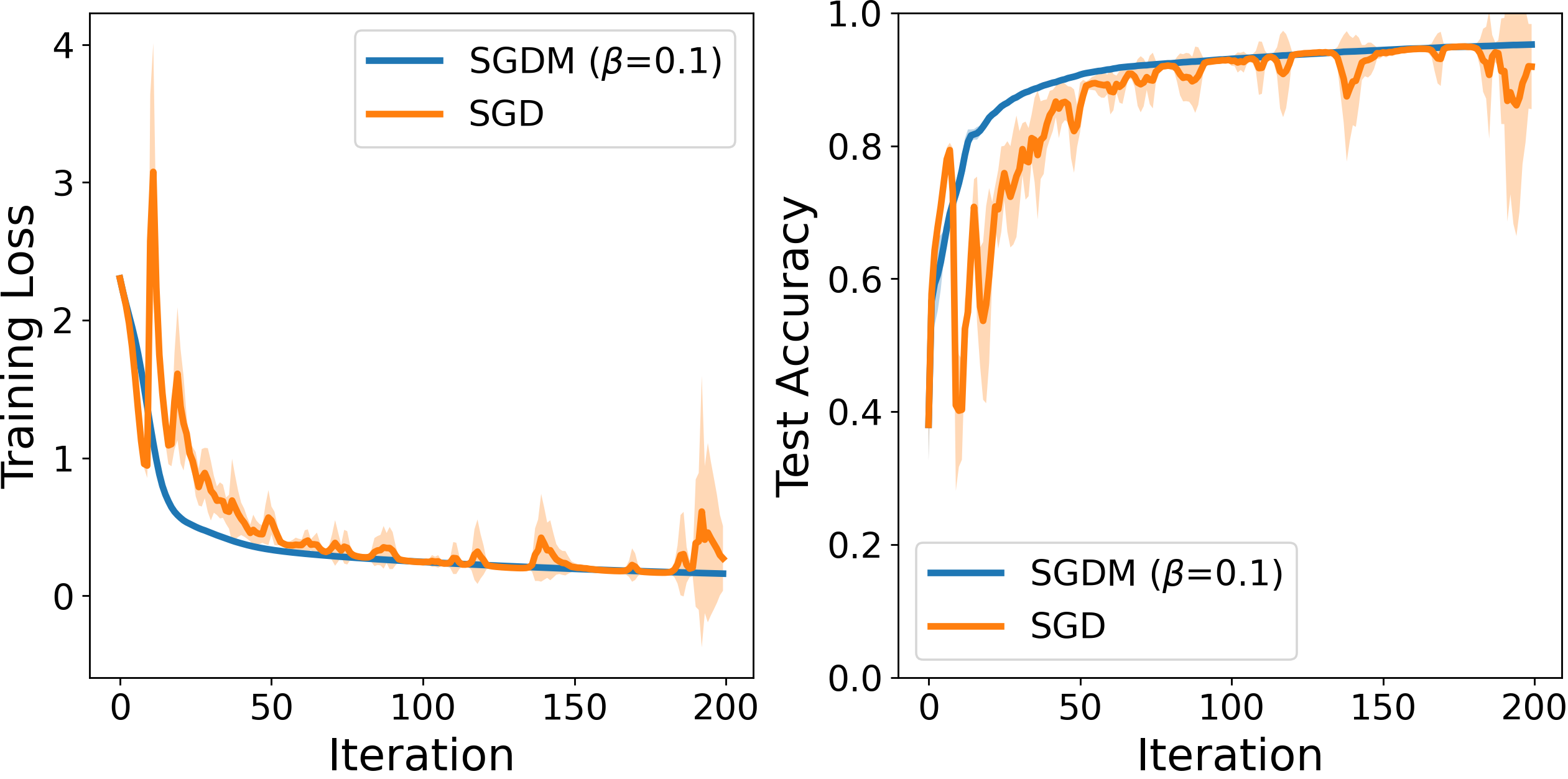
(a) Top-2% sparsification

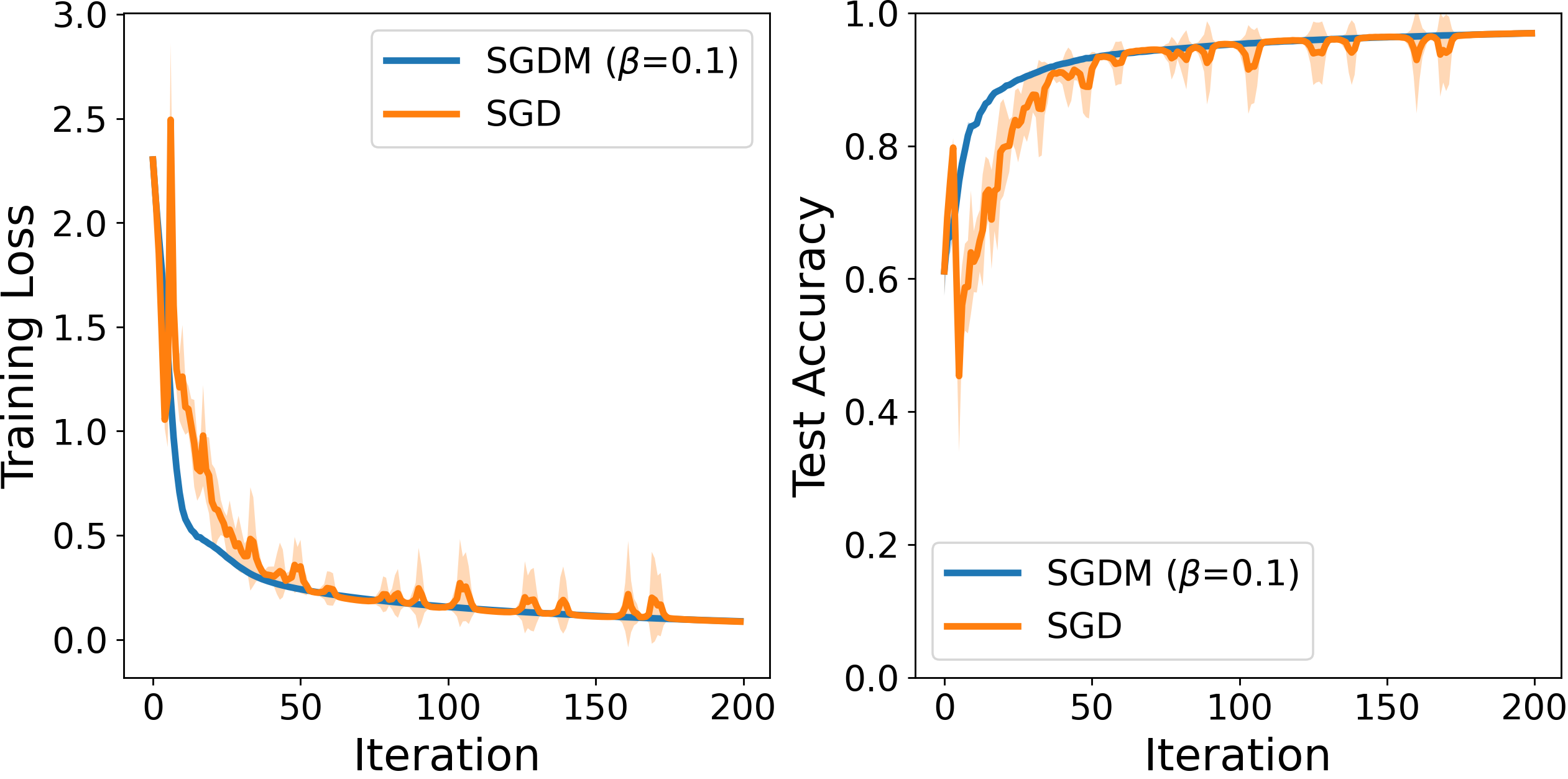
(b) Clipped with $\tau=2$

(c) Top-0.1% sparsification

(d) Clipped with $\tau=2$

Figure 1: Performance of distributed SGDM (i.e., momentum method) and SGD method under various biased gradient estimations ((a) and (c) compressed gradients; (b) and (d) clipped gradients) in terms of (left plots -) training loss and (right plots -) test accuracy on (top plots -) MNIST and (bottom plots -) FashionMNIST datasets, considering $n=100$ and $\gamma=0.5$.

VI Proofs

VI-A Proof of Lemma 1

Let $\gamma^{k}=\gamma$ and $\beta^{k}=\beta$. We prove the result in two steps.

Step 1) The upper bounds for $\|\nabla f(x^{k})-v^{k}\|^{2}$ and $\|\nabla f(x^{k+1})-v^{k}\|^{2}$

First, we bound $\|\nabla f(x^{k})-v^{k}\|^{2}$. By the convexity of the squared norm, for $0\leq\beta\leq 1$,

$$\|\nabla f(x^{k})-v^{k}\|^{2}\leq(1-\beta)\|\nabla f(x^{k})-v^{k-1}\|^{2}+\beta\|\eta^{k}\|^{2},$$ (19)

where $\eta^{k}=(1/n)\sum_{i=1}^{n}\tilde{\nabla}f_{i}(x^{k})-\nabla f(x^{k})$. Second, we bound $\|\nabla f(x^{k+1})-v^{k}\|^{2}$ as follows:

$$\|\nabla f(x^{k+1})-v^{k}\|^{2}\mathop{\leq}^{\eqref{eqn:theta_x_y}+\eqref{eqn:descent_interm_x_v}}(1+\theta)(1-\beta)\|\nabla f(x^{k})-v^{k-1}\|^{2}$$

$$\hskip 14.22636pt+(1+\theta)\beta\|\eta^{k}\|^{2}+(1+1/\theta)\|\nabla f(x^{k+1})-\nabla f(x^{k})\|^{2}.$$

If $\theta=\beta/2$, then by the fact that $(1+\beta/2)(1-\beta)\leq 1-\beta/2$ and by Assumption 1

$$\|\nabla f(x^{k+1})-v^{k}\|^{2}\leq(1-\beta/2)\|\nabla f(x^{k})-v^{k-1}\|^{2}$$

$$\hskip 14.22636pt+(1+\beta/2)\beta\|\eta^{k}\|^{2}+(1+2/\beta)L^{2}\|x^{k+1}-x^{k}\|^{2}.$$ (20)

Step 2) The descent inequality

Define $\phi^{k}:=f(x^{k})-f^{\star}+A\|\nabla f(x^{k})-v^{k-1}\|^{2}$ with $A>0$. If $\gamma\leq 1/L$, then

$$\phi^{k+1} \mathop{\leq}^{\eqref{eqn:smoothness_ineq}}f(x^{k})-f^{\star}-\frac{\gamma}{2}\|\nabla f(x^{k})\|^{2}-D_{1}\|x^{k+1}-x^{k}\|^{2}$$

$$\hskip 14.22636pt+\frac{\gamma}{2}\|\nabla f(x^{k})-v^{k}\|^{2}+A\|\nabla f(x^{k+1})-v^{k}\|^{2}.$$

where $D_{1}=\frac{1}{2\gamma}-\frac{L}{2}$. Next, plugging (19) and (20) into the main inequality yields

$$\phi^{k+1} \leq f(x^{k})-f^{\star}-\frac{\gamma}{2}\|\nabla f(x^{k})\|^{2}+B_{1}\|\nabla f(x^{k})-v^{k-1}\|^{2}$$

$$\hskip 14.22636pt-B_{2}\|x^{k+1}-x^{k}\|^{2}+B_{3}\|\eta^{k}\|^{2},$$

where $B_{1}=\gamma(1-\beta)/2+A(1-\beta/2)$, $B_{2}=\frac{1}{2\gamma}-\frac{L}{2}-A\frac{(\beta+2)L^{2}}{\beta}$, and $B_{3}=\gamma\beta/2+A\beta(1+\beta/2)$.

VI-B Proof of Theorem 1

VI-B1 Proof of Theorem 1-1

If $A=\frac{\gamma}{\beta}(1-\beta)$, then from (9)

$$\phi^{k+1} \leq\phi^{k}-\frac{\gamma}{2}\|\nabla f(x^{k})\|^{2}-\Theta\|x^{k+1}-x^{k}\|^{2}$$

$$\hskip 14.22636pt+\gamma(1-\beta^{2}/2)\|\eta^{k}\|^{2},$$

where $\Theta=\frac{1}{2\gamma}-\frac{L}{2}-{\gamma}\cdot\frac{(1-\beta)(\beta+2)L^{2}}{\beta^{2}}$. From Lemma 3 with $a=1/2$, $b=L/2$ and $c=\frac{(1-\beta)(\beta+2)L^{2}}{\beta^{2}}$, we can prove that if $0<\gamma\leq\frac{1}{L}\cdot\frac{1}{\sqrt{\frac{2(1-\beta)(\beta+2)}{\beta^{2}}}+1}$, then $\Theta\geq 0$ and thus

$$\phi^{k+1} \leq\phi^{k}-\frac{\gamma}{2}\|\nabla f(x^{k})\|^{2}+\gamma(1-\beta^{2}/2)\|\eta^{k}\|^{2}.$$

Next, by taking the expectation and using the fact that $\mathbf{E}\|\eta^{k}\|^{2}\leq B\mathbf{E}\|\nabla f(x^{k})\|^{2}+C$ for $B,C\geq 0$,

$$\mathbf{E}[\phi^{k+1}] \leq\mathbf{E}[\phi^{k}]-\gamma D\mathbf{E}\|\nabla f(x^{k})\|^{2}+\gamma(1-\beta^{2}/2)C,$$

where $D=1/2-(1-\beta^{2}/2)B$.

If $(1-\beta^{2}/2)B\leq 1/4$, then $D\geq 1/4$ and

$$\mathbf{E}[\phi^{k+1}] \leq\mathbf{E}[\phi^{k}]-\frac{\gamma}{4}\mathbf{E}\|\nabla f(x^{k})\|^{2}+\gamma(1-\beta^{2}/2)C.$$

Therefore, by the fact that $\min_{0\leq k\leq K-1}\mathbf{E}\|\nabla f(x^{k})\|^{2}\leq\frac{1}{K}\sum_{k=0}^{K-1}\mathbf{E}\|\nabla f(x^{k})\|^{2}$, by the main inequality above, and by the consequence of telescopic series,

$$\min_{0\leq k\leq K-1}\mathbf{E}\|\nabla f(x^{k})\|^{2} \leq\frac{4}{\gamma}\frac{\mathbf{E}[\phi^{0}]}{K}+4(1-\beta^{2}/2)C.$$

Finally, by the definition of $\phi^{0}$, we complete the proof.

VI-B2 Proof of Theorem 1-2

If $A=\frac{2\gamma}{\beta}(1-\beta)$, then from (9)

$$\phi^{k+1}\leq f(x^{k})-f^{\star}-\frac{\gamma}{2}\|\nabla f(x^{k})\|^{2}$$

$$+A(1-\beta/4)\|\nabla f(x^{k})-v^{k-1}\|^{2}-\hat{\Theta}\|x^{k+1}-x^{k}\|^{2}$$

$$+\gamma(2-\beta/2-\beta^{2})\|\eta^{k}\|^{2},$$

where $\hat{\Theta}=\frac{1}{2\gamma}-\frac{L}{2}-\gamma\frac{2(1-\beta)(\beta+2)L^{2}}{\beta^{2}}$.

From Lemma 3 with $a=1/2$, $b=L/2$ and $c=\frac{2(1-\beta)(\beta+2)L^{2}}{\beta^{2}}$, we can prove that if $0<\gamma\leq\frac{1}{\sqrt{\frac{4(1-\beta)(\beta+2)L^{2}}{\beta^{2}}}+L}$, then $\hat{\Theta}\geq 0$ and thus

$$\phi^{k+1}\leq f(x^{k})-f^{\star}-\frac{\gamma}{2}\|\nabla f(x^{k})\|^{2}$$

$$+A(1-\beta/4)\|\nabla f(x^{k})-v^{k-1}\|^{2}+\gamma(2-\beta/2-\beta^{2})\|\eta^{k}\|^{2}.$$

Next, by taking the expectation and using the fact that $\mathbf{E}\|\eta^{k}\|^{2}\leq B\mathbf{E}\|\nabla f(x^{k})\|^{2}+C$ for $B,C\geq 0$,

$$\mathbf{E}[\phi^{k+1}]\leq\mathbf{E}[f(x^{k})-f^{\star}]-\gamma\Theta_{1}\mathbf{E}\|\nabla f(x^{k})\|^{2}$$

$$+A(1-\beta/4)\mathbf{E}\|\nabla f(x^{k})-v^{k-1}\|^{2}+\gamma(2-\beta/2-\beta^{2})C,$$

where $\Theta_{1}=1/2-(2-\beta/2-\beta^{2})B$.

If $(2-\beta/2-\beta^{2})B\leq 1/4$, then by Assumption 2

$$\mathbf{E}[\phi^{k+1}]\leq(1-\mu\gamma/2)\mathbf{E}[f(x^{k})-f^{\star}]$$

$$+A(1-\beta/4)\mathbf{E}\|\nabla f(x^{k})-v^{k-1}\|^{2}+\gamma(2-\beta/2-\beta^{2})C.$$

If $\gamma\leq\frac{\beta}{2\mu}$, then

$$\mathbf{E}[\phi^{k+1}] \leq(1-\mu\gamma/2)\mathbf{E}[\phi^{k}]+\gamma(2-\beta/2-\beta^{2})C.$$

Finally, applying this inequality over $k=0,1,\ldots,K-1$ yields

$$\mathbf{E}[\phi^{K}] \leq(1-\mu\gamma/2)^{K}\phi^{0}+\frac{2}{\mu}(2-\beta/2-\beta^{2})C.$$

VI-C Proof of Proposition 1

The compressed momentum methods (10) are momentum methods in Eq. (7) and (8) where $\eta^{k}=\frac{1}{n}\sum_{i=1}^{n}Q(g_{i}^{k})-\nabla f(x^{k})$. From Lemma 4 with $G(g_{i}^{k})=Q(g_{i}^{k})$, and by (12)

$$\|\eta^{k}\|^{2}\leq\frac{B_{1}}{n}\sum_{i=1}^{n}\|g_{i}^{k}\|^{2}+\frac{B_{2}}{n}\sum_{i=1}^{n}\|g_{i}^{k}-\nabla f_{i}(x^{k})\|^{2},$$

where $B_{1}=(1+\theta_{1})(1-\alpha)$ and $B_{2}=(1+1/\theta_{1})$.

If $\theta_{1}=\alpha/2$, then $(1+\theta_{1})(1-\alpha)\leq 1-\alpha/2$ and by (23) with $x=\nabla f_{i}(x^{k})$ and $y=g_{i}^{k}-\nabla f_{i}(x^{k})$,

$$\|\eta^{k}\|^{2}\leq\frac{\hat{B}_{1}}{n}\sum_{i=1}^{n}\|\nabla f_{i}(x^{k})\|^{2}+\frac{\hat{B}_{2}}{n}\sum_{i=1}^{n}\|g_{i}^{k}-\nabla f_{i}(x^{k})\|^{2},$$

where $\hat{B}_{1}=(1+\theta_{2})(1-\alpha/2)$ and $\hat{B}_{2}=(1+1/\theta_{2})(1-\alpha/2)+(1+2/\alpha)$.

If $\theta_{2}=\alpha/4$, then $(1+\theta_{2})(1-\alpha/2)\leq 1-\alpha/4$ and by (23) with $x=\nabla f(x^{k})$ and $y=\nabla f_{i}(x^{k})-\nabla f(x^{k})$

$$\|\eta^{k}\|^{2}\leq \bar{B}_{1}\|\nabla f(x^{k})\|^{2}+\frac{\bar{B}_{2}}{n}\sum_{i=1}^{n}\|\nabla f_{i}(x^{k})-\nabla f(x^{k})\|^{2}$$

$$+\frac{\bar{B}_{3}}{n}\sum_{i=1}^{n}\|g_{i}^{k}-\nabla f_{i}(x^{k})\|^{2},$$

where $\bar{B}_{1}=(1+\theta_{3})(1-\alpha/4)$, $\bar{B}_{2}=(1+1/\theta_{3})(1-\alpha/4)$ and $\bar{B}_{3}=(1+4/\alpha)(1-\alpha/2)+(1+2/\alpha)$. Finally, If $\theta_{3}=\alpha/8$, then $(1+\theta_{3})(1-\alpha/4)\leq 1-\alpha/8$, and then by taking the expectation and by using the fact that $\mathbf{E}\|g_{i}^{k}-\nabla f_{i}(x^{k})\|^{2}\leq\sigma^{2}$ and that $\|\nabla f_{i}(x)-\nabla f(x)\|^{2}\leq\delta^{2}$ for $x\in\mathbb{R}^{d}$, we complete the proof.

VI-D Proof of Proposition 2

We first introduce one useful lemma for proving the result.

Lemma 2.

For any $\tau>0$ and $g\in\mathbb{R}^{d}$, $\|\mathbf{clip}_{\tau}(g)-g\|\leq\max(\|g\|-\tau,0)$.

Proof.

From the definition of the clipping operator and the Euclidean norm,

$$\|\mathbf{clip}_{\tau}(g)-g\| =(\|g\|-\tau)\cdot\mathbbm{1}(\|g\|>\tau)+0\cdot\mathbbm{1}(\|g\|\leq\tau)$$

$$\leq\max(\|g\|-\tau,0).$$

∎

Now, we prove the result. The compressed momentum methods (10) are momentum methods in Eq. (7) and (8) where $\eta^{k}=\frac{1}{n}\sum_{i=1}^{n}\mathbf{clip}_{\tau}(g_{k}^{i})-\nabla f(x^{k})$. From Lemma 4 with $G(g_{i}^{k})=\mathbf{clip}_{\tau}(g_{k}^{i})$ and $\theta=2$,

$$\|\eta^{k}\|^{2}\leq\frac{2}{n}\sum_{i=1}^{n}\|\mathbf{clip}_{\tau}(g_{k}^{i})-g_{i}^{k}\|^{2}+\frac{2}{n}\sum_{i=1}^{n}\|g_{i}^{k}-\nabla f_{i}(x^{k})\|^{2}.$$

By the fact that $\|g_{i}^{k}-\nabla f_{i}(x^{k})\|^{2}\leq\sigma^{2}$,

$$\|\eta^{k}\|^{2}\leq\frac{2}{n}\sum_{i=1}^{n}\|\mathbf{clip}_{\tau}(g_{k}^{i})-g_{i}^{k}\|^{2}+2\sigma^{2}.$$

To complete the proof, we bound $\|\mathbf{clip}_{\tau}(g_{k}^{i})-g_{i}^{k}\|^{2}$. By Lemma 2, and the fact that $\tau>0$ and that $\|x\|\geq 0$ for $x\in\mathbb{R}^{d}$,

$$\frac{1}{n}\sum_{i=1}^{n}\|\mathbf{clip}_{\tau}(g_{k}^{i})-g_{i}^{k}\|^{2} \leq\max\left(\frac{1}{n}\sum_{i=1}^{n}[\|g_{i}^{k}\|-\tau]^{2},0\right)$$

$$\leq\max\left(\frac{1}{n}\sum_{i=1}^{n}\|g_{i}^{k}\|^{2}+\tau^{2},0\right).$$

Since, by (23) with $\theta=2$, and by the fact that $f_{i}(x)$ has $L$-Lipschitz continuous gradient, that $\|g_{i}^{k}-\nabla f_{i}(x^{k})\|^{2}\leq\sigma^{2}$ and that $f(x^{k})-f(x^{\star})\leq\delta$,

$$\frac{1}{n}\sum_{i=1}^{n}\|g_{i}^{k}\|^{2} \leq\frac{2}{n}\sum_{i=1}^{n}\|g_{i}^{k}-\nabla f_{i}(x^{k})\|^{2}+\frac{2}{n}\sum_{i=1}^{n}\|\nabla f_{i}(x^{k})\|^{2}$$

$$\leq 2\sigma^{2}+4L[f(x^{k})-f(x^{\star})]\leq 2\sigma^{2}+4L\delta,$$

we have

$$\frac{1}{n}\sum_{i=1}^{n}\|\mathbf{clip}_{\tau}(g_{k}^{i})-g_{i}^{k}\|^{2} \leq\max(2\sigma^{2}+4L\delta+\tau^{2},0).$$

Therefore,

$$\|\eta^{k}\|^{2}\leq 2\max(2\sigma^{2}+4L\delta+\tau^{2},0)+2\sigma^{2}.$$

Finally taking the expectation, we complete the proof.

VI-E Proof of Proposition 3

If each $g_{i,j}(x)$ is $\ell_{g}$-Lipschitz continuous and has $L_{g}$-Lipschitz continuous gradient, then by Cauchy-Schwartz’s inequality $g_{i}(x)=\frac{1}{m_{g}}\sum_{j=1}^{m_{g}}g_{i,j}(x)$ is also $\ell_{g}$-Lipschitz continuous and has $L_{g}$-Lipschitz continuous gradient. Similarly, if each $F_{i,j}(x)$ is $\ell_{F}$-Lipschitz continuous and has $L_{F}$-Lipschitz continuous gradient, then by Cauchy-Schwartz’s inequality $F_{i}(x)=\frac{1}{m_{F}}\sum_{j=1}^{m_{F}}F_{i,j}(x)$ is also $\ell_{F}$-Lipschitz continuous and has $L_{F}$-Lipschitz continuous gradient.

VI-E1 Proof of Proposition 3-1

We next prove the first statement. By the triangle inequality and by the fact that $\nabla f(x)=\frac{1}{n}\sum_{i=1}^{n}\nabla f_{i}(x)$ and $\nabla f_{i}(x)=\langle g^{\prime}_{i}(x),F^{\prime}_{i}(g_{i}(x))\rangle$,

$$\|\nabla f(x)-\nabla f(y)\| \leq\frac{1}{n}\sum_{i=1}^{n}\|\nabla f_{i}(x)-\nabla f_{i}(y)\|$$

$$=\frac{1}{n}\sum_{i=1}^{n}\|T_{1}+T_{2}\|\leq\frac{1}{n}\sum_{i=1}^{n}\left(\bar{T}_{1}+\bar{T}_{2}\right),$$

where $T_{1}=\langle g^{\prime}_{i}(x),F^{\prime}_{i}(g_{i}(x))\rangle-\langle g^{\prime}_{i}(y),F^{\prime}_{i}(g_{i}(x))\rangle$, $T_{2}=\langle g^{\prime}_{i}(y),F^{\prime}_{i}(g_{i}(x))\rangle-\langle g^{\prime}_{i}(y),F^{\prime}_{i}(g_{i}(y))\rangle$, $\bar{T}_{1}=\|F^{\prime}_{i}(g_{i}(x))\|\cdot\|g^{\prime}_{i}(x)-g^{\prime}_{i}(y)\|$, and $\bar{T}_{2}=\|g^{\prime}_{i}(y)\|\cdot\|F^{\prime}_{i}(g_{i}(x))-F^{\prime}_{i}(g_{i}(y))\|$. Next, by the $L_{g}$-Lipschitz continuity of $g_{i}^{\prime}(x)$ and the $\ell_{F}$-Lipschitz continuity of $F_{i}(x)$, we have $T_{1}\leq L_{g}\ell_{F}\|x-y\|$, and

$$\|\nabla f(x)-\nabla f(y)\| \leq\frac{1}{n}\sum_{i=1}^{n}\left(L_{g}\ell_{F}\|x-y\|+\bar{T}_{2}\right),$$

Next, by the $\ell_{g}$-Lipschitz continuity of $g_{i}(x)$ and the $L_{F}$-Lipschitz continuity of $F_{i}^{\prime}(x)$, we have

$$T_{2} \leq\ell_{g}L_{F}\|g_{i}(x)-g_{i}(y)\|\leq\ell_{g}^{2}L_{F}\|x-y\|.$$

Therefore,

$$\|\nabla f(x)-\nabla f(y)\|\leq(L_{g}\ell_{F}+\ell_{g}^{2}L_{F})\|x-y\|.$$

VI-E2 Proof of Proposition 3-2

We finally prove the second statement.

Let $\bar{v}^{k}:=\frac{1}{|\mathcal{S}_{g}^{k}|}\sum_{j\in\mathcal{S}_{g}^{k}}g_{i,j}(x^{k})$ and $\bar{z}^{k}:=\frac{1}{|\mathcal{S}_{g}^{k}|}\sum_{j\in\mathcal{S}_{g}^{k}}g_{i,j}^{\prime}(x^{k})$. From the definition of the Euclidean norm, and by the fact that $\eta^{k}=\frac{1}{n}\sum_{i=1}^{n}\tilde{\nabla}f_{i}(x^{k})-\nabla f_{i}(x^{k})$,

$$\|\eta^{k}\|^{2} \mathop{\leq}\limits^{\eqref{eqn:Jensen}}\frac{1}{n}\sum_{i=1}^{n}\|\tilde{\nabla}f_{i}(x^{k})-\nabla f_{i}(x^{k})\|^{2},$$

where $\tilde{\nabla}f_{i}(x^{k})=\left\langle\bar{z}^{k},\frac{1}{|\mathcal{S}_{F}^{k}|}\sum_{j\in\mathcal{S}_{F}^{k}}F_{i,j}^{\prime}\left(\bar{v}^{k}\right)\right\rangle$ and $\nabla f_{i}(x^{k})=\left\langle g^{\prime}_{i}(x^{k}),F_{i}^{\prime}\left(g_{i}(x^{k})\right)\right\rangle$. Next, by the fact that $\|x+y+z\|^{2}\leq 3\|x\|^{2}+3\|y\|^{2}+3\|z\|^{2}$ with $x=\left\langle\bar{z}^{k},\frac{1}{|\mathcal{S}_{F}^{k}|}\sum_{j\in\mathcal{S}_{F}^{k}}F_{i,j}^{\prime}\left(\bar{v}^{k}\right)\right\rangle-\left\langle\bar{z}^{k},F_{i}^{\prime}(\bar{v}^{k})\right\rangle$, $y=\left\langle\bar{z}^{k},F_{i}^{\prime}(\bar{v}^{k})\right\rangle-\left\langle g^{\prime}_{i}(x^{k}),F_{i}^{\prime}(\bar{v}^{k})\right\rangle$, and $z=\left\langle g^{\prime}_{i}(x^{k}),F_{i}^{\prime}(\bar{v}^{k})\right\rangle-\left\langle g^{\prime}_{i}(x^{k}),F_{i}^{\prime}\left(g_{i}(x^{k})\right)\right\rangle$,

$$\|\eta^{k}\|^{2} \leq 3\|\bar{z}^{k}\|^{2}\left\|\frac{1}{|\mathcal{S}_{F}^{k}|}\sum_{j\in\mathcal{S}_{F}^{k}}F_{i,j}^{\prime}\left(\bar{v}^{k}\right)-F_{i}^{\prime}(\bar{v}^{k})\right\|^{2}$$

$$+3\|F_{i}^{\prime}(\bar{v}^{k})\|^{2}\left\|\bar{z}^{k}-g^{\prime}_{i}(x^{k})\right\|^{2}$$

$$+3\|g_{i}^{\prime}(x^{k})\|^{2}\left\|F_{i}^{\prime}(\bar{v}^{k})-F_{i}^{\prime}\left(g_{i}(x^{k})\right)\right\|^{2}.$$

Since each $g_{i,j}(x)$ is $\ell_{g}$-Lipschitz continuous and each $F_{i,j}(x)$ is $\ell_{F}$-Lipschitz continuous, by (24) we have

$$\|\bar{z}^{k}\|^{2} \leq\frac{1}{|\mathcal{S}_{g}^{k}|}\sum_{j\in\mathcal{S}_{g}^{k}}\|g_{i,j}^{\prime}(x^{k})\|^{2}\leq\ell_{g}^{2},$$

$$\|g^{\prime}(x^{k})\|^{2} \leq\frac{1}{m_{g}}\sum_{j=1}^{m_{g}}\|g^{\prime}_{i,j}(x^{k})\|^{2}\leq\ell_{g}^{2},\quad\text{and}$$

$$\|F_{i}^{\prime}\left(v^{k}\right)\|^{2} \leq\frac{1}{m_{F}}\sum_{j=1}^{m_{F}}\|F^{\prime}_{i,j}(v^{k})\|^{2}\leq\ell_{F}^{2}.$$

Therefore, plugging these results into the main inequality,

$$\|\eta^{k}\|^{2} \leq 3\ell_{g}^{2}\left\|\frac{1}{|\mathcal{S}_{F}^{k}|}\sum_{j\in\mathcal{S}_{F}^{k}}F_{i,j}^{\prime}\left(\bar{v}^{k}\right)-F_{i}^{\prime}(\bar{v}^{k})\right\|^{2}$$

$$+3\ell_{F}^{2}\left\|\bar{z}^{k}-g^{\prime}_{i}(x^{k})\right\|^{2}$$

$$+3\ell_{g}^{2}\left\|F_{i}^{\prime}(\bar{v}^{k})-F_{i}^{\prime}\left(g_{i}(x^{k})\right)\right\|^{2}.$$

Since each $F_{i,j}(x)$ has $L_{F}$-Lipschitz continuous gradient, $F_{i}(x)$ has also $L_{F}$-Lipschitz continuous gradient. Hence, using this fact and taking the expectation,

$$\mathbf{E}\|\eta^{k}\|^{2} \leq 3\ell_{g}^{2}\mathbf{E}\left\|\frac{1}{|\mathcal{S}_{F}^{k}|}\sum_{j\in\mathcal{S}_{F}^{k}}F_{i,j}^{\prime}\left(\bar{v}^{k}\right)-F_{i}^{\prime}(\bar{v}^{k})\right\|^{2}$$

$$+3\ell_{F}^{2}\mathbf{E}\left\|\bar{z}^{k}-g^{\prime}_{i}(x^{k})\right\|^{2}$$

$$+3\ell_{g}^{2}L_{F}^{2}\mathbf{E}\left\|\bar{v}^{k}-g_{i}(x^{k})\right\|^{2}.$$

Assuming that $\mathcal{S}_{g}^{k}$ and $\mathcal{S}_{F}^{k}$ are sampled uniformly at random, we get $\mathbf{E}\left[\frac{1}{|\mathcal{S}_{g}^{k}|}\sum_{j\in\mathcal{S}_{g}^{k}}g_{i,j}(x^{k})\right]=g_{i}(x^{k})$, $\mathbf{E}\left[\frac{1}{|\mathcal{S}_{g}^{k}|}\sum_{j\in\mathcal{S}_{g}^{k}}g^{\prime}_{i,j}(x^{k})\right]=g^{\prime}_{i}(x^{k})$ and $\mathbf{E}\left[\frac{1}{|\mathcal{S}_{F}^{k}|}\sum_{j\in\mathcal{S}_{F}^{k}}F_{i,j}^{\prime}\left(\bar{v}^{k}\right)\right]=F^{\prime}_{i}(\bar{v}^{k})$. In addition,

$$\mathbf{E}\left\|\frac{1}{|\mathcal{S}_{F}^{k}|}\sum_{j\in\mathcal{S}_{F}^{k}}F_{i,j}^{\prime}\left(\bar{v}^{k}\right)-F_{i}^{\prime}(\bar{v}^{k})\right\|^{2} \leq\frac{\sigma_{F}^{2}}{|\mathcal{S}_{F}^{k}|},$$

$$\mathbf{E}\left\|\bar{z}^{k}-g^{\prime}_{i}(x^{k})\right\|^{2} \leq\frac{\sigma_{g^{\prime}}^{2}}{|\mathcal{S}_{g}^{k}|},\quad\text{and}$$

$$\mathbf{E}\left\|\bar{v}^{k}-g_{i}(x^{k})\right\|^{2} \leq\frac{\sigma_{g}^{2}}{|\mathcal{S}_{g}^{k}|}.$$

Therefore,

$$\mathbf{E}\|\eta^{k}\|^{2}\leq 3\ell_{g}^{2}\frac{\sigma_{F}^{2}}{|\mathcal{S}_{F}^{k}|}+3\ell_{F}^{2}\frac{\sigma_{g^{\prime}}^{2}}{|\mathcal{S}_{g}^{k}|}+3\ell_{g}^{2}L_{F}^{2}\frac{\sigma_{g}^{2}}{|\mathcal{S}_{g}^{k}|}.$$

Finally, setting $|\mathcal{S}_{F}^{k}|=S_{F}$ and $|\mathcal{S}_{g}^{k}|=S_{g}$ yields the result.

VI-F Proof of Proposition 4

Let $\ell_{i}(x,a^{j}_{i},b^{j}_{i})$ be $\ell_{l}$-Lipschitz continuous and have $L_{l}$-Lipschitz continuous gradient. By the fact that $F_{i,j}(x)=\ell_{i}(x,a^{j}_{i},b^{j}_{i})$,

$$\|F_{i,j}(x)-F_{i,j}(y)\| =\|\ell_{i}(x,a^{j}_{i},b^{j}_{i})-\ell_{i}(y,a^{j}_{i},b^{j}_{i})\|$$

$$\leq\ell_{l}\|x-y\|,\quad\text{and}$$

$$\|F^{\prime}_{i,j}(x)-F^{\prime}_{i,j}(y)\| =\|\nabla\ell_{i}(x,a^{j}_{i},b^{j}_{i})-\nabla\ell_{i}(y,a^{j}_{i},b^{j}_{i})\|$$

$$\leq L_{l}\|x-y\|.$$

Next, by the fact that $g_{i,j}(x)=x-\gamma\nabla\ell_{i}(x,a^{j}_{i},b^{j}_{i})$,

$$\|g_{i,j}(x)-g_{i,j}(y)\| \leq\|x-y\|+\gamma T_{1}\leq(1+\gamma L_{l})\|x-y\|,$$

where $T_{1}=\|\nabla\ell_{i}(x,a^{j}_{i},b^{j}_{i})-\nabla\ell_{i}(y,a^{j}_{i},b^{j}_{i})\|$. In addition, we can show that $g^{\prime}_{i,j}(x)=I-\gamma\nabla^{2}\ell_{i}(x,a^{j}_{i},b^{j}_{i})$, and that

$$\|g^{\prime}_{i,j}(x)-g^{\prime}_{i,j}(y)\| \leq\gamma\|\nabla^{2}\ell_{i}(x,a^{j}_{i},b^{j}_{i})-\nabla^{2}\ell_{i}(y,a^{j}_{i},b^{j}_{i})\|$$

$$\leq\gamma(B(x)+B(y))\leq 2\gamma L_{l},$$

where $B(x)=\|\nabla^{2}\ell_{i}(x,a^{j}_{i},b^{j}_{i})\|$.

VII Conclusion

We unify a convergence analysis framework for distributed stochastic momentum methods with biased gradients. We show that biased momentum methods attain the convergence bound similar to biased SGD for general non-convex and $\mu$-PL non-convex problems. Based on our results, we also establish convergence for distributed momentum methods with compressed, clipped, and composite gradients, including distributed MAML. Numerical experiments validated stronger convergence performance of biased momentum methods than biased gradient descent in convergence speed and solution accuracy. As future work, establishing convergence results based on our analysis framework in other applications, including reinforcement learning and risk-aware learning, would be considered a worthwhile study.

Appendix A Basic Facts

We use the following facts from linear algebra: for any $x,y\in\mathbb{R}^{d}$ and $\theta>0$,

$$2\langle x,y\rangle =\|x\|^{2}+|y\|^{2}-\|x-y\|^{2}.$$ (21)

$$2\langle x,y\rangle \leq\theta\|x\|^{2}+\theta^{-1}\|y\|^{2}.$$ (22)

$$\|x+y\|^{2} \leq(1+\theta)\|x\|^{2}+(1+\theta^{-1})\|y\|^{2}.$$ (23)

For vectors $x_{1},x_{2},\ldots,x_{N}\in\mathbb{R}^{d}$, Jensen’s inequality and the convexity of the squared norm yields

$$\left\|\frac{1}{N}\sum_{i=1}^{N}x_{i}\right\|^{2}\leq\frac{1}{N}\sum_{i=1}^{N}\|x_{i}\|^{2}.$$ (24)

The next lemma allows us to obtain the upper bound for the step-size satisfying the specific inequality.

Lemma 3 (Lemma 5 of [61]).

Let $a,b,c>0$. If $0<\gamma\leq(\sqrt{\nicefrac{{c}}{{a}}}+\nicefrac{{b}}{{a}})^{-1}$, then $\frac{a}{\gamma}-b-c\gamma\geq 0$.

Furthermore, we introduce the next lemma, which is useful for deriving the upper bound for $\|\eta^{k}\|^{2}$ in Section IV.

Lemma 4.

Let $f(x)=(1/n)\sum_{i=1}^{n}f_{i}(x)$ and $\eta=(1/n)\sum_{i=1}^{n}G(g_{i}^{k})-\nabla f(x^{k})$ for any operator $G:\mathbb{R}^{d}\rightarrow\mathbb{R}^{d}$. Then, for $\theta>0$,

$$\|\eta^{k}\|^{2}\leq(1+\theta)T_{1}^{k}+(1+1/\theta)T_{2}^{k},$$ (25)

where $T_{1}^{k}=\frac{1}{n}\sum_{i=1}^{n}\|G(g_{i}^{k})-g_{i}^{k}\|^{2}$ and $T_{2}^{k}=\frac{1}{n}\sum_{i=1}^{n}\|g_{i}^{k}-\nabla f_{i}(x^{k})\|^{2}$.

Proof.

By the fact that $\nabla f(x)=(1/n)\sum_{i=1}^{n}\nabla f_{i}(x)$, and from the definition of the Euclidean norm and $\eta^{k}$, we have $\|\eta^{k}\|^{2}=\left\|({1}/{n})\sum_{i=1}^{n}[G(g_{i}^{k})-\nabla f_{i}(x^{k})]\right\|^{2}.$ Finally, by (24) and then by (23), we complete the proof. ∎

Appendix B Additional Numerical Evaluations on Deep Neural Networks

Additional learning curves are included in this section. To be more specific, Figure 2 contains learning curves for the MNIST dataset using FCNN. Also, more results for both the MNIST dataset and the FashionMNIST dataset are included in the following link: https://github.com/AliBeikmohammadi/DistributedSGDM/ (See Figures 3-9), utilizing FCNN and ResNet-18 model, respectively. Again, the shaded regions correspond to the standard deviation of the average evaluation over five trials.

(a) Top-5% sparsification

(b) Clipped with $\tau=1$

(c) Top-10% sparsification

(d) Clipped with $\tau=5$

Figure 2: Results on MNIST dataset, considering $n=100$ and $\gamma=0.5$ - FCNN.

References

- [1] Q. V. Le, J. Ngiam, A. Coates, A. Lahiri, B. Prochnow, and A. Y. Ng, “On optimization methods for deep learning,” in Proceedings of the 28th International Conference on International Conference on Machine Learning, 2011, pp. 265–272.
- [2] A. Coates, A. Ng, and H. Lee, “An analysis of single-layer networks in unsupervised feature learning,” in Proceedings of the fourteenth international conference on artificial intelligence and statistics. JMLR Workshop and Conference Proceedings, 2011, pp. 215–223.
- [3] M. Li, L. Zhou, Z. Yang, A. Li, F. Xia, D. G. Andersen, and A. Smola, “Parameter server for distributed machine learning,” in Big learning NIPS workshop, vol. 6, no. 2, 2013.
- [4] A. Krizhevsky, I. Sutskever, and G. E. Hinton, “Imagenet classification with deep convolutional neural networks,” Communications of the ACM, vol. 60, no. 6, pp. 84–90, 2017.
- [5] I. Sutskever, J. Martens, G. Dahl, and G. Hinton, “On the importance of initialization and momentum in deep learning,” in International conference on machine learning. PMLR, 2013, pp. 1139–1147.
- [6] L. Bottou, “Stochastic gradient descent tricks,” Neural Networks: Tricks of the Trade: Second Edition, pp. 421–436, 2012.
- [7] ——, “Large-scale machine learning with stochastic gradient descent,” in Proceedings of COMPSTAT’2010: 19th International Conference on Computational StatisticsParis France, August 22-27, 2010 Keynote, Invited and Contributed Papers. Springer, 2010, pp. 177–186.
- [8] M. Zinkevich, M. Weimer, L. Li, and A. Smola, “Parallelized stochastic gradient descent,” Advances in neural information processing systems, vol. 23, 2010.
- [9] I. Loshchilov and F. Hutter, “SGDR: Stochastic gradient descent with warm restarts,” arXiv preprint arXiv:1608.03983, 2016.
- [10] H. R. Feyzmahdavian, A. Aytekin, and M. Johansson, “An asynchronous mini-batch algorithm for regularized stochastic optimization,” IEEE Transactions on Automatic Control, vol. 61, no. 12, pp. 3740–3754, 2016.
- [11] S. Khirirat, H. R. Feyzmahdavian, and M. Johansson, “Mini-batch gradient descent: Faster convergence under data sparsity,” in 2017 IEEE 56th Annual Conference on Decision and Control (CDC). IEEE, 2017, pp. 2880–2887.
- [12] R. Ge, S. M. Kakade, R. Kidambi, and P. Netrapalli, “The step decay schedule: A near optimal, geometrically decaying learning rate procedure for least squares,” Advances in neural information processing systems, vol. 32, 2019.
- [13] X. Wang, S. Magnússon, and M. Johansson, “On the convergence of step decay step-size for stochastic optimization,” Advances in Neural Information Processing Systems, vol. 34, pp. 14 226–14 238, 2021.
- [14] O. Sebbouh, R. M. Gower, and A. Defazio, “Almost sure convergence rates for stochastic gradient descent and stochastic heavy ball,” in Conference on Learning Theory. PMLR, 2021, pp. 3935–3971.
- [15] B. E. Woodworth, K. K. Patel, and N. Srebro, “Minibatch vs local SGD for heterogeneous distributed learning,” Advances in Neural Information Processing Systems, vol. 33, pp. 6281–6292, 2020.
- [16] D. Csiba and P. Richtárik, “Importance sampling for minibatches,” The Journal of Machine Learning Research, vol. 19, no. 1, pp. 962–982, 2018.
- [17] L. Xiao and T. Zhang, “A proximal stochastic gradient method with progressive variance reduction,” SIAM Journal on Optimization, vol. 24, no. 4, pp. 2057–2075, 2014.
- [18] R. Johnson and T. Zhang, “Accelerating stochastic gradient descent using predictive variance reduction,” Advances in neural information processing systems, vol. 26, 2013.
- [19] K. Mishchenko, A. Khaled, and P. Richtárik, “Random reshuffling: Simple analysis with vast improvements,” Advances in Neural Information Processing Systems, vol. 33, pp. 17 309–17 320, 2020.
- [20] J. Haochen and S. Sra, “Random shuffling beats SGD after finite epochs,” in International Conference on Machine Learning. PMLR, 2019, pp. 2624–2633.
- [21] M. Gürbüzbalaban, A. Ozdaglar, and P. A. Parrilo, “Why random reshuffling beats stochastic gradient descent,” Mathematical Programming, vol. 186, pp. 49–84, 2021.
- [22] D. Alistarh, D. Grubic, J. Li, R. Tomioka, and M. Vojnovic, “QSGD: communication-efficient SGD via gradient quantization and encoding,” Advances in neural information processing systems, vol. 30, 2017.
- [23] S. Khirirat, H. R. Feyzmahdavian, and M. Johansson, “Distributed learning with compressed gradients,” arXiv preprint arXiv:1806.06573, 2018.
- [24] S. Khirirat, M. Johansson, and D. Alistarh, “Gradient compression for communication-limited convex optimization,” in 2018 IEEE Conference on Decision and Control (CDC). IEEE, 2018, pp. 166–171.
- [25] A. Beznosikov, S. Horváth, P. Richtárik, and M. Safaryan, “On biased compression for distributed learning,” arXiv preprint arXiv:2002.12410, 2020.
- [26] R. Pascanu, T. Mikolov, and Y. Bengio, “On the difficulty of training recurrent neural networks,” in International conference on machine learning. Pmlr, 2013, pp. 1310–1318.
- [27] D. Alistarh, Z. Allen-Zhu, and J. Li, “Byzantine stochastic gradient descent,” Advances in Neural Information Processing Systems, vol. 31, 2018.
- [28] K. Pillutla, S. M. Kakade, and Z. Harchaoui, “Robust aggregation for federated learning,” IEEE Transactions on Signal Processing, vol. 70, pp. 1142–1154, 2022.
- [29] L. Li, W. Xu, T. Chen, G. B. Giannakis, and Q. Ling, “RSA: byzantine-robust stochastic aggregation methods for distributed learning from heterogeneous datasets,” in Proceedings of the AAAI Conference on Artificial Intelligence, vol. 33, no. 01, 2019, pp. 1544–1551.
- [30] C. Finn, P. Abbeel, and S. Levine, “Model-agnostic meta-learning for fast adaptation of deep networks,” in International conference on machine learning. PMLR, 2017, pp. 1126–1135.
- [31] A. Ruszczynski and W. Syski, “Stochastic approximation method with gradient averaging for unconstrained problems,” IEEE Transactions on Automatic Control, vol. 28, no. 12, pp. 1097–1105, 1983.
- [32] A. Ajalloeian and S. U. Stich, “On the convergence of SGD with biased gradients,” arXiv preprint arXiv:2008.00051, 2020.
- [33] Y. Liu, Y. Gao, and W. Yin, “An improved analysis of stochastic gradient descent with momentum,” Advances in Neural Information Processing Systems, vol. 33, pp. 18 261–18 271, 2020.
- [34] D. Needell, R. Ward, and N. Srebro, “Stochastic gradient descent, weighted sampling, and the randomized kaczmarz algorithm,” Advances in neural information processing systems, vol. 27, 2014.
- [35] D. P. Bertsekas et al., “Incremental gradient, subgradient, and proximal methods for convex optimization: A survey,” Optimization for Machine Learning, vol. 2010, no. 1-38, p. 3, 2011.
- [36] B. T. Polyak, “Some methods of speeding up the convergence of iteration methods,” Ussr computational mathematics and mathematical physics, vol. 4, no. 5, pp. 1–17, 1964.
- [37] Y. E. Nesterov, “A method of solving a convex programming problem with convergence rate ,” in Doklady Akademii Nauk, vol. 269, no. 3. Russian Academy of Sciences, 1983, pp. 543–547.
- [38] A. Gupal and L. Bazhenov, “Stochastic analog of the conjugant-gradient method,” Cybernetics, vol. 8, no. 1, pp. 138–140, 1972.
- [39] Y. Yan, T. Yang, Z. Li, Q. Lin, and Y. Yang, “A unified analysis of stochastic momentum methods for deep learning,” arXiv preprint arXiv:1808.10396, 2018.
- [40] H. Yu, R. Jin, and S. Yang, “On the linear speedup analysis of communication efficient momentum SGD for distributed non-convex optimization,” in International Conference on Machine Learning. PMLR, 2019, pp. 7184–7193.
- [41] J. Ma and D. Yarats, “Quasi-hyperbolic momentum and adam for deep learning,” arXiv preprint arXiv:1810.06801, 2018.
- [42] H. Wang, Y. Luo, W. An, Q. Sun, J. Xu, and L. Zhang, “Pid controller-based stochastic optimization acceleration for deep neural networks,” IEEE transactions on neural networks and learning systems, vol. 31, no. 12, pp. 5079–5091, 2020.
- [43] E. Ghadimi, H. R. Feyzmahdavian, and M. Johansson, “Global convergence of the heavy-ball method for convex optimization,” in 2015 European control conference (ECC). IEEE, 2015, pp. 310–315.
- [44] N. Loizou and P. Richtárik, “Linearly convergent stochastic heavy ball method for minimizing generalization error,” arXiv preprint arXiv:1710.10737, 2017.
- [45] M. Assran and M. Rabbat, “On the convergence of nesterov’s accelerated gradient method in stochastic settings,” arXiv preprint arXiv:2002.12414, 2020.
- [46] R. Xin and U. A. Khan, “Distributed heavy-ball: A generalization and acceleration of first-order methods with gradient tracking,” IEEE Transactions on Automatic Control, vol. 65, no. 6, pp. 2627–2633, 2019.
- [47] G. Garrigos and R. M. Gower, “Handbook of convergence theorems for (stochastic) gradient methods,” arXiv preprint arXiv:2301.11235, 2023.
- [48] T. H. Tran, L. M. Nguyen, and Q. Tran-Dinh, “SMG: a shuffling gradient-based method with momentum,” in International Conference on Machine Learning. PMLR, 2021, pp. 10 379–10 389.
- [49] S. P. Karimireddy, Q. Rebjock, S. Stich, and M. Jaggi, “Error feedback fixes signsgd and other gradient compression schemes,” in International Conference on Machine Learning. PMLR, 2019, pp. 3252–3261.
- [50] J. Zhang, T. He, S. Sra, and A. Jadbabaie, “Why gradient clipping accelerates training: A theoretical justification for adaptivity,” arXiv preprint arXiv:1905.11881, 2019.
- [51] V. V. Mai and M. Johansson, “Stability and convergence of stochastic gradient clipping: Beyond lipschitz continuity and smoothness,” in International Conference on Machine Learning. PMLR, 2021, pp. 7325–7335.
- [52] B. Zhang, J. Jin, C. Fang, and L. Wang, “Improved analysis of clipping algorithms for non-convex optimization,” Advances in Neural Information Processing Systems, vol. 33, pp. 15 511–15 521, 2020.
- [53] D. P. Bertsekas and J. N. Tsitsiklis, “Gradient convergence in gradient methods with errors,” SIAM Journal on Optimization, vol. 10, no. 3, pp. 627–642, 2000.
- [54] H. Karimi, J. Nutini, and M. Schmidt, “Linear convergence of gradient and proximal-gradient methods under the polyak-łojasiewicz condition,” in Machine Learning and Knowledge Discovery in Databases: European Conference, ECML PKDD 2016, Riva del Garda, Italy, September 19-23, 2016, Proceedings, Part I 16. Springer, 2016, pp. 795–811.
- [55] D. J. Foster, A. Sekhari, and K. Sridharan, “Uniform convergence of gradients for non-convex learning and optimization,” Advances in Neural Information Processing Systems, vol. 31, 2018.
- [56] Y. Lei, T. Hu, G. Li, and K. Tang, “Stochastic gradient descent for nonconvex learning without bounded gradient assumptions,” IEEE transactions on neural networks and learning systems, vol. 31, no. 10, pp. 4394–4400, 2019.
- [57] C. Herrera, F. Krach, and J. Teichmann, “Estimating full lipschitz constants of deep neural networks,” arXiv preprint arXiv:2004.13135, 2020.
- [58] M. Faw, I. Tziotis, C. Caramanis, A. Mokhtari, S. Shakkottai, and R. Ward, “The power of adaptivity in SGD: Self-tuning step sizes with unbounded gradients and affine variance,” in Conference on Learning Theory. PMLR, 2022, pp. 313–355.
- [59] F. Khani and P. Liang, “Feature noise induces loss discrepancy across groups,” in International Conference on Machine Learning. PMLR, 2020, pp. 5209–5219.
- [60] H. Xu, C. Caramanis, and S. Mannor, “Robust regression and lasso,” Advances in neural information processing systems, vol. 21, 2008.
- [61] P. Richtárik, I. Sokolov, and I. Fatkhullin, “EF21: a new, simpler, theoretically better, and practically faster error feedback,” Advances in Neural Information Processing Systems, vol. 34, pp. 4384–4396, 2021.
- [62] S. Khirirat, S. Magnússon, A. Aytekin, and M. Johansson, “A flexible framework for communication-efficient machine learning,” in Proceedings of the AAAI Conference on Artificial Intelligence, vol. 35, no. 9, 2021, pp. 8101–8109.
- [63] J. Zhang, S. P. Karimireddy, A. Veit, S. Kim, S. Reddi, S. Kumar, and S. Sra, “Why are adaptive methods good for attention models?” Advances in Neural Information Processing Systems, vol. 33, pp. 15 383–15 393, 2020.
- [64] Z. Huo, B. Gu, J. Liu, and H. Huang, “Accelerated method for stochastic composition optimization with nonsmooth regularization,” in Proceedings of the AAAI Conference on Artificial Intelligence, vol. 32, no. 1, 2018.
- [65] A. Shapiro, D. Dentcheva, and A. Ruszczynski, Lectures on stochastic programming: modeling and theory. SIAM, 2021.
- [66] P. Ravikumar, J. Lafferty, H. Liu, and L. Wasserman, “Sparse additive models,” Journal of the Royal Statistical Society: Series B (Statistical Methodology), vol. 71, no. 5, pp. 1009–1030, 2009.
- [67] A. Fallah, A. Mokhtari, and A. Ozdaglar, “Personalized federated learning with theoretical guarantees: A model-agnostic meta-learning approach,” Advances in Neural Information Processing Systems, vol. 33, pp. 3557–3568, 2020.
- [68] M. Wang, E. X. Fang, and H. Liu, “Stochastic compositional gradient descent: algorithms for minimizing compositions of expected-value functions,” Mathematical Programming, vol. 161, pp. 419–449, 2017.
- [69] Y. LeCun, “The mnist database of handwritten digits,” http://yann. lecun. com/exdb/mnist/, 1998.
- [70] H. Xiao, K. Rasul, and R. Vollgraf, “Fashion-mnist: a novel image dataset for benchmarking machine learning algorithms,” arXiv preprint arXiv:1708.07747, 2017.
- [71] K. He, X. Zhang, S. Ren, and J. Sun, “Deep residual learning for image recognition,” in Proceedings of the IEEE conference on computer vision and pattern recognition, 2016, pp. 770–778.