Quantum Bayesian Inference with Renormalization for Gravitational Waves

Abstract

Advancements in gravitational-wave interferometers, particularly the next generation, are poised to profoundly impact gravitational wave astronomy and multimessenger astrophysics. A hybrid quantum algorithm is proposed to carry out quantum inference of parameters from compact binary coalescences detected in gravitational-wave interferometers. It performs quantum Bayesian Inference with Renormalization and Downsampling (qBIRD). We choose binary black hole (BBH) mergers from LIGO observatories as the first case to test the algorithm, but its application can be extended to more general instances. The quantum algorithm is able to generate corner plots of relevant parameters such as chirp mass, mass ratio, spins, etc. by inference of simulated gravitational waves with known injected parameter values with zero noise, Gaussian noise and real data, thus recovering an accuracy equivalent to that of classical Markov Chain Monte Carlo inferences. The simulations are performed with sets of 2 and 4 parameters. These results enhance the possibilities to extend our capacity to track signals from coalescences over longer durations and at lower frequencies extending the accuracy and promptness of gravitational wave parameter estimation.

Introduction.— The Advanced LIGO and Advanced Virgo observatories have detected a large volume of gravitational waves (GWs) from compact binary coalescences [1, 2, 3] since their first observation of a BBH merger in 2015 [4]. A network of third-generation (3G) gravitational wave (GW) observatories, such as Cosmic Explorer (CE) [5], Einstein Telescope (ET) [6], and Neutron Star Extreme Matter Observatory (NEMO) [7] will significantly advance our capacity in detecting GW, including those from compact binary coalescences, core-collapse supernovae, and rotating compact objects [8]. Consequently, GW inference will face unprecedented challenges [9]. Moreover, in an era of thousands of detections per day, the majority of the signals are overlapped. With the sensitivity improvements in low frequency band, signals can be tracked at lower frequencies and over much longer durations, extending from currently seconds to hours. These challenges cannot be addressed by traditional parameter estimation tools.

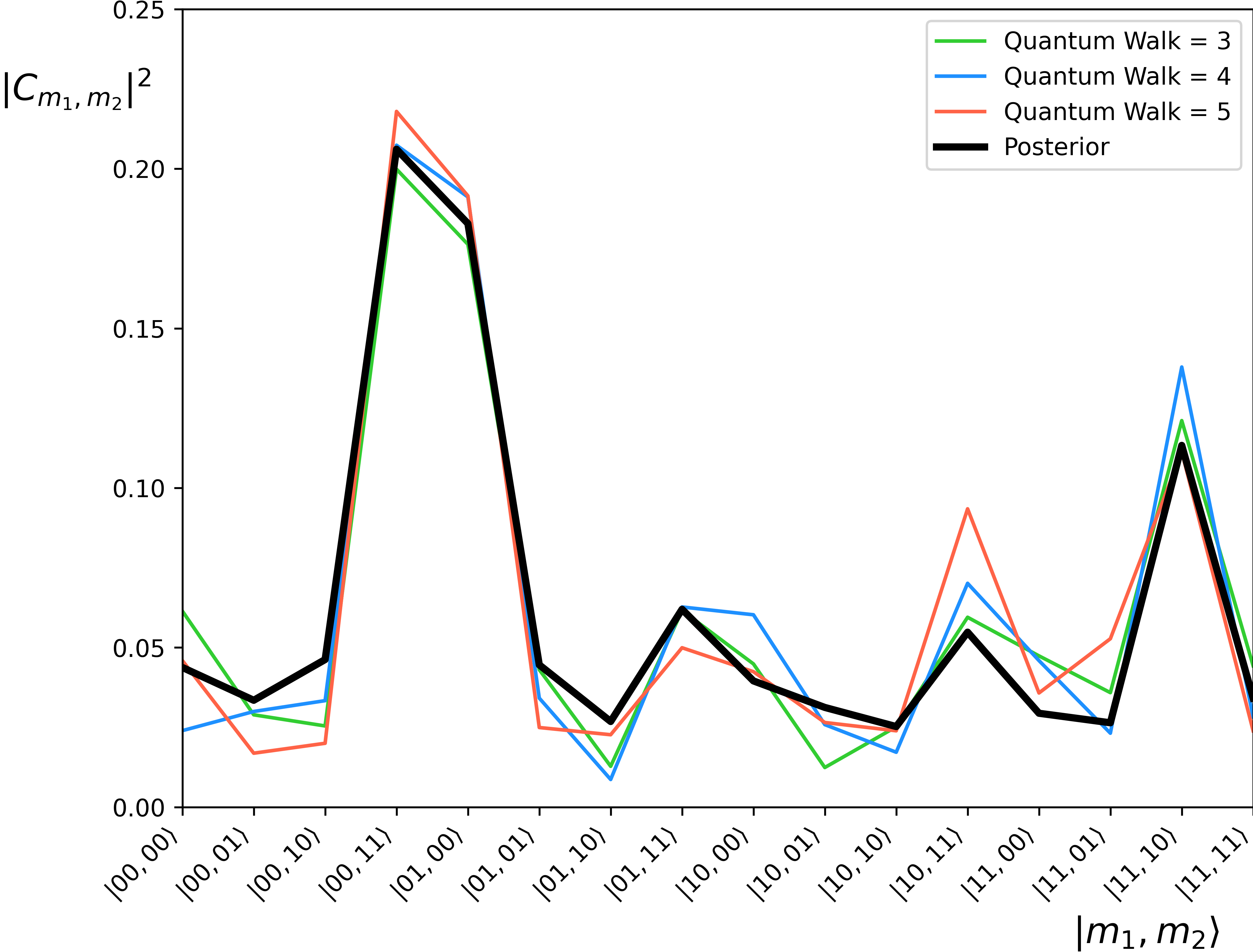
Quantum computing arises as a promising candidate for accurate and accelerated GW inference. Quantum techniques are particularly useful for search and sampling problems [10], as shown in Fig. 1. In our previous study [11], we proved a polynomial scaling quantum advantage over classical algorithms in ranking GW likelihoods. In this work, we develop a comprehensive computational framework that implements a quantum version of the classical Markov Chain Monte Carlo (MCMC) technique [12], specifically, its archetype, the Metropolis-Hastings (MH) algorithm [13] to compute posterior probability density functions (PDFs) of GW source parameters, achieving accuracy comparable to classical methods [14, 15]. In this work, we introduce qBIRD, a quantum algorithm for GW source characterization using Bayesian inference with renormalization and downsampling. We showcase the sampler’s accuracy by inferring synthetic and observed GW signals from merging BBHs.

GW likelihood.—For a detected gravitational wave, Bayesian inference is applied to characterize source properties. Given data $d$ and model $M$, characterizing the parameter space $\bm{\theta}$ that models a gravitational wave signal $h(\bm{\theta})$ is estimating the posterior probabilities $p(\bm{\theta}|d,M)$. Bayes’ theorem yields these posteriors as

$$\small p(\bm{\theta}|d,M)=\frac{\pi(\bm{\theta}|M){\cal L}(d|\bm{\theta},M)}{Z_{M}},$$ (1)

where $\pi(\bm{\theta}|M)$ is the prior probability that models the belief in $\bm{\theta}$ under $M$, ${\cal L}(d|\bm{\theta},M)$ is the gravitational wave likelihood representing the probability of observed data $d$ given the parameters $\bm{\theta}$ and model $M$. $Z_{M}=\int{\cal L}(d|\bm{\theta},M)\pi(\bm{\theta}|M)d\bm{\theta}$ is the normalization constant for the marginalized posterior likelihood, or evidence. The inference process involves computing and ranking the likelihoods between gravitational wave signals $h(\bm{\theta})$ predicted by theory and the noisy observed data $d$. Since the noise in observed GW data is typically Gaussian, the standard GW likelihood follows a Gaussian about the square root of the power spectral density (PSD), $S_{n}$, namely,

$$\small{\cal L}(d|\text{\boldmath{\hbox{\theta}}},M)\propto\text{exp}\left(-\sum_{i=1}^{T}\frac{2|{d}(f_{i})-{h}(f_{i};\text{\boldmath{\hbox{\theta}}})|^{2}}{TS_{n}(f_{i})}\right),$$ (2)

where $T$ is the total number of frequency nodes.

The GW posterior in Eqn. (1) has two important properties for our purposes of constructing a hybrid quantum algorithm for parameter estimation based on renormalization methods (see Step 1 later): i) the GW likelihood only depends on the noise (S.I.3) and is the product of the individual frequency bins likelihoods; ii) the source property priors are independent:

$$\small\pi(\text{\boldmath{\hbox{\theta}}}|M)=\prod_{p=1}^{P}\pi(\theta_{p}|M),$$ (3)

with $P$ the total number of parameters inferred, reflecting the fact that the intrinsic parameters are uncorrelated one another. Similarly, for the extrinsic parameters. These factorization properties are the base for the truncation (renormalization) in the quantum space of states representing all parameters that lead to the formulation of our algorithm that is presented and employed below.

Figure 1: Colour lines represent the state register probabilities $\ket{\bm{\theta}}_{S}=\ket{m_{1},m_{2}}_{S}$ for different number of applications of the quantum walk operator in Eqn. (5). It is a two source masses inference, using $Q=2$ discretization qubits, for the event GW150914. X-axis is composed by the 16 combinations that represents the binary encoding of a value for the first mass and another value for the second mass. The black line represents the posterior probability function in Eqn. (1) of each of these combinations.

Quantum Metropolis algorithm.—Parameter estimation from GW data involves stochastic sampling techniques to draw samples from the posterior distribution in Eqn. (1). In GW community, this statistical analysis primarily relies on MCMC methods [16], demanding computationally intensive numerical methods and high-performance computers. This opens the door to applying quantum algorithms of the form developed in this work. Several approaches have been proposed to extend the classical Metropolis algorithms to the quantum domain [17], showing an expected quantum advantage over its classical counterpart [18, 19]. In this work, we introduce a hybrid Metropolis heuristic algorithm based on quantum walks called qBIRD, quantum Bayesian Inference with Renormalization and Downsampling. This approach allows us to obtain results from injections or real data [20, 21], that not only showcase the quantum computational advantages but also demonstrate comparable performance to classical methods [15, 14].

A quantum walk can be viewed as an agent that explores the parameter space in superposition [22], which is endowed with a quantum Hilbert space [23] of states specified as follows. Let $\Theta$ be the configuration space of the parameters $\theta$ we want to infer from the experimental data. The dimensionality of this space depends on the total number of parameters, about 20 for a typical binary merger event. $\Theta$ must be discretized with a certain grid or lattice that also depends on the precision used to represent each parameter $\theta_{p}$. Our choice is a hypercube lattice with periodic boundary conditions that allow quantum walks between nearest-neighbor vertices.

To specify a quantum walk in this space state of parameters, we use 3 quantum registers, similar to other quantum walk proposals [19, 24]. First, a register of states $\ket{\text{\boldmath$\theta$}}_{S}$ stores the information of the parameter values. A second register $\ket{p}_{D}$ encodes the hopping directions of the walker in binary notation corresponding to the oriented edges of the lattice. A third register $\ket{\Delta\text{\boldmath$\theta$}}_{E}$ stores the information of, given parameter $\theta_{p}$, moves to a neighbor site by shiftting the parameter an amount $\Delta\theta_{p}$ or an amount $-\Delta\theta_{p}$. Additionally, a coin state $\ket{\varphi}_{C}$ accounts for the random evolution of the walker. Finally, an auxiliary register $\ket{A(\bm{\theta},\bm{\theta}+\Delta\bm{\theta})}_{A}$ stores the acceptance probabilities of each transition. These are given by the MH acceptance rule:

$$\small A(\bm{\theta},\bm{\theta}+\Delta\bm{\theta})=\min[1,\frac{\pi(\bm{\theta}+\Delta\bm{\theta})}{\pi(\bm{\theta})}(\frac{\mathcal{L}(d|\bm{\theta}+\Delta\bm{\theta})}{\mathcal{L}(d|\bm{\theta})})^{\beta}],$$ (4)

where $\beta$ represents an annealing schedule.

The quantum walk employs a total of $PQ+\lceil\log_{2}P\rceil+a+2$ qubits: $PQ$ represents the number of qubits needed for register $\ket{\text{\boldmath$\theta$}}_{S}$ that contains all the points of the lattice $\Theta$, where $P$ is the number of inferred parameters and $Q$ is the number of discretization qubits, with $2^{Q}$ states represented for each parameter; $\lceil\log_{2}P\rceil$ qubits to represent register $\ket{p}_{D}$ in binary encoding; $a$ qubits to represent the auxiliary register for the acceptance probability. Finally, 2 qubits are needed, one for the register $\ket{\Delta\text{\boldmath$\theta$}}_{E}$, and another for the coin register $\ket{\varphi}_{C}$ to encode the accept/reject probability of all states.

Figure 2: Flowchart of qBIRD algorithm. See main text for module and step explanations.

Now, the evolution operator $W$ of the quantum walk is constructed over the previous registers as follows (see S.II for its detailed construction):

$$W=RV^{\dagger}B^{\dagger}SFBV.$$ (5)

This allows us to construct the one-step circuit of the quantum walk, with $W$ as a building block of a quantum MH algorithm. By applying several $W$ consecutively, a quantum walk traverses the parameter space $\Theta$ according to certain transition probabilities, just as the classical MH does. The operator $W$ skillfully samples the posterior distribution in Eqn. (1), storing it as state probabilities, as seen in Fig. 1. This shows that the crucial aspect underpinning the superiority of the quantum algorithm over its classical counterpart lies in the fact that each measurement simulates the probability of accepting each state, capitalizing on the efficiency of superposition. Prior research demonstrated that the results of the quantum MH algorithm is achieved with a polynomial scaling advantage over its classical counterpart [11].

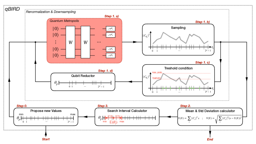
qBIRD algorithm.—Using the above quantum walk as a core, we have developed a hybrid algorithm capable of inferring the posterior probability-density functions of the source parameters from gravitational wave radiation obtained from binary BHs merger events, and can be used for any type of GW source. qBIRD consists of three modules: the quantum Metropolis module, the renormalization and downsampling module and a classical postprocessing module. The description of the algorithm is as follows, and is illustrated schematically in Fig. 2.

Step 0. Parameter initialization: The algorithm is initialized by proposing $2^{Q}$ values for each parameter, drawn from a uniform distribution specified by the lower and upper bounds of the prior function (3). All these values are stored in the state register $\ket{\text{\boldmath$\theta$}}_{S}$ producing an initial state $\ket{\phi^{(0)}}$.

Step 1. Renormalization & Downsampling: This first module executes the quantum metropolis algorithm of (5) and is adapted from [25] and endowed with a renormalization method that defines the qBIRD algorithm. In this step, the quantum walk will be applied several times as we decrease the parameter space $\Theta$ to locate the set of values for each parameter $\theta_{p}$ maximizing the likelihood.

a) Quantum Metropolis: Iteratively apply the walk operator (5) $L$ times on the initial state, which contains $|S|:=s=PQ$ qubits:

$$\ket{\psi(L)}:=W_{L}...W_{2}W_{1}\ket{\phi^{(0)}}.$$ (6)

The integer $s$ is also used as the index of the renormalization module step.

b) Sampling: Sample the state register $\ket{\text{\boldmath$\theta$}}_{S}$

$$\small\ket{\bm{\theta}}_{S}:=\sum_{x\in\Theta(s)}C_{x}\ket{x}_{S},$$ (7)

from $\ket{\text{\boldmath$\theta$}}_{S}$ measurements to obtain the pairs $\{|C_{x}|^{2},x\}_{s}$. $\Theta(s)$ denotes the state space of qubits at the $s$-th step of the renormalization procedure to be described in d).

c) Threshold condition: If $s=P$, jump to Step 2, otherwise calculate the number of elements $|S_{h}(s)|$ with:

$$\small S_{h}(s):=\left\{y\in\Theta(s):|C_{y}|^{2}\geq\alpha\underset{x\in\Theta(s)}{\max}|C_{x}|^{2}\right\},$$ (8)

where $\alpha\in[0,1]$ represents a threshold and $S_{h}(s)$ is a sieve to obtain it.

d) Qubit reductor: Reduce the number of qubits in the state register $\ket{\text{\boldmath$\theta$}}_{S}$ by defining

$$\small s^{\prime}:=\max\left[P,\min\left(\lceil\log_{2}|S_{h}(s)|\rceil,s-P\right)\right],$$ (9)

and go to Step 1a) with $s^{\prime}$ qubits and the $2^{s^{\prime}}$ highest probability values. This condition allows us to eliminate at least one qubit for each parameter, ending up with a minimum of one qubit per parameter.

This second module arises from the challenge of using the quantum metropolis algorithm to search for the state with the maximum probability and is inspired by the renormalization techniques of quantum lattice models [26]. Due to the enormous size of the state space, the normalization factor of quantum states results in very small probability differences between the most and least probable states. Although the probability disparity between states may span a couple of orders of magnitude, obtaining significance would require an impractical number of measurements. During the discretization process, the evidence in (1) is proportional to the size of the lattice, $Z_{M}\propto|\Theta|$. Then, as we increase the size of the parameter space $\Theta$, the closer to zero the probabilities will be. It is important to note that this problem is specific to Bayes’ theorem and has not been introduced by using quantum computing. However, if we gradually remove the states that are significantly less probable by reducing the size and qubits of the problem, these differences become progressively more noticeable. With this technique, we are able to find the state with the maximum likelihood over all the proposed values.

The effectiveness of the quantum renormalization method in computing the maximum likelihood shown in Eqn. (1) lies in the well-suited truncations in Hilbert space of states for uncorrelated noise (Gaussian) describing the likelihood (2) and the BH parameters (3), as exemplified by properties i) and ii) after Eqn. (2).

Figure 3: Posterior distributions obtained with qBIRD for the chirp mass $\mathcal{M}_{c}$ and mass ratio $q$ of a simulated BBH gravitational wave signal injected into Gaussian-noise using PyCBC. The injected values are $\mathcal{M}_{c}=19.50\ {\text{M}_{\odot}}$ and $q=2.00$, shown in orange.

Step 2. Mean & Std Deviation calculator: The third module consists of a classical processing that takes the results obtained in the first two modules to generate PDFs for each parameter and converge the algorithm. Thus, given the pairs, $\{|C_{x}|^{2},x\}_{s=P}$ compute:

$$\mathbb{E}(\theta_{p}) :=\sum_{x\in\theta_{p}(s=P)}|C_{x}|^{2}x,$$ (10)

$$V(\theta_{p}) :=\sqrt{\sum_{x\in\theta_{p}(s=P)}|C_{x}|^{2}(x-\mathbb{E}(\theta_{p}))^{2}},$$ (11)

which represent the mean and weighted standard deviation for each parameter $p=1,\dotsb,P$, respectively. It is important to save the $\mathbb{E}(\theta_{p})$ values in each iteration in order to build the PDFs at the end of the algorithm.

Step 3. Search interval calculator: To gradually narrow down the search area, a new interval for each parameter is proposed from $\mathbb{E}(\theta_{p})$ and $V(\theta_{p})$ previously obtained, with lower and upper values given by:

$$\theta_{p,(\text{min},\text{max})}=\mathbb{E}(\theta_{p})\mp\lambda V(\theta_{p}),$$ (12)

where $\lambda$ is a parameter to be set for controlling the convergence of the algorithm. Note that the proposed new minimum (maximum) cannot be lower (greater) than the one set by prior interval (3). Then return to Step 0 with the new interval $[\mathbb{E}(\theta_{p})-\lambda V(\theta_{p}),\mathbb{E}(\theta_{p})+\lambda V(\theta_{p})]$.

End. After a given number of iterations of Steps $0-3$, PDFs of each of the parameters $\theta_{p}$ are constructed from the $\mathbb{E}(\theta_{p})$ values obtained in each iteration. Then corner plots visualize the PDFs of the inference.

Figure 4: Posterior distributions obtained with qBIRD for a synthetic BBH signal characterized with 4 unknown parameters. The simulated gravitational wave was injected into zero-noise using Bilby, and the injected values are $\mathcal{M}_{c}=27.43\ {\text{M}_{\odot}}$, $q=0.57$, $d_{L}=2000\text{ Mpc}$, and $\theta_{jn}=0.70$, shown in orange.

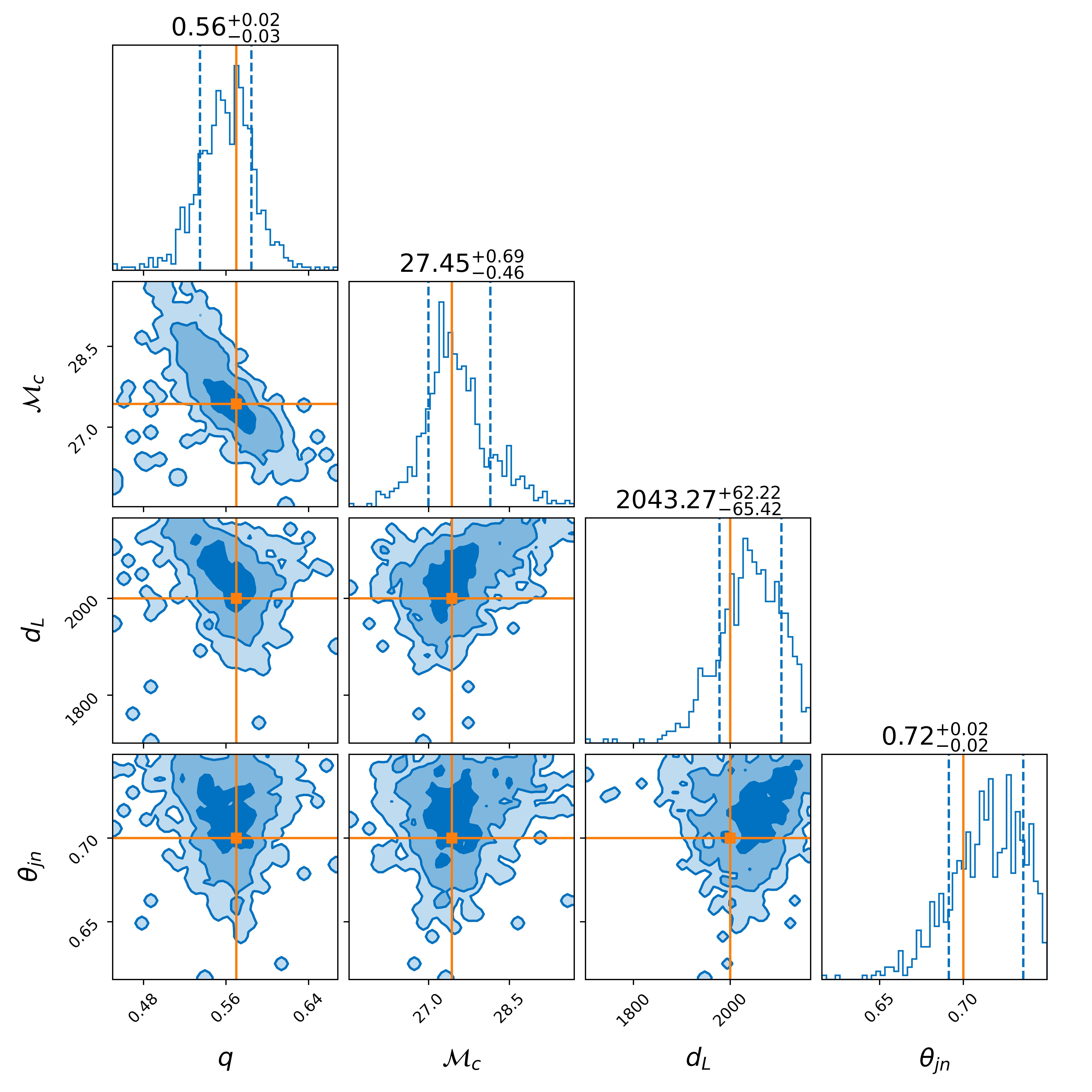
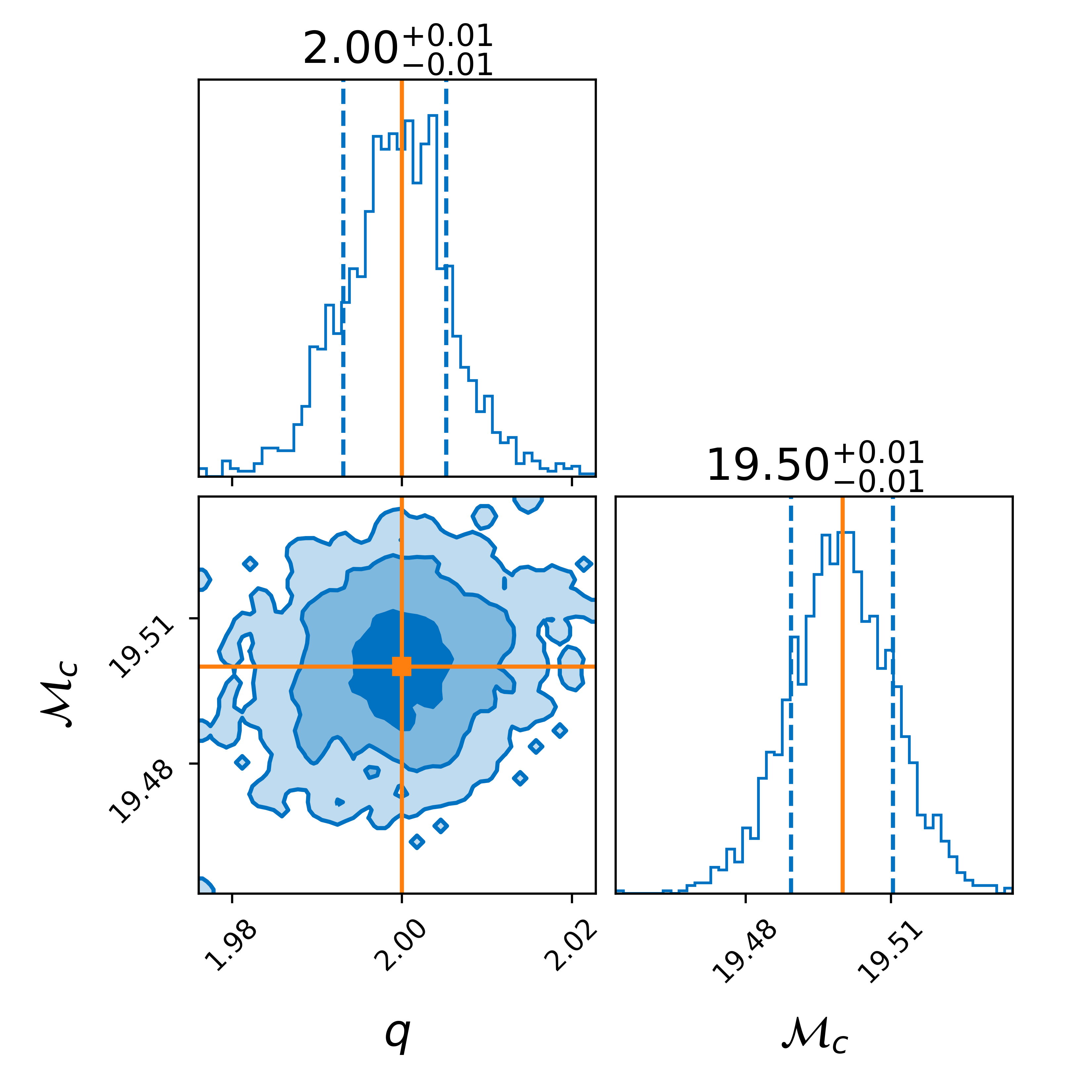
Results.—Corner plots are a visualization tool in the GW community to show the median, variance, and probability distribution for individual parameters. qBIRD allows us to generate corner plots, overlapped with the injection values or the results obtained by classical samplers. To test the quality of qBIRD simulations, we analyze a simulated GW signal constructed from Bilby [15] and PyCBC [27] injections, as shown in Figs. 3 and 4. The results represent a compromise between the largest possible problem size and the capabilities of the quantum simulator [28] on a classical computer used to obtain the results, as opposed to simulations of the LIGO collaborations obtained using HPC resources [29].

Fig. 3 shows a 2-parameter inference with qBIRD for the chirp mass $\mathcal{M}_{c}$ and mass ratio $q$ for a Gaussian-noise BBH injection through PyCBC. The priors for this inference are $\mathcal{M}_{c}\in[19.4,19.6]\ {\text{M}_{\odot}}$ and $q\in[1.9,2.1]$, using $Q=6$ discretization qubits being 6, i.e., $Q=6$, with 2000 iterations, to demonstrate the precision of the qBIRD tool. It can be seen that qBIRD performs the inference with high accuracy because it perfectly recovers the injection values $\mathcal{M}_{c}=19.50\ {\text{M}_{\odot}}$ and $q=2.00$.

As a more demanding inference, Fig. 4 shows a 4-parameter inference for the chirp mass $\mathcal{M}_{c}$, mass ratio $q$, luminosity distance $d_{L}$, and inclination angle $\theta_{jn}$ of a zero-noise BBH injection made through Bilby. In this second inference, the a prior interval has been increased considerably, $\mathcal{M}_{c}\in[25,100]\ {\text{M}_{\odot}}$, $q\in[0.25,1]$, $d_{L}\in[100,2500]\text{ Mpc}$, and $\theta_{jn}\in[0,0.8]$, and due to the limitations of the classical simulators, the discretization qubits had to be reduced to $Q=3$, with 1000 iterations. Although the inference has been significantly overcomplicated, the qBIRD algorithm is still able to reproduce the injected values $\mathcal{M}_{c}=27.43\ {\text{M}_{\odot}}$, $q=0.57$, $d_{L}=2000\text{ Mpc}$ and $\theta_{jn}=0.70$. The results are dispersion-biased due to the reduced number of qubits used for the discretization. This figure illustrates the scalability potential of qBIRD in increasing the number of parameters in the inference process. Nevertheless, the plot does not exhibit perfect convergence in parameter inference, attributed to probability oscillations around the convergence point inherent in quantum algorithms. The limited number of qubits employed in the inference, constrained by both simulator and quantum hardware limitations, contributes to this observed lack of convergence.

In SM S.IV, more technical details are provided for Figs. 3 and 4, and S.III for more results. Further, we show the inference results of parameter estimation runs for GW injections with zero-noise, GW injections with Gaussian noise, and observed data, performed using the qBIRD algorithm. Moreover, correct scalability with increasing number of parameters has been verified, approaching the limit of quantum simulators. It is crucial to emphasize that this limitation stems from classical simulators, and the algorithm exhibits full scalability when a robust quantum environment becomes feasible.

Conclusions.—We have introduced our hybrid quantum algorithm, qBIRD, for GW parameter estimation, showcasing its accuracy using the inference analysis runs for 2-parameter and 4-parameter simulated gravitational waves from BBH mergers. It builds upon the QMS framework [25] that was tested with a scaling advantage [11]. It introduces renormalization and downsampling techniques with quantum walks to realize a quantum version of the classical MCMC sampler. This method produces posteriors that closely resemble those accepted by the GW community.

The results of the corner plots with qBIRD show an accuracy in the inferred data similar to that of the classical libraries, with the dispersion being the main difference. This increase in dispersion in the quantum sampler results is due to the small number of discretization qubits and the limited number of runs to obtain the data. Classical simulators are inherently limited in the size of circuits that can be run, and the same is true for current quantum hardware, but since qBIRD is scalable, it will benefit from the upward trend of quantum advances in the near term.

Acknowledgments.— G.E., R.C. and M.A.M.-D. acknowledge the support from grants MINECO/FEDER Projects, PID2021-122547NB-I00 FIS2021, the MADQuantumCM project funded by Comunidad de Madrid, the Recovery, Transformation, and Resilience Plan, NextGenerationEU, funded by the European Union, and the Ministry of Economic Affairs Quantum ENIA project funded by Madrid ELLIS Unit CAM. H.Q. thanks Frank Linde for inspiring quantum computing exploration for gravitational wave data analysis in 2021 summer. H.Q. extends gratitude to Louisiana State University and LIGO Livingston Observatory for their hospitality during this work in 2023. M.A.M.-D. has also been partially supported by the U.S. Army Research Office through Grant No.W911NF-14-1-0103. H.Q. was supported in part by the 2022-2023 additional STFC IAA grant to Queen Mary University of London. This work used the computing facilities of the GICC group at UCM. In part the computing resources at Queen Mary University of London were supported by QMUL’s 2023 STFC IAA award. G.E. and R.C. equally contributed to this work.

^∗ gescrig@ucm.es

^† robecamp@ucm.es

^‡ hong.qi@ligo.org

^§ mardel@ucm.es

— Supplementary Materials —
Quantum Bayesian Inference with Renormalization for Gravitational Waves
Gabriel Escrig, Roberto Campos, Hong Qi, and M. A. Martin-Delgado

Appendix S.I Likelihood calculation

In General Relativity (GR), GWs are described by perturbations $h_{\mu\nu}$ of the spacetime metric as $ds^{2}=(\eta_{\mu\nu}+h_{\mu\nu})dx^{\mu}dx^{\nu}$, where $\eta_{\mu\nu}$ is the flat Minkowski reference metric. In the transverse-traceless (TT) gauge, there are only 2 independent transversal polarization modes denoted as $h_{+}$ and $h_{\times}$. The main goal of current GW detectors such as LIGO, Virgo, and KAGRA is to retrieve information on compact object coalescences from acquired data $d(t)$ during $t=1,2,\ldots,T$ data collection intervals. These data represent an observation of an event that may correspond to a binary black hole merger. To establish such correspondence, a model $M$ from GR is needed to represent the merger. When the model is faithful enough, we can obtain very useful information about intrinsic parameters of the colliding BHs such as their masses $m_{1},m_{2}$, spins $s_{1},s_{2}$ or extrinsic parameters such as their positions in the sky.

A model $M$ representing a GW signal is denoted by $h(t;\text{\boldmath$\theta$})$ where $\theta$ are the parameters characterizing the gravitational wave. This modeled signal is confronted with the experimental data $d(t)$. The model is considered faithful when the difference from the data and the signal is pure noise, namely, uncorrelated Gaussian noise $n(t)$:

$$d(t)-h(t;\text{\boldmath{\hbox{\theta}}})=n(t).$$ (S.I.1)

The signal $h(t)$ is a function of the two polarizations $h_{+}(t),h_{\times}(t)$, and the antenna patterns $F_{+},F_{\times}$,

$$h(t)=F_{+}h_{+}(t)+F_{\times}h_{\times}(t).$$ (S.I.2)

Antenna patterns depend on the detector geometry and encode the effect of the extrinsic parameters.

In the frequency domain $f_{i}$, with $i=1,2,\ldots,T$, this noise is characterized through the PSD, $S_{n}$, in the noise correlation function:

$${n}(f_{i}){n}(f_{j})=\frac{T}{2}S_{n}(f_{i})\delta_{ij},$$ (S.I.3)

where ${n}(f_{i})$ is the transformed noise distribution and $T$ the elapsed detection time.

From the statistical analysis of the data it is possible to estimate the values of the source parameters using Bayesian inference. Describing the parameter space $\bm{\theta}$ with respect to the given data ${d}(f_{i})$ and the model $M$ involves the use of PDFs denoted as $p(\bm{\theta}|d,M)$. Then, the inference of GW parameters proceeds by introducing the posterior probability by the Bayes theorem (1).

Appendix S.II Quantum Walk Operator Construction

The quantum walk operator $W=RV^{\dagger}B^{\dagger}SFBV$ (5) is composed of the following elementary operations. It starts by making a superposition over all possible movements with the $V$ operator:

$$V\ket{0}_{D}\ket{0}_{E}=\frac{1}{\sqrt{2p}}\sum_{i=0}^{p-1}\ket{i}_{D}\sum_{j\in\{0,1\}}\ket{j}_{E}=\frac{1}{\sqrt{2p}}[\ket{0}_{D}+\ket{1}_{D}+\cdots+\ket{p-1}_{D}]\otimes[\ket{0}_{E}+\ket{1}_{E}].$$ (S.II.4)

It is implemented by applying Hadamard gates to all qubits. Once all possible moves are in superposition, the acceptance probabilities (4) are encoded into the coin register with the $B$ operator:

$$B\ket{\bm{\theta}}_{S}\ket{i}_{D}\ket{\Delta\text{\boldmath{\hbox{\theta}}}_{i}}_{E}\ket{A(\bm{\theta},\bm{\theta}+\Delta\bm{\theta}_{i})}_{A}\ket{\varphi}_{C}=\ket{\bm{\theta}}_{S}\ket{i}_{D}\ket{\Delta\text{\boldmath{\hbox{\theta}}}_{i}}_{E}\ket{A(\bm{\theta},\bm{\theta}+\Delta\bm{\theta}_{i})}_{A}{\cal U}(\vartheta)\ket{\varphi}_{C},$$ (S.II.5)

where $\Delta\bm{\theta}_{i}=(0,0,\ldots,\stackrel{{\scriptstyle\text{parameter }i}}{{\Delta\theta}},\ldots,0)$, each element of the vector being a specific parameter. Implementing this operator consists of a rotation ${\cal U}(\vartheta)$ of angle $\vartheta=\arcsin\left(\sqrt{A(\bm{\theta},\bm{\theta}+\Delta\bm{\theta}_{i})}\right)$ controlled by the $\ket{A(\bm{\theta},\bm{\theta}+\Delta\bm{\theta}_{i})}_{A}$ register. At this point, the transition in the state register $\ket{\bm{\theta}}_{S}$ is performed by the $F$ operator:

$$F\ket{\bm{\theta}}_{S}\ket{i}_{D}\ket{\Delta\text{\boldmath{\hbox{\theta}}}_{i}}_{E}\ket{\varphi}_{C}=\begin{cases}\ket{\bm{\theta}}_{S}\ket{i}_{D}\ket{\Delta\text{\boldmath$\theta$}_{i}}_{E}\ket{0}_{C}&\text{if }\ket{\varphi}_{C}=\ket{0}_{C},\\ \ket{\bm{\theta}+\Delta\bm{\theta}_{i})}_{S}\ket{i}_{D}\ket{\Delta\text{\boldmath$\theta$}_{i}}_{E}\ket{1}_{C}&\text{if }\ket{\varphi}_{C}=\ket{1}_{C}.\end{cases}$$ (S.II.6)

and can be constructed from an adder gate conditioned by the coin register $\ket{\varphi}_{C}$. Then, the operator $S$ flips the sign of the value in the register $\ket{\Delta\text{\boldmath$\theta$}_{i}}_{E}$ conditioned by the coin register $\ket{\varphi}_{C}$:

$$S\ket{\bm{\theta}}_{S}\ket{i}_{D}\ket{\Delta\text{\boldmath{\hbox{\theta}}}_{i}}_{E}\ket{\varphi}_{C}=\begin{cases}\ket{\bm{\theta}}_{S}\ket{i}_{D}\ket{\Delta\text{\boldmath$\theta$}_{i}}_{E}\ket{0}_{C}&\text{if }\ket{\varphi}_{C}=\ket{0}_{C},\\ \ket{\bm{\theta}}_{S}\ket{i}_{D}\ket{-\Delta\text{\boldmath$\theta$}_{i}}_{E}\ket{1}_{C}&\text{if }\ket{\varphi}_{C}=\ket{1}_{C}.\end{cases}$$ (S.II.7)

and can be constructed from a CNOT gate controlled by the coin register $\ket{\varphi}_{C}$. Finally, the changes in the movement and coin registers are reversed and then the $\ket{0}_{P}\ket{0}_{E}\ket{0}_{C}$ state is subject to the following reflection with the $R$ operator defined as follows:

$$R\ket{i}_{D}\ket{\Delta\text{\boldmath{\hbox{\theta}}}_{i}}_{E}\ket{\varphi}_{C}=\begin{cases}-\ket{0}_{D}\ket{\text{\boldmath$0$}}_{E}\ket{0}_{C}&\text{if }(i,\Delta\text{\boldmath$\theta$}_{i},\varphi)=(0,\text{\boldmath$0$},0),\\ \ket{i}_{D}\ket{\Delta\text{\boldmath$\theta$}_{i}}_{E}\ket{\varphi}_{C}&\text{otherwise.}\end{cases}$$ (S.II.8)

Appendix S.III Extra results for qBIRD inferences

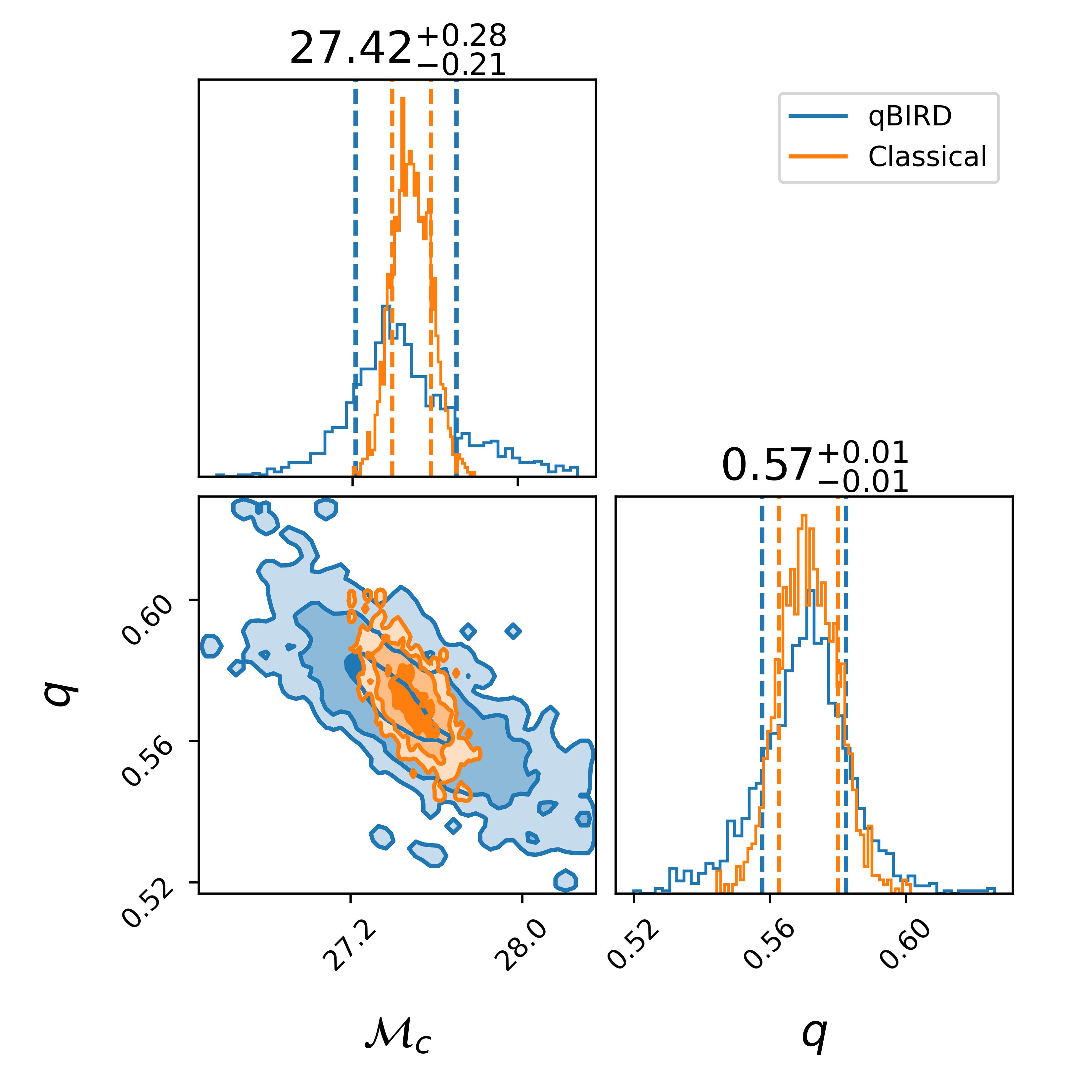
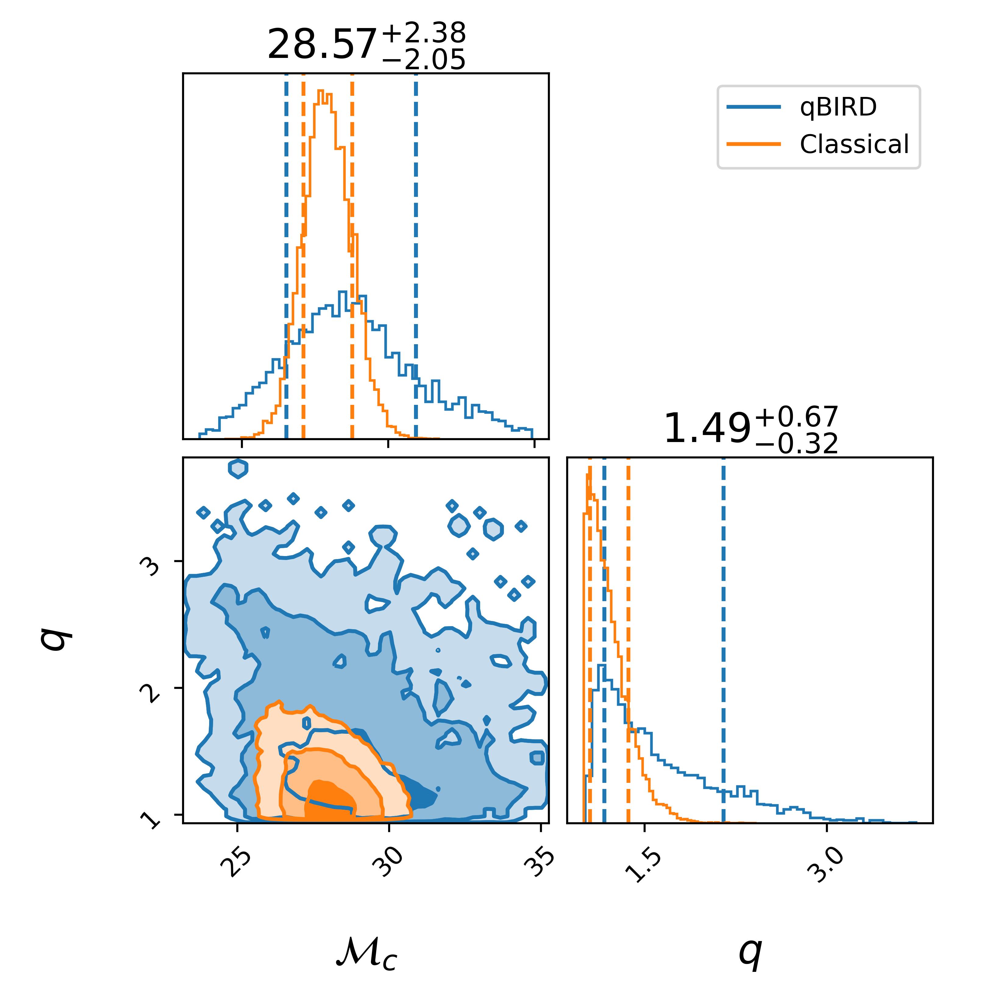
Apart from the results obtained in the main text, it can be seen that qBIRD is able to perform different types of inference, among which real data are highlighted. This section is devoted to this purpose. Technical details of the inferences can be found in S.IV.

Figure S1: Corner plots of the PDFs obtained by qBIRD for the chirp mass $\mathcal{M}_{c}$ and mass ratio $q$ for: (Left) a zero-noise BBH injection, compared to the inference of the GW library Bilby, (Right) the first detected BBH event, GW150914, compared to the GW catalog [30] from PyCBC.

Appendix S.IV Technical details for qBIRD inferences

Fig. 3 represents the posteriors obtained by qBIRD for the chirp mass $\mathcal{M}_{c}$ and the mass ratio $q$ of a simulated gaussian-noise BBH injection, calculated with the GW library PyCBC. The injection values for these inference are $\mathcal{M}_{c}=19.50\ {\text{M}_{\odot}}$ and $q=2.00$. The prior is set uniform to the intervals $\mathcal{M}_{c}\in[19.4,19.6]\ {\text{M}_{\odot}}$ and $q\in[1.9,2.1]$. Regarding the technical details of the qBIRD inference, the PDFs are constructed from 2000 iterations with a discretization of $Q=6$ qubits per parameter. This implies splitting the sample space of each parameter into $2^{6}$ points, yielding to $2^{12}$ possible configurations for $P=2$ parameters. In addition, $a=3$ qubits were used for the ancilla register, in total 18 qubits to execute the circuit. The quantum circuit has executed 4 steps $W$ in each iteration with a constant annealing schedule of $\beta=0.5$.

Fig. 4 represents the posteriors obtained by qBIRD of a 4-parameter inference of a simulated zero-noise BBH injection, calculated with the GW library Bilby. The parameters inferred are the chirp mass $\mathcal{M}$, the mass ratio $q$, the luminosity distance $d_{L}$ and the inclination angle $\theta_{jn}$. The injection values for these inference are $\mathcal{M}_{c}=27.43\ {\text{M}_{\odot}}$, $q=0.57$, $d_{L}=2000\text{ Mpc}$ and $\theta_{jn}=0.70$. The prior is set uniform to the intervals $\mathcal{M}_{c}\in[25,100]\ {\text{M}_{\odot}}$, $q\in[0.25,1]$, $d_{L}\in[100,2500]\text{ Mpc}$ and $\theta_{jn}\in[0,0.8]$. Regarding the technical details of the qBIRD inference, the PDFs are constructed from 1000 iterations with a discretization of $Q=3$ qubits per parameter. This implies splitting the sample space of each parameter into $2^{3}$ points, yielding to $2^{12}$ possible configurations for $P=4$ parameters. In addition, $a=3$ qubits were used for the ancilla register, in total 18 qubits to execute the circuit. The quantum circuit has executed 4 steps $W$ in each iteration with a constant annealing schedule of $\beta=50$.

Fig. S1 (left) represents the posteriors obtained by qBIRD for the chirp mass $\mathcal{M}_{c}$ and the mass ratio $q$ of a simulated zero-noise BBH injection, calculated with the GW library Bilby and superimposed, classical results obtained by a classical MCMC Bilby sampler. The injection values for these inference are $\mathcal{M}_{c}=27.43\ {\text{M}_{\odot}}$ and $q=0.57$. The prior is set uniform to the intervals $\mathcal{M}_{c}\in[25,100]\ {\text{M}_{\odot}}$ and $q\in[0.25,1]$. Regarding the technical details of the qBIRD inference, the PDFs are constructed from 1500 iterations with a discretization of $Q=5$ qubits per parameter. In addition, $a=3$ qubits were used for the ancilla register, in total 16 qubits to execute the circuit. The quantum circuit has executed 4 steps $W$ in each iteration with a constant annealing schedule of $\beta=500$. Classical inference has been performed with the same number of points, using the same injection values and priors with the bilby_mcmc sampler.

Fig. S1 (right) represents the posteriors obtained by qBIRD for the chirp mass $\mathcal{M}_{c}$ and the mass ratio $q$ of the real BBH event GW150914 extracted from official LIGO repositories data and superimposed, classical results obtained by the PyCBC catalog inference [31] to show the quality of the quantum inference. Regarding the technical details of the qBIRD inference, the PDFs are constructed from 1500 iterations with a discretization of $Q=5$ qubits per parameter. In addition, $a=3$ qubits were used for the ancilla register, in total 16 qubits to execute the circuit. The quantum circuit has executed 4 steps $W$ in each iteration with a constant annealing schedule of $\beta=0.5$.

Some technical information of the qBIRD algorithm is summarized in Table S1.

Table S1: Technical details of the inferences in Figures 3, 4 and S1. All quantum inferences have been generated with 4 steps of $W$ in each iteration with a constant annealing schedule and with $a=3$ ancilla qubits.

Inference	Injection Values	Prior intervals	Disc. Qubits	$\beta$ Schedule	Iterations
Fig. 3	$\mathcal{M}_{c}=19.50\ {\text{M}_{\odot}}$, $q=2.00$	$\mathcal{M}_{c}\in[19.4,19.6]\ {\text{M}_{\odot}}$, $q\in[1.9,2.1]$	$Q=6$	$\beta=0.5$	2000
Fig. 4	$\mathcal{M}_{c}=27.43\ {\text{M}_{\odot}}$, $q=0.57$, $d_{L}=2000\text{ Mpc}$, $\theta_{jn}=0.70$	$\mathcal{M}_{c}\in[25,100]\ {\text{M}_{\odot}}$, $q\in[0.25,1]$, $d_{L}\in[100,2500]\text{ Mpc}$, $\theta_{jn}\in[0,0.8]$	$Q=3$	$\beta=50$	1000
Fig. S1 (Left)	$\mathcal{M}_{c}=27.43\ {\text{M}_{\odot}}$, $q=0.57$	$\mathcal{M}_{c}\in[25,100]\ {\text{M}_{\odot}}$, $q\in[0.25,1]$	$Q=5$	$\beta=500$	1500
Fig. S1 (Right)	-	$\mathcal{M}_{c}\in[23,42]\ {\text{M}_{\odot}}$, $q\in[1,4]$	$Q=5$	$\beta=0.5$	1500

References

- Abbott et al. [2019] B. P. Abbott et al. (LIGO Scientific, Virgo), GWTC-1: A Gravitational-Wave Transient Catalog of Compact Binary Mergers Observed by LIGO and Virgo during the First and Second Observing Runs, Phys. Rev. X 9, 031040 (2019), arXiv:1811.12907 [astro-ph.HE] .
- Abbott et al. [2021] R. Abbott et al. (LIGO Scientific, Virgo), GWTC-2: Compact Binary Coalescences Observed by LIGO and Virgo During the First Half of the Third Observing Run, Phys. Rev. X 11, 021053 (2021), arXiv:2010.14527 [gr-qc] .
- Abbott et al. [2023] R. Abbott et al. (KAGRA, VIRGO, LIGO Scientific), GWTC-3: Compact Binary Coalescences Observed by LIGO and Virgo during the Second Part of the Third Observing Run, Phys. Rev. X 13, 041039 (2023), arXiv:2111.03606 [gr-qc] .
- Abbott et Al [2016] B. P. Abbott et Al (LIGO Scientific Collaboration and Virgo Collaboration), Observation of gravitational waves from a binary black hole merger, Phys. Rev. Lett. 116, 061102 (2016).
- Hall et al. [2021] E. D. Hall et al., Gravitational-wave physics with Cosmic Explorer: Limits to low-frequency sensitivity, Phys. Rev. D 103, 122004 (2021), arXiv:2012.03608 [gr-qc] .
- Punturo1, M. et al. [2010] Punturo1, M. et al., The third generation of gravitational wave observatories and their science reach, Classical and Quantum Gravity 27, 8 (2010).
- Ackley et al. [2020] K. Ackley et al., Neutron Star Extreme Matter Observatory: A kilohertz-band gravitational-wave detector in the global network, Publ. Astron. Soc. Austral. 37, e047 (2020), arXiv:2007.03128 [astro-ph.HE] .
- Kalogera et al. [2021] V. Kalogera et al., The Next Generation Global Gravitational Wave Observatory: The Science Book, (2021), arXiv:2111.06990 [gr-qc] .
- Couvares et al. [2021] P. Couvares et al., Gravitational Wave Data Analysis: Computing Challenges in the 3G Era, (2021), arXiv:2111.06987 [gr-qc] .
- Hangleiter and Eisert [2023] D. Hangleiter and J. Eisert, Computational advantage of quantum random sampling, Reviews of Modern Physics 95, 035001 (2023).
- Escrig et al. [2023] G. Escrig, R. Campos, P. A. M. Casares, and M. A. Martin-Delgado, Parameter estimation of gravitational waves with a quantum metropolis algorithm, Class. Quantum Gravity 40, 045001 (2023).
- van der Sluys et al. [2008] M. van der Sluys, V. Raymond, I. Mandel, C. Röver, N. Christensen, V. Kalogera, R. Meyer, and A. Vecchio, Parameter estimation of spinning binary inspirals using markov chain monte carlo, Classical and Quantum Gravity 25, 184011 (2008).
- Christensen et al. [2004] N. Christensen, R. Meyer, and A. Libson, A Metropolis–Hastings routine for estimating parameters from compact binary inspiral events with laser interferometric gravitational radiation data, Class. Quantum Gravity 21, 317 (2004).
- Usman et al. [2016] S. A. Usman, A. H. Nitz, I. W. Harry, C. M. Biwer, D. A. Brown, M. Cabero, C. D. Capano, T. Dal Canton, T. Dent, S. Fairhurst, et al., The pycbc search for gravitational waves from compact binary coalescence, Classical and Quantum Gravity 33, 215004 (2016).
- Ashton et al. [2019] G. Ashton, M. Hübner, P. D. Lasky, C. Talbot, K. Ackley, S. Biscoveanu, Q. Chu, A. Divakarla, P. J. Easter, B. Goncharov, et al., Bilby: A user-friendly bayesian inference library for gravitational-wave astronomy, The Astrophysical Journal Supplement Series 241, 27 (2019).
- Christensen and Meyer [2022] N. Christensen and R. Meyer, Parameter estimation with gravitational waves, Rev. Mod. Phys. 94, 025001 (2022).
- Temme et al. [2011] K. Temme, T. J. Osborne, K. G. Vollbrecht, D. Poulin, and F. Verstraete, Quantum metropolis sampling, Nature 471, 87 (2011).
- Yung and Aspuru-Guzik [2012] M.-H. Yung and A. Aspuru-Guzik, A quantum–quantum metropolis algorithm, Proceedings of the National Academy of Sciences 109, 754 (2012), https://www.pnas.org/doi/pdf/10.1073/pnas.1111758109 .
- Lemieux et al. [2020] J. Lemieux, B. Heim, D. Poulin, K. Svore, and M. Troyer, Efficient Quantum Walk Circuits for Metropolis-Hastings Algorithm, Quantum 4, 287 (2020).
- PyCBC [2021] PyCBC, Data used of 4-OGC, https://www.atlas.aei.uni-hannover.de/work/yifan.wang/4ogc/release_prod/convertsnr/1212_posterior/ (2021), [Online; accessed January-2024].
- LIGO [2016] LIGO, Data of event for GW events, https://dcc.ligo.org/public/ (2016), [Online; accessed January-2024].
- Aharonov et al. [2001] D. Aharonov, A. Ambainis, J. Kempe, and U. Vazirani, Quantum walks on graphs, in Proceedings of the thirty-third annual ACM symposium on Theory of computing (2001) pp. 50–59.
- Szegedy [2004] M. Szegedy, Quantum speed-up of markov chain based algorithms, in 45th Annual IEEE symposium on foundations of computer science (IEEE, 2004) pp. 32–41.
- Miyamoto [2023] K. Miyamoto, Quantum metropolis-hastings algorithm with the target distribution calculated by quantum monte carlo integration, Physical Review Research 5 (2023).
- Campos et al. [2023] R. Campos, P. A. M. Casares, and M. A. Martin-Delgado, Quantum metropolis solver: a quantum walks approach to optimization problems, Quantum Machine Intelligence 5, 10.1007/s42484-023-00119-y (2023).
- Wilson [1975] K. G. Wilson, The renormalization group: Critical phenomena and the kondo problem, Reviews of modern physics 47, 773 (1975).
- Nitz et al. [2024] A. Nitz, I. Harry, D. Brown, C. M. Biwer, J. Willis, T. D. Canton, C. Capano, T. Dent, L. Pekowsky, G. S. C. Davies, S. De, M. Cabero, S. Wu, A. R. Williamson, B. Machenschalk, D. Macleod, F. Pannarale, P. Kumar, S. Reyes, dfinstad, S. Kumar, M. Tápai, L. Singer, P. Kumar, veronica villa, maxtrevor, B. U. V. Gadre, S. Khan, S. Fairhurst, and A. Tolley, gwastro/pycbc: v2.3.3 release of pycbc (2024).
- ANIS et Al [2021] M. S. ANIS et Al, Qiskit: An open-source framework for quantum computing (2021).
- Canizares et al. [2015] P. Canizares, S. E. Field, J. Gair, V. Raymond, R. Smith, and M. Tiglio, Accelerated gravitational wave parameter estimation with reduced order modeling, Physical review letters 114, 071104 (2015).
- Nitz et al. [2023a] A. H. Nitz, S. Kumar, Y.-F. Wang, S. Kastha, S. Wu, M. Schäfer, R. Dhurkunde, and C. D. Capano, 4-ogc: Catalog of gravitational waves from compact binary mergers, The Astrophysical Journal 946, 59 (2023a).
- Nitz et al. [2023b] A. H. Nitz, S. Kumar, Y.-F. Wang, S. Kastha, S. Wu, M. Schäfer, R. Dhurkunde, and C. D. Capano, 4-OGC: Catalog of gravitational waves from compact binary mergers, Astrophys. J. 946, 59 (2023b).