Offline Fictitious Self-Play for Competitive Games

Abstract

Offline Reinforcement Learning (RL) has received significant interest due to its ability to improve policies in previously collected datasets without online interactions. Despite its success in the single-agent setting, offline multi-agent RL remains a challenge, especially in competitive games. Firstly, unaware of the game structure, it is impossible to interact with the opponents and conduct a major learning paradigm, self-play, for competitive games. Secondly, real-world datasets cannot cover all the state and action space in the game, resulting in barriers to identifying Nash equilibrium (NE). To address these issues, this paper introduces Off-FSP, the first practical model-free offline RL algorithm for competitive games. We start by simulating interactions with various opponents by adjusting the weights of the fixed dataset with importance sampling. This technique allows us to learn best responses to different opponents and employ the Offline Self-Play learning framework. In this framework, we further implement Fictitious Self-Play (FSP) to approximate NE. In partially covered real-world datasets, our methods show the potential to approach NE by incorporating any single-agent offline RL method. Experimental results in Leduc Hold’em Poker show that our method significantly improves performances compared with state-of-the-art baselines.

1 Introduction

Multi-agent reinforcement learning (MARL) provides a powerful learning framework to tackle the problems in multi-agent systems and has been applied to a wide range of domains, such as Go (Silver et al., 2017), strategy games (Vinyals et al., 2019), robotics (Yu et al., 2023), unmanned aerial vehicle (Yun et al., 2022) and network routings (Ye et al., 2015). MARL requires extensive interaction and exploration with accurate and efficient environments, however, this requirement is often not fulfilled in practice, such as football (Kurach et al., 2020), negotiation (Yang et al., 2020), wildlife security protection (Fang et al., 2016), and crowdsourcing (Gerstgrasser et al., 2021). The existing data-driven method, supervised learning, also called behavior cloning, heavily relies on high-quality datasets, which are commonly expensive and suboptimal. Offline MARL offers an excellent alternative to solve these issues by improving policies from previously collected datasets without further interactions (Tseng et al., 2022; Yang et al., 2021).

Recent research in offline MARL has predominantly concentrated on cooperative tasks, where all agents receive a common reward. For cooperative tasks, the goal can be seen as maximizing the cumulative rewards of a joint policy of all agents. Thus, existing single-agent offline RL methods can be easily extended to multi-agent scenarios  (Tseng et al., 2022). However, competitive tasks, often framed as zero-sum games, necessitate a divergent goal orientation.

In the realm of competitive games, or called zero-sum games, exemplified by Texas hold’em poker in studies by (Brown & Sandholm, 2018, 2019), the pursuit of a Nash equilibrium emerges as a prevalent solution concept. Complementary efforts in online setting by (Silver et al., 2017; Ye et al., 2020) focus on the ELO ratio or returns. To reach these goals, These approaches predominantly rely on the self-play paradigm, wherein policies are continuously refined to maximize returns against evolving adversary policies. Nonetheless, in the offline scenario, self-play doesn’t work due to the absence of online interactions, complicating the development of effective offline learning algorithms for competitive games.

In addressing competitive games, recent benchmarks such as AlphaStar Unplugged (Mathieu et al., 2023) and Hokoff (Qu et al., 2023; Wei et al., 2022) have applied single-agent offline RL algorithms to multi-agent settings. However, maximizing the cumulative rewards against static opponents results in an overfitting policy and vulnerable exploitation by more dynamic opponents. Moreover, when datasets are collected by poor policies, such as random policies, it is pointless to learn to defeat these weak opponents, because real-life opponents typically exhibit rational and high-performance behaviors. Li et al. (2022) proposes a model-based offline paradigm for equilibrium finding but requires a strong assumption that datasets fully cover the state-action space of original games. Cui & Du (2022a); Zhong et al. (2022); Cui & Du (2022b) contribute to theoretical insights for a weaker assumption on datasets but only propose algorithms that are feasible in theory. These works encounter challenges in integration with single-agent offline RL methods and do not offer a practical algorithm for addressing real-world problems.

In this paper, we proposed an offline learning framework, called Offline Self-Play (Off-SP), and an offline learning algorithm, Offline Fictitious Self-Play (Off-FSP), for equilibrium finding in zero-sum extensive-form games, bridging the gap between single-agent offline RL and competitive games. To our knowledge, Off-FSP is the first model-free offline algorithm for practical zero-sum game that offers the flexibility to combine with various Offline RL agents. We first propose a technique to approximate interaction with different opponents by re-weighting the datasets with importance sampling. This allows us to learn the best responses against arbitrary opponents with offline RL and derives self-play under the offline setting. By implementing the fictitious self-play on Off-SP, Off-FSP acquires the ability to learn strategies that approximate NE using fixed datasets. We also discuss the challenges of missing data for real-world datasets. The experiments in an imperfect-information two-player zero-sum game, Leduc Hold’em Poker, show that our method outperforms the state-of-the-art baselines and can approach a Nash equilibrium in datasets that fully cover the state-action space of the game. Even with partially covered datasets, our methods show the ability to reduce exploitability in original games.

2 Related Work

In competitive games, also known as zero-sum games, people have developed a series of learning algorithms, where finding Nash equilibrium with self-play is the major learning paradigm for this problem. Fictitious self-play (FSP) (Heinrich et al., 2015) combines fictitious play (FP) (Brown, 1951) with self-play and provably converges to an NE in extensive-form games. Counterfactual regret minimization (CFR) (Bowling et al., 2015) combines regret minimization with self-play, first solving an imperfect-information game of real-world scale. DeepNash (Perolat et al., 2022) extends regularised Nash dynamics with RL and converges to an approximate NE in Stratego. Policy-Space Response Oracles (PSRO) (Lanctot et al., 2017) learn to find NE by iteratively learning best responses to its policies’ population, which can also be seen as a population-based self-play. Some works (Silver et al., 2017; Ye et al., 2020; Yang et al., 2022) of large-scale games aim for a higher winning percentage or returns and try to exploit opponents, not pursuing strict NE, still based on the self-play paradigm.

In the offline learning paradigm, behavior cloning (BC) is the simplest form that directly imitates the sampling strategy of datasets. The performance of BC is limited by the sampling strategy in the dataset, while offline RL can surpass this limitation by maximizing returns. Offline RL faces the challenge of the extrapolation error on out-of-distribution states and actions. Batch-constrained deep q-learning (BCQ) (Fujimoto et al., 2019b) and conservative q-learning (CQL) (Kumar et al., 2020) mitigate this issue by constraining the gap between policy and data distribution. Critic regularized regression (CRR) (Wang et al., 2020) solve this problem by weighted behavior cloning.

In offline competitive scenarios, BC is a viable algorithm, still limited by the quality of sampling strategy in datasets. Mathieu et al. (2023); Qu et al. (2023) directly learn strategies by single-agent offline RL without self-play. This way also requires high-quality behavior strategies in datasets and is easily overfitted to fixed opponents. Cui & Du (2022a); Zhong et al. (2022); Cui & Du (2022b) propose theoretically feasible algorithms. Li et al. (2022) proposed a model-based learning framework, OEF, for extending online equilibrium-finding algorithms in offline scenarios. However, OEF only supports datasets with full coverage of state-action spaces, which is not realistic for real-world problems. Although previous theoretic methods allow for partially covered datasets, they cannot be practically applied to real-life problems. In this paper, Off-SP enables the self-play paradigm in offline MARL of competitive games. Off-FSP implement a practical algorithm to find NE and has the potential to learn on partially covered datasets by integrating any variants of single-agent offline RL algorithms.

3 Preliminaries

3.1 Extensive-form Game

Extensive-form games are a model of sequential interaction involving $n$ agents. Each player’s goal is to maximize his payoff in the game. At each step $t$ of extensive-form game, only one player observes his respective information states $s^{i}_{t}\in\mathcal{S}^{i}$ and suggests his action $a^{i}_{t}\in\mathcal{A}^{i}(s^{i}_{t})$. $\mathcal{S}^{i}$ is the set of information states of player $i$, and $\mathcal{A}^{i}(s)$ is the set of aviliable action at state $s$. The game’s randomization is defined by an extra player $c$, called chance. Chance follows a fixed randomized strategy that determines the distribution of the next state at its turns. The player function $P:\mathcal{S}\rightarrow\mathcal{N}\cup\{c\}$, with $\mathcal{N}=\{1,\dots,n\}$ denotes the set of players, determines who is to act at a given state.

We assume the games with perfect recall. Each player’s current information state $s_{t}^{i}$ implies the trajectory sequence $(s_{1}^{i},a_{1}^{i},s_{2}^{i},a_{2}^{i},\dots,s_{t}^{i})$, including information states and actions led to $s_{t}^{i}$. In extensive-form games, each player plays following a behavioural strategy that maps all information states to distributions of available actions. The realization-plan (Von Stengel, 1996), $x(s_{t}^{i})=\Pi_{j=1}^{t-1}\pi^{i}(a_{j}^{i}|s_{j}^{i})$, describes the probability of reaching the information state $s_{t}^{i}$ following player $i$’s behavioural strategy, $\pi^{i}$. The strategy profile $\pi=(\pi^{1},\dots,\pi^{n})$, is a joint of all player’s behavioural strategy. $\pi^{-i}$ denotes the strategy profile of all players excepts $i$. The payoff of player $i$ is denoted by $R^{i}(\pi^{i},\pi^{-i})\in\mathbb{R}$, and $\sum_{i}R^{i}=0$ for zero-sum games. Given a fixed $\pi^{-i}$, best response $\textsc{BR}(\pi^{-i})$ is the strategy that has the highest payoff. A Nash equilibrium (NE) is a strategy profile that any strategy $\pi^{i}$ in this profile is a best response to the opponent’s profile $\pi^{-i}$. The $\epsilon$-best response ($\epsilon$-BR) and $\epsilon$-Nash equlibirium ($\epsilon$-NE) are approximations to above defination. $\epsilon$-BR is suboptimal by no more than $\epsilon$ compared with BR. Similarly, $\epsilon$-NE is a profile of $\epsilon$-BR. NashConv (Timbers et al., 2022), also called exploitability in two-player zero-sum games, evaluates the distance from $\pi$ to an NE, defined as $\sum_{i}R^{i}(\textsc{BR}(\pi^{-i}),\pi^{-i})-R^{i}(\pi^{i},\pi^{-i})$.

Normal-form game is a simplified game description in game theory. Normal form represents the game by way of a matrix. An extensive-form game induces an equivalent normal-form game. In Sections 4.4 and 5.1, we discuss with toy examples of a normal-form game, rock-paper-scissors, and show the experimental results.

Algorithm 1 Fictitious Self-Play

Function FictitiousSelfPlay()

      Initialize strategy $\pi_{0}$.  for $k=1$ to $K$ do

           $\mathcal{D}_{k}\leftarrow$ GenerateData($\pi_{k-1}$) foreach player $i\in\mathcal{N}$ do

                $\beta^{i}_{k}\leftarrow$ LearnBestResponse($\mathcal{D}_{k},\pi^{-i}_{k-1}$)

          $\pi_{k}\leftarrow$ UpdateAverageStrategy($\pi^{i}_{k-1},\beta^{1}_{k},\dots,\beta^{n}_{k}$)

     return average strategy $\pi_{K}$ 

3.2 Fictitious Self-Play

Fictitious Play (Brown, 1951) is a game-theoretic model for learning from self-play. Fictitious players iteratively compute the best responses to opponents’ average behavioural strategy and update their set of strategies. The average strategies of fictitious players are proven to converge to Nash equilibria in two-player zero-sum and many-player potential games. Generalised weakened fictitious play (Leslie & Collins, 2006) is an improvement of fictitious play that enables approximate best responses and perturbed average strategy updates. Generalised weakened fictitious play also provably converges to Nash equilibria in certain game classes and is suitable for machine learning framework.

Original fictitious Play is defined in normal-form games, which requires exponential computations for extensive-form games. Heinrich et al. (2015) introduce Fictitious Self-Play (FSP) that extend fictitious play and generalised weakened fictitious play into the extensive-form game with linear time and space complexity. We briefly describe FSP at  Algorithm 1. In extensive-form games, the average strategies $\pi^{i}_{k}$ are updated by the realization-equivalence theorem. At the $k$-th iteration of FSP, the average behavioural strategy of player $i$ is

$$\begin{split}\forall s,a:~{}&\pi^{i}_{k}(a|s)=(1-\lambda)\pi^{i}_{k-1}(a|s)+\lambda\beta^{i}_{k}(a|s),\\ &\lambda=\frac{\alpha_{k}x_{\beta^{i}_{k}}(s)}{(1-\alpha_{k})x_{\pi^{i}_{k-1}}(s)+\alpha_{k}x_{\beta^{i}_{k}}(s)},\end{split}$$ (1)

where $\beta^{i}_{k}\in\epsilon_{k}\textsc{-BR}(\pi_{k-1}^{-i})$ is a best-response to opponent $\pi_{k-1}^{-i}$ and $\alpha_{k}$ is parameter to mix the best-response $\beta^{i}_{k}$ and previous average strategy $\pi^{i}_{k-1}$. Strategy $\pi^{i}_{k}$ is equivalent to choosing either strategy $\pi^{i}_{k-1}$ or $\beta^{i}_{k}$ before the beginning of each game, with probabilities $1-\alpha_{k}$ and $\alpha_{k}$ respectively. When $\alpha_{k}\rightarrow 0$ and $\epsilon_{k}\rightarrow 0$ as $k\rightarrow 0$, and $\sum_{k=1}^{\infty}\alpha_{t}=\infty$ for all $n$ players, the average strategy profile $\pi_{k}=(\pi^{1}_{k},\dots,\pi^{n}_{k})$ converge to an NE. In a common setting with $\alpha_{k}=\frac{1}{k}$, $\pi_{K}^{i}$ is equivalent to choosing all strategy $\beta^{i}_{1},\dots,\beta^{i}_{K}$ with the probability of $\frac{1}{K}$. The update of average behavioural strategy requires a traverse for all information state $s^{i}\in\mathcal{S}^{i}$, which is computationally expensive for large games and machine learning-based frameworks. FSP restored all the data of strategies $\beta^{i}_{1},\dots,\beta^{i}_{k}$ and trained an approximate average strategy with supervised learning.

3.3 Offline Reinforcement Learning

(a) Off-FSP and Off-SP.

(b) Differences between FSP and Off-FSP.

Figure 1: Illustration of Off-FSP, Off-SP and three essential functions. The green box in (a) is the Off-SP.

Reinforcement learning (RL) agents aim to maximize the expected cumulative discounted reward in a Markov decision process (MDP). MDP is denoted as a tuple $\mathcal{M}=(\mathcal{S},\mathcal{A},\mathcal{T},\rho_{0},r,\gamma,T)$. $\mathcal{S},\mathcal{A}$ represent the state and action spaces. $\mathcal{T}(s_{t+1}|s_{t},a_{t}),r(s_{t},a_{t})$ represent the dynamics and reward function. $\rho_{0}$ is the distribution of initial state $s_{1}\sim\rho_{0}$. $\gamma\in[0,1]$ is the discount factor. Many reinforcement learning algorithms learn from transition tuples, $(s_{t},a_{t},r_{t},s_{t+1})$, where $s_{t},a_{t},r_{t}$ are the state, action and reward at time $t$, and $s_{t+1}$ is the next state after agent take action $a_{t}$ at state $s_{t}$. The expected cumulative discounted reward following policy $\pi$ can be formalized as the action-value function $Q(s_{t},a_{t})=\mathbb{E}_{\pi}[\sum^{\infty}_{i=t}\gamma^{i-t}r(s_{i},a_{i})]$. Model-based RL methods learn the dynamic models while model-free methods directly learn the Q function to state-action pairs. Given the fixed opponent $\pi_{-i}$ and an extensive form game, the game of player $i$ can be defined as a MDP $\mathcal{M}(\pi_{-i})$ (Silver & Veness, 2010; Greenwald et al., 2013). Player $i$’s information state defines the state, and his payoff function defines the reward. An $\epsilon$-optimal policy of the MDP, $\mathcal{M}(\pi^{-i})$, is also the $\epsilon$-BR to the strategy $\pi^{-i}$.

Offline RL algorithm breaks the assumption that the agent can interact with the environment. The offline RL algorithm learns to maximize the expected cumulative reward based on a fixed dataset. The dataset is sampled following a behavior policy $\pi_{b}(a|s)$ in MDP $\mathcal{M}$. $\hat{\pi}_{b}(a|s):=\frac{\sum_{s,a\in\mathcal{D}^{i}}\mathbbm{1}[s=s,a=a]}{\sum_{s\in\mathcal{D}^{i}}\mathbbm{1}[s=s]}$ denote the empirical behavior policy, at all state $s\in\mathcal{D}^{i}$. In offline RL, the Q-function is trained only on actions sampled from offline datasets, which cannot cover all state and action spaces. Therefore, the Q-function may be erroneously overestimated at out-of-distribution (OOD) actions, which is called extrapolation error (Fujimoto et al., 2019b). Recent offline RL methods encourage the policy to learn on the support of training data or employ weighted behavior cloning to mitigate this error.

4 Offline Fictitious Self-Play

In this section, we introduce the Offline Self-Play (Off-SP) learning framework and give an implementation as Offline Fictitious Self-Play (Off-FSP) algorithm to find an $\epsilon$-Nash equilibrium with a fixed dataset. In the online scenario, self-play is a process in which a strategy iteratively maximizes cumulative rewards against itself, and fictitious self-play plays against the average of its past strategies. Corresponding to the concept of the online setting, Off-SP is a learning framework that enables strategy play against changing opponents with a fixed dataset. Off-FSP implement fictitious self-play on this learning framework with average strategies as the changing opponents and learn to find NE.

Initially, we describe the offline datasets and make strong assumptions to simplify the problem. Based on the original FSP, as described in Algorithm 1, we derive the offline fictitious self-play by replacing three essential functions. In Section 4.2, we replace GenerateData by simulating play against different opponents with weighted datasets and replace LearnBestResponse with single-agent offline RL algorithm. The first two functions introduce Off-SP. In Section 4.3, we replace UpdateAverageStrategy by computing the average strategy based on samples and derive Off-FSP. Lastly, we discuss how offline RL helps Off-FSP to reduce the exploitability under real-world datasets.

4.1 Assumptions of Offline Datasets

Trajectory and Dataset.

The trajectory of extensive-form games is a sequence of information states, actions, and player’s id. The trajectory also involves states and actions of chance $c$. The trajectory $\tau_{E}=\{s_{1},a_{1},p_{1},s_{2},\dots,s_{T},a_{T},p_{T}\mid p_{t}=P(s_{t})\},$

We can assume the next information state for a prefix of trajectory and the payoff for a whole trajectory are definite. In other words, if we know the information sets of all players and chance, the game is deterministic.

In player $i$’s perspective, the extensive-form game can be modeled as an MDP $\mathcal{M}$ given a fixed opponent $\pi^{-i}$ (Silver & Veness, 2010; Greenwald et al., 2013). In MDP $\mathcal{M}$, the dynamic function $\mathcal{T}(s^{i}_{t+1}\mid s^{i}_{t},a^{i}_{t})$ models the dynamics of opponents and the chance player. The observed MDP is non-deterministic because of imperfect information in a single player’s information state.

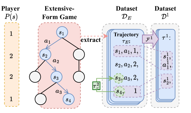
To learn best-response with single-agent RL, we project the trajectory $\tau_{E}$ into player $i$’s perspective with a projection function $\tau^{i}=\mathcal{F}^{i}(\tau_{E})$. The projection $\mathcal{F}^{i}$ filters out the states corresponding to player $i$ while relabeling the time indices.

$$\begin{split}\tau^{i}&=\mathcal{F}^{i}(\tau_{E})=\{s_{t},a_{t}\mid\forall p_{t}\in\tau_{E},p_{t}=i\}\\ &=\{s_{1}^{i},a_{1}^{i},s_{2}^{i},\dots,s_{T^{\prime}}^{i},a_{T^{\prime}}^{i}\},\end{split}$$

where $T^{\prime}$ is the length of the player $i$’s trajectory $\tau^{i}_{\mathcal{M}}$. The subscripts of $s_{t}$ and $s_{t}^{i}$ are different and represent the time indices in the corresponding trajectories. For state $s^{i}_{t}\in\tau^{i}_{\mathcal{M}}$, we use function $I(s^{i}_{t})$ to denote the subscript of state in $\tau_{E}$. We denote opponent $j$’s latest state at player $i$’s state $s_{t}^{i}$ with function $\tau_{<}^{j}(s_{t}^{i})$.

$$\tau_{<}^{j}(s_{t}^{i})=s_{k},~{}\text{where}~{}{k=\max\{k^{\prime}<I(s^{i}_{t})\mid p_{k^{\prime}}=j\}}.$$

In order to offer a clear explanation of the stated components, we present an example trajectory in Figure 2.

Figure 2: An example of extensive-form games and datasets. (Left) An example trajectory in extensive form game; (Right) Illustration of trajectories and dataset in extensive-form game and single-agent perspective. The orange area represents the player function. Blue parts represent the trajectories. The purple area represents the projection relationship under function $\mathcal{F}^{1}$. The green parts explain how function $\tau^{2}_{<}$ works.

Based on the description of trajectory in both extensive-form games and single-agent perspective, the datasets consist of multiple corresponding trajectories. For extensive-form game, the dataset is $\mathcal{D}_{E}=\{\tau_{E}\}$. The dataset for player $i$ is $\mathcal{D}^{i}=\{\tau^{i}_{\mathcal{M}}=\mathcal{F}^{i}(\tau_{E})\mid\tau_{E}\in\mathcal{D}_{E}\}$. The $i$-th player’s dataset, derived from dataset $\mathcal{D}_{E}$, is denoted as $\mathcal{D}^{i}=\mathcal{F}^{i}(\mathcal{D}_{E})$. For briefly, we ignore the reward transformation in trajectories.

Assumptions for Offline Learning.

To introduce our method, we first assume the offline dataset $\mathcal{D}_{E}$ is both a fully covered dataset and a real-equivalence dataset. This assumption, crucial for the theoretical derivation of our methods, is not a prerequisite for practical application. The adaptability of our method to real-world datasets, unconstrained by these assumptions, is discussed in Section 4.4. The definitions of these two concepts are provided as follows.

Definition 4.1 (Fully Covered Dataset).

$\mathcal{S}\text{~{}and~{}}\mathcal{A}$ represent the joint sets of information states and actions for all players $\mathcal{N}\cup\{c\}$. A dataset $\mathcal{D}_{E}$ in extensive-form games is a fully covered dataset if $\forall s\in\mathcal{S},a\in\mathcal{A}(s)\Rightarrow(s,a)\in\mathcal{D}_{E}$.

When a dataset is fully covered, the trained learning algorithm will not suffer from OOD problems.

Definition 4.2 (Real-Equivalence Dataset).

For a dataset of extensive-form game $\mathcal{D}_{E}$ sampled following a behavior strategy $\pi_{b}$, dataset $\mathcal{D}_{E}$ is an real-equivalence dataset if $Pr(\tau_{E})=\frac{\sum_{\tau\in\mathcal{D}_{E}}\mathbbm{1}[\tau=\tau_{E}]}{|\mathcal{D}_{E}|},\forall\tau_{E}\in\mathcal{D}_{E},$ where $Pr(\tau_{E})$ is the probability of sampling trajectory $\tau_{E}$ with $\pi_{b}$ online.

When a dataset is a real-equivalence dataset , sampling trajectories from the offline dataset $\mathcal{D}_{E}$ is equivalent to sampling from the extensive-form game with strategy $\pi_{b}$ online and the right-hand side of the equation is the probability density of $\tau_{E}$ in $\mathcal{D}_{E}$, denoted by $\mathcal{D}_{E}(\tau_{E})$.

4.2 Learning Open-ended Best-Response

Self-play and fictitious self-play iteratively interact with the game to generate data and utilize the data to learn best responses. In $k$-th iteration, the opponent for player $i$ is changed to $\pi^{-i}_{k-1}$, therefore, in order to learn the best response $\beta^{i}_{k}=\text{BR}(\pi^{-i}_{k-1})$, player $i$ must interact with $\pi^{-i}_{k-1}$ to generate new data $\mathcal{D}^{i}_{k}$. The process, from the perspective of player $i$, is equivalent to interacting with a new MDP $\mathcal{M}(\pi^{-i}_{k})$ and maximizing returns with RL to learn the corresponding best response (Greenwald et al., 2013).

In offline settings, we are limited to using a fixed dataset sampled by behavioural policy $\pi_{b}$, in which RL methods can only obtain the best response $\text{BR}(\pi_{b}^{-i})$ for player $i$. In order to execute the fictitious self-play, we should generate player $i$ datasets under different MDP $\mathcal{M}(\pi^{-i}_{k})$. With importance sampling (Nachum et al., 2019), we can emulate sampling from another dataset $\mathcal{D}^{i}_{w}$ with weighting $w(d_{t})=\frac{\mathcal{D}^{i}_{w}(d_{t})}{\mathcal{D}^{i}(d_{t})}$ (Hong et al., 2023) on the original dataset $\mathcal{D}^{i}$, where $\mathcal{D}^{i}_{w}(d_{t})$ and $\mathcal{D}^{i}(d_{t})$ denote the probability density of tuple $d_{t}=(s^{i}_{t},a^{i}_{t},s^{i}_{t+1})$ in according datasets. This formulation gives the following equivalence:

$$\mathbb{E}_{d_{t}\sim\mathcal{D}^{i}_{w}}[L(d_{t};\theta)]\Leftrightarrow\mathbb{E}_{d_{t}\sim\mathcal{D}^{i}}[w(d_{t})L(d_{t};\theta)],$$ (2)

where $L(d_{t};\theta)$ is the loss function of an off-policy RL method, and $\theta$ is the parameter of RL policy to be optimized. With the assumption that dataset $\mathcal{D}_{E}$ is both a fully covered dataset and a real-equivalence dataset, sampling from it with importance sampling is equivalent to sampling from the online game with importance sampling.

Theorem 4.3.

For player $i$, the weight of transferring opponent from $\pi^{-i}_{b}$ to $\pi^{-i}$ is:

$$w(d_{t})=\frac{x^{-i}_{\pi^{-i}}(s_{j}){\pi^{-i}}(a_{j}|s_{j})}{x^{-i}_{\pi_{b}^{-i}}(s_{j}){\pi_{b}^{-i}}(a_{j}|s_{j})},~{}s_{j}=\tau_{<}^{-i}(s_{t+1}^{i}).$$ (3)

In order to simplify the phrase, we denote the strategies of $n-1$ opponents as an ensemble strategy $\pi^{-i}$ and refer to them as player $-i$. The proof of Theorem 4.3 is provided in Appendix A. Given an offline dataset $\mathcal{D}_{E}$, the behavior strategy $\pi_{b}$ can be approximated by an empirical behavioural policy $\tilde{\pi}_{b}$. In extensive-form games, we can estimate $\tilde{\pi}_{b}$ by counting or supervised learning policy.

When considering a particular opponent, the weight $w(d_{t})$ assigned to a sample $d_{t}$ may shift to zero or a large value. As a result, when training RL with batched samples, the RL loss suffers from a large variance (Munos et al., 2016), leading to unstable training. To address this issue, we employ $\frac{w(d_{t})}{\sum_{d\in\mathcal{D}}w(d)}$ as the sampling probability rather than multiply the loss function by $w(d_{t})$ as shown in Equation 2. In this way, re-sampling from fully covered real-equivalence datasets is identical to sample data in online games. With batches of data sampled from the dataset, we can apply an offline RL to learn best responses.

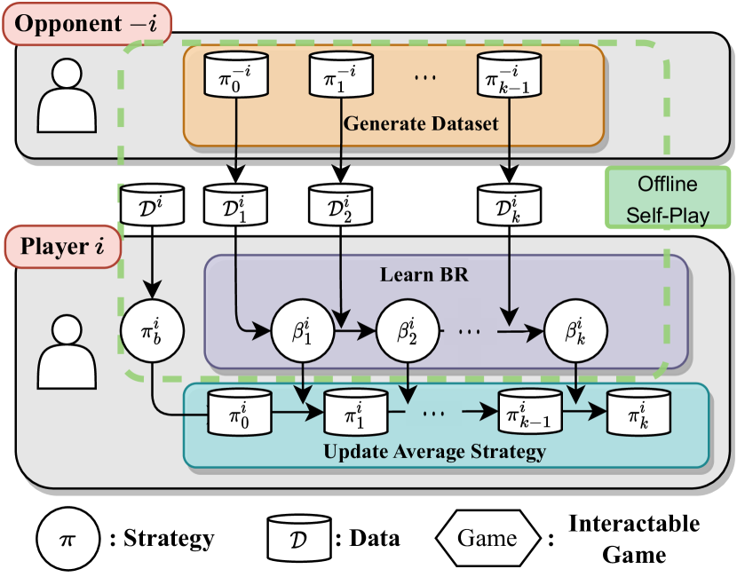
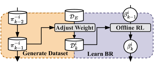
Figure 1(b) and Figure 3 illustrates these two functions and Off-SP. In the function GenerateDataset, we first calculate $w(d)$ for all the samples $d_{t}$ and get a re-weighted dataset $\mathcal{D}_{k}^{i}$ for each player $i$. In the function LearnBestResponse, offline RL algorithms repeatedly sample a batch of data and optimize the learned policy for $M$ times. These two functions derive the Off-SP. At each step $t$, Off-SP first generates dataset play against the current opponents and updates strategies towards the best response of the opponents.

Figure 3: Offline Self-Play learning framework.

4.3 Aggregate Average Strategy in Samples

Before diving into Off-FSP, it is essential to review the mechanics of fictitious play in an online scenario. In norm-form games, fictitious play updates the new average strategy $\pi_{k+1}$ following Equation 1 after learning the best responses. To extend FP on extensive-form games, FSP gathers the trajectories of $\beta^{i}_{k}$ during each iteration and employs supervised learning to approximate $\pi^{i}_{k+1}$ for each player. However, Off-FSP does not require the current average strategy $\pi_{k}$ to sample new data, but only requires probability $\pi_{k}(s,a)$ for all state-action pairs in a fixed dataset. Therefore, an interactable average strategy $\pi_{k}$ is not necessary. We can just maintain the probability $\pi_{k}(s,a)$ in the datasets for the weighting technique. Traverse along the trajectory $\tau_{i}$, Off-FSP computes the probability $\pi^{i}_{k}(s,a)$ for player $i$ following Equation 1. Figure 1(b) shows one step of the function UpdateAverageStrategy. To facilitate the calculation, we save the probability into the current dataset $\mathcal{D}^{i}_{k}$, changing the sample into $d^{\prime}=(s,a,\pi^{i}_{k}(s,a))$.

Although the weighting technique does not require a real instance of average behavioural strategy, Off-FSP requires an interactable strategy as output. One way is utilizing supervised learning to imitate the behavioural strategy with the weighting technique. When the dataset is not a fully covered dataset, this restricts strategies to exclusively choosing actions that are present in the dataset. In our experiments, we opted for an alternative method that involves aggregating all policies within a collection $\Pi$. Before the beginning of each game, one of the strategies in $\Pi$ is chosen with a specific probability and the payoff of the aggregation is the expectative payoff over all possible strategies. This approach maintains the option of picking actions that are out of the distribution but necessitates a larger storage capacity for storing all strategies. Algorithm 2 and Figure 1(a) present the pipeline of Offline Fictitious Self-play.

Algorithm 2 Offline Fictitious Self-Play

Function Off-FictitiousSelfPlay($\mathcal{D}_{E}$):

      Estimate the empirical behavioural policy $\tilde{\pi}_{b}$  $\Pi_{i}\leftarrow\{\pi_{b}^{i}\},\quad\pi_{0}\leftarrow\tilde{\pi}_{b}$  $\mathcal{D}^{i}_{0}\leftarrow\{(s,a,\pi^{i}_{0}(s,a))|(s,a)\in\mathcal{F}^{i}(\mathcal{D}_{E})\}$  for $k=1$ to $K$ do

           for each player $i\in\mathcal{N}$ do

                $\mathcal{D}^{i}_{k}\leftarrow$ GenerateDataset($\mathcal{D}_{E},\mathcal{D}^{-i}_{k-1}$) $\beta^{i}_{k}\leftarrow$ LearnBestResponse($\mathcal{D}^{i}_{k},\beta^{i}_{k-1}$) $\mathcal{D}^{i}_{k}\leftarrow$ UpdateAverageStrategy($\mathcal{D}^{i}_{k-1},\beta_{k}^{i}$) Update collection of BRs $\Pi_{i}\leftarrow\Pi_{i}\cup\{\beta_{k}^{i}\}$ 

     return Aggregate($\Pi$)

Function GenerateDataset($\mathcal{D}_{E},\mathcal{D}^{-i}_{k-1}$):

      Get probability of $\pi_{k-1}^{-i}$ from $\mathcal{D}^{-i}_{k-1}$  Calculate $w_{\pi_{k-1}^{-i}}$ following Equation 3  $\mathcal{D}^{i}_{k}\leftarrow$ WeightData($\mathcal{D}_{E},w_{\pi_{k}^{-i}}$)  return $\mathcal{D}^{i}_{k}$

Function LearnBestResponse($\mathcal{D}^{i}_{k},\beta^{i}_{k-1}$):

      Initialize policy parameters with $\beta^{i}_{k}\leftarrow\beta^{i}_{k-1}$  Optimize $\beta^{i}_{k}$ with offline RL and data $\mathcal{D}^{i}_{k}$  return $\beta^{i}_{k}$

Function UpdateAverageStrategy($\mathcal{D}^{i}_{k-1},\beta^{i}_{k}$):

      for $(s,a,\pi_{k-1}^{i}(s,a))\in\mathcal{D}^{i}_{k-1}$ do

           Calculate $\pi_{k}^{i}(s,a)$ with $\beta^{i}_{k},\pi^{i}_{k-1}$ following Equation 1, and update dataset $\mathcal{D}^{i}_{k}$ 

     return $\mathcal{D}^{i}_{k}$

4.4 Learning in Real-world Datasets

Considering an offline dataset sampled from extensive-form games, the two assumptions in Section 4.1 cannot be completely fulfilled. Initially, a discrepancy in the probability of trajectories is invariably present between game and sampled datasets. This results in an irremovable error in learning best responses. Leslie & Collins (2006) proposed weakened fictitious play that allows suboptimal $\epsilon$-best responses in the learning process. The discrepancy does not totally make fictitious play fail but affects the distance of the final solution from equilibrium. In practice, sampling a large dataset can mitigate the issue. The sample complexity is a common problem discussed in previous works about offline learning (Cui & Du, 2022a; Yan et al., 2022).

Secondly, it is not realistic to gather a fully covered dataset, especially in large-scale games. Previous works have discussed the requirements of the coverage to find NE (Cui & Du, 2022a; Li et al., 2022). However, their assumption is too restrictive to be fulfilled in real-world problems. In contrast, this work discusses how to minimize the distance to NE, i.e. the exploitability, under a given dataset, which is a more realistic setting. In fictitious self-play, a straightforward way to reduce exploitability is to learn better $\epsilon$-best responses at each step, which is the same for Off-FSP. The LearnBestResponse function can utilize any variants of the offline RL algorithms, which effectively address the issue of incomplete data set coverage.

Figure 4: Example partially covered datasets for Rock-Paper-Scissors. Numbers in the grids show the probability density of different samples. The red dashed boxes indicate the probability of different actions for corresponding behavioural strategies. (Left) A partially covered example with infinite samples. (Right) A partially covered example with finite samples.

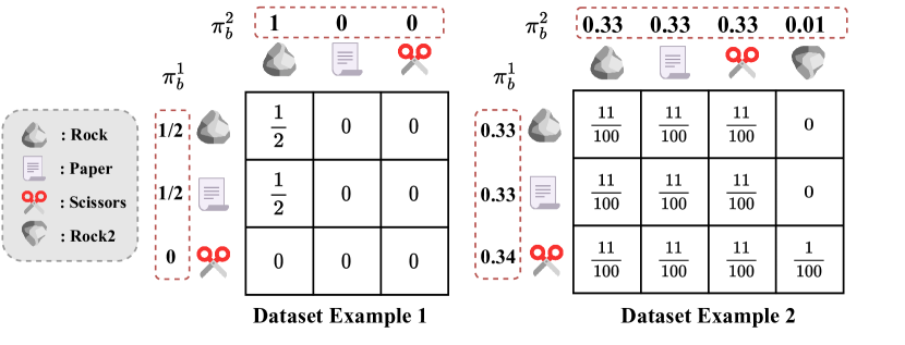
Considering infinite samples, the missing of some $(s,a)$ is caused by $\pi_{b}(s,a)=0$ where $\pi_{b}$ is the behavior strategy to sample the dataset. We show this case in a simple matrix game, Rock-Paper-Scissors(RPS), with the first example of Figure 4. In this case, the covered part of the matrix can be seen as a subgame, where agents can only choose actions from observed ones. The payoff of the subgame is known. A conservative solution for this dataset is to find the Nash equilibrium of the subgame. However, if the lower bound of payoff in this game is known, allowing the selection of out-of-distribution actions may be a more reasonable setting. With the knowledge that payoffs of RPS are in the range of $[-1,1]$, player $1$ consistently selects paper as it yields a payoff of $1$. For player $2$, the only action, rock, in the dataset gets a payoff of $-1$, and choosing OOD actions may be a better selection because the rock is already the worst action. Some offline RL algorithms, such as CQL, give the OOD actions low rewards rather than set hard restrictions on these actions, which enables the learned policy to choose OOD actions. The experimental results in  Sections 5.1 and 5.2 show that restricting the policy space to subgames leads to higher exploitability.

Considering finite samples, even if a state-action pair is covered by a dataset, it may still be a challenge to determine its quality. If we use a random policy as a behavior strategy, the dataset still may not cover the entire state-action space. The second example in Figure 4 shows a case of this. We add a second rock action, Rock2, for player $2$. This new action has the same payoff as the original rock action. In the example dataset, the only sample observed in the dataset is $(\text{Scissors},\text{Rock2})$. In player $2$’s perspective, the Rock2 action gets a payoff of $1$ all the time, so choosing it with a probability of $1$ is the best choice. Nevertheless, the strategy has the highest exploitability in the original game, as player $1$ possesses a best response by selecting scissors, resulting in a payoff of $1$ for player $1$. In Off-FSP, this issue can be mitigated by a proper offline RL algorithm in the LearnBestResponse function. Offline RL algorithm maximizes return while simultaneously ensuring learned policy resembles behavior strategy $\pi_{b}$. In this way, the learned best response does not overfit samples with low sampling probability.

5 Experiments

In this section, we design a series of experiments to show the performance of Off-FSP and investigate the OOD issue in offline competitive games. We first evaluate Off-FSP on toy examples in a matrix game, rock-paper-scissors. We compared Off-FSP against the state-of-the-art offline RL methods for competitive games, including OEF (Li et al., 2022), Behavior Cloning (BC), and other single-agent Offline RL methods, on an imperfect-information poker game, Leduc Hold’em. We also conduct ablation studies on Off-FSP in  Section D.2.

To demonstrate the compatibility of our approach with existing single-agent offline RL algorithms, we combine Off-FSP with three methods: CQL (Kumar et al., 2020), BCQ (Fujimoto et al., 2019b) and CRR (Wang et al., 2020). For variants with CQL, denoted as CQL-$\alpha$, we conduct different hyperparameters $\alpha$ which indicates the penalty level of choosing OOD actions. Higher $\alpha$ means less OOD actions performed by the policy. When $\alpha=0$, there is no penalty, and CQL degrades to DQN. More details about the experiments are provided in Appendix C.

5.1 Rock, Paper, Scissors

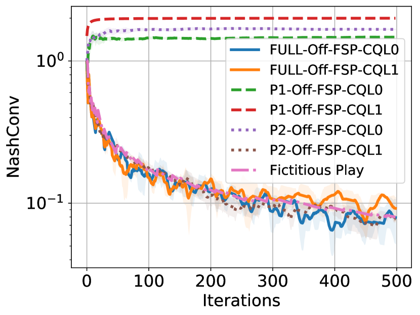
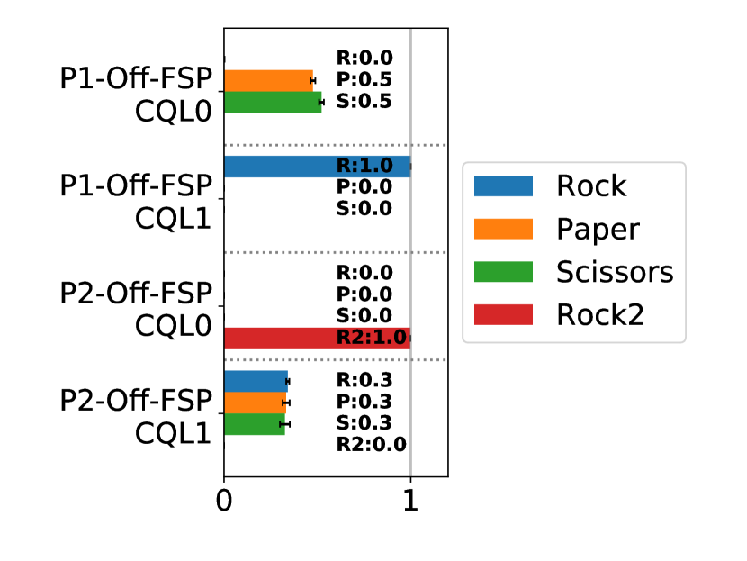
To provide empirical evidence for our statements in Section 4.4 and show the effectiveness of our methods, we first give results on three datasets of rock-paper-scissors. The first dataset, FULL, is randomly sampled from a uniform behavioural strategy, $\pi_{b}=(\frac{1}{3},\frac{1}{3},\frac{1}{3})$, which is a fully covered dataset and an approximation of ideal dataset. P1 and P2 are partially covered datasets described in Figure 4. Figure 5 shows the NashConv within $500$ iterations and the average strategies of player $2$ after the end of training.

In FULL dataset, both CQL-$0$ and CQL-$1$ with Off-FSP are converged to a $\epsilon$-NE with a small gap with online fictitious play. In the partially covered P2 dataset, only CQL with $\alpha>0$ can properly address the OOD issues successfully converges to a $\epsilon$-NE, while CQL-$0$ is misleading by one single sample of Rock2 and selects Rock2 with a probability of $1$. In the P1 scenario, employing CQL with a smaller $\alpha$ value results in a reduced NashConv. This outcome is attributed to the allowance of OOD actions, as elaborated in Section 4.4. The outcomes from experiments P1 and P2 demonstrate the complexities inherent in OOD problems. The findings suggest that neither arbitrary selection nor total exclusion of OOD actions is optimal, emphasizing the need for sophisticated offline algorithms.

Figure 5: Results of RPS. (Left) NashConv. (Right) Player $2$’s Average Strategy.

5.2 Leduc Hold’em

(a) NashConv

(b) OOD ratio

(c) NashConv w/o OOD actions

(d) Payoff

Figure 6: Results of Leduc Hold’em

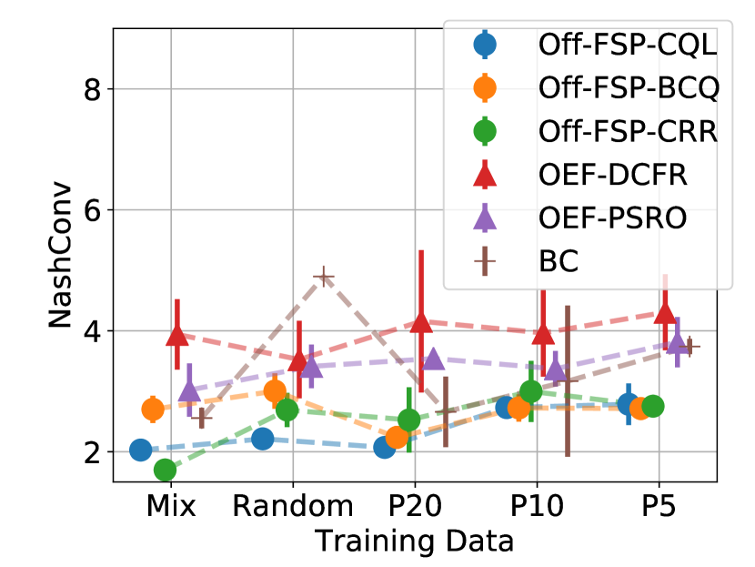
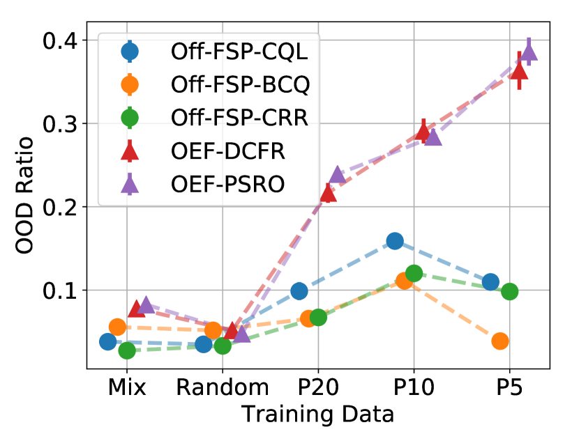
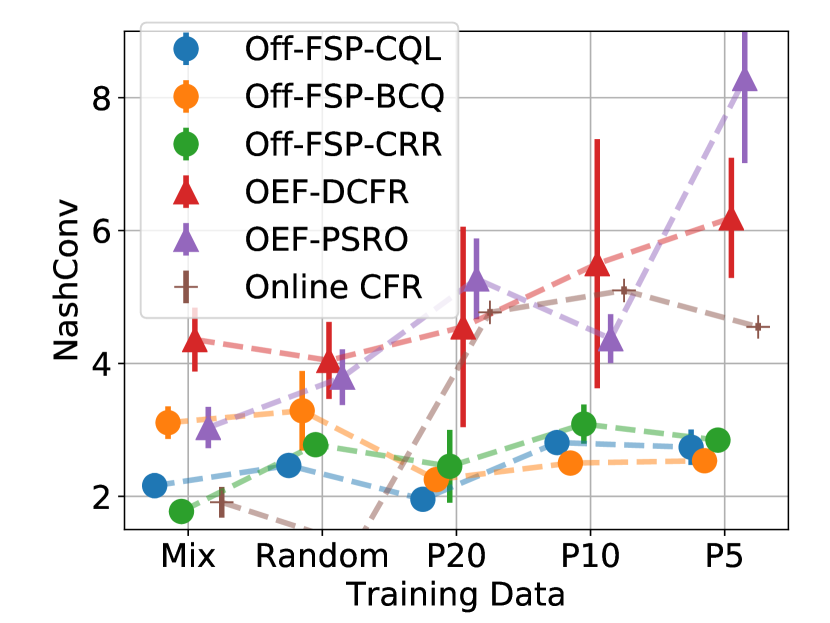
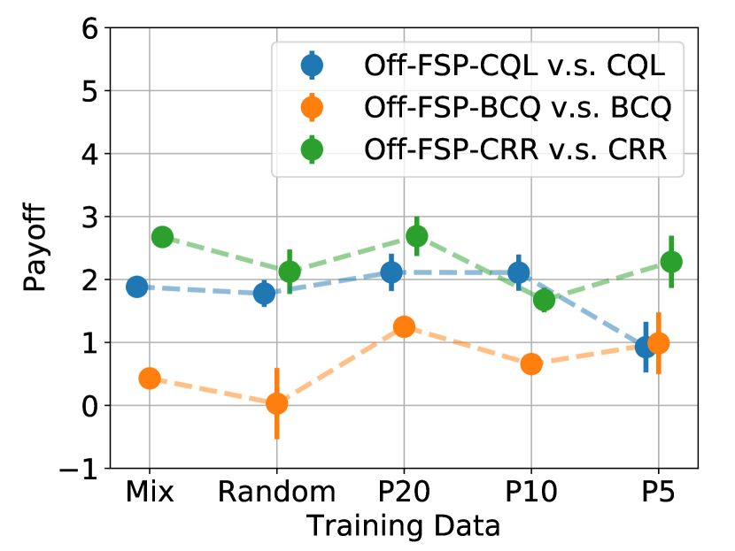
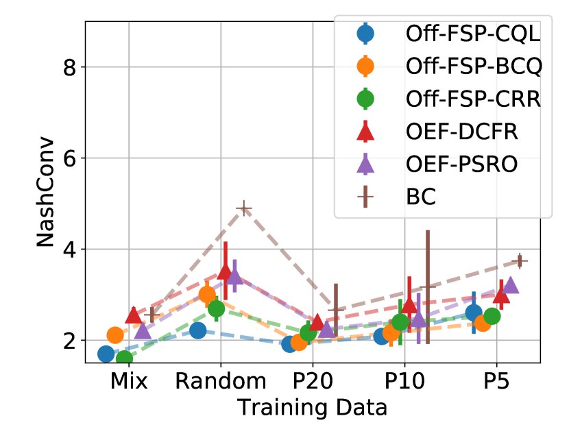
We now show the results compared with existing algorithms for offline competitive games. We collect 5 datasets on Leduc Hold’em with different quality. Mix and Random are nearly fully covered datasets, which are sampled by a random policy and aggregate strategy with expert and random policy. P20, P10, and P5 are partially covered datasets sampled from mixed strategies of $20,10,5$ best responses. These best responses are randomly picked from the training process of online PSRO. The more BR picked for sampling, the more state-action pairs are covered by the datasets. We visualize the ratio of covered state-action pair for all datasets in Appendix D. All these datasets contain $10\,000$ trajectories. Mix and P20 datasets sampled from a high-quality strategy, so we can easily obtain a good strategy by supervised learning their empirical behavioral strategies $\tilde{\pi}_{b}$. This paradigm is also called behavior cloning, which is a popular baseline for offline learning.

We evaluate state-of-the-art offline learning baselines and variants of Off-FSP on all the datasets. Figure 6(a) shows the NashConv of all the algorithms, and all variants of our method outperform other baselines. The result also demonstrates the ability of Off-FSP to robustly integrate with any existing offline RL methods. BC supervised learning the empirical behavioral strategies $\tilde{\pi}_{b}$ of all datasets, which shows Off-FSP can also outperform the sampling strategy. Mix and P20 datasets are both sampled from high-quality strategies, while the Random dataset is sampled from a random strategy. OEF-DCFR and OEF-PSRO are two variants of OEF (Li et al., 2022), which is a model-based offline algorithm for finding NE. OEF mixed its strategy with BC, evaluated it in online games multiple times and used the minimum NashConv as its results. This operation involves interaction with online games, which violates the offline scenario. To fair comparison, we remove the mixing operation in our main experiment. The results with mixing are shown in  Appendix D. OEF operates based on the assumption of full data coverage, so OEF strategies have a high probability of performing OOD actions on partially covered datasets, as shown in Figure 6(b).

To investigate the influence of OOD actions, we restrict all the strategies on the observed state-action pairs and evaluate these restricted strategies. Figure 6(c) demonstrates significant performance degradation in some methods. We also learned an online CFR to find a $\epsilon$-NE on the subgames of different datasets. For partially covered datasets, the $\epsilon$-NE shows large NashConv values. This indicates that directly solving NE in subgames is insufficient for resolving the offline learning problem in competitive games.

In previous works (Mathieu et al., 2023; Qu et al., 2023), directly applying single-agent Offline RL on the fixed dataset is also an attempt to solve offline competitive games. This paradigm is identical to learning best responses to the behavioural strategies $\pi_{b}$. These strategies overfit their opponents and are vulnerable to exploitation. These works only pay attention to strategies with higher returns and do not discuss NE. Therefore, we show the payoff of variants of Off-FSP playing with corresponding single-agent Offline RL algorithms, as Figure 6(d). Our methods show positive payoff to all the single-agent methods.

6 Conclusion

In this paper, we study offline multi-agent reinforcement learning for competitive games and propose Off-SP and Off-FSP to enable single-agent offline RL algorithms to be applied in this scenario. We find that Off-FSP can approximate NE even with partially covered datasets. Extensive experiments show that all variants of Off-FSP significantly outperform state-of-the-art baselines in different datasets of an imperfect-information two-player zero-sum game, Leduc Hold’em.

Impact Statements

This paper presents work whose goal is to advance the field of Machine Learning. There are many potential societal consequences of our work, none which we feel must be specifically highlighted here.

Appendix A Derivation of Theorem

Proof.

Now we derive the weight when changing the opponent to $\pi_{-i}$. Since we do not need to adjust player $i$’s strategy, player $i$’s strategy is still considered as $\tilde{\pi}_{b}^{i}$. In player $i$’s perspective, the reach probability of a tuple $d_{t}=(s^{i}_{t},a^{i}_{t},s^{i}_{t+1})$ is

$$Pr(d_{t}|\pi^{-i})=\Pi_{j=0}^{t}\pi^{i}(s^{i}_{j},a^{i}_{j})\mathcal{T}_{\pi^{-i}}(s^{i}_{j+1}|s^{i}_{j},a^{i}_{j})\cdot\pi^{i}(a^{i}_{t+1}|s^{i}_{t+1}),$$

where $\mathcal{T}_{\pi^{-i}}$ is the transition function under MDP $\mathcal{M}(\pi^{-i})$. So we have:

$$w_{\pi^{-i}}(d_{t}) =\frac{Pr(d_{t}|\pi^{-i})}{Pr(d_{t}|\tilde{\pi}^{-i}_{b})}$$

$$=\frac{\Pi_{j=0}^{t}\tilde{\pi}_{b}^{i}(s^{i}_{j},a^{i}_{j})\mathcal{T}_{\pi^{-i}}(s^{i}_{j+1}|s^{i}_{j},a^{i}_{j})}{\Pi_{j=0}^{t}\tilde{\pi}_{b}^{i}(s^{i}_{j},a^{i}_{j})\mathcal{T}_{\tilde{\pi}_{b}^{-i}}(s^{i}_{j+1}|s^{i}_{j},a^{i}_{j})}\cdot\frac{\tilde{\pi}_{b}^{i}(a^{i}_{t+1}|s^{i}_{t+1})}{\tilde{\pi}_{b}^{i}(a^{i}_{t+1}|s^{i}_{t+1})}$$

$$=\Pi_{j=0}^{t}\frac{\mathcal{T}_{\pi^{-i}}(s^{i}_{j+1}|s^{i}_{j},a^{i}_{j})}{\mathcal{T}_{\tilde{\pi}_{b}^{-i}}(s^{i}_{j+1}|s_{j},a_{j})}$$

Considering $\mathcal{T}_{\pi^{-i}}(s^{i}_{j+1}|s^{i}_{j},a^{i}_{j})$ and $\mathcal{T}_{\tilde{\pi}_{b}^{-i}}(s^{i}_{j+1}|s_{j},a_{j})$, both of these two items are the multiplication of a series of transition probabilities, of which only the probability of opponents’ strategies $\pi^{-i}$ is different. So the above equation can be simplified to:

$$w_{\pi^{-i}}(d_{t}) =\Pi_{j=0}^{t}\frac{{\pi^{-i}}(a_{j}|s_{j})}{{\tilde{\pi}_{b}^{-i}}(a_{j}|s_{j})}$$

$$=\frac{x_{\pi^{-i}}(s_{j}){\pi^{-i}}(a_{j}|s_{j})}{x_{\tilde{\pi}_{b}^{-i}}(s_{j}){\tilde{\pi}_{b}^{-i}}(a_{j}|s_{j})},$$

where $s_{j}=\tau_{<}^{-i}(s_{t+1}^{i})$. ∎

Appendix B Baselines

Behaviour Cloning (BC).

Behaviour Cloning directly learns the probability distribution of actions conditioned on the observation from the dataset, hoping to recover the performance of the behavior policy used to generate the dataset.

Conservative Q-Learning (CQL)

Conservative Q-Learning (Kumar et al., 2020) learns a conservative Q-function such that the expected value of a policy under this Q-function lower-bounds its actual value in order to alleviate overestimation of values induced by the distributional shift between dataset and the learned policy. In practice, we solve such an optimization problem to update our Q-function, where the first term is the penalty for lower-bounding the Q-function, and the second term is the Bellman error. We use CQL based on the QRDQN.

$$\min_{Q}\alpha\mathbb{E}_{\mathbf{s}\sim\mathcal{D}}\left[\log\sum_{\mathbf{a}}\exp(Q(\mathbf{s},\mathbf{a}))-\mathbb{E}_{\mathbf{a}\sim\hat{\pi}_{\beta}(\mathbf{a}\mid\mathbf{s})}[Q(\mathbf{s},\mathbf{a})]\right]+\frac{1}{2}\mathbb{E}_{\mathbf{s},\mathbf{a},\mathbf{s}^{\prime}\sim\mathcal{D}}\left[\left(Q-\hat{\mathcal{B}}^{\pi_{k}}\hat{Q}^{k}\right)^{2}\right]$$ (4)

Critic Regularized Regression (CRR)

Critic Regularized Regression (Wang et al., 2020) handles the problem of offline policy optimization by value-filtered regression. It selectively imitates the dataset by choosing a function $f$ that is monotonically increasing in $Q_{\theta}$.

$$\underset{\pi}{\arg\max}\ \mathbb{E}_{(\mathbf{s},\mathbf{a})\sim\mathcal{D}}\left[f\left(Q_{\theta},\pi,\mathbf{s},\mathbf{a}\right)\log\pi(\mathbf{a}\mid\mathbf{s})\right]$$ (5)

Batch-Constrained deep Q-learning (BCQ)

Batch-Constrained deep Q-learning (Fujimoto et al., 2019b) uses a generative model to learn the distribution of transitions in the dataset, samples several actions from it in the current state, perturbates them and chooses the one with highest Q value. In this way, they tried to minimize the distance of selected actions to the dataset and lead to states similar to those in the dataset. In the experiments, we use a discrete BCQ variant introduced in (Fujimoto et al., 2019a).

Single-Agent Offline RL

In this set of baseline methods, each player independently learns a policy from the dataset using single-agent offline RL algorithms, including CQL, CRR, and BCQ. It’s theoretically equivalent to figuring out the best response to the fixed opponent policy used to collect the dataset. This kind of method is also employed in Qu et al. (2023) and Mathieu et al. (2023).

Offline Equilibrium Finding (OEF)

Offline Equilibrium Finding (Li et al., 2022) is a model-based framework to find the game equilibrium in the offline setting. They directly train a model to describe the game dynamics and apply online equilibrium-finding algorithms like PSRO and DCFR (a deep learning version of CFR) to compute equilibrium. They also combine the behavior cloning policy with the model-based policy for improvement, where they mix these two policies with different weights and evaluate each weight in the online game to find the best combination.

Appendix C Details of experiments

C.1 Datasets

C.1.1 Rock, Paper, Scissors

FULL is randomly sampled from a uniform behavioral strategy, $\pi_{b}=(\frac{1}{3},\frac{1}{3},\frac{1}{3})$, i.e., every player randomly picks each action with the same probability. P1 and P2 are generated according to the exact proportion described in Figure 4, e.g., P1 comprises 500 episodes of Rock to Rock and 500 episodes of Paper to Rock.

Every dataset is composed of 1000 trajectories.

C.1.2 Leduc Hold’em

Random is sampled by uniformly randomly picking action from all legal actions in every decision node.

Mix is sampled from a mixed strategy, which is a 3-to-1 mix of expert and random strategies. The expert strategy is trained by PSRO with 30 iterations and is a mix of 30 deterministic policies according to a specific ratio.

Partial dataset (5-10-20) is sampled by first picking 5, 10, and 20 policies from the 30 components of the expert strategy and then uniformly mixing them to form the sampling strategy.

Every dataset comprises 10000 trajectories except those used in ablation study about the dataset size.

C.2 Variants of Off-FSP

Off-FSP-CQl, Off-FSP-CRR, and Off-FSP-CQL are different variants of our methods that integrate with different single-agent offline RL methods in the function of LearnBestResponse. We then introduce details about these Offline RL methods.

In CQL, we use a QRDQN as the base algorithm and a simple MLP as the Q network. Hence, the network’s input is the observation vector, and the output has a dimension of the number of quantiles times the number of actions. The hidden layer of MLP contains the same number of neurons. We use ReLU as the activation function between every linear layer.

In CRR, the actor and critic networks have the same structure, first a shared feature network and then a MLP head. The shared feature network is a MLP with two layers, and the size of the second layer is the number of actions. All activation functions are ReLU. CQL penalty term is also added to the CRR objective function for better performance.

In BCQ, the policy network and the imitation network have the same structure, which is also first a shared feature network and then an MLP head, exactly the same as CRR.

C.3 Hyperparameters

In OEF, all settings are the same as Li et al. (2022).

In RPS, we use Adam optimizer with a learning rate of 0.005 and betas (0.9, 0.999), and the network has only one layer, and the number of quantiles in QRDQN is 100. The target network is not used. In each iteration, the network is trained five epochs and is updated 100 times each epoch with a batch size of 1000.

In Leduc, the hyperparamters are shown in Table 1. All networks are optimized by Adam Optimizer (Kingma & Ba, 2017). The hidden layer number of CRR and BCQ describes the whole network, including the feature network and MLP head. The target network is used.

Table 1: Hyperparameters used in Leduc

Hyperparameter	CQL	CRR	BCQ
Hidden layer number	4	5	6
Hidden layer size	256	128	256
Learning rate	0.0001	0.0001	0.0001
Adam $(\beta_{1},\beta_{2})$	(0.9, 0.999)	(0.9, 0.999)	(0.9, 0.999)
Training steps per iteration $M$	1 000	1 000	1 000
Target Network update frequency	100	100	100
Batch size	1024	1024	1024
QRDQN number of quantiles	100
CQL $\alpha$	0.1	0.1
BCQ unlikely action threshold			0.1
BCQ imitation logits penalty			0.01
CRR improve mode		Exponential
CRR $\beta$		1
CRR ratio bound		20

Appendix D Supplement Results

D.1 Analysis of Datasets

Figure 7: State-Action Cover Ratio

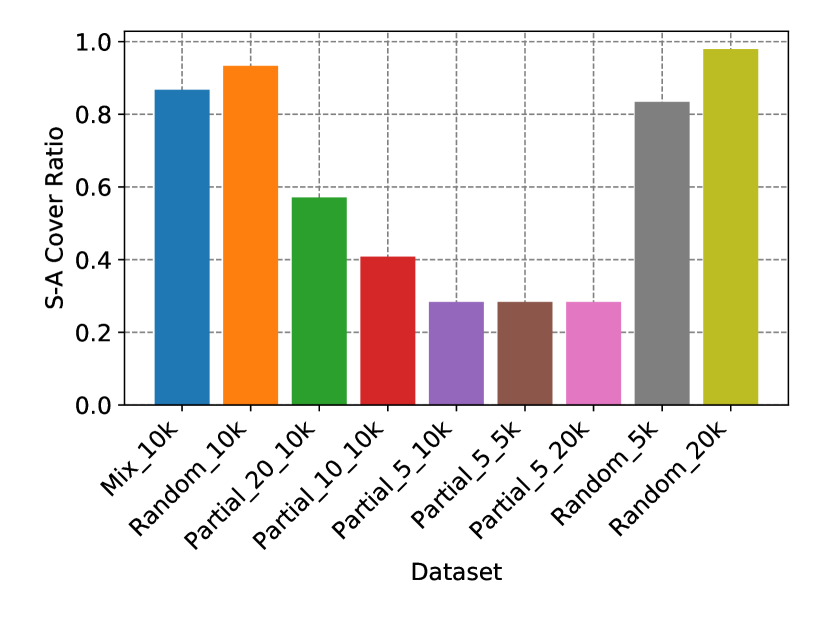
We visualize the state-action cover ratio of different datasets in Figure 7

D.2 Ablations

(a) Value of $\alpha$

(b) Size of Data

Figure 8: Results of ablations.

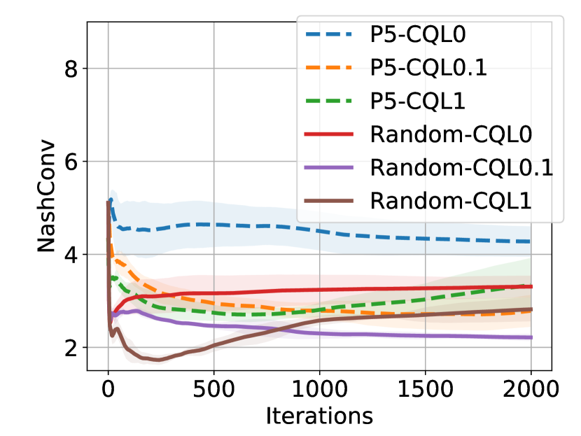
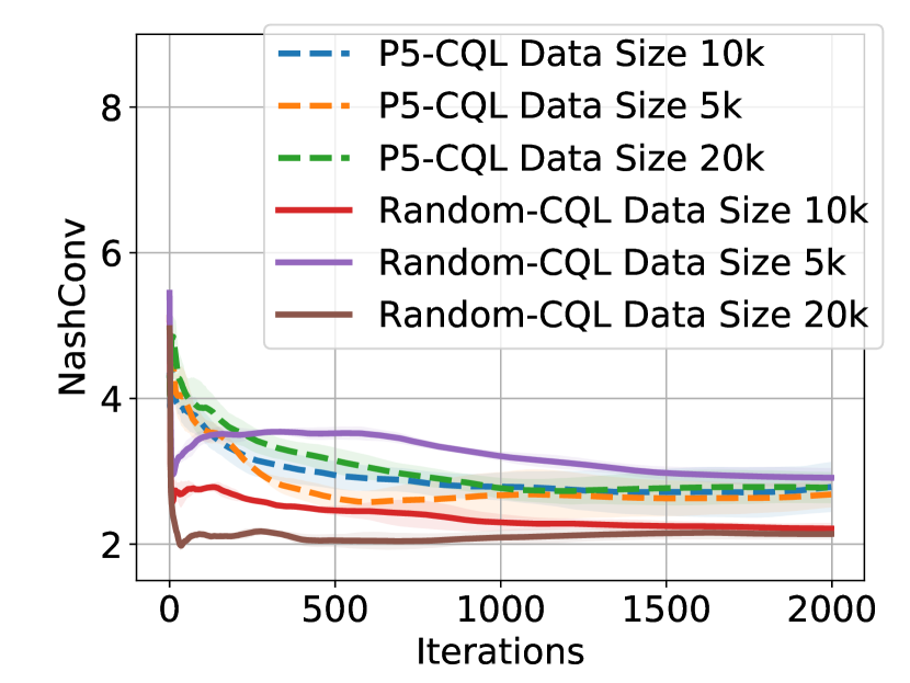
We evaluate two factors that affect the performance of Off-FSP, the degree of restriction on OOD actions and the size of datasets, on dataset Random and P5. Figure 8(a) shows NashConv of training Off-FSP-CQL with $\alpha$ of $(0,0.1,1)$. Excessive restrictions with $\alpha=1$ on OOD actions harm the results. If the OOD action is not restricted at all, the algorithm will completely fail in seriously incomplete P5 dataset, which is consistent with the results on FULL and P1 datasets of RPS.  Figure 8(b) shows NashConv of training Off-FSP-CQL on datasets with sizes of $5000,10\,000,\text{and}~{}20\,000$. For datasets that cover more state-action pairs, e.g., Random dataset, increasing the amount of data has a more obvious effect on the performance.

D.3 Learning Curves of Off-FSP

OEF evaluates strategies’ performance by allowing strategies to mix with BC by different weights. However, the results are decided by the best-mixed strategies. This is equivalent to allowing strategies to be interactively evaluated online, which is contrary to the setting of offline scenarios. And we cannot tell whether this result is caused by the original strategy or BC. We still provide the final results under this evaluation method in Figure 9, and our method still outperforms OEF.

Figure 9: NashConv with evaluation method in OEF

References

- Bowling et al. (2015) Bowling, M., Burch, N., Johanson, M., and Tammelin, O. Heads-up limit hold’em poker is solved. Science, 347(6218):145–149, 2015.
- Brown (1951) Brown, G. W. Iterative solution of games by fictitious play. Act. Anal. Prod Allocation, 13(1):374, 1951.
- Brown & Sandholm (2018) Brown, N. and Sandholm, T. Superhuman ai for heads-up no-limit poker: Libratus beats top professionals. Science, 359(6374):418–424, 2018.
- Brown & Sandholm (2019) Brown, N. and Sandholm, T. Superhuman ai for multiplayer poker. Science, 365(6456):885–890, 2019.
- Cui & Du (2022a) Cui, Q. and Du, S. S. When are offline two-player zero-sum markov games solvable? Advances in Neural Information Processing Systems, 35:25779–25791, 2022a.
- Cui & Du (2022b) Cui, Q. and Du, S. S. Provably efficient offline multi-agent reinforcement learning via strategy-wise bonus. Advances in Neural Information Processing Systems, 35:11739–11751, 2022b.
- Fang et al. (2016) Fang, F., Nguyen, T., Pickles, R., Lam, W., Clements, G., An, B., Singh, A., Tambe, M., and Lemieux, A. Deploying paws: Field optimization of the protection assistant for wildlife security. In Proceedings of the AAAI Conference on Artificial Intelligence, volume 30, pp. 3966–3973, 2016.
- Fujimoto et al. (2019a) Fujimoto, S., Conti, E., Ghavamzadeh, M., and Pineau, J. Benchmarking batch deep reinforcement learning algorithms, 2019a.
- Fujimoto et al. (2019b) Fujimoto, S., Meger, D., and Precup, D. Off-policy deep reinforcement learning without exploration. In International conference on machine learning, pp. 2052–2062. PMLR, 2019b.
- Gerstgrasser et al. (2021) Gerstgrasser, M., Trivedi, R., and Parkes, D. C. Crowdplay: Crowdsourcing human demonstrations for offline learning. In International Conference on Learning Representations, 2021.
- Greenwald et al. (2013) Greenwald, A., Li, J., Sodomka, E., and Littman, M. Solving for best responses in extensive-form games using reinforcement learning methods. RLDM 2013, pp. 116, 2013.
- Heinrich et al. (2015) Heinrich, J., Lanctot, M., and Silver, D. Fictitious self-play in extensive-form games. In International conference on machine learning, pp. 805–813. PMLR, 2015.
- Hong et al. (2023) Hong, Z.-W., Kumar, A., Karnik, S., Bhandwaldar, A., Srivastava, A., Pajarinen, J., Laroche, R., Gupta, A., and Agrawal, P. Beyond uniform sampling: Offline reinforcement learning with imbalanced datasets. arXiv preprint arXiv:2310.04413, 2023.
- Kingma & Ba (2017) Kingma, D. P. and Ba, J. Adam: A method for stochastic optimization, 2017.
- Kumar et al. (2020) Kumar, A., Zhou, A., Tucker, G., and Levine, S. Conservative q-learning for offline reinforcement learning. Advances in Neural Information Processing Systems, 33:1179–1191, 2020.
- Kurach et al. (2020) Kurach, K., Raichuk, A., Stańczyk, P., Zając, M., Bachem, O., Espeholt, L., Riquelme, C., Vincent, D., Michalski, M., Bousquet, O., et al. Google research football: A novel reinforcement learning environment. In Proceedings of the AAAI conference on artificial intelligence, volume 34, pp. 4501–4510, 2020.
- Lanctot et al. (2017) Lanctot, M., Zambaldi, V., Gruslys, A., Lazaridou, A., Tuyls, K., Pérolat, J., Silver, D., and Graepel, T. A unified game-theoretic approach to multiagent reinforcement learning. Advances in neural information processing systems, 30, 2017.
- Leslie & Collins (2006) Leslie, D. S. and Collins, E. J. Generalised weakened fictitious play. Games and Economic Behavior, 56(2):285–298, 2006.
- Li et al. (2022) Li, S., Wang, X., Zhang, Y., Cerny, J., Li, P., Chan, H., and An, B. Offline equilibrium finding. arXiv preprint arXiv:2207.05285, 2022.
- Mathieu et al. (2023) Mathieu, M., Ozair, S., Srinivasan, S., Gulcehre, C., Zhang, S., Jiang, R., Paine, T. L., Powell, R., Żołna, K., Schrittwieser, J., et al. Alphastar unplugged: Large-scale offline reinforcement learning. arXiv preprint arXiv:2308.03526, 2023.
- Munos et al. (2016) Munos, R., Stepleton, T., Harutyunyan, A., and Bellemare, M. Safe and efficient off-policy reinforcement learning. Advances in neural information processing systems, 29, 2016.
- Nachum et al. (2019) Nachum, O., Chow, Y., Dai, B., and Li, L. Dualdice: Behavior-agnostic estimation of discounted stationary distribution corrections. Advances in neural information processing systems, 32, 2019.
- Perolat et al. (2022) Perolat, J., De Vylder, B., Hennes, D., Tarassov, E., Strub, F., de Boer, V., Muller, P., Connor, J. T., Burch, N., Anthony, T., et al. Mastering the game of stratego with model-free multiagent reinforcement learning. Science, 378(6623):990–996, 2022.
- Qu et al. (2023) Qu, Y., Wang, B., Shao, J., Jiang, Y., Chen, C., Ye, Z., Liu, L., Feng, Y. J., Lai, L., Qin, H., et al. Hokoff: Real game dataset from honor of kings and its offline reinforcement learning benchmarks. In Thirty-seventh Conference on Neural Information Processing Systems Datasets and Benchmarks Track, 2023.
- Silver & Veness (2010) Silver, D. and Veness, J. Monte-carlo planning in large pomdps. Advances in neural information processing systems, 23, 2010.
- Silver et al. (2017) Silver, D., Hubert, T., Schrittwieser, J., Antonoglou, I., Lai, M., Guez, A., Lanctot, M., Sifre, L., Kumaran, D., Graepel, T., et al. Mastering chess and shogi by self-play with a general reinforcement learning algorithm. arXiv preprint arXiv:1712.01815, 2017.
- Timbers et al. (2022) Timbers, F., Bard, N., Lockhart, E., Lanctot, M., Schmid, M., Burch, N., Schrittwieser, J., Hubert, T., and Bowling, M. Approximate exploitability: learning a best response. In Proceedings of the International Joint Conference on Artificial Intelligence (IJCAI), pp. 3487–3493, 2022.
- Tseng et al. (2022) Tseng, W.-C., Wang, T.-H. J., Lin, Y.-C., and Isola, P. Offline multi-agent reinforcement learning with knowledge distillation. Advances in Neural Information Processing Systems, 35:226–237, 2022.
- Vinyals et al. (2019) Vinyals, O., Babuschkin, I., Czarnecki, W. M., Mathieu, M., Dudzik, A., Chung, J., Choi, D. H., Powell, R., Ewalds, T., Georgiev, P., et al. Grandmaster level in starcraft ii using multi-agent reinforcement learning. Nature, 575(7782):350–354, 2019.
- Von Stengel (1996) Von Stengel, B. Efficient computation of behavior strategies. Games and Economic Behavior, 14(2):220–246, 1996.
- Wang et al. (2020) Wang, Z., Novikov, A., Zolna, K., Merel, J. S., Springenberg, J. T., Reed, S. E., Shahriari, B., Siegel, N., Gulcehre, C., Heess, N., et al. Critic regularized regression. Advances in Neural Information Processing Systems, 33:7768–7778, 2020.
- Wei et al. (2022) Wei, H., Chen, J., Ji, X., Qin, H., Deng, M., Li, S., Wang, L., Zhang, W., Yu, Y., Linc, L., et al. Honor of kings arena: an environment for generalization in competitive reinforcement learning. Advances in Neural Information Processing Systems, 35:11881–11892, 2022.
- Yan et al. (2022) Yan, Y., Li, G., Chen, Y., and Fan, J. Model-based reinforcement learning is minimax-optimal for offline zero-sum markov games. arXiv preprint arXiv:2206.04044, 2022.
- Yang et al. (2022) Yang, G., Liu, M., Hong, W., Zhang, W., Fang, F., Zeng, G., and Lin, Y. Perfectdou: Dominating doudizhu with perfect information distillation. Advances in Neural Information Processing Systems, 35:34954–34965, 2022.
- Yang et al. (2020) Yang, R., Chen, J., and Narasimhan, K. Improving dialog systems for negotiation with personality modeling. arXiv preprint arXiv:2010.09954, 2020.
- Yang et al. (2021) Yang, Y., Ma, X., Li, C., Zheng, Z., Zhang, Q., Huang, G., Yang, J., and Zhao, Q. Believe what you see: Implicit constraint approach for offline multi-agent reinforcement learning. Advances in Neural Information Processing Systems, 34:10299–10312, 2021.
- Ye et al. (2015) Ye, D., Zhang, M., and Yang, Y. A multi-agent framework for packet routing in wireless sensor networks. sensors, 15(5):10026–10047, 2015.
- Ye et al. (2020) Ye, D., Chen, G., Zhang, W., Chen, S., Yuan, B., Liu, B., Chen, J., Liu, Z., Qiu, F., Yu, H., et al. Towards playing full moba games with deep reinforcement learning. Advances in Neural Information Processing Systems, 33:621–632, 2020.
- Yu et al. (2023) Yu, C., Yang, X., Gao, J., Chen, J., Li, Y., Liu, J., Xiang, Y., Huang, R., Yang, H., Wu, Y., et al. Asynchronous multi-agent reinforcement learning for efficient real-time multi-robot cooperative exploration. arXiv preprint arXiv:2301.03398, 2023.
- Yun et al. (2022) Yun, W. J., Park, S., Kim, J., Shin, M., Jung, S., Mohaisen, D. A., and Kim, J.-H. Cooperative multiagent deep reinforcement learning for reliable surveillance via autonomous multi-uav control. IEEE Transactions on Industrial Informatics, 18(10):7086–7096, 2022.
- Zhong et al. (2022) Zhong, H., Xiong, W., Tan, J., Wang, L., Zhang, T., Wang, Z., and Yang, Z. Pessimistic minimax value iteration: Provably efficient equilibrium learning from offline datasets. In International Conference on Machine Learning, pp. 27117–27142. PMLR, 2022.