Towards a Theoretical Understanding of Two-Stage Recommender Systems

Abstract

Production-grade recommender systems rely heavily on a large-scale corpus used by online media services, including Netflix, Pinterest, and Amazon. These systems enrich recommendations by learning users’ and items’ embeddings projected in a low-dimensional space with two-stage models (two deep neural networks), which facilitate their embedding constructs to predict users’ feedback associated with items. Despite its popularity for recommendations, its theoretical behaviors remain comprehensively unexplored. We study the asymptotic behaviors of the two-stage recommender that entail a strong convergence to the optimal recommender system. We establish certain theoretical properties and statistical assurance of the two-stage recommender. In addition to asymptotic behaviors, we demonstrate that the two-stage recommender system attains faster convergence by relying on the intrinsic dimensions of the input features. Finally, we show numerically that the two-stage recommender enables encapsulating the impacts of items’ and users’ attributes on ratings, resulting in better performance compared to existing methods conducted using synthetic and real-world data experiments.

1 Introduction

Recommender systems are pivotal to enabling contents consumption for users’ across various online media platforms, affecting what media items we interact, or navigate through in order to incentivize exploration. Moreover, recommender system has garnered significant attention over the past decades and have become massively popular, especially in machine learning community due to its widespread use in precision marketing and E-commerce, such as news feeding (Li et al., 2016), movie recommendation (Miller et al., 2003), online shopping (Romadhony et al., 2013), and restaurant recommendation (Vargas-Govea et al., 2011). Content-based recommender systems (Lang, 1995; Pazzani & Billsus, 2007) pertain preprocessing techniques to renovate unstructured the contents of item and the user profiles into numerical vectors. These vectors are then employed as inputs for classical machine learning algorithms, such as decision trees (Middleton et al., 2004), kNN (Subramaniyaswamy & Logesh, 2017), and SVM (Oku et al., 2006; Fortuna et al., 2010). Collaborative filtering approaches (Hofmann & Puzicha, 1999; Schafer et al., 2007) predict a user’s ratings based on the ratings of similar users or items, and employ techniques such as singular value decomposition (SVD) (Mazumder et al., 2010), restricted Boltzmann machines (RBM) (Salakhutdinov et al., 2007), probabilistic latent semantic analysis (Hofmann, 2004), and nearest neighbour methods (Koren et al., 2009). Hybrid recommender systems (Bostandjiev et al., 2012) aim to integrate collaborative filtering and content-based filtering techniques, exemplified by the unified Boltzmann machines (Gunawardana & Meek, 2009) and partial latent vector model (Kouki et al., 2015). A unified Boltzmann machine introduces a means of encoding both content and collaborative information as features for the purpose of rating prediction. HyPER (Kouki et al., 2015) presented a statistical relational learning framework capable of consolidating multi-level information sources, including user-user and item-item similarity measures, content, and social information. It uses probabilistic soft logic to make predictions, and can automatically learn to balance different information signals. The utilization of deep neural networks in recommender systems has gained widespread adoption in recent years, with various applications demonstrating significant success. Among the neural network models commonly used for recommendation systems, the two-tower model (Yi et al., 2019) has gained significant traction. This model employs two deep neural networks, known as towers, which function as encoders to embed high-dimensional features of both users and items into a low-dimensional space. The two-tower model offers a significant advantage in its ability to address the well-established cold-start problem by integrating features of both users and items to generate precise recommendations for new users or items. Despite its widespread use in applications, such as book recommendation (Lu et al., 2022), application recommendation (Yang et al., 2020), and video recommendation (Yi et al., 2019), the theoretical underpinnings of the two-tower model remain largely underdeveloped in literature.

Contributions:

The primary contribution of our work involves establishing asymptotic characteristics of the two-tower recommender system concerning its robust convergence towards an optimal recommender system. We conduct a thorough analysis of the approximation and estimation errors of the two-tower recommender system, assuming the smoothness of each embedding dimension of user or item features is a continuous function of the corresponding input characteristics. The results indicate that the robust convergence of the two-tower recommender system is closely associated with the smoothness of the optimal recommender system, as well as the inherent dimensionality of the user and item features. Moreover, it is observed that the rate of convergence of the two-tower model increases as the smoothness of the true model improves or the maximum intrinsic dimensions of user and item features decrease. In particular, as the underlying smoothness approaches infinity, the convergence rate of the two-tower model is bounded by $O_{p}\left(\left|\Omega\right|^{-1}(\log\left|\Omega\right|)^{2}\right)$, where $\Omega$ represents the set of observed ratings, and $\left|\cdot\right|$ represents the cardinality of a set. This convergence rate is faster than the majority of the existing theoretical results outlined in (Zhu et al., 2016). More importantly, the established statistical guarantee for the two-tower model serves as a strong theoretical justification for its successful application in a wide range of scenarios.

2 Prior Work

Two-Stage Recommender Systems: The industry has widely embraced two-stage recommender systems, characterized by a candidate generation phase followed by a ranking process. Prominent examples of such systems can be found in platforms like LinkedIn (Borisyuk et al., 2016), YouTube (Yi et al., 2019; Zhao et al., 2019), and Pinterest (Eksombatchai et al., 2018). Such two-stage architecture enables the real-time recommendation of highly personalized items from a vast item space. Most of such methods are dedicated to enhancing both the efficiency (Yi et al., 2019; Kang & McAuley, 2019) and recommendation quality (Chen et al., 2019a; Zhao et al., 2019) within the framework of this general approach, indicating a sustained commitment to refining and optimizing these systems. An instance of two-stage recommendations is two-tower architecture (Yi et al., 2019), which represents a comprehensive framework comprising a query encoder and a candidate encoder. This architectural design has gained substantial traction in the realm of large-scale recommendation systems, as evidenced by its adoption in notable studies (Cen et al., 2020; Yang et al., 2020; Lu et al., 2022). Furthermore, it has emerged as a prominent approach in content-aware scenarios (Ge et al., 2020). Notably, the application of two-tower models within recommendation systems typically involves significantly larger corpora compared to their usage in language retrieval tasks, thereby presenting the challenge of training efficiency. Our work primarily centers on the quantification and behavioral aspects of two-tower recommendation, with particular emphasis placed on optimizing the overall recommendation performance by explicitly considering the multi-level covariates information.
Hybrid Recommendation Systems: Ascertaining a singular model capable of achieving optimal performance across all scenarios is unattainable (Luo et al., 2020). Consequently, the simultaneous deployment of two or more recommenders is widely embraced to capitalize on their respective strengths (Burke, 2002). Considering that collaborative methods excel when ample data is available, while content-based recommendation exhibits superiority in cold-start situations, prior discussions have centered on a hybrid framework that combines content-based filtering with collaborative filtering. This integration facilitates a system that accommodates both new and existing users (Geetha et al., 2018). Early integration techniques typically involve computing a linear combination of individual output scores to amalgamate the outcomes produced by diverse recommenders (Ekstrand & Riedl, 2012).

3 Preliminaries

Let Supp($\mu$) be the spectrum (or support) of a given probability measure $\mu$. Given a function $g$ defined as $g:\mathbb{R}^{D}\rightarrow\mathbb{R}$ with its $L^{2}(\mu)$-norm and $L^{\infty}(\mu)$-norm with respect to a non-negative measure ($\mu$) are $\left\|g\right\|_{L^{2}(\mu)}=\sqrt{\int_{x}g^{2}(x)d\mu(x)}$ and $\left\|g\right\|_{L^{\infty}(\mu)}=\sup_{x\in\text{Supp}(\mu)}g(x)$, respectively. We denote the $l_{2}$-norm of a vector $x$ as $\left\|x\right\|_{2}$ which is equal to $\sqrt{\sum^{p}_{i=1}x^{2}_{i}}$. Given a set $S$, we establish the definition of $\mathcal{N}(\epsilon,S,\left\|\cdot\right\|)$ as the least number of $\epsilon$-balls required to encompass $S$ utilizing a generic metric $\left\|\cdot\right\|$. We can define an $L$-layer neural network which can be viewed as a composition of individual functions formulated as $f(x,\Theta)=h_{L}\circ h_{L-1}\circ\ldots\circ h_{1}(x)$, where the entirety of the parameters is represented by $\Theta=((A_{1},B_{1}),\ldots,(A_{L},b_{L}))$, $h_{l}(x)=\sigma(A_{l}x+b_{l})$ designates the $l$-th layer, and $\circ$ refers to function composition. The key components of each layer are $A_{l}\in\mathbb{R}^{p_{l}\times p_{l-1}}$ refers to the weight matrix, and $b_{l}\in\mathbb{R}^{p_{l}}$ refers to the bias term. The number of neurons in the $l$-th layer is represented by $p_{l}$, and $\sigma(\cdot)$ denotes an activation function that acts component-wise. Common examples of activation functions include the sigmoid function $\sigma(x)=1/(1+\exp(-x))$ and the ReLU function $\sigma(x)=\max(x,0)$. In order to simplify notation, the expression $f(x,\Theta)$ will be represented as $f(x)$ where possible. To describe the architecture of the neural network represented by $f$, we designate the number of layers as $U(f)$, the parameter scale is defined as the maximum value of the infinity norm of the bias vector $b_{l}$ and the vectorized weight matrix $A_{l}$, taken over all layers $l$ in $f$. It is represented by $D(f)=\max_{l=1,\ldots,U(f)}\max\left\{\left\|b_{l}\right\|_{\infty},\left\|\text{vec}(A_{l})\right\|_{\infty}\right\}$ and the number of effective parameters as $Z(f)=\sum_{l=1}^{U(f)}(\left|b_{l}\right|_{0}+\left|\text{vec}(A_{l})\right|_{0})$, where $\text{vec}(\cdot)$ is a function that converts a matrix into a vector. Now, we leverage the concept of Hölder space, which is a space of functions that are defined on a given domain and satisfy certain conditions related to their smoothness and regularity (Chen et al., 2019b). Specifically, we can define a function space of Hölder continuous functions and use it to approximate the unknown user-item preference function (Liu et al., 2021). The degree of smoothness or regularity of the function can be controlled by choosing an appropriate value of the Hölder exponent. Assuming a degree of smoothness $\beta\geq 0$, the Hölder space can be defined as follows $\mathcal{H}(\beta,\left[0,1\right]^{D})=\{f\in C^{\left\lfloor\beta\right\rfloor}(\left[0,1\right]^{D})\mid\left\|f\right\|_{\mathcal{H}(\beta,\left[0,1\right]^{D})}<\infty\}$, here, the set $C^{\left\lfloor\beta\right\rfloor}(\left[0,1\right]^{D})$ comprises all functions that have ${\left\lfloor\beta\right\rfloor}$ times differentiable and continuous derivatives on the domain $\left[0,1\right]^{D}$, where $\left\lfloor\cdot\right\rfloor$ represents the floor function. The Hölder norm is described as follows,

$$\left\|f\right\|_{\mathcal{H}(\beta,\left[0,1\right]^{D})}=\max_{\alpha:\left\|\alpha\right\|_{1}<\beta}\sup_{x\in\left[0,1\right]^{D}}\left|\partial^{\alpha}f(x)\right|+$$

$$\max_{\alpha:\left\|\alpha\right\|_{1}=\left\lfloor\beta\right\rfloor}\sup_{x,x^{{}^{\prime}}\in\left[0,1\right]^{D},x\neq x^{{}^{\prime}}}\frac{\left|\partial^{\alpha}f(x)-\partial^{\alpha}f(x^{{}^{\prime}})\right|}{\left\|x-x^{{}^{\prime}}\right\|^{\beta-\left\lfloor\beta\right\rfloor}_{\infty}}$$

where the Hölder exponent $\alpha_{i}\geq 0$ is an integer with $\alpha=(\alpha_{1},\ldots,\alpha_{D})$, and $\partial^{\alpha}f=\partial^{\alpha_{1}}_{1},\ldots,\partial^{\alpha_{D}}_{D}$. Additionally, we generalize the Hölder space $\mathcal{H}(\beta,\left[0,1\right]^{D},M)=\left\{f\in\mathcal{H}(\beta,\left[0,1\right]^{D})\mid\left\|f\right\|_{\mathcal{H}(\beta,\left[0,1\right]^{D})}\leq M\right\}$ to be considered as a closed ball with radius $M$, and so $\mathcal{H}^{p}(\beta,\left[0,1\right]^{D},M)=\mathcal{H}(\beta,\left[0,1\right]^{D},M)\times\mathcal{H}(\beta,\left[0,1\right]^{D},M)\times\ldots\times\mathcal{H}(\beta,\left[0,1\right]^{D},M)$.

4 Two-Stage Recommender System

Our focus in this work is on a specific recommender system approach, namely the two-tower model (Yi et al., 2019), which is a neural network architecture that is often used for two-stage recommendation. The two towers of the model are responsible for the candidate retrieval and ranking stages, respectively. Two-tower models are capable of learning complex relationships between users and items, and it is able to scale to large datasets. In numerous recommender systems, covariates are unstructured and high-dimensional, and may include information such as user profiles and textual item descriptions. There is a prevailing belief that such information can often be represented in a low-dimensional intrinsic form, and can be seamlessly incorporated into the feature engineering phase of a deep learning model. For a standard recommender system with user covariates denoted as $x_{u}\in\mathbb{R}^{D_{u}}$ and item covariates as $\tilde{x}_{i}\in\mathbb{R}^{D_{i}}$, the two-tower model is formulated as in given Equation 1 and a schematic overview in Figure 1. The two deep neural networks are described as $f:\mathbb{R}^{D_{u}}\rightarrow\mathbb{R}^{p}$ and $\tilde{f}:\mathbb{R}^{D_{i}}\rightarrow\mathbb{R}^{p}$ delineating $x_{u}$ and $\tilde{x}_{i}$ into the same $p$-dimensional embedding space. The two-tower model follows recommendation approach to be based on the dot product between the feature vectors extracted from the two towers, $f(x_{u})$ and $\tilde{f}(\tilde{x}_{i})$. The cost function for optimizing the two-tower model can be structured as per Equation 1.

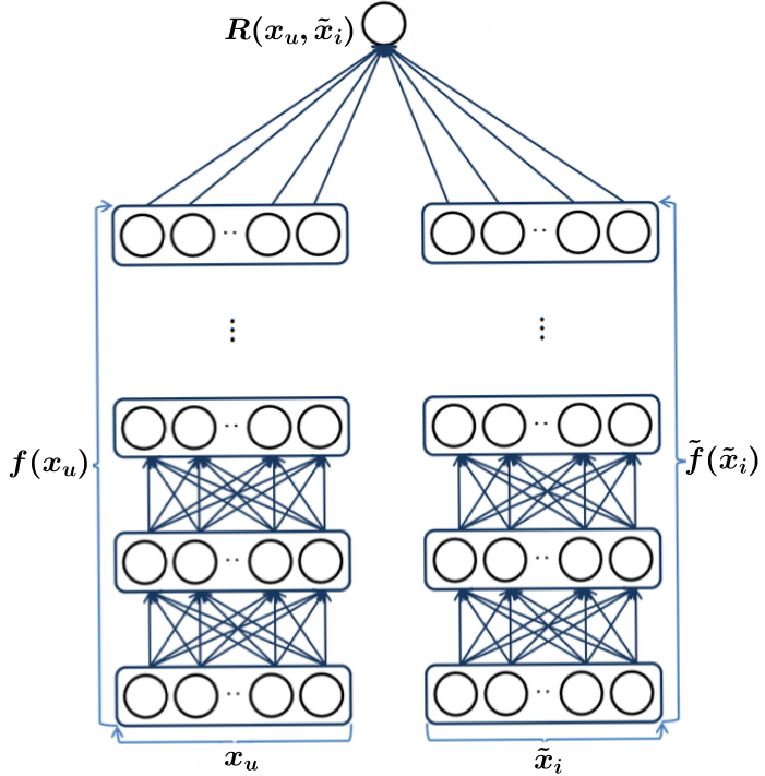
Figure 1: An illustration of the two-tower recommender system.

$$R(x_{u},\tilde{x}_{i})=\langle f(x_{u}),\tilde{f}(\tilde{x}_{i})\rangle$$ (1)

$$\min_{f,\tilde{f}}\frac{1}{\left|\Omega\right|}\sum_{(u,i)\in\Omega}(k_{ui}-\langle f(x_{u}),\tilde{f}(\tilde{x}_{i})\rangle)^{2}$$

$$+\lambda\left\{J(f)+J(\tilde{f})\right\}$$ (2)

This given equation represents the cost function of the two-tower model, where $J(\cdot)$ can be the penalty term of $L_{1}$-norm or $L_{2}$-norm for avoiding overfitting in the deep neural network. The optimization problem presented in Equation 1 can be efficiently solved using an established open-source neural network library such as PyTorch (Paszke et al., 2019). One commonly used approach is to utilize SGD to simultaneously update the parameters of $f(x_{u})$ and $\tilde{f}(\tilde{x}_{i})$, allowing for parallel computation.

$$A^{t+1}_{ljk}=A^{t}_{ljk}+\frac{\alpha}{\left|\mathcal{M}\right|}\sum_{(u,i)\in\mathcal{M}}(k_{ui}-\langle f(x_{u}),\tilde{f}(\tilde{x}_{i})\rangle)$$

$$\langle\frac{d}{dA_{ljk}}f(x_{u}),\tilde{f}(\tilde{x}_{i})\rangle-\alpha\lambda\frac{dJ(f)}{dA_{ljk}},\tilde{A}^{t+1}_{ljk}=$$

$$\tilde{A}^{t}_{ljk}+\frac{\alpha}{\left|\mathcal{M}\right|}\sum_{(u,i)\in\mathcal{M}}(k_{ui}-\langle f(x_{u}),\tilde{f}(\tilde{x}_{i})\rangle)\langle f(x_{u}),$$

$$\frac{d}{d\tilde{A}_{ljk}}\tilde{f}(\tilde{x}_{i})\rangle-\alpha\lambda\frac{dJ(\tilde{f})}{d\tilde{A}_{ljk}},b^{t+1}_{lj}=b^{t}_{lj}+\frac{\alpha}{\left|\mathcal{M}\right|}\sum_{(u,i)\in\mathcal{M}}$$

$$(k_{ui}-\langle f(x_{u}),\tilde{f}(\tilde{x}_{i})\rangle)\langle f(x_{u}),\frac{d}{db_{lj}}\tilde{f}(\tilde{x}_{i})\rangle,\tilde{b}^{t+1}_{lj}=\tilde{b}^{t}_{lj}+$$

$$\frac{\alpha}{\left|\mathcal{M}\right|}\sum_{(u,i)\in\mathcal{M}}(k_{ui}-\langle f(x_{u}),\tilde{f}(\tilde{x}_{i})\rangle)\langle f(x_{u}),\frac{d\tilde{f}}{d\tilde{b}_{lj}}(\tilde{x}_{i})\rangle$$

Here, $\alpha$ denotes the learning rate and $M$ represents a subset of uniformly sampled elements from $\Omega$. While the optimization task in Equation 1 is non-convex, this algorithm is ensured to converge to some stationary point (Chen et al., 2012). It is noteworthy that when the user and item covariates, $x_{u}$ and $\tilde{x}_{i}$ respectively, are encoded using one-hot encoding, the Equation 1 simplifies to the conventional collaborative filtering approach based on SVD. The two-tower model represents a hybrid system which combines the advantages of collaborative filtering and content-based filtering methods by utilizing low-dimensional representations for both users and items. The use of deep neural network structure facilitates the flexible representation of users and items, and enables the capture of non-linear covariate effects, which is not possible with linear modeling (Bi et al., 2017; Mao et al., 2019). Furthermore, the two-tower model can mitigate the cold-start problem by incorporating new users and items using their respective covariate representations (Van den Oord et al., 2013). It is noteworthy that the optimization task presented in Equation 1 offers a general framework for developing deep recommender systems, and the two neural network structures can be modified to suit various data sources, such as using for the sequential data (Twardowski, 2016) via a recurrent neural network (RNN) or for images via a convolutional neural network (CNN) (Truong & Lauw, 2019; Yu et al., 2019).

5 Asymptotic Behaviors

We aim to establish some theoretical properties of the two-tower model, which relate to its strong convergence to the true model. This is considered one of the initial efforts in quantifying the asymptotic behaviors of deep recommender systems. Our work focuses on examining the model’s properties and establishing a theoretical foundation to support its reliability and effectiveness in producing accurate recommendations. Assuming that the given model generates the observed data $\{(x_{u},\tilde{x}_{i},k_{ui}),(u,i)\in\Omega\}$,

$$k_{ui}=R^{\ast}(x_{u},\tilde{x}_{i})+\epsilon_{ui}=\langle f^{\ast}(x_{u}),\tilde{f^{\ast}}(\tilde{x}_{i})\rangle+\epsilon_{ui},$$ (3)

provided $\tilde{x}_{i}\in\left[0,1\right]^{D_{i}}$, $x_{u}\in\left[0,1\right]^{D_{u}}$, and $\epsilon_{ui}$ comprise a sub-Gaussian noise bounded by $B_{e}$ with variance $\sigma^{2}$, which are independent and identically distributed. Also, it follows based on the Hölder norm that $f^{\ast}=(f^{\ast}_{1},\ldots,f^{\ast}_{p})$, $\tilde{f}^{\ast}=(\tilde{f}^{\ast}_{1},\ldots,\tilde{f}^{\ast}_{p})$ with $f^{\ast}_{j}\in\mathcal{H}(\beta,\left[0,1\right]^{D_{u}},M)$ and $\tilde{f}^{\ast}_{j}\in\mathcal{H}(\beta,\left[0,1\right]^{D_{i}},M)$, where $\sup_{x\in\left[0,1\right]^{D_{u}}}\left|f^{\ast}_{j}(x)\right|\leq M$ and $\sup_{x\in\left[0,1\right]^{D_{i}}}\left|\tilde{f}^{\ast}_{j}(x)\right|\leq M$ $\forall$ $j=1,\ldots,p$.

5.1 Problem Formulation and Analysis

In this paper, we characterize two classes of deep neural network with bounded parameters for users and items as $\mathcal{F}_{D_{u}}(W,L,B,M)=\{f\mid Z(f)\leq W,U(f)\leq L,D(f)\leq B,\sup_{x\in\left[0,1\right]^{D_{u}}}\max_{j=1,\ldots,p}\left|f_{j}(x)\right|\leq 2M\},\\ \mathcal{F}_{D_{i}}(\tilde{W},\tilde{L},\tilde{B},M)=\{\tilde{f}\mid Z(\tilde{f})\leq\tilde{W},U(\tilde{f})\leq\tilde{L},D(\tilde{f})\leq\tilde{B},\sup_{x\in\left[0,1\right]^{D_{i}}}\max_{j=1,\ldots,p}\left|\tilde{f}_{j}(x)\right|\leq 2M\},$ provided assumption of the boundedness of $f$ and $\tilde{f}$ is made in order to reduce the dimensionality of the parameter space required for the approximation. For the sake of conciseness, we designate $\mathcal{F}_{D_{u}}(W,L,B,M)$ and $\mathcal{F}_{D_{i}}(\tilde{W},\tilde{L},\tilde{B},M)$ as $\mathcal{F}_{D_{u}}$ and $\mathcal{F}_{D_{i}}$. Additionally, we further provide a definition for the class of deep recommender systems as $\mathcal{R}^{\Phi}=\{R(x_{u},\tilde{x}_{i})=\langle f(x_{u}),\tilde{f}(\tilde{x}_{i})\rangle\mid f\in\mathcal{F}_{D_{u}}(W,L,B,M),\tilde{f}\in\mathcal{F}_{D_{i}}(\tilde{W},\tilde{L},\tilde{B},M)\}$, where $\Phi=(W,L,B,M,\tilde{W},\tilde{L},\tilde{B})$ represents the parameters required for estimating the size of $\mathcal{R}^{\Phi}$. The estimate $\hat{R}$ can be formulated as

$$\hat{R}=\arg\min_{R\in\mathcal{R}^{\Phi}}\frac{1}{\left|\Omega\right|}\sum_{(u,i)\in\Omega}(k_{ui}-R(x_{u},\tilde{x}_{i}))^{2}+\lambda$$

$$\underbrace{\{\sum_{l=1}^{L}(\left\|A_{l}\right\|^{2}_{F}+\left\|b_{l}\right\|^{2}_{2})+\sum_{l=1}^{\tilde{L}}(\left\|\tilde{A}_{l}\right\|^{2}_{F}+\left\|\tilde{b}_{l}\right\|^{2}_{2})\}}_{J(R)}$$

Our main formulation in this section is to estimate the approximation error of the two-tower model, which we define as a deep recommender system. Our proposed strategy in Theorem 5.1, which presents and incorporates the existing theoretical approaches in (Nakada & Imaizumi, 2020) but has been adapted to consider specific challenges faced in deep recommender systems. One of these challenges is the high-dimensionality of the input for these systems, which often reside on a low-dimensional manifold, particularly in cases where the input data contains sparse binarized features such as one-hot encoding or bag-of-words. To estimate the intrinsic dimension of the input space $S$, we define its upper Minkowski dimension based on (Falconer, 2004) as $\dim(S)=\inf\left\{d^{\ast}\geq 0\mid\lim_{\epsilon\rightarrow 0}\sup\mathcal{N}(\epsilon,S,\left\|\cdot\right\|_{\infty})\epsilon^{d^{\ast}}=0\right\}$. It is worth noting that the upper Minkowski dimension of a discrete input space is invariably 0. Therefore, when binarized features are included in the input of deep recommender systems, they typically do not enhance the upper Minkowski dimension.

Theorem 5.1.

Let $\dim(\text{Supp}(\mu_{u}))\leq d_{u}$ $\dim(\text{Supp}(\mu_{i}))\leq d_{i}$ be the given Minkowski dimension, provided the probability measure of $x_{u}$ and $\tilde{x}_{i}$ refers to $\mu_{u}$ and $\mu_{i}$, respectively. Then, for any $\epsilon>0$, $\exists~{}\Phi=(W,L,B,M,\tilde{W},\tilde{L},\tilde{B})$ with $W=O(\epsilon^{-d_{u}/\beta}),\tilde{W}=O(\epsilon^{-d_{i}/\beta})$, and $B=O(\epsilon^{-s})$, and $\tilde{B}=O(\epsilon^{-s})$, such that

$$\inf_{R\in\mathcal{R}^{\Phi}}\left\|R-R^{\ast}\right\|_{L^{\infty}(\mu_{ui})}\leq 3pM\epsilon$$

where $\mu_{ui}$ represents the probability measure of $(x_{u},\tilde{x}_{i})$ on $\text{Supp}(\mu_{u})\times\text{Supp}(\mu_{i})$.

Theorem 5.1 provides a measure of the approximation error of the two-tower model. The upper bound on the approximation error in Theorem 5.1 implies that there exists some $\Phi$ for which the true model can be effectively approximated by $\mathcal{R}^{\Phi}$, provided that the underlying true functions $f^{\ast}$ and $\tilde{f}^{\ast}$ in Equation 3 have sufficient smoothness. Moreover, Theorem 5.1 remains valid irrespective of the value of L, indicating that the approximation error of the two-tower model can converge to zero with any number of layers. We defer the proof to the appendix A.

5.2 Robust Convergence

In order to establish the robust convergence of the two-tower model, introductory lemmas are required to quantify its entropy. These lemmas are essential in measuring the estimation error of $\hat{R}$ and balancing it with the approximation error. Therefore, we propose the following lemmas to evaluate the entropy of $\mathcal{R}^{\Phi}$, which is a critical factor in deriving the estimation error of $\hat{R}$.

Lemma 5.2.

Let the functional space be $\mathcal{K}_{D}(W,L,B,M)=$

$$\{f(\cdot;\Theta):\Theta\in S_{B}(2W,D)\times S^{L-2}_{B}(2W,2W)\\ \times S_{B}(p,2W)\},$$

where $S_{B}(c,d)=\{(A,b)\mid A\in\left[-B,B\right]^{c\times d},b\in\left[-B,B\right]^{c}\}$. There exists a mapping $Q:\mathcal{F}_{D}(W,L,B,M)\rightarrow\mathcal{K}_{D}(W,L,B,M)$ such that $f(x)=Q(f)(x)$ for any $f\in\mathcal{F}_{D}(W,L,B,M)$ provided $Z(Q(f))\leq 14LW\log W$.

The functional spaces $\mathcal{F}_{D_{u}}$ and $\mathcal{F}_{D_{i}}$ comprise neural networks with distinct layer architectures and widths, rendering it difficult to establish their entropy in a manner that is amenable to analysis. However, Lemma 5.2 establishes that $\mathcal{F}_{D_{u}}$ and $\mathcal{F}_{D_{i}}$ can be embedded into larger functional spaces $\mathcal{K}_{D_{u}}$ and $\mathcal{K}_{D_{i}}$ that consist of deep neural networks with consistent dimensions. Consequently, the entropy of $\mathcal{K}_{D_{u}}$ and $\mathcal{K}_{D_{i}}$ can be directly estimated as a parametric model (Zhang, 2002), thereby providing an upper bound for the entropy of $\mathcal{F}_{D_{u}}$ and $\mathcal{F}_{D_{i}}$, respectively. Furthermore, it is crucial to note that the effective number of parameters in $\mathcal{K}_{D}$ is of the same magnitude as that of $\mathcal{F}_{D}$, except for a trivial logarithmic term.

Lemma 5.3.

For any $f(x;\Theta),f^{\prime}(x;\Theta^{\prime})\in\mathcal{K}_{D}(W,L,B,M)$, it remains valid that

$$\sup_{\left\|x\right\|_{\infty}\leq 1}\left\|f(x;\Theta)-f^{\prime}(x;\Theta^{\prime})\right\|_{2}\leq pC(W,L,B)\epsilon,$$

given that $\|\Theta-\Theta^{\prime}\|_{\infty}\leq\epsilon$, where $C(W,L,B)=(WB)^{L}\left(\frac{L}{B}+\frac{L}{WB-1}\right)-\left(\frac{(WB)^{L}-1}{(WB-1)^{2}}\right)$.

Lemma 5.3 introduces a continuity property of Hölder-type for the neural networks that belong to $\mathcal{K}_{D}(W,L,B,M)$. Here, the term $C(W,L,B)$ may tend to infinity concerning the dimensions W, L, and B. This continuity property enables the computation of the functional class’s entropy for the neural networks associated with users and items, in the following Lemma 5.4, the proof of which is deferred to the appendix A.

Lemma 5.4.

Given $\Phi=(W,L,B,M,\tilde{W},\tilde{L},\tilde{B})$, it remains valid that, $\log\mathcal{N}_{\left[\cdot\right]}(\epsilon,\mathcal{R}^{\Phi},\left\|\cdot\|_{L^{2}(\mu_{ui})}\right)\leq C_{2}(W\log{W}+\tilde{W}\log{\tilde{W}})\log(\epsilon^{-1}C_{3}(C(W,L,B)+C(\tilde{W},\tilde{L},\tilde{B})))$ provided $\mathcal{N}_{\left[\cdot\right]}(\epsilon,\mathcal{R}^{\Phi},\left\|\cdot\right\|_{L^{2}(\mu_{ui})})$ depicts the $\epsilon$-bracketing quantity of $\mathcal{R}^{\Phi}$ with respect to the metric $\left\|\cdot\right\|_{L^{2}(\mu_{ui})}$, $C_{2}=28\max\{L,\tilde{L}\}$, $C_{3}=2p^{3/2}M\max\{B,\tilde{B}\}$, and $C(\cdot,\cdot,\cdot)$ is stipulated as per Lemma 5.3.

Lemma 5.4 ascertains an upper limit on the bracketing entropy of the two-tower recommender system, thereby serving as a fundamental component in deducing the estimation error associated with the two-tower recommender system. This inference is accomplished through the application of empirical process theory and certain large deviation inequalities. The use of identical measures of entropy has also been employed in seminal work (Zhou, 2002) to quantify the expressive capacity of diverse functional classes.

Theorem 5.5.

If all the conditions described in Theorem 5.1 are realized, then it remains valid that $P(\|\hat{R}-R^{\ast}\|_{L^{2}(\mu_{ui})}^{2}\leq L_{ui}\left|\Omega\right|^{-2\beta/(2\beta+d_{ui})}(\log\left|\Omega\right|)^{2})\geq 1-24\exp(-C_{1}\left|\Omega\right|^{d_{ui}/(2\beta+d_{ui})}\log\left|\Omega\right|),$ given $4\lambda_{\left|\Omega\right|}J(R_{0})\leq L_{ui}\left|\Omega\right|^{-2\beta/(2\beta+d_{ui})}\log\left|\Omega\right|$, where $L_{ui}=\max\{L,\tilde{L}\}$ with $L=O(\beta\log_{2}\beta/d_{u})$, and $\tilde{L}=O(\beta\log_{2}\beta/d_{i})$, $C_{1}=6\max\{(50p^{2}M^{4}+4\sigma^{2}),1\}(25p^{2}M^{4}+B_{e}^{2})/13$, $B_{e}=O(\left|\Omega\right|^{c})$ for $c<d_{ui}/(4\beta+2d_{ui})$ in which $d_{ui}=\max\{d_{u},d_{i}\}$. The underlying parameters of $\mathcal{R}^{\Phi}$ are $W$ and $\tilde{W}$ which equals $O(\left|\Omega\right|^{d_{ui}/(2\beta+d_{ui})}\log\left|\Omega\right|)$, $B=O(\left|\Omega\right|^{2\beta s/(2\beta+d_{u})}\log\left|\Omega\right|)$, and $\tilde{B}=O(\left|\Omega\right|^{2\beta s/(2\beta+d_{i})}\log\left|\Omega\right|)$.

Theorem 5.5 provides evidence of the convergence of the two-tower recommender system towards the true model at a rapid rate, explicitly determined by the values of $\beta$, $d_{u}$, and $d_{i}$. Notably, when $\beta$ attains a competent magnitude, the convergence rate approximates $O_{p}(\left|\Omega\right|^{-1}(\log\left|\Omega\right|)^{2})$, surpassing the majority of existing findings (Zhu et al., 2016). This advantage arises primarily from the smooth representation of covariates provided by the latent embeddings of users and items, resulting in a significantly reduced number of parameters compared to conventional collaborative filtering approaches. As a consequence, the two-tower recommender system exhibits an accelerated rate of convergence. Furthermore, it is intriguing to observe that with predefined $\beta$, $d_{u}$, and $d_{i}$, the value of $L_{ui}$ remains constant. This implies that finite depths of the two-tower recommender system are adequate for approximating the true model, while the widths of the user network and item network increase at a rate of $O(\left|\Omega\right|^{d_{ui}/(2\beta+d_{ui})}\log\left|\Omega\right|)$. A detailed proof of which is deferred to the appendix A.

6 Experiments

We present a thorough numerical evaluation of the two-tower recommender system, represented as T²Rec, is conducted on various synthetic and real-world datasets. We compare its performance against a range of established competitors, including regularized SVD (rSVD), SVD++, co-clustering algorithm (Co-Ca), and K-nearest neighbors (KNN). The implementation of T²Rec framework is carried out via TensorFlow (Abadi et al., 2016), while the other baseline models’ implementations are accessible in the Pythonic library of simple recommendation system engine (Hug, 2020). The rSVD method uses an alternative least square (ALS) algorithm for estimating latent factors of users and items. SVD++ utilizes stochastic gradient descent (SGD) to minimize a regularized squared error objective. Co-Ca categorizes users and items into clusters that are assigned distinct baseline ratings. SlopeOne is primarily an item-based collaborative filtering approach that leverages ratings of similar items for prediction, and KNN predominantly exploits the weighted average of the ratings of the top-K most similar users for prediction.

Training Settings: The present study involves tuning parameters for several methods through grid search. To accomplish this, the datasets are partitioned into two sets, one for training and the other for testing. For the training set, the optimal model for SVD++, KNN, rSVD, and Co-Ca is selected based on 5-fold cross-validation of the training set. Meanwhile, the optimal model for T²Rec is determined using a validation set that is 20% of the size of the training set. This approach helps to reduce the computational cost associated with cross-validation. The hyperparameters related to the regularization parameter $\lambda$ in T²Rec and rSVD are defined as grid values $10^{-6+k/3}$, where k=$\{0,1,\ldots,24\}$. The hyperparameters for the number of clusters in Co-Ca and the neighborhood parameter K in KNN are determined by specifying a grid of possible values $\{5,10,\ldots,50\}$. The KNN algorithm employs a similarity measure based on the mean square similarity difference of common ratings between any two users or items (Hug, 2020). For T²Rec, which is a deep neural network-based method, the SGD learning rate is initialized to $1\mathrm{e}{-2}$ and has a decay rate of 0.9 and a minimum learning rate of $5\mathrm{e}{-3}$. To prevent overfitting, an early-stopping scheme is utilized.

6.1 Results on Synthetic Instances

We investigate different scenarios of a synthetic example, wherein we set the sizes of the rating matrix $R_{m}=\{r_{ui}\}_{1\leq u\leq n,1\leq i\leq m}$ as $(n,m)$ = (1500,1500), (2000,2000), and (3000,3000), while keeping the number of observed ratings fixed at 100k. This leads to sparsity levels ranging from 0.011 to 0.044. Secondly, we define the nominal dimensions of $x_{u}$ and $\tilde{x}_{i}$ represented by $D_{u}$ and $D_{i}$ is 50. The dimension of the representation $p$ is 30 and the users and items true functions is formulated as

$$f^{\ast}(x_{u})=(f^{\ast}_{1}(x_{u}),\ldots,f^{\ast}_{p}(x_{u})),\text{and}~{}\tilde{f}^{\ast}(\tilde{x}_{u})$$

$$=(\tilde{f}^{\ast}_{1}(\tilde{x}_{u}),\ldots,\tilde{f}^{\ast}_{p}(\tilde{x}_{u})).$$

$$\text{Given}~{}f^{\ast}_{j}(x_{u})=\sum_{l=1}^{D_{u}}\alpha_{jl}\sin(2\pi x_{ul})+\sum_{l=1}^{D_{u}}\beta_{jl}\cos(2\pi x_{ul})$$

$$+\sum_{l=1}^{D_{u}-1}\zeta_{jl}x_{ul}x_{u(l+1)}\text{and}\tilde{f}^{\ast}_{j}(\tilde{x}_{u})=\sum_{l=1}^{D_{i}}\tilde{\alpha}_{jl}\sin(2\pi\tilde{x}_{il})$$

$$+\sum_{l=1}^{D_{i}}\tilde{\beta}_{jl}\cos(2\pi\tilde{x}_{il})+\sum_{l=1}^{D_{i}-1}\tilde{\zeta}_{jl}\tilde{x}_{il}\tilde{x}_{i(l+1)},$$

$$\text{where}~{}\alpha_{jl},\tilde{\alpha}_{jl},\beta_{jl},\tilde{\beta}_{jl},\zeta_{jl},\text{and}~{}\tilde{\zeta}_{jl}$$

drawn uniformly from a sample region of $[-0.15,0.15]$. To replicate the low inherent dimensionality of covariates, we sample $x_{ul}$ and $\tilde{x}_{il}$ with $l=1,\ldots,d$, from $[0,1]$, and it can be updated as $x_{ul}=x_{u(l-d)}$ and $\tilde{x}_{il}=\tilde{x}_{i(l-d)}$, provided $l=d+1,\ldots,50$ and the intrinsic dimension $d\in\{20,30,40\}$. Ultimately, the ratings are produced by the subsequent model, $r_{ui}=\left\langle f^{\ast}(x_{u}),\tilde{f}^{\ast}(\tilde{x}_{u})\right\rangle+\epsilon_{ui}$, where $\epsilon_{ui}$ delineates a Gaussian distribution with the mean of zero and variance of 0.1. For each case, the deep neural networks are configured for both user and item in the two-tower recommender system (T²Rec) as a five-layer fully-connected neural network comprising 50 neurons in each hidden layer and 30 neurons in the output layer. The root mean square errors (RMSE) are calculated and averaged across each baseline models, and their standard error(s) (SE) are also computed. A performance comparison of these results is reported in Table 1.

Table 1: Performance comparison of varied baseline models along with our proposed approach for T²Rec is reported. The size of the rating matrix size$(K)$ and d represents the intrinsic dimension. The RMSE values are averaged over 50 replications and each of the model variants report the standard errors. Our proposed approach for T²Rec stands best in each scenario as shown in the shaded part.

	rSVD		KNN		Co-Ca		SVD++		T2Rec
	RMSE	SE	RMSE	SE	RMSE	SE	RMSE	SE	RMSE	SE
(1500,1500),20	1.566	0.008	1.990	0.013	1.815	0.012	1.507	0.008	0.496	0.011
(1500,1500),30	1.742	0.009	2.063	0.011	1.944	0.010	1.704	0.007	1.330	0.010
(1500,1500),40	1.845	0.007	2.075	0.012	2.015	0.011	1.806	0.007	1.604	0.01
(2000,2000),20	1.908	0.010	2.074	0.016	1.907	0.013	1.849	0.008	0.438	0.022
(2000,2000),30	2.041	0.013	2.120	0.012	2.027	0.013	1.995	0.011	1.358	0.013
(2000,2000),40	2.110	0.010	2.150	0.010	2.089	0.010	2.073	0.009	1.703	0.009
(3000,3000),20	2.105	0.023	2.301	0.024	2.149	0.022	2.198	0.021	0.373	0.010
(3000,3000),30	2.196	0.012	2.311	0.012	2.246	0.015	2.204	0.012	1.353	0.013
(3000,3000),40	2.209	0.020	2.338	0.021	2.291	0.021	2.219	0.019	1.862	0.010
Results on Yelp dataset
Cold-start	1.058	0.0002	1.058	0.0002	1.058	0.0002	1.058	0.0002	0.965	0.0004
Warm-start	0.965	0.0007	1.045	0.0008	1.055	0.0008	0.907	0.0006	0.955	0.0007
Overall	1.032	0.004	1.054	0.0004	1.057	0.0004	1.037	0.0003	0.962	0.0004

The results presented in Table 1 demonstrate that T²Rec outperforms all other baseline models across all cases, achieving improvements in test errors ranging from 12.6% to 81.3%. The advantage of T²Rec over existing methods becomes more pronounced as the dimensions of the rating matrix (n and m) increase and the sparsity of the rating matrix intensifies. This can be attributed to the fact that conventional methods are susceptible to the cold-start issue in sparse rating matrices, whereas T²Rec is more robust, particularly when the intrinsic dimensionality of covariates is low, thus, it can significantly address the cold-start issue. These findings lend empirical support to the theoretical results presented in Theorem 5.5, which demonstrates that the convergence rate of T²Rec is positively associated with the reduction in the intrinsic dimensionality ($d$) of covariates.

6.2 Results on a Real-World Dataset

We employ an open source dataset of Yelp, which comprises four varied linked components such as user, review, business, and check-in. The user segment entails personal information for approximately 5.2M Yelp community users, encompassing their number of reviews, count of fans, elite experience status, and personal social network information. Furthermore, behavioral aspects of users, such as the average rating given to reviews and voting data received from other users such as ‘useful’, ‘funny’, and ‘cool’, are also included. The business segment offers information about the location, latitude-longitude coordinates, review counts, and categories for nearly 174k businesses. Within the review segment, each review encompasses information about the user, the associated business, the textual comment, and the corresponding star rating for that business. Finally, the ‘check-in’ segment provides the counts of check-ins recorded at each business. By leveraging the user, business, and review segments, we generate profiles for users and businesses, which will subsequently serve as covariates in the T²Rec model analysis. For data preprocessing, we rely on cities that contain a minimum of 20 businesses, given businesses that have accumulated at least 100 reviews. This selection criteria yields a set of 15,090 businesses in the item set. For each business, we employ one-hot encoding to numerically represent their ‘location’ and ‘category’, utilizing these variables as part of the item covariates. In terms of users, we gather information on their elite experience, which is binary in nature and indicates whether they have ever held elite user status within the Yelp community. Additionally, we consider the overall feedback they have received, including ratings such as ‘useful’, ‘cool’, and ‘funny’. Moreover, we build covariates for both users and businesses based on the textual reviews they have generated. Concretely, we undertake a systematic approach to gather all textual reviews and subsequently utilize the term frequency-inverse document frequency (TF-IDF) technique to derive the 300 most salient 1-gram, 2-gram, and 3-gram representations. This process allows for the conversion of each review into an integer covariate vector of length 300, employing the bag-of-words technique. Subsequently, for a given user or business entity, we calculate the average of the bag-of-words representations derived from its reviews. These averaged representations are then concatenated with the previously constructed covariates obtained in the initial stage. Furthermore, an intriguing phenomenon is observed in users’ comments regarding various aspects of restaurants. Users tend to express their opinions using words that carry polarity, as exemplified in statements such as ‘Oh yeah! Not only that the service was good, the food is good the serving is good and the service is amazing’, and ‘Jamie our waitress is so sweet and attentive’. In this first example, the user employs the terms ‘good’ and ‘amazing’ to describe the quality of both the ‘food’ and ‘service’ provided by the restaurant. Similarly, in the second example, the user employs the terms ‘sweet’ and ‘attentive’ to characterize the behavior of the ‘waitress’. From an intuitive standpoint, comments pertaining to specific aspects of restaurants provide insight into their distinctive features. Furthermore, aspects that frequently emerge within a user’s reviews serve as indicators of their primary concerns during the consumption process. Table 2 signifies that users consistently offer feedback on various aspects such as ‘food’, ‘service’, ‘place’, and ‘staff’ within their reviews, aligning with our initial expectations. Specifically, it is intriguing to observe that the aspect of ‘price’ exhibits a notably lower average polarity score compared to other aspects. In fact, its average score stands at a mere 0.28, distinctly lower than other evaluated dimensions. This discrepancy suggests that reviews incorporating references to ‘price’ are more prone to lower overall ratings. Lastly, based on the observed data, we proceed by selecting the 200 most prevalent aspects derived from reviews, utilizing their associated average polarity scores. We construct vectors of length 200, where each element represents the average polarity score associated with a specific aspect within a user’s or business’s reviews.

Table 2: The polarity scores associated with the ten most prevalent aspects as identified within the chosen reviews. Here, SD depicts standard deviation.

Aspect	Frequency	Mean	SD	25%	50%	75%
atmosphere	7096	0.42	0.21	0.40	0.44	0.56
food	66879	0.39	0.27	0.36	0.44	0.57
fries	7772	0.39	0.28	0.42	0.44	0.57
place	32201	0.34	0.32	0.32	0.43	0.57
prices	7179	0.28	0.32	0.23	0.43	0.44
salad	6508	0.38	0.27	0.32	0.44	0.57
sauce	7081	0.41	0.28	0.44	0.46	0.57
server	11874	0.43	0.24	0.42	0.49	0.56
service	71755	0.4	0.3	0.44	0.49	0.57
staff	29270	0.45	0.19	0.42	0.49	0.49

Following the pre-processing phase, we are left with a dataset comprising 15,090 unique businesses, 35,906 distinct users, and a total of 688,960 ratings. To ensure robustness, we conduct numerical experiments 50 times. In each replication, we randomly select 15k users and 10k businesses, along with their corresponding observed ratings, to form the experimental data. Subsequently, we partition the selected dataset into training and testing sets, adhering to a 70$\colon$30 ratio. The tuning process, as delineated at the outset of Section 6 is then applied. Furthermore, the remaining reviews are reserved for evaluating the performance of the T²Rec in the context of the cold-start scenario.

7 Conclusion

In this work, we quantitatively assess the asymptotic convergence properties of the two-tower model toward an optimal recommender system. The two-tower model is designed to enhance recommendation accuracy by integrating multiple sources of covariate information. It employs two deep neural networks to embed users and items into a lower-dimensional numerical space, utilizing a collaborative filtering structure to estimate ratings. By leveraging the learning capabilities of deep neural networks, it can extract informative representations of covariates in a non-linear manner. Of utmost significance, our work contributes to the field by offering statistical assurances for the two-tower model through the quantification of its asymptotic behaviors in terms of both approximation error and estimation error. Based on our current understanding, our established results constitute a scarce body of theoretical assurances in the realm of deep recommender systems.

Limitations:

While our experiments solely focus on the recommendation task, the applicability of our approach to other recommendation and retrieval tasks, such as news/social media recommendation, conversational recommendation, retrieval-augmented recommendation, or those involving multimodal side information, remains uncertain. Additionally, it is important to acknowledge that the convergence rate strategy employed for performance analysis relies on user-item interactions or their joint embedding. Moreover, due to computing constraints, a key limitation of our work is not evaluating on a production system. Therefore, investigating how to effectively leverage covariate information, such as user demographics, item contents, and social network data, to achieve optimal recommendations at the hybrid-/conversational-level presents a more promising avenue for future research.

Broader Impact

Our work proposes asymptotic characteristics of the two-tower recommendation that can be used to strengthen the understanding of the platforms utilizing deep recommender systems such as deconfounded recommendation models (Xu et al., 2023), where confounders and deployed learning algorithms (Xu et al., 2022; Zhang et al., 2023) require modeling non-linear covariate effects. Being an intricate construct for these inherent application-driven systems, we need to be aware of the potential negative societal impacts behind the necessity of non-linear interactions among confounders or non-interacted items to desirable items (Xu et al., 2022) in some applications, such as the risk-aware recommendations in the tourism insurance market, or improper assessment of operation around flood disaster as a consequence of revealing non-linear interactions.

Appendix A Proofs

A.1 Proof of Theorem 5.1

Given the first claim in Theorem 5.1, note that we have $R^{\ast}$ ($x_{u},\tilde{x}_{i}$) = $\langle f^{\ast}(x_{u}),\tilde{f}^{\ast}(\tilde{x}_{i})\rangle$ with $f^{\ast}_{j}\in\mathcal{H}(\beta,[0,1]^{D_{u}},M)$ and $\tilde{f}^{\ast}_{j}\in\mathcal{H}(\beta,[0,1]^{D_{i}},M)$. Based on the low dimensionality approximation from Theorem 5 (Nakada & Imaizumi, 2020), there exist $\mathcal{F}_{D_{u}}(W,L,B,M)$ and $\mathcal{F}_{D_{i}}(\tilde{W},\tilde{L},\tilde{B},M)$ with $W=O(\epsilon^{-d_{u}/\beta})$, $\tilde{W}=O(\epsilon^{-d_{i}/\beta})$, $B=O(\epsilon^{-s})$ and $\tilde{B}=O(\epsilon^{-s})$ such that for each j, we have

$$\inf_{f_{j}\in\mathcal{F}_{D_{u}}(W,L,B,M)}{\left\|f_{j}-f^{\ast}_{j}\right\|_{L^{\infty}(\mu_{u})}}\leq\epsilon$$

$$\inf_{\tilde{f}_{j}\in\mathcal{F}_{D_{i}}(\tilde{W},\tilde{L},\tilde{B},M)}\left\|\tilde{f}_{j}-\tilde{f}^{\ast}_{j}\right\|_{L^{\infty}(\mu_{i})}\leq\epsilon$$ (4)

Then, we can leverage the well-proved theorem of the triangle inequality and the Cauchy-Schwartz inequality, so that

$$\left|R(x_{u},\tilde{x}_{i})-R^{\ast}(x_{u},\tilde{x}_{i})\right|=\left|\langle f(x_{u}),\tilde{f}(\tilde{x}_{i})\rangle-\langle f^{\ast}(x_{u}),\tilde{f}^{\ast}(\tilde{x}_{i})\rangle\right|$$

$$\leq\left|\left\langle f(x_{u}),\tilde{f}(\tilde{x}_{i})-\tilde{f}^{\ast}(\tilde{x}_{i})\right\rangle\right|+\left|\left\langle f(x_{u})-f^{\ast}(x_{u}),\tilde{f}^{\ast}(\tilde{x}_{i})\right\rangle\right|$$

$$\leq\left\|f(x)\right\|_{2}\left\|\tilde{f}(\tilde{x}_{i})-\tilde{f}^{\ast}(\tilde{x}_{i})\right\|_{2}+\left\|f(x_{u})-f^{\ast}(x_{u})\right\|_{2}\left\|\tilde{f}^{\ast}(\tilde{x}_{i})\right\|_{2}$$

Since $f\in\mathcal{F}_{D_{u}}(W,L,B,M)$ and $f^{\ast}\in\mathcal{H}^{p}(\beta,[0,1]^{D_{i}},M)$, we have $\left\|f(x_{u})\right\|_{2}\leq 2\sqrt{p}M$ and $\left\|\tilde{f}^{\ast}(\tilde{x}_{u})\right\|_{2}\leq\sqrt{p}M$, which further implies that

$$\left|R(x_{u},\tilde{x}_{i})-R^{\ast}(x_{u},\tilde{x}_{i})\right|\leq M\left(2\sum_{j=1}^{p}\left\|\tilde{f}_{j}-\tilde{f}^{\ast}_{j}\right\|_{L^{\infty}(\mu_{i})}+\sum_{j=1}^{p}\left\|f_{j}-f^{\ast}_{j}\right\|_{L^{\infty}(\mu_{u})}\right)$$

Let $\Phi=(W,L,B,M,\tilde{W},\tilde{L},\tilde{B},M)$, then it follows from Equation A.1 that

$$\inf_{\mathbb{R}\in\mathcal{R}^{\Phi}}\left|R(x_{u},\tilde{x}_{i})-R^{\ast}(x_{u},\tilde{x}_{i})\right|=\inf_{f_{j}\in\mathcal{F}_{D_{u}}(W,L,B,M),\tilde{f}_{j}\in\mathcal{F}_{D_{i}}(\tilde{W},\tilde{L},\tilde{B},M)}\left|R(x_{u},\tilde{x}_{i})-R^{\ast}(x_{u},\tilde{x}_{i})\right|$$

$$\leq M\left(2\sum_{j=1}^{p}\inf_{f_{j}\in\mathcal{F}_{D_{u}}(W,L,B,M)}\left\|\tilde{f}_{j}-\tilde{f}^{\ast}_{j}\right\|_{L^{\infty}(\mu_{i})}+\sum_{j=1}^{p}\inf_{\tilde{f}_{j}\in\mathcal{F}_{D_{i}}(\tilde{W},\tilde{L},\tilde{B},M)}\left\|f_{j}-f^{\ast}_{j}\right\|_{L^{\infty}(\mu_{u})}\right)$$

$$\leq 3pM\epsilon$$

Proof of Lemma 5.2: For $f(x)\in\mathcal{F}_{D}(W,L,B,M)$ with $U(f)\leq L$, we let $y_{l}$ represent the output of the $l$-th layer of $f$ and $\Theta=((A_{1},b_{1}),(A_{2},b_{2}),\ldots,(A_{U(f)},b_{U(f)}))$ the parameter of $f$, where $A_{l}\in[-B,B]^{p_{l}\times p_{l-1}},b_{l}\in[-B,B]^{p_{l}},p_{0}=D$ and $p_{U(f)}=p$. We then construct $f^{{}^{\prime}}=Q(f)$ with $\Theta^{{}^{\prime}}=((A^{{}^{\prime}}_{1},b^{{}^{\prime}}_{1}),(A^{{}^{\prime}}_{2},b^{{}^{\prime}}_{2}),\ldots,(A^{{}^{\prime}}_{L},b^{{}^{\prime}}_{L}))$ as follows. For $l=1$, we let $A^{{}^{\prime}}_{1}=(A^{T}_{1},0_{D\times(2W-p_{1})})^{T}$ and $b^{{}^{\prime}}_{1}=(b^{T}_{1},0^{T}_{2W-p_{l}})^{T}$, and then the output of the first layer $y^{{}^{\prime}}_{1}$ is given by

$$y^{{}^{\prime}}_{1}=\sigma(A^{{}^{\prime}}_{1}x+b^{{}^{\prime}}_{1})=\binom{\sigma(A_{1}x+b_{1})}{0_{2W-p_{1}}}=\binom{y_{1}}{0_{2W-p_{1}}}$$

where $\sigma(.)$ is the element-wise ReLU function. For $l=2,\ldots,U(f)-1$, we let $A^{{}^{\prime}}_{1}$ = $\operatorname{diag}(A_{l},0_{(2W-p_{l})\times(2W-p_{l-1})})$ and $b^{{}^{\prime}}_{l}=(b^{T}_{l},0^{T}_{(2W-p_{l})})^{T}$, and then

$$y^{{}^{\prime}}_{l}=\sigma(A^{{}^{\prime}}_{1}y_{l-1}+b^{{}^{\prime}}_{1})=\binom{\sigma(A_{1}y_{l-1}+b_{1})}{0_{2W-p_{1}}}=\binom{y_{l}}{0_{2W-p_{1}}}$$

The remaining $(A^{{}^{\prime}}_{l},b^{{}^{\prime}}_{l})$’s for $l=U(f),\ldots,L$ are constructed based on the value of $U(f)$. If $U(f)=L$, as the last layer of $f$ and $f^{{}^{\prime}}$ are both linear, we set $A^{{}^{\prime}}_{L}=(A_{L},0_{p\times(2W-p_{L-1})})$ and $b^{{}^{\prime}}_{L}=b_{L}$, and then

$$y^{{}^{\prime}}_{L}=A^{{}^{\prime}}_{L}y^{{}^{\prime}}_{L-1}+b^{{}^{\prime}}_{L}=A_{L}y_{L-1}+b_{L}=y_{U(f)}$$

If $U(f)=L-1$, we set

$$A^{{}^{\prime}}_{L-1}=\begin{pmatrix}A_{L-1}&0_{p_{L-1}\times(2W-2p_{L-2})}\\ -A_{L-1}&0_{p_{L-1}\times(2W-2p_{L-2})}\\ 0_{(2W-2p_{L-1})\times p_{L-2}}&0_{(2W-2p_{L-1})\times(2W-2p_{L-2})}\end{pmatrix},b^{{}^{\prime}}_{L-1}=\begin{pmatrix}b_{L-1}\\ -b_{L-1}\\ 0_{(2W-2p_{L-1})}\\ \end{pmatrix}$$

Then, we have

$$y^{{}^{\prime}}_{L-1}=\sigma(A^{{}^{\prime}}_{L-1}y^{{}^{\prime}}_{L-2}+b^{{}^{\prime}}_{L-1})=\begin{pmatrix}\sigma(A_{L-1}y_{L-2}+b_{L-1})\\ \sigma(-A_{L-1}y_{L-2}-b_{L-1})\\ 0_{(2W-2p)}\end{pmatrix}$$ (5)

We further let $A^{{}^{\prime}}_{L}=(I_{p},-I_{p},0_{p\times(2W-2p)})$ and $b_{L}=0_{p}$, and then

$$y^{{}^{\prime}}_{L}=\sigma(A_{L-1}y_{L-2}+b_{L-1})-\sigma(-A_{L-1}y_{L-2}-b_{L-1})=y_{U(f)},$$

where the second equality follows from property of the ReLU function that $\sigma(x)-\sigma(-x)=x$. If $U(f)\leq L-2$, we first construct $(A^{{}^{\prime}}_{l},b^{{}^{\prime}}_{l});l=U(f)+1,\ldots,L-1$ as

$$A^{{}^{\prime}}_{l}=\small\begin{pmatrix}I_{p}&-I_{p}&0_{p\times(2W-2p)}\\ -I_{p}&I_{p}&0_{p\times(2W-2p)}\\ 0_{(2W-2p)\times p}&0_{(2W-2p)\times p}&0_{(2W-2p)\times(2W-2p)}\end{pmatrix}$$

and $b^{{}^{\prime}}_{l}=0_{2W}$. Then, we have

$$y^{{}^{\prime}}_{l}=\sigma(A^{{}^{\prime}}_{l}y^{{}^{\prime}}_{l-1}+b^{{}^{\prime}}_{l})=\begin{pmatrix}\sigma(A_{U(f)}y_{U(f)-1}+b_{U(f)})\\ \sigma(-A_{U(f)}y_{U(f)-1}-b_{U(f)})\\ 0_{(2W-2p)}\end{pmatrix}.$$

We further set $A^{{}^{\prime}}_{L}=(I_{p},-I_{p},0_{p\times(2W-2p)})$ and $b_{L}=0_{p}$, then we have,

$$\begin{split}y^{{}^{\prime}}_{L}=\sigma(A_{U(f)}y_{U(f)-1}+b_{U(f)})-\sigma(-A_{U(f)}y_{U(f)-1}-b_{U(f)})=y_{U(f)}\end{split}$$

By the definition of $\mathcal{F}_{D}(W,L,B,M)$, the non-zero elements of $A_{l}$ is at most $W$, and hence the number of non-zero elements in $A^{{}^{\prime}}_{l}$ is at most

$$4W+\sum_{s=1}^{2W}(\left\lfloor\frac{2W}{s}\right\rfloor+1)\leq 8W+\sum_{s=2}^{2W}(\frac{2W}{s}\times 1)\leq 8W+\int_{1}^{2W}\frac{2W}{x}dx\leq 12W\log W,$$

where $\left\lfloor.\right\rfloor$ is the floor function. Similarly, the number of non-zero elements in $b^{{}^{\prime}}_{l}$ is less than $2W\log W$. The desired result then follows immediately.

Proof of Lemma 5.3: For an $L$-layer neural network $f(x;\Theta)\in\mathcal{K}_{D}(W,L,B,M)$, its $l$-th layer can be formulated

$$h_{l}(x)=(h_{l1}(x),h_{l2}(x),\ldots,h_{l_{pl}}(x))=A_{l}(x)+b_{l}(x)$$

where $h_{li}(x)=\sum_{j=1}^{p_{l-1}}A_{lij}(x)+b_{li}$, with $p_{0}=D$ and $p_{l-1}=2W$ for $2\leq l\leq L$. It follows from the triangle inequality that

$$\sup_{{\left\|x\right\|}_{\infty}\leq 1}\left\|f(x)-f^{{}^{\prime}}(x)\right\|_{2}=\sup_{{\left\|x\right\|}_{\infty}\leq 1}\left\|h_{L}\circ h_{L-1}\circ\ldots\circ h_{1}(x)-h^{{}^{\prime}}_{L}\circ h^{{}^{\prime}}_{L-1}\circ\ldots\circ h^{{}^{\prime}}_{1}(x)\right\|_{2}$$

$$\leq\sup_{{\left\|x\right\|}_{\infty}\leq 1}\left\|f(x)-g_{L-1}(x)+g_{L-1}(x)-g_{L-2}(x)+\ldots+g_{1}(x)-f^{{}^{\prime}}(x)\right\|_{2}$$

$$\leq\sup_{{\left\|x\right\|}_{\infty}\leq 1}\left\|g_{L}(x)-g_{L-1}(x)\right\|_{2}+\ldots+\sup_{{\left\|x\right\|}_{\infty}\leq 1}\left\|g_{1}(x)-g_{0}(x)\right\|_{2},$$ (6)

where $g_{l}(x)=h^{{}^{\prime}}_{L}\circ\ldots\circ h^{{}^{\prime}}_{l+1}\circ h_{l}\circ\ldots\circ h_{1}(x)$. It then suffices to bound $\sup_{{\left\|x\right\|}_{\infty}\leq 1}\left\|g_{l}(x)-g_{l-1}(x)\right\|_{2}$ for $l=1,\ldots,L$ separately.
So, we first bound for any $l\leq 1$ by mathematical induction.

$$\sup_{{\left\|x\right\|}_{\infty}\leq 1}\left\|h_{l}\circ\ldots\circ h_{1}(x)\right\|_{\infty}\leq (WB)^{l}\left(1+\frac{B}{WB-1}\right)-\frac{B}{WB-1}\overset{\Delta}{=}E_{l}$$ (7)

When $l=1$, note that the ReLU function is a Lipschitz-1 function, then we have

$$\sup_{{\left\|x\right\|}_{\infty}\leq 1}\left|h_{1i}(x)\right|\leq\sup_{{\left\|x\right\|}_{\infty}\leq 1}\sum_{j=1}^{D}\left|A_{lij}\right|\cdot\left|x_{j}\right|+b_{li}\leq WB+B=E_{1}$$

for $i=1,\ldots,p_{1}$. It then follows that $\sup_{{\left\|x\right\|}_{\infty}\leq 1}\left\|h_{1}(x)\right\|_{\infty}\leq E_{1}$. Following this, suppose that Equation 7 holds true for $l\leq k-1$, then

$$\sup_{{\left\|x\right\|}_{\infty}\leq 1}\left\|h_{ki}\circ\ldots\circ h_{1}(x)\right\|_{\infty}\leq\sup_{{\left\|x\right\|}_{\infty}\leq E_{k-1}}\left\|h_{ki}(x)\right\|\leq\sup_{{\left\|x\right\|}_{\infty}\leq E_{k-1}}\sum_{j=1}^{p_{k-1}}\left|A_{kij}\right|\cdot\left|x_{j}\right|+b_{li}$$

$$\leq WBE_{k-1}+B=(WB)^{k}\left(1+\frac{B}{WB-1}\right)-\frac{B}{WB-1}=E_{k}$$

for $i=1,\ldots,p_{k}$. It then follows that $\sup_{{\left\|x\right\|}_{\infty}\leq 1}\left\|h_{k}\circ\ldots h_{1}(x)\right\|_{\infty}\leq E_{k}$, and thus Eq. 7 holds true for any $l\geq 1$.

We elucidate to bound $\sup_{{\left\|x\right\|}_{\infty}\leq 1}\left\|g_{l}(x)-g_{l-1}(x)\right\|_{2}$. Note that,

$$\sup_{{\left\|x\right\|}_{\infty}\leq 1}\left\|g_{l}(x)-g_{l-1}(x)\right\|_{2}\leq\sum_{i=1}^{p}\sup_{{\left\|x\right\|}_{\infty}\leq 1}\left|g_{li}(x)-g_{l-1,i}(x)\right|$$

$$=\sum_{i=1}^{p}\sup_{{\left\|x\right\|}_{\infty}\leq 1}\left|h^{{}^{\prime}}_{Li}\circ\ldots\circ h^{{}^{\prime}}_{l+1}\circ h_{l}\circ\ldots\circ h_{1}(x)-h^{{}^{\prime}}_{Li}\circ\ldots\circ h^{{}^{\prime}}_{l}\circ h_{l-1}\circ\ldots\circ h_{1}(x)\right|$$

$$\leq\sum_{i=1}^{p}\sup_{{\left\|x\right\|}_{\infty}\leq E_{l-1}}\left|h^{{}^{\prime}}_{Li}\circ\ldots\circ h^{{}^{\prime}}_{l+1}\circ h_{l}(x)-h^{{}^{\prime}}_{Li}\circ\ldots\circ h^{{}^{\prime}}_{l+1}\circ h^{{}^{\prime}}_{l}(x)\right|$$

$$\leq\sum_{i=1}^{p}\sup_{{\left\|x-x^{{}^{\prime}}\right\|}_{\infty}\leq\epsilon(WE_{l-1}+1)}\left|h^{{}^{\prime}}_{Li}\circ\ldots\circ h^{{}^{\prime}}_{l+1}(x)-h^{{}^{\prime}}_{Li}\circ\ldots\circ h^{{}^{\prime}}_{l+1}(x^{{}^{\prime}})\right|$$

$$\leq p\epsilon(WB)^{L-1}(WE_{l-1}+1)$$

where $g=(g_{l1},\ldots,g_{lp})$, the second inequality follows from the fact that

$$\sup_{{\left\|x\right\|}_{\infty}\leq E_{l-1}}\left|h_{li}(x)-h^{{}^{\prime}}_{li}(x)\right|\leq\sup_{{\left\|x\right\|}_{\infty}\leq E_{l-1}}\sum_{j=1}^{p_{l-1}}\left|A_{lij}-A^{{}^{\prime}}_{lij}\right|\cdot\left|x_{j}\right|+\left|b_{li}-b^{{}^{\prime}}_{li}\right|\leq\epsilon(WE_{l-1}+1)$$

and the last inequality is derived by repeatedly using the fact that $\sup_{{\left\|x-x^{{}^{\prime}}\right\|}_{\infty}\leq E}\left|h_{li}(x)-h_{li}(x^{{}^{\prime}})\right|\leq WBE$ for any $E\geq 0$ and $l\geq 1$. Therefore, subsequently plugging the definition of $E_{l}$ in Equation 7, we have,

$$\sup_{{\left\|x\right\|}\leq 1}\left\|f(x)-f^{{}^{\prime}}(x)\right\|_{2}\leq\sum_{l=1}^{L}\sup_{{\left\|x\right\|}\leq 1}\left\|g_{l}(x)-g_{l-1}(x)\right\|_{2}$$

$$\leq\sum_{l=1}^{L}p\epsilon\left((WB)^{L}(\frac{1}{B}+\frac{1}{WB-1})-\frac{(WB)^{L-1}}{WB-1}\right)$$

$$=p\epsilon\left((WB)^{L}(\frac{L}{B}+\frac{L}{WB-1})-\frac{(WB)^{L}-1}{(WB-1)^{2}}\right)$$

Proof of Lemma 5.4: For any $R\in\mathcal{R}^{\Phi}$, we have $R$($x_{u},\tilde{x}_{i}$) = $\langle f(x_{u}),\tilde{f}(\tilde{x}_{i})\rangle$, where $f(x_{u})\in\mathcal{F}_{D_{u}}(W,L,B,M)$ and $\tilde{f}(\tilde{x}_{i})\in\mathcal{F}_{D_{i}}(\tilde{W},\tilde{L},\tilde{B},M)$. It follows from Lemma 5.3 that there exists mapping $\mathcal{Q}_{u}:\mathcal{F}_{D_{u}}(W,L,B,M)\rightarrow\mathcal{K}_{D_{u}}(W,L,B,M)$ and $\mathcal{Q}_{i}:\mathcal{F}_{D_{i}}(\tilde{W},\tilde{L},\tilde{B},M)\rightarrow\mathcal{K}_{D_{i}}(\tilde{W},\tilde{L},\tilde{B},M)$ such that

$$R(x_{u},\tilde{x}_{i})=\langle f(x_{u}),\tilde{f}(\tilde{x}_{i})\rangle=\langle\mathcal{Q}_{u}(f)(x_{u}),\mathcal{Q}_{i}(\tilde{f})(\tilde{x}_{i})\rangle$$

for any $(x_{u},\tilde{x}_{i})\in\text{Supp}(\mu_{ui})$.
Let $\Theta_{\mathcal{Q}}$ and $\tilde{\Theta}_{\mathcal{Q}}$ denote the effective parameters of $\mathcal{Q}_{u}(f)$ and $\mathcal{Q}_{i}(\tilde{f})$, then $R$ can be parameterized by $\Lambda_{\mathcal{Q}}=(\Theta_{\mathcal{Q}},\tilde{\Theta}_{\mathcal{Q}})$. Let $\mathscr{Q}$={$\Lambda_{\mathcal{Q}}:R(.;\Lambda_{\mathcal{Q}})\in\mathcal{R}^{\Phi}$} and $\mathcal{G}=${$\Lambda^{(1)}_{\mathcal{Q}},\ldots,\Lambda^{(N)}_{\mathcal{Q}}$} be an $\epsilon/2$-covering set of $\mathscr{Q}$ under the $\left\|.\right\|_{\infty}$ metric. For any $R(.;\Lambda_{\mathcal{Q}})\in\mathcal{R}^{\Phi}$, there exists $\Lambda^{{}^{\prime}}_{\mathcal{Q}}\in\mathcal{G}$ such that $\left\|\Lambda_{\mathcal{Q}}-\Lambda^{{}^{\prime}}_{\mathcal{Q}}\right\|_{\infty}<\epsilon/2$, and thus

$$\sup_{{\left\|x_{u},\tilde{x}_{i}\right\|_{\infty}}\leq 1}\left|R(x_{u},\tilde{x}_{i})-R^{{}^{\prime}}(x_{u},\tilde{x}_{i})\right|=\sup_{{\left\|x_{u},\tilde{x}_{i}\right\|_{\infty}}\leq 1}\left|\langle f(x_{u}),\tilde{f}(\tilde{x}_{i})\rangle-\langle f^{{}^{\prime}}(x_{u}),\tilde{f^{{}^{\prime}}}(\tilde{x}_{i})\rangle\right|$$

$$\leq\left|\langle f(x_{u}),\tilde{f}(\tilde{x}_{i})-\tilde{f^{{}^{\prime}}}(\tilde{x}_{i})\rangle\right|+\sup_{{\left\|x_{u},\tilde{x}_{i}\right\|_{\infty}}\leq 1}\left|\langle f(x_{u})-f^{{}^{\prime}}(x_{u}),\tilde{f^{{}^{\prime}}}(\tilde{x}_{i})\rangle\right|$$

$$\leq\sup_{{\left\|x_{u},\tilde{x}_{i}\right\|_{\infty}}\leq 1}\left\|f(x_{u})\right\|_{2}\left\|\tilde{f}(\tilde{x}_{i})-\tilde{f^{{}^{\prime}}}(\tilde{x}_{i})\right\|_{2}+\sup_{{\left\|x_{u},\tilde{x}_{i}\right\|_{\infty}}\leq 1}\left\|f(x_{u})-f^{{}^{\prime}}(x_{u})\right\|_{2}\left\|\tilde{f^{{}^{\prime}}}(\tilde{x}_{i})\right\|_{2}$$

$$\leq 2Mp^{1/2}(\sup_{{\left\|\tilde{x}_{i}\right\|_{\infty}}\leq 1}\left\|Q_{i}(\tilde{f})(\tilde{x}_{i})-Q_{i}(\tilde{f^{{}^{\prime}}})(\tilde{x}_{i})\right\|_{2}+\sup_{{\left\|x_{u}\right\|_{\infty}}\leq 1}\left\|Q_{u}(f)(x_{u})-Q_{u}(f^{{}^{\prime}})(x_{u})\right\|_{2})$$

$$\leq\epsilon Mp^{3/2}\left(C(W,L,B)+C(\tilde{W},\tilde{L},\tilde{B})\right)\overset{\Delta}{=}C_{4}\epsilon$$ (8)

where the last inequality follows from Lemma 5.3.
For each $\Lambda^{(n)}_{Q}\in\mathcal{G}$, we define a $C_{4}\epsilon$-bracket as follows

$$g^{U}_{n}(x_{u},\tilde{x_{i}})=R(x_{u},\tilde{x_{i}};\Lambda^{(n)}_{Q})+\frac{C_{4}\epsilon}{2},g^{L}_{n}(x_{u},\tilde{x_{i}})=R(x_{u},\tilde{x_{i}};\Lambda^{(n)}_{Q})-\frac{C_{4}\epsilon}{2}.$$

On incorporating the above formulation with Equation A.1, it follows that for any $\Lambda_{Q}\in\mathcal{Q}$, there exists $1\leq k\leq N$ such that

$$g^{U}_{k}(x_{u},\tilde{x_{i}})-R(x_{u},\tilde{x_{i}},\Lambda_{Q})\geq\frac{C_{4}\epsilon}{2}-\left|R(x_{u},\tilde{x_{i}};\Lambda_{Q})-R(x_{u},\tilde{x_{i}};\Lambda^{(k)}_{Q}\right|\geq 0,$$

$$g^{L}_{k}(x_{u},\tilde{x_{i}})-R(x_{u},\tilde{x_{i}},\Lambda_{Q})\leq\left|R(x_{u},\tilde{x_{i}};\Lambda_{Q})-R(x_{u},\tilde{x_{i}};\Lambda^{(k)}_{Q}\right|-\frac{C_{4}\epsilon}{2}\leq 0$$

for any $(x_{u},\tilde{x_{i}})\in$ Supp$(\mu_{ui})$. Therefore, $\mathcal{B}=\left\{\left[g^{L}_{1},g^{U}_{1}\right],\left[g^{L}_{2},g^{U}_{2}\right],\ldots,\left[g^{L}_{N},g^{U}_{N}\right]\right\}$ forms a $C_{4}\epsilon$-bracketing set of $\mathcal{R}^{\Phi}$ under the $\left\|\cdot\right\|_{L^{2}(\mu_{ui})}$ metric.

Using Lemma 5.3, the size of $\Lambda_{Q}$ is at most $14LW\log W+14\tilde{L}\tilde{W}\log\tilde{W}$. Incorporating with the definition of $\mathcal{G}$ yields

$$\log N\leq(14LW\log W+14\tilde{L}\tilde{W}\log\tilde{W})\log\left(\epsilon^{-1}2~{}\text{max}\{B,\tilde{B}\}\right).$$

We can substitute $\epsilon$ by $\tilde{\epsilon}/C_{4}$, which leads to the desired upper bound immediately.

A.2 Proof of Theorem 5.5

Let

$$L_{ui}=\max\{L,\tilde{L}\},\eta^{2}_{\left|\Omega\right|}=L_{ui}\left|\Omega\right|^{-2\beta/(2\beta+d_{ui})}\log^{2}\left|\Omega\right|,\mathcal{M}=\left\{R\in\mathcal{R}^{\Phi}:\left\|R-R^{*}\right\|^{2}_{L^{2}(\mu_{ui})}>\eta^{2}_{\left|\Omega\right|}\right\}$$

and let $R_{0}\in\mathcal{R}^{\Phi}$ satisfy $\left\|R-R^{*}\right\|^{2}_{L^{\infty}(\mu_{ui})}\leq\eta^{2}_{\left|\Omega\right|}/4$. Further, we denote $\left\|R-K\right\|^{2}_{\Omega}=\frac{1}{\left|\Omega\right|}\sum_{(u,i)\in\Omega}(R(x_{u},\tilde{x}_{i})-K_{ui})^{2}$, and then it follows from the definition of $\hat{R}$ that,

$$P(\left\|\hat{R}-R^{*}\right\|^{2}_{L^{2}(\mu_{ui})}>\eta^{2}_{\left|\Omega\right|})\leq P(\text{sup}(\left\|R_{0}-K\right\|^{2}_{\Omega}+\lambda_{\Omega}J_{0}-\left\|R-K\right\|^{2}_{\Omega}-\lambda_{\Omega}J(R))\geq 0)\equiv I$$

where $J_{0}=J(R_{0})$. We further decompose $\mathcal{M}$ into small subsets. Specifically, we let

$$\mathcal{M}_{ij}=\left\{R\in\mathcal{R}^{\Phi}:2^{i-1}\eta^{2}_{\left|\Omega\right|}<\left\|R-R^{*}\right\|^{2}_{L^{2}(\mu_{ui})}\leq 2^{i}\eta^{2}_{\left|\Omega\right|},2^{j-1}J_{0}\right\}\text{for}~{}i,j\geq 1$$

$$\text{and}~{}\mathcal{M}_{i0}=\left\{R\in\mathcal{R}^{\Phi}:2^{i-1}\eta^{2}_{\left|\Omega\right|}<\left\|R-R^{*}\right\|^{2}_{L^{2}(\mu_{ui})}\leq 2^{i}\eta^{2}_{\left|\Omega\right|},J(R)\leq J_{0}\right\}\text{for}~{}i\geq 1$$

Then, we have,

$$I\leq\sum_{i=1}^{\infty}\sum_{j=0}^{\infty}P\left(\sup_{R\in\mathcal{M}_{ij}}(\left\|R_{0}-K\right\|^{2}_{\Omega}+\lambda_{\left|\Omega\right|}J_{0}-\left\|R-K\right\|^{2}_{\Omega}-\lambda_{\left|\Omega\right|}J(R))\geq 0\right)$$

$$=\sum_{i,j=1}^{\infty}P\left(\sup_{R\in\mathcal{M}_{ij}}(\left\|R_{0}-K\right\|^{2}_{\Omega}+\lambda_{\left|\Omega\right|}J_{0}-\left\|R-K\right\|^{2}_{\Omega}-\lambda_{\left|\Omega\right|}J(R))\geq 0\right)$$

$$+\sum_{i=1}^{\infty}P\left(\sup_{R\in\mathcal{M}_{i0}}(\left\|R_{0}-K\right\|^{2}_{\Omega}+\lambda_{\left|\Omega\right|}J_{0}-\left\|R-K\right\|^{2}_{\Omega}-\lambda_{\left|\Omega\right|}J(R))\geq 0\right)\equiv I_{1}+I_{2}$$

It thus suffices to bound $I_{1}$ and $I_{2}$ separately. Let $\epsilon=K-R^{*}$, then, we have

$$\left\|R-K\right\|^{2}_{\Omega}=\left\|R-R^{*}\right\|^{2}_{\Omega}+\left\|\epsilon\right\|^{2}_{\Omega}-\frac{2}{\left|\Omega\right|}\sum_{(u,i)\in\Omega}\epsilon_{ui}(R(x_{u},\tilde{x}_{i})-R^{*}(x_{u},\tilde{x}_{i})).$$

Therefore, $\mathbb{E}\left\|R-K\right\|^{2}_{\Omega}=\left\|R-R^{*}\right\|^{2}_{L^{2}(\mu_{ui})}+\mathbb{E}\left\|\epsilon\right\|^{2}_{\Omega}$, and thus

$$\mathbb{E}(\left\|R-K\right\|^{2}_{\Omega}-\left\|R_{0}-K\right\|^{2}_{\Omega})=\left\|R-R^{*}\right\|^{2}_{L^{2}(\mu_{ui})}-\left\|R_{0}-R^{*}\right\|^{2}_{L^{2}(\mu_{ui})}\geq\left\|R-R^{*}\right\|^{2}_{L^{2}(\mu_{ui})}-\eta^{2}_{\left|\Omega\right|}/4.$$

Let $E_{\Omega}(R)=\left\|R-K\right\|^{2}_{\Omega}-\mathbb{E}(\left\|R-K\right\|^{2}_{\Omega})$, then, we have

$$P\left(\sup_{R\in\mathcal{M}_{ij}}(\left\|R_{0}-K\right\|^{2}_{\Omega}+\lambda_{\left|\Omega\right|}J(R_{0})-\left\|R-K\right\|^{2}_{\Omega}-\lambda_{\left|\Omega\right|}J(R))\geq 0\right)$$

$$=P\left(\sup_{R\in\mathcal{M}_{ij}}(E_{\Omega}(R_{0})-E_{\Omega}(R))\geq\inf_{R\in\mathcal{M}_{ij}}\lambda_{\left|\Omega\right|}(J(R)-J(R_{0}))+\inf_{R\in\mathcal{M}_{ij}}\mathbb{E}(\left\|R-K\right\|^{2}_{\Omega}-\left\|R_{0}-K\right\|^{2}_{\Omega})\right)$$

$$\leq P\left(\sup_{R\in\mathcal{M}_{ij}}(E_{\Omega}(R_{0})-E_{\Omega}(R))\geq\inf_{R\in\mathcal{M}_{ij}}\lambda_{\left|\Omega\right|}(J(R)-J(R_{0}))+\inf_{R\in\mathcal{M}_{ij}}\left\|R-R^{*}\right\|^{2}_{L^{2}(\mu_{ui})}-\eta^{2}_{\left|\Omega\right|}/4\right)$$

$$\leq P\left(\sup_{R\in\mathcal{M}_{ij}}(E_{\Omega}(R_{0})-E_{\Omega}(R))\geq(2^{j-1}-1)\lambda_{\left|\Omega\right|}J_{0}+(2^{j-1}-1/4)\eta^{2}_{\left|\Omega\right|}\right)$$

$$=P\left(\sup_{R\in\mathcal{M}_{ij}}(E_{\Omega}(R_{0})-E_{\Omega}(R))\geq M(i,j)\right),$$

where $M(i,j)=(2^{j-1}-1)\lambda_{\left|\Omega\right|}J_{0}+(2^{j-1}-1/4)\eta^{2}_{\left|\Omega\right|}$.

Subsequently, it follows from the assumption $\lambda_{\left|\Omega\right|}J_{0}\leq(1/4)\eta^{2}_{\left|\Omega\right|}$ that

$$\sup_{R\in\mathcal{M}_{ij}}\text{Var}((R(x_{u},\tilde{x}_{i})-K_{ui})^{2}-(R_{0}(x_{u},\tilde{x}_{i})-K_{ui})^{2})$$

$$=\sup_{R\in\mathcal{M}_{ij}}\text{Var}((R(x_{u},\tilde{x}_{i})-R^{*}(x_{u},\tilde{x}_{i}))^{2}-(R_{0}(x_{u},\tilde{x}_{i})-R^{*}(x_{u},\tilde{x}_{i}))^{2})+\text{Var}(2\epsilon_{ui}(R(x_{u},\tilde{x}_{i})-R_{0}(x_{u},\tilde{x}_{i})))$$

$$\leq\sup_{R\in\mathcal{M}_{ij}}2\text{Var}((R(x_{u},\tilde{x}_{i})-R^{*}(x_{u},\tilde{x}_{i}))^{2})+2\text{Var}((R_{0}(x_{u},\tilde{x}_{i})-R^{*}(x_{u},\tilde{x}_{i}))^{2})+4\mathbb{E}\epsilon^{2}_{ui}\sup_{R\in\mathcal{M}_{ij}}\mathbb{E}(R(x_{u},\tilde{x}_{i})-R_{0}(x_{u},\tilde{x}_{i}))^{2}$$

$$\leq 2\sup_{R\in\mathcal{M}_{ij}}\mathbb{E}(R(x_{u},\tilde{x}_{i})-R^{*}(x_{u},\tilde{x}_{i}))^{4}+2\mathbb{E}(R_{0}(x_{u},\tilde{x}_{i})-R^{*}(x_{u},\tilde{x}_{i}))^{2}+4\sigma^{2}\sup_{R\in\mathcal{M}_{ij}}\mathbb{E}(R(x_{u},\tilde{x}_{i})-R_{0}(x_{u},\tilde{x}_{i}))^{2}$$

$$\leq\sup_{R\in\mathcal{M}_{ij}}(50p^{2}M^{4}+4\sigma^{2})(\left\|R-R^{*}\right\|^{2}_{L^{2}(\mu_{ui})}+\left\|R_{0}-R^{*}\right\|^{2}_{L^{2}(\mu_{ui})})$$

$$\leq(50p^{2}M^{4}+4\sigma^{2})(2^{i}\eta^{2}_{\left|\Omega\right|}+\frac{1}{4}\eta^{2}_{\left|\Omega\right|})\leq C_{5}M(i,j)\equiv v(i,j),$$ (9)

where $C_{5}=16\max\{(50p^{2}M^{4}+4\sigma^{2}),1\}(25p^{2}M^{4}+B^{2}_{e})$.

Moreover, we now reaffirm the conditions (4.5 - 4.7) stated in (Shen & Wong, 1994). First, the relation between $M(i,j)$ and $v(i,j)$ in Equation A.2 directly implies (4.6) with $T=2(25p^{2}M^{4}+B^{2}_{e})$ and $\epsilon=1/2$ based on (Shen & Wong, 1994). Second, we let $\mathcal{R}^{\Phi}(\tau)=\left\{R\in\mathcal{R}^{\Phi}:J(R)\leq\tau J_{0}\right\}$, where $J(R)\leq\tau J_{0}$ implies that $\max\left\{B,\tilde{B}\right\}\leq\sqrt{\tau J_{0}}$. Then, it follows from Lemma 5.4 that,

$$\log\mathcal{N}_{\left[\cdot\right]}\left(\epsilon,\mathcal{R}^{\Phi}(\tau),\left\|\cdot\right\|_{L^{2}(\mu_{ui})}\right)\leq C_{2}(W\log W+\tilde{W}\log\tilde{W})\log(C_{6}\epsilon^{-1})$$

where $C_{6}=C_{3}(C(W,L,\sqrt{\tau J_{0}})+C(\tilde{W},\tilde{L},\sqrt{\tau J_{0}}))$, $C_{2}$ and $C_{3}$ are defined as in Lemma 5.4. It then follows that,

$$\footnotesize\int_{\frac{\epsilon}{32}M(i,j)}^{v^{1/2}(i,j)}\sqrt{\log\mathcal{N}_{\left[\cdot\right]}(u,\mathcal{R}^{\Phi}(\tau),\left\|\cdot\right\|_{L^{2}(\mu_{ui})})}du/M(i,j)$$

$$\leq\int_{\frac{\epsilon}{32}M(i,j)}^{v^{1/2}(i,j)}\sqrt{C_{2}(W\log W+\tilde{W}\log\tilde{W})\log(C_{6}u^{-1}})du/M(i,j)$$ (10)

we can follow based on the right-hand side of Equation A.2 which informs that it is non-increasing in $i$ and $M(i,j)$, it then can be formulated as

$$\footnotesize\int_{\frac{\epsilon}{32}M(i,j)}^{v^{1/2}(i,j)}\sqrt{C_{2}(W\log W+\tilde{W}\log\tilde{W})\log(C_{6}u^{-1}})du/M(i,j)$$

$$\leq\int_{\frac{\epsilon}{32}M(1,j)}^{v^{1/2}(1,j)}\sqrt{C_{2}(W\log W+\tilde{W}\log\tilde{W})\log(C_{6}u^{-1})}du/M(1,j)$$ (11)

Note that $W$ and $\tilde{W}$ are adaptive parameters governing the rate of approximation error $\left\|R_{0}-R^{*}\right\|^{2}_{L^{\infty}(\mu_{ui})}$, which must satisfy $\left\|R_{0}-R^{*}\right\|^{2}_{L^{\infty}(\mu_{ui})}\leq 1/2\eta_{\left|\Omega\right|}$. Thus, based on the condition (4.7) from (Shen & Wong, 1994) holds by setting $W=O(\left|\Omega\right|^{d_{ui}/(2\beta+d_{ui})}\log{\left|\Omega\right|})$ and $\tilde{W}=O(\left|\Omega\right|^{d_{ui}/(2\beta+d_{ui})}\log{\left|\Omega\right|})$, and the condition (4.7) directly implies (4.5) (Shen & Wong, 1994). Based on Theorem 3 in (Shen & Wong, 1994) with $M=\left|\Omega\right|^{1/2}M(i,j)$ and $v=v(i,j)$, we have,

$$I_{1}\leq\sum_{j=1}^{\infty}\sum_{i=1}^{\infty}3\exp\left(-\frac{(1-\epsilon)\left|\Omega\right|M(i,j)^{2}}{2(4C_{5}M(i,j)+M(i,j)T/3)}\right)$$

$$\leq 3\sum_{j=1}^{\infty}\sum_{i=1}^{\infty}\exp\left(-C_{7}(1-\epsilon)\left|\Omega\right|((2^{j-1}-1)\lambda_{\left|\Omega\right|}J_{0}+(2^{i-1}-1/4)\eta^{2}_{\left|\Omega\right|})\right)$$

$$\leq 3\sum_{i=1}^{n}\exp\left(-C_{7}(1-\epsilon)\left|\Omega\right|(i-1/4\right)\eta^{2}_{\left|\Omega\right|})\sum_{j=1}^{n}\exp\left(-C_{7}(1-\epsilon)\left|\Omega\right|(j-1\right)\lambda_{\left|\Omega\right|}J_{0})$$

$$\leq 3\frac{\exp(-C_{7}(1-\epsilon)\left|\Omega\right|\eta^{2}_{\left|\Omega\right|}/4)}{1-\exp(-C_{7}(1-\epsilon)\left|\Omega\right|\eta^{2}_{\left|\Omega\right|})}\frac{1}{1-\exp(-C_{7}(1-\epsilon)\left|\Omega\right|\lambda_{\left|\Omega\right|}J_{0})}$$

$$\leq 3\frac{\exp(-C_{7}(1-\epsilon)\left|\Omega\right|\eta^{2}_{\left|\Omega\right|}/4)}{(1-\exp(-C_{7}(1-\epsilon)\left|\Omega\right|\eta^{2}_{\left|\Omega\right|}/4))^{2}}$$ (12)

where $C_{7}=3/(26C_{5})$ and the last inequality follows from the fact that $\lambda_{\left|\Omega\right|}J_{0}\leq 1/4\eta^{2}_{\left|\Omega\right|}$.

Similarly, $I_{2}$ can be bounded by

$$I_{2}\leq\sum_{i=1}^{n}3\exp\left(-\frac{(1-\epsilon)\left|\Omega\right|M^{2}(i,0)}{2(4v(i,0)+M(i,0)T/3)}\right)\leq\sum_{i=1}^{n}3\exp(-C_{7}(1-\epsilon)\left|\Omega\right|M(i,0))$$

$$\leq\sum_{i=1}^{\infty}3\exp(-C_{7}(1-\epsilon)\left|\Omega\right|(2^{i-1}-1/2)\eta^{2}_{\left|\Omega\right|})\leq 3\frac{\exp(-C_{7}(1-\epsilon)\left|\Omega\right|\eta^{2}_{\left|\Omega\right|}/2)}{(1-\exp(-C_{7}(1-\epsilon)\left|\Omega\right|\eta^{2}_{\left|\Omega\right|}))}$$ (13)

Combining Equation A.2 and A.2, we have

$$I\leq I_{1}+I_{2}\leq 3\frac{\exp(-C_{7}(1-\epsilon)\left|\Omega\right|\eta^{2}_{\left|\Omega\right|}/4)}{(1-\exp(-C_{7}(1-\epsilon)\left|\Omega\right|\eta^{2}_{\left|\Omega\right|}/4))^{2}}+3\frac{\exp(-C_{7}(1-\epsilon)\left|\Omega\right|\eta^{2}_{\left|\Omega\right|}/2)}{1-\exp(-C_{7}(1-\epsilon)\left|\Omega\right|\eta^{2}_{\left|\Omega\right|})}$$

Let $s=\exp(-C_{7}(1-\epsilon)\left|\Omega\right|\eta^{2}_{\left|\Omega\right|}/4)$, then

$$I\leq\frac{3s^{2}}{(1-s)^{2}}+\frac{3s^{2}}{1-s^{4}}\leq\frac{3s^{2}}{(1-s)^{2}}+\frac{3s^{2}}{1-s}=\frac{6s^{2}-3s^{3}}{(1-s)^{2}}\leq 24s^{2}$$

as $s=1/2$. The desired result then follows immediately.

References

• Abadi et al. (2016) Abadi, M., Barham, P., Chen, J., Chen, Z., Davis, A., Dean, J., Devin, M., Ghemawat, S., Irving, G., Isard, M., Kudlur, M., Levenberg, J., Monga, R., Moore, S., Murray, D. G., Steiner, B., Tucker, P., Vasudevan, V., Warden, P., Wicke, M., Yu, Y., and Zheng, X. Tensorflow: A system for large-scale machine learning. In Proceedings of the 12th USENIX Conference on Operating Systems Design and Implementation, OSDI’16, pp.  265–283, USA, 2016. USENIX Association. ISBN 9781931971331.
• Bi et al. (2017) Bi, X., Qu, A., Wang, J., and Shen, X. A group-specific recommender system. Journal of the American Statistical Association, 112(519):1344–1353, 2017.
• Borisyuk et al. (2016) Borisyuk, F., Kenthapadi, K., Stein, D., and Zhao, B. Casmos: A framework for learning candidate selection models over structured queries and documents. In Proceedings of the 22nd ACM SIGKDD International Conference on Knowledge Discovery and Data Mining, pp.  441–450, 2016.
• Bostandjiev et al. (2012) Bostandjiev, S., O’Donovan, J., and Höllerer, T. Tasteweights: a visual interactive hybrid recommender system. In Proceedings of the sixth ACM conference on Recommender systems, pp.  35–42, 2012.
• Burke (2002) Burke, R. Hybrid recommender systems: Survey and experiments. User modeling and user-adapted interaction, 12:331–370, 2002.
• Cen et al. (2020) Cen, Y., Zhang, J., Zou, X., Zhou, C., Yang, H., and Tang, J. Controllable multi-interest framework for recommendation. In Proceedings of the 26th ACM SIGKDD International Conference on Knowledge Discovery & Data Mining, pp.  2942–2951, 2020.
• Chen et al. (2012) Chen, B., He, S., Li, Z., and Zhang, S. Maximum block improvement and polynomial optimization. SIAM Journal on Optimization, 22(1):87–107, 2012.
• Chen et al. (2019a) Chen, M., Beutel, A., Covington, P., Jain, S., Belletti, F., and Chi, E. H. Top-k off-policy correction for a reinforce recommender system. In Proceedings of the Twelfth ACM International Conference on Web Search and Data Mining, pp.  456–464, 2019a.
• Chen et al. (2019b) Chen, M., Jiang, H., Liao, W., and Zhao, T. Efficient approximation of deep relu networks for functions on low dimensional manifolds. Advances in neural information processing systems, 32, 2019b.
• Eksombatchai et al. (2018) Eksombatchai, C., Jindal, P., Liu, J. Z., Liu, Y., Sharma, R., Sugnet, C., Ulrich, M., and Leskovec, J. Pixie: A system for recommending 3+ billion items to 200+ million users in real-time. In Proceedings of the 2018 world wide web conference, pp.  1775–1784, 2018.
• Ekstrand & Riedl (2012) Ekstrand, M. and Riedl, J. When recommenders fail: predicting recommender failure for algorithm selection and combination. In Proceedings of the sixth ACM conference on Recommender systems, pp.  233–236, 2012.
• Falconer (2004) Falconer, K. Fractal geometry: mathematical foundations and applications. John Wiley & Sons, 2004.
• Fortuna et al. (2010) Fortuna, B., Fortuna, C., and Mladenić, D. Real-time news recommender system. In Machine Learning and Knowledge Discovery in Databases: European Conference, ECML PKDD 2010, Barcelona, Spain, September 20-24, 2010, Proceedings, Part III 21, pp.  583–586. Springer, 2010.
• Ge et al. (2020) Ge, S., Wu, C., Wu, F., Qi, T., and Huang, Y. Graph enhanced representation learning for news recommendation. In Proceedings of The Web Conference 2020, pp.  2863–2869, 2020.
• Geetha et al. (2018) Geetha, G., Safa, M., Fancy, C., and Saranya, D. A hybrid approach using collaborative filtering and content based filtering for recommender system. In Journal of Physics: Conference Series, volume 1000, pp.  012101. IOP Publishing, 2018.
• Gunawardana & Meek (2009) Gunawardana, A. and Meek, C. A unified approach to building hybrid recommender systems. In Proceedings of the third ACM conference on Recommender systems, pp.  117–124, 2009.
• Hofmann (2004) Hofmann, T. Latent semantic models for collaborative filtering. ACM Transactions on Information Systems (TOIS), 22(1):89–115, 2004.
• Hofmann & Puzicha (1999) Hofmann, T. and Puzicha, J. Latent class models for collaborative filtering. In IJCAI, volume 99, 1999.
• Hug (2020) Hug, N. Surprise: A python library for recommender systems. Journal of Open Source Software, 5(52):2174, 2020.
• Kang & McAuley (2019) Kang, W.-C. and McAuley, J. Candidate generation with binary codes for large-scale top-n recommendation. In Proceedings of the 28th ACM international conference on information and knowledge management, pp.  1523–1532, 2019.
• Koren et al. (2009) Koren, Y., Bell, R., and Volinsky, C. Matrix factorization techniques for recommender systems. Computer, 42(8):30–37, 2009.
• Kouki et al. (2015) Kouki, P., Fakhraei, S., Foulds, J., Eirinaki, M., and Getoor, L. Hyper: A flexible and extensible probabilistic framework for hybrid recommender systems. In Proceedings of the 9th ACM Conference on Recommender Systems, pp.  99–106, 2015.
• Lang (1995) Lang, K. Newsweeder: Learning to filter netnews. In Machine learning proceedings 1995, pp.  331–339. Elsevier, 1995.
• Li et al. (2016) Li, Y., Zhang, D., Lan, Z., and Tan, K.-L. Context-aware advertisement recommendation for high-speed social news feeding. In 2016 IEEE 32nd International Conference on Data Engineering (ICDE), pp.  505–516. IEEE, 2016.
• Liu et al. (2021) Liu, Y., Wang, Y., and Singh, A. Smooth bandit optimization: generalization to holder space. In International Conference on Artificial Intelligence and Statistics, pp.  2206–2214. PMLR, 2021.
• Lu et al. (2022) Lu, C., Yin, M., Shen, S., Ji, L., Liu, Q., and Yang, H. Deep unified representation for heterogeneous recommendation. In Proceedings of the ACM Web Conference 2022, pp.  2141–2152, 2022.
• Luo et al. (2020) Luo, M., Chen, F., Cheng, P., Dong, Z., He, X., Feng, J., and Li, Z. Metaselector: Meta-learning for recommendation with user-level adaptive model selection. In Proceedings of The Web Conference 2020, pp.  2507–2513, 2020.
• Mao et al. (2019) Mao, X., Chen, S. X., and Wong, R. K. Matrix completion with covariate information. Journal of the American Statistical Association, 114(525):198–210, 2019.
• Mazumder et al. (2010) Mazumder, R., Hastie, T., and Tibshirani, R. Spectral regularization algorithms for learning large incomplete matrices. The Journal of Machine Learning Research, 11:2287–2322, 2010.
• Middleton et al. (2004) Middleton, S. E., Shadbolt, N. R., and De Roure, D. C. Ontological user profiling in recommender systems. ACM Transactions on Information Systems (TOIS), 22(1):54–88, 2004.
• Miller et al. (2003) Miller, B. N., Albert, I., Lam, S. K., Konstan, J. A., and Riedl, J. Movielens unplugged: experiences with an occasionally connected recommender system. In Proceedings of the 8th international conference on Intelligent user interfaces, pp.  263–266, 2003.
• Nakada & Imaizumi (2020) Nakada, R. and Imaizumi, M. Adaptive approximation and generalization of deep neural network with intrinsic dimensionality. The Journal of Machine Learning Research, 21(1):7018–7055, 2020.
• Oku et al. (2006) Oku, K., Nakajima, S., Miyazaki, J., and Uemura, S. Context-aware svm for context-dependent information recommendation. In 7th International Conference on Mobile Data Management (MDM’06), pp.  109–109. IEEE, 2006.
• Paszke et al. (2019) Paszke, A., Gross, S., Massa, F., Lerer, A., Bradbury, J., Chanan, G., Killeen, T., Lin, Z., Gimelshein, N., Antiga, L., et al. Pytorch: An imperative style, high-performance deep learning library. Advances in neural information processing systems, 32, 2019.
• Pazzani & Billsus (2007) Pazzani, M. J. and Billsus, D. Content-based recommendation systems. The adaptive web: methods and strategies of web personalization, pp.  325–341, 2007.
• Romadhony et al. (2013) Romadhony, A., Al Faraby, S., and Pudjoatmodjo, B. Online shopping recommender system using hybrid method. In 2013 International Conference of Information and Communication Technology (ICoICT), pp.  166–169. IEEE, 2013.
• Salakhutdinov et al. (2007) Salakhutdinov, R., Mnih, A., and Hinton, G. Restricted boltzmann machines for collaborative filtering. In Proceedings of the 24th international conference on Machine learning, pp.  791–798, 2007.
• Schafer et al. (2007) Schafer, J. B., Frankowski, D., Herlocker, J., and Sen, S. Collaborative filtering recommender systems. The adaptive web: methods and strategies of web personalization, pp.  291–324, 2007.
• Shen & Wong (1994) Shen, X. and Wong, W. H. Convergence rate of sieve estimates. The Annals of Statistics, pp.  580–615, 1994.
• Subramaniyaswamy & Logesh (2017) Subramaniyaswamy, V. and Logesh, R. Adaptive knn based recommender system through mining of user preferences. Wireless Personal Communications, 97:2229–2247, 2017.
• Truong & Lauw (2019) Truong, Q.-T. and Lauw, H. Multimodal review generation for recommender systems. In The World Wide Web Conference, pp.  1864–1874, 2019.
• Twardowski (2016) Twardowski, B. Modelling contextual information in session-aware recommender systems with neural networks. In Proceedings of the 10th ACM Conference on Recommender Systems, pp.  273–276, 2016.
• Van den Oord et al. (2013) Van den Oord, A., Dieleman, S., and Schrauwen, B. Deep content-based music recommendation. Advances in neural information processing systems, 26, 2013.
• Vargas-Govea et al. (2011) Vargas-Govea, B., González-Serna, G., and Ponce-Medellın, R. Effects of relevant contextual features in the performance of a restaurant recommender system. ACM RecSys, 11(592):56, 2011.
• Xu et al. (2022) Xu, S., Tan, J., Fu, Z., Ji, J., Heinecke, S., and Zhang, Y. Dynamic causal collaborative filtering. In Proceedings of the 31st ACM International Conference on Information & Knowledge Management, pp.  2301–2310, 2022.
• Xu et al. (2023) Xu, S., Tan, J., Heinecke, S., Li, V. J., and Zhang, Y. Deconfounded causal collaborative filtering. ACM Transactions on Recommender Systems, 1(4):1–25, 2023.
• Yang et al. (2020) Yang, J., Yi, X., Zhiyuan Cheng, D., Hong, L., Li, Y., Xiaoming Wang, S., Xu, T., and Chi, E. H. Mixed negative sampling for learning two-tower neural networks in recommendations. In Companion Proceedings of the Web Conference 2020, pp.  441–447, 2020.
• Yi et al. (2019) Yi, X., Yang, J., Hong, L., Cheng, D. Z., Heldt, L., Kumthekar, A., Zhao, Z., Wei, L., and Chi, E. Sampling-bias-corrected neural modeling for large corpus item recommendations. In Proceedings of the 13th ACM Conference on Recommender Systems, pp.  269–277, 2019.
• Yu et al. (2019) Yu, T., Shen, Y., and Jin, H. A visual dialog augmented interactive recommender system. In Proceedings of the 25th ACM SIGKDD international conference on knowledge discovery & data mining, pp.  157–165, 2019.
• Zhang et al. (2023) Zhang, A., Ma, W., Zheng, J., Wang, X., and Chua, T.-S. Robust collaborative filtering to popularity distribution shift. ACM Transactions on Information Systems, 2023.
• Zhang (2002) Zhang, T. Covering number bounds of certain regularized linear function classes. Journal of Machine Learning Research, 2(Mar):527–550, 2002.
• Zhao et al. (2019) Zhao, Z., Hong, L., Wei, L., Chen, J., Nath, A., Andrews, S., Kumthekar, A., Sathiamoorthy, M., Yi, X., and Chi, E. Recommending what video to watch next: a multitask ranking system. In Proceedings of the 13th ACM Conference on Recommender Systems, pp.  43–51, 2019.
• Zhou (2002) Zhou, D.-X. The covering number in learning theory. Journal of Complexity, 18(3):739–767, 2002.
• Zhu et al. (2016) Zhu, Y., Shen, X., and Ye, C. Personalized prediction and sparsity pursuit in latent factor models. Journal of the American Statistical Association, 111(513):241–252, 2016.