Theory and Computation of Substructure Characteristic Modes

Abstract

The problem of substructure characteristic modes is reformulated using a scattering matrix-based formulation, generalizing subregion characteristic mode decomposition to arbitrary computational tools. It is shown that the scattering formulation is identical to the classical formulation based on the background Green’s function for lossless systems. The scattering formulation, however, opens a variety of new subregion scenarios unavailable within previous formulations, including cases with lumped or wave ports or subregions in circuits. Thanks to its scattering nature, the formulation is solver-agnostic with the possibility to utilize an arbitrary full-wave method.

I Introduction

Characteristic mode decomposition [1, 2, 3] plays an important role in the design [4] of antennas, such as electrically small antennas, MIMO systems, and arrays. A recent extension of the scattering-based formulation of characteristic mode decomposition [2] has broadened its application scope to include arbitrary electromagnetic solvers [5, 6, 7], enabling advanced applications with arbitrary material distributions. Despite its numerous advantages [7] and rapid evaluation capabilities [8], the scattering approach to characteristic modes was not readily extended to the substructure variant [9] frequently applied using impedance-based methods [3].

Substructure characteristic mode decomposition involves dividing the scattering scenario into a controllable (or accessible, see [9, 10]) region and a background. In this approach, any structural modification, such as antenna design or selective excitation, is confined to the controllable region. An example is a patch antenna situated over a ground plane, where the ground plane has a significant impact on most characteristic modes, yet the designer can effectively influence only the patch design region [11, 9, 12]. The substructure characteristic mode decomposition focuses on modes most closely associated with the controllable region by using altered forms of operators describing the scattering problem. This makes substructure modes an attractive approach for studying the behavior of radiating devices affected by nearby objects like vehicles, electronic platforms, or biological tissues [13].

Following the state-of-the-art procedures, substructure characteristic modes can be interpreted as a classical formulation of characteristic mode decomposition where the underlying Green’s dyadic includes the surroundings (background) of the studied region [14, 15, 16, 17]. One implementation of this approach using the method of moments (MoM) [18] formulations is based on a Schur complement [9, 19], which constructs a compressed impedance matrix for a scatterer in the presence of background objects.

This paper expands the definition of substructure modes by introducing a scattering-based variant, formulated through a generalized eigenvalue problem of two scattering matrices [20, § 7.8.1], [21, § 4.3]. The first matrix accounts for the complete scattering problem, while the second represents the background. Following assumptions widely used in characteristic mode analysis, we assume losslessness, linearity, and time-invariance for all materials. The employed scattering matrices can be easily substituted with transition matrices (T-matrices) [22] or by scattering dyadics [20, § 4.3], which can be constructed by an arbitrary numerical technique [5, 6, 7]. The iterative algorithm [8] adapted here for the evaluation of substructure modes mitigates the computational burden associated with increasing electrical size and model complexity. This makes the proposed formulation applicable to various problems typically outside the scope of characteristic mode analysis, including microwave circuits and optical circuits spanning large ranges of electrical sizes with complex material distributions.

The paper is organized as follows. Section II briefly recapitulates the meaning of substructure characteristic modes and the used nomenclature. Section III introduces a novel scattering-based formulation. Its equivalence to MoM-based substructure characteristic mode decomposition is shown in Section IV on cases when the formulation was known before, including perfect electric conductors, a hybrid of the method of moments and T-matrix method, and infinite ground plane. The advantages of scattering formulation are shown in Section V, dealing with challenging examples that are impractical to compute using previous approaches. The outcomes are discussed in Section VI, and the paper is concluded in Section VII.

II Substructure Characteristic Modes

Insights into essential features of substructure characteristic modes can be obtained by comparing Fig. 1 and Fig. 2, where we adapt a PIFA-like example [9] made of perfect electric conductor (PEC), illustrating the characteristic modal significance of the entire region $\varOmega=\varOmega_{\mathrm{c}}\cup\varOmega_{\mathrm{b}}$ and substructure modal significance corresponding to the controllable region $\varOmega_{\mathrm{c}}$ in the presence of the background region $\varOmega_{\mathrm{b}}$.

In Fig. 1, the entire device is studied, and the resulting modal spectrum includes modes which can be induced and superimposed by characteristic excitations applied over the entire structure. This results in a dense set of modes with high modal significance. However, when excitations are confined to the design region $\varOmega_{\mathrm{c}}$, treating the region $\varOmega_{\mathrm{b}}$ as a fixed background, the resulting modal spectrum, shown in Fig. 2, exhibits notable differences. Here, only modes that can be induced or superimposed using excitations on the design region $\varOmega_{\mathrm{c}}$ are present, resulting in a much sparser eigenspectrum and revealing a resonance peak around $1.8\,\mathrm{GHz}$ which is supported by currents on the PIFA. It is important to note that, in this case, modal current distributions exist over both regions $\varOmega_{\mathrm{c}}$ and $\varOmega_{\mathrm{b}}$. Nevertheless, the absence of independent control of excitations over the region $\varOmega_{\mathrm{b}}$ effectively removes currents over that region from the set of degrees of freedom defining each mode.

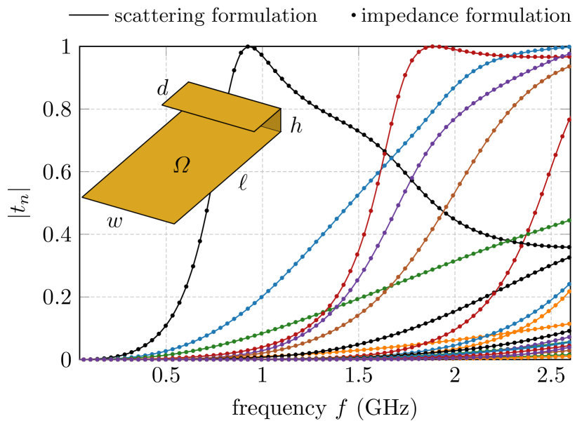
Figure 1: Modal significances $|t_{n}|$ computed for a PEC geometry adapted from [9]. The dimensions read $\ell=120\,\mathrm{mm}$, $w=60\,\mathrm{mm}$, $h=15\,\mathrm{mm}$, and $d=30\,\mathrm{mm}$. Impedance-based formulation [3] and scattering-based formulation (1) are employed with $\mathbf{S}_{\mathrm{b}}$ being the unit matrix.

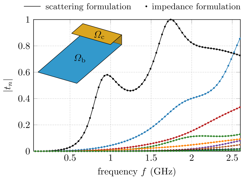
Figure 2: Modal significances $|t_{n}|$ computed for the substructure $\varOmega_{\mathrm{c}}$ in the presence of the background scatterer $\varOmega_{\mathrm{b}}$. Dimensions are identical to Fig. 1. The impedance-based method relies on formulation [9], while the scattering-based formulation relies on (1).

Previously, calculations like these were limited by their reliance on MoM [9, 23]. This paper demonstrates that substructure characteristic modes can be evaluated using the scattering matrix formalism, significantly expanding their scope and computational capabilities.

III Scattering Formulation of Substructure Characteristic Modes

Assume a controllable antenna region $\varOmega_{\mathrm{c}}$ and the surrounding (or background) region $\varOmega_{\mathrm{b}}$, as illustrated in Fig. 3. Let $\mathbf{S}_{\mathrm{b}}$ denote that scattering matrix [21, 20] for the background region $\varOmega_{\mathrm{b}}$, which connects incoming waves represented by coefficients collected in a vector $\mathbf{a}$ into outgoing waves represented by a vector $\mathbf{f}$. Similarly, let $\mathbf{S}$ denote the scattering matrix for the composite object $\varOmega_{\mathrm{c}}\bigcup\varOmega_{\mathrm{b}}$. The core hypothesis of this paper is that substructure characteristic modes are determined from the generalized eigenvalue problem

$$\mathbf{S}\mathbf{a}_{n}=s_{n}\mathbf{S}_{\mathrm{b}}\mathbf{a}_{n},$$ (1)

where $\mathbf{a}_{n}$ are characteristic excitations and $s_{n}$ characteristic scattering eigenvalues. Throughout the remainder of the paper, we refer to these quantities as characteristic modes due to their equivalence with the characteristic currents $\mathbf{I}_{n}$ typically used in impedance-based formulations [3, 5]. This formulation generalizes the one defined by [24] and developed in [5] for objects in free space, which implicitly considers the background scattering matrix $\mathbf{S}_{\mathrm{b}}$ to be an identity matrix. It also covers the special case studied for periodic structures in [25], where the background scattering matrix $\mathbf{S}_{\mathrm{b}}$ is related to an implicit connection between plane waves on either side of a scattering surface, analogous to the S-parameters of a transmission line network. The scattering eigenvalues $s_{n}$ are related to modal significance $|t_{n}|$ and characteristic eigenvalues $\lambda_{n}$ as [5]

$$t_{n}=\frac{s_{n}-1}{2}\quad\text{and }\lambda_{n}=-\operatorname{Im}\{t_{n}^{-1}\}=\mathrm{j}\frac{s_{n}+1}{s_{n}-1}.$$ (2)

Similarly to characteristic modes of isolated objects [5], for lossless objects, characteristic modes exhibit the following orthogonality relations

$$\mathbf{a}_{m}^{\mathrm{H}}\mathbf{a}_{n}=\delta_{mn},\quad\mathbf{f}_{m}^{\mathrm{H}}\mathbf{f}_{n}=\delta_{mn},$$ (3)

which, for example, translates to the orthogonality of characteristic far fields and where ^H denotes Hermitian transpose and $\delta_{mn}$ is the Kronecker delta. Equivalence between scattering and impedance formulations is supported by data shown in Figs. 1 and 2 comparing results from modal significances produced by (1) and an impedance-based formulation of substructure modes [9]. A mathematical derivation of this equivalence is outlined in Section IV and Appendix B.

Figure 3: Sketch of the physical interpretation of scattering matrices $\mathbf{S}_{\mathrm{b}}$ and $\mathbf{S}$.

III-A Variations

For lossless objects, the eigenvalue problem in (1) can be rearranged into several alternative forms. Scattering matrices are unitary for lossless objects [21], $\mathbf{S}^{\mathrm{H}}\mathbf{S}=\mathbf{1}$, leading to

$$\mathbf{S}_{\mathrm{b}}^{\mathrm{H}}\mathbf{S}\mathbf{a}_{n}=s_{n}\mathbf{a}_{n}\quad\text{and}\quad\mathbf{S}\mathbf{S}^{\mathrm{H}}_{\mathrm{b}}\mathbf{f}_{n}=s_{n}\mathbf{f}_{n},$$ (4)

where $\mathbf{f}_{n}=\mathbf{S}_{\mathrm{b}}\mathbf{a}_{n}=s_{n}^{\ast}\mathbf{S}\mathbf{a}_{n}$ represents the scattered field, $\mathbf{1}$ is the identity matrix, and ^∗ denotes complex conjugate. The two versions in (4) are equivalent and differ only in expressing the eigenvalue problem in incoming (excitation), $\mathbf{a}_{n}$, or outgoing (scattered or radiated), $\mathbf{f}_{n}$, waves. We note that the incident field $\mathbf{a}_{n}$ differ from the scattered field $\mathbf{f}_{n}$ except for the free-space case with $\mathbf{S}_{\mathrm{b}}=\mathbf{1}$ [5].

Formulation (4) can be implemented using transition matrices [20]

$$\mathbf{S}=2\mathbf{T}+\mathbf{1}\quad\text{and}\quad\mathbf{S}_{\mathrm{b}}=2\mathbf{T}_{\mathrm{b}}+\mathbf{1},$$ (5)

which allows for the analysis of substructure characteristic modes solely in terms of transition matrices and characteristic number $t_{n}$. These formulations read

$$(2\mathbf{T}_{\mathrm{b}}^{\mathrm{H}}\mathbf{T}+\mathbf{T}_{\mathrm{b}}^{\mathrm{H}}+\mathbf{T})\mathbf{a}_{n}=t_{n}\mathbf{a}_{n}$$ (6)

and

$$(2\mathbf{T}\mathbf{T}_{\mathrm{b}}^{\mathrm{H}}+\mathbf{T}_{\mathrm{b}}^{\mathrm{H}}+\mathbf{T})\mathbf{f}_{n}=t_{n}\mathbf{f}_{n}$$ (7)

and does not follow a scheme analogous to the characteristic modes of isolated objects [5]. In contrast to (1), relations (4), (6), and (7) enable iterative matrix-free evaluation [8], an important factor when employing generic electromagnetic solvers for evaluating substructure characteristic modes for large problems. Details of the iterative solution is found in Appendix A. Moreover, relation (6) allows for interpreting the substructure scattered power as a power of the difference between the scattered field of the composite object $\mathbf{T}\mathbf{a}_{n}$ and the scattered field of the background $\mathbf{T}_{\mathrm{b}}\mathbf{a}_{n}$, i.e.

$$\frac{1}{2}|(\mathbf{T}-\mathbf{T}_{\mathrm{b}})\mathbf{a}_{n}|^{2}=\frac{-\operatorname{Re}\{t_{n}\}}{2}|\mathbf{a}_{n}|^{2}=\frac{1}{2}|t_{n}|^{2}|\mathbf{a}_{n}|^{2}$$ (8)

with the interpretation of no substructure scattering for $t_{n}=0$ (or $s_{n}=1$) and maximum scattering for $t_{n}=s_{n}=-1$ similar to the free-space case [5]. Here, we have utilized the property [5] $\mathbf{T}^{\mathrm{H}}\mathbf{T}=-\mathrm{Re}\{\mathbf{T}\}$.

IV Equivalence Between MoM and Scattering-Based Substructure Characteristic modes

The proposed formula (1) is equivalent to the impedance-based substructure modes [9], wherein a structure is separated into two (possibly connected) regions $\varOmega_{\mathrm{b}}$ (“background”) and $\varOmega_{\mathrm{c}}$ (“controllable”) and excitation is restricted to only the controllable region $\varOmega_{\mathrm{c}}$. A general scattering problem in the standard notation for electric field integral equation (EFIE)-formulations [18] reads

$$\mathbf{V}=\mathbf{Z}\mathbf{I},$$ (9)

where $\mathbf{V}$ is an excitation vector, $\mathbf{Z}$ is the impedance matrix associated with the scatterer $\varOmega$, and $\mathbf{I}$ is an induced current density, all represented in a particular basis. Bifurcating the system into subsets of the basis functions associated with the two regions $\varOmega_{\mathrm{b}}$ and $\varOmega_{\mathrm{c}}$ and enforcing zero excitation on the background region leads to [14]

$$\mathbf{Z}\mathbf{I}=\begin{bmatrix}\mathbf{Z}_{\mathrm{b}\mathrm{b}}&\mathbf{Z}_{\mathrm{b}\mathrm{c}}\\ \mathbf{Z}_{\mathrm{c}\mathrm{b}}&\mathbf{Z}_{\mathrm{c}\mathrm{c}}\end{bmatrix}\begin{bmatrix}\mathbf{I}_{\mathrm{b}}\\ \mathbf{I}_{\mathrm{c}}\end{bmatrix}=\begin{bmatrix}\mathbf{0}\\ \mathbf{V}_{\mathrm{c}}\end{bmatrix}.$$ (10)

By reducing the MoM system $\mathbf{Z}=\mathbf{R}+\mathrm{j}\mathbf{X}$ to its Schur complement, the substructure characteristic modes are defined as [9]

$$\widetilde{\mathbf{X}}\mathbf{I}_{\mathrm{c}n}=\lambda_{n}\widetilde{\mathbf{R}}\mathbf{I}_{\mathrm{c}n}\quad\text{or}\quad\widetilde{\mathbf{Z}}\mathbf{I}_{\mathrm{c}n}=(1+\mathrm{j}\lambda_{n})\widetilde{\mathbf{R}}\mathbf{I}_{\mathrm{c}n},$$ (11)

where $\widetilde{\mathbf{Z}}=\widetilde{\mathbf{R}}+\mathrm{j}\widetilde{\mathbf{X}}=\mathbf{Z}_{\mathrm{c}\mathrm{c}}-\mathbf{Z}_{\mathrm{c}\mathrm{b}}\mathbf{Z}_{\mathrm{b}\mathrm{b}}^{-1}\mathbf{Z}_{\mathrm{b}\mathrm{c}}$ is an impedance matrix related to the problem-specific numerical Green’s function [14]. This numerical Green’s function captures the field-generating behavior of currents on the controllable region $\varOmega_{\mathrm{c}}$ in the presence of the “background” region $\varOmega_{\mathrm{b}}$.

The proof of equality of (11) and (1) starts with factorization of the radiation matrix [26] $\mathbf{R}=\mathbf{U}_{1}^{\mathrm{T}}\mathbf{U}_{1}$, where the matrix $\mathbf{U}_{1}$ projects MoM basis functions onto spherical waves. Next step is partitioning $\mathbf{U}_{1}=\begin{bmatrix}\mathbf{U}_{1\mathrm{b}}&\mathbf{U}_{1\mathrm{c}}\end{bmatrix}$ and factorization

$$\widetilde{\mathbf{R}}=\widetilde{\mathbf{U}}_{1}^{\mathrm{H}}\widetilde{\mathbf{U}}_{1}$$ (12)

for the substructure case, where $\widetilde{\mathbf{U}}_{1}=\mathbf{U}_{1\mathrm{c}}-\mathbf{U}_{1\mathrm{b}}\mathbf{Z}_{\mathrm{b}\mathrm{b}}^{-1}\mathbf{Z}_{\mathrm{b}\mathrm{c}}$. A substructure eigenvalue problem for T-matrix

$$\widetilde{\mathbf{T}}\mathbf{f}_{n}=t_{n}\mathbf{f}_{n}$$ (13)

with $t_{n}=\left(1+\mathrm{j}\lambda_{n}\right)^{-1}$ can be formulated by substituting (12) into (11), left multiplication with $\widetilde{\mathbf{U}}_{1}\widetilde{\mathbf{Z}}^{-1}$ and by identifying

$$\widetilde{\mathbf{T}}=-\widetilde{\mathbf{U}}_{1}\widetilde{\mathbf{Z}}^{-1}\widetilde{\mathbf{U}}_{1}^{\mathrm{H}}\quad\mathrm{and}\quad\mathbf{f}_{n}=-\widetilde{\mathbf{U}}_{1}\mathbf{I}_{\mathrm{c}n}.$$ (14)

Appendix B then shows that matrix $\widetilde{\mathbf{T}}$ equals to the matrix used in (7). Similarly to full characteristic modes, the characteristic substructure current can be evaluated as [5]

$$\mathbf{I}_{\mathrm{c}n}=t_{n}^{-1}\widetilde{\mathbf{Z}}^{-1}\widetilde{\mathbf{U}}_{1}^{\mathrm{H}}\mathbf{f}_{n}.$$ (15)

IV-A Example — Demonstrating equivalence

To demonstrate the numerical equivalence between the impedance and scattering formulations in (11) and (1), we employ a PEC structure reported in [9], which consists of a PIFA-like region connected to a finite ground plane, as depicted in the inset of Fig. 1. In Fig. 1, the characteristic modes of the full structure are computed without any separation into controllable and background regions, i.e., the entire region is controllable. Impedance and scattering operators are calculated using MoM, and the modal significances produced by the impedance and scattering formulations are numerically identical. Similarly, Fig. 2 displays modal significances when only part $\varOmega_{\mathrm{c}}$ of the structure is controllable (following [9]), and again the impedance (11) and scattering formulations (1) agree within numerical precision.

IV-B MoM & T-matrix hybrid

Hybridization of MoM and T-matrix techniques efficiently models complex inhomogeneous structures, so long as the regions described by each method can be separated by a plane [27]. Transition matrices can be computed for arbitrary background problems, but the computational acceleration over full MoM implementations is most pronounced when analytic forms of transition matrices can be employed, e.g., Mie series results for layered spherical structures or infinite ground planes. In this section, we discuss how this form of hybridization also allows for the efficient computation of substructure modes when part or all of the background region is represented by a transition matrix.

Consider a case from Fig. 2 to which a dielectric object is introduced as in Fig. 4. The scattering properties of a dielectric object can be efficiently described by matrix $\mathbf{T}_{\mathrm{\mathrm{b}1}}$, while the scattering properties of the metallic structure are described by the impedance matrix $\mathbf{Z}$ composed according to (10).

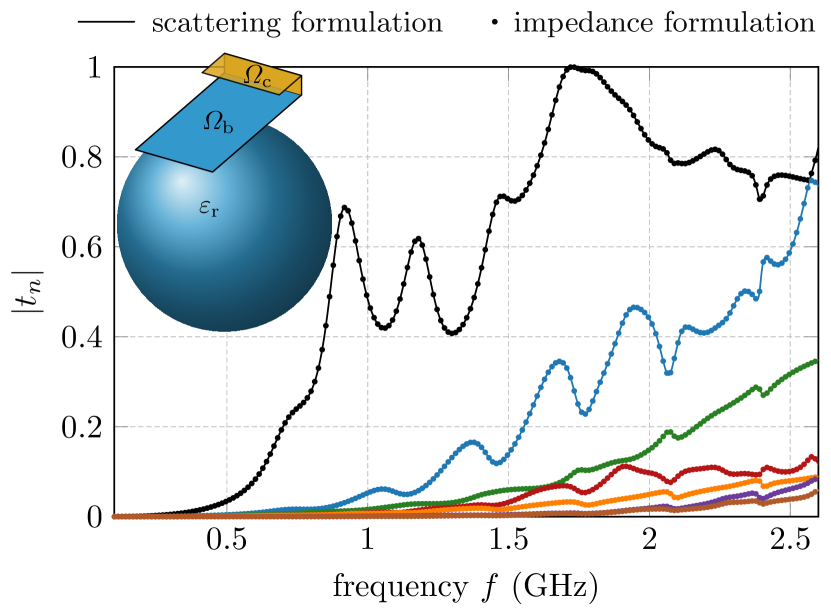
Figure 4: Modal significances $|t_{n}|$ computed for the substructure $\varOmega_{\mathrm{c}}$ in the presence of the background which contains scatterer $\varOmega_{\mathrm{b}}$ and a dielectric sphere filled with relative permittivity $\varepsilon_{\mathrm{r}}=4$. The diameter of the sphere equals 180 mm and the distance between the sphere and the metallic structure is 30 mm. Other dimensions are identical to Fig. 1. The impedance-based method relies on (11) and (16), while the scattering-based formulation relies on (1).

The reaction of the entire setup to an external excitation $\mathbf{a}^{\mathrm{i}}$ can be written as [27]

$$(\mathbf{Z}+\mathbf{U}^{\mathrm{T}}_{4}\mathbf{T}_{\mathrm{\mathrm{b}1}}\mathbf{U}_{4})\mathbf{I}=(\mathbf{U}_{1}^{\mathrm{T}}+\mathbf{U}_{4}^{\mathrm{T}}\mathbf{T}_{\mathrm{\mathrm{b}1}})\mathbf{a}^{\mathrm{i}}.$$ (16)

The matrix $\mathbf{Z}+\mathbf{U}^{\mathrm{T}}_{4}\mathbf{T}_{\mathrm{\mathrm{b}1}}\mathbf{U}_{4}$ is the impedance matrix of a metallic body in the presence of a dielectric object, with the second term being interpreted as a contribution of matrix $\mathbf{T}_{\mathrm{\mathrm{b}1}}$ to the background Green’s function [16]. Characteristic decomposition of this modified impedance matrix gives a spectrum similar to Fig. 1, with the entire conducting region in the presence of a dielectric sphere [28]. On the other hand, if substructure modes solely excitable from region $\varOmega_{\mathrm{c}}$ are desired, then this matrix is further modified and decomposed according to (11). The resulting spectrum of modal significances, where the entire region $\varOmega_{\mathrm{b}}$ is considered a background, is shown in Fig. 4. The equivalence of this formulation to (1) is demonstrated in the same figure.

IV-C Infinite ground plane

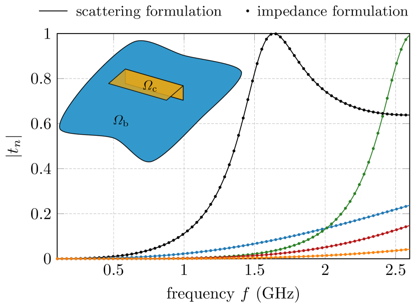
Figure 5: Modal significances $|t_{n}|$ computed for the substructure $\varOmega_{\mathrm{c}}$ in the presence of the background $\varOmega_{\mathrm{b}}$, which in this case is an infinite perfectly conducting ground plane. Dimensions are identical to Fig. 1.

An extreme version of the structure studied in Fig. 2 is a region $\varOmega_{\mathrm{c}}$ placed above an infinitely large perfectly conducting plane as depicted in Fig. 5. When substructure characteristic modes are evaluated in this scenario, a common practice is to construct and decompose the matrix $\widetilde{\mathbf{Z}}_{\mathrm{c}\mathrm{c}}$ for the region $\varOmega_{\mathrm{c}}$ using the Green’s function based on equivalent image currents [11]. Another possibility is to decompose the impedance matrix belonging to region $\varOmega_{\mathrm{c}}$ and its mirror image and then employ point symmetries [29] to filter out modes belonging to irreducible representation with even parity (those would belong to a perfectly magnetically conducting ground plane).

Within the scattering formulation (1), the problem is solved by adding an image of region $\varOmega_{\mathrm{c}}$ and an image of the incident field. This results in a total electric field with vanishing tangential components at the ground plane $\varOmega_{\mathrm{b}}$. The symmetry of the incident field eliminates half of the spherical waves. Specifically, only spherical waves exhibiting electric dipole moment normal to the ground plane and tangential magnetic dipole moment remain. For example, placing the ground plane $\varOmega_{\mathrm{b}}$ in the $xy$ plane and denoting $l,m$ the degree and azimuthal numbers, respectively, only TE spherical waves with even $l+m$ and TM spherical waves with odd $l+m$ remain. The equivalence of the impedance-based formulation and scattering formulation is presented in Fig. 5.

The practicality of using substructure characteristic modes is demonstrated by comparing spectra from Figs. 2, 4 and 5. In all cases, the black resonance peak appearing between $1.5\,\mathrm{GHz}$ and $2\,\mathrm{GHz}$ can be identified but would be lost if full characteristic decomposition was made, cf., Fig. 1. This resonance belongs to a mode responsible for the PIFA operation, and substructure decompositions show how it is affected by a particular background.

V Utilization of Arbitrary Full-Wave Solver

In case no in-house code is available to construct scattering matrices $\mathbf{S}$ and $\mathbf{S}_{\mathrm{b}}$, commercial simulators can be employed instead. This requires an interface between the simulator and a post-processor to assemble and decompose the scattering matrices.

To demonstrate the flexibility of scattering formulation (1), the scattering dyadic matrices [7] are employed in this section to evaluate sub-structure characteristic modes on several complex examples using a commercial solver as the core computational engine. To mitigate the computational burden stemming from the fact that the full-wave evaluation is repetitively performed for all columns of the scattering dyadic matrices, an iterative procedure [8] is employed and modified for the substructure case, see Appendix A. Codes for these examples implemented in MATLAB and Altair FEKO [30] are available at [31].

V-A Planar Inverted-F Antennas

A PIFA of the same dimensions as in Fig. 1 is studied once more, now with the addition of two example configurations of the dielectric substrate. Modal significance data for these examples, along with the previously studied PEC-only model, are shown in Fig. 6.

The reference case (PIFA #1) is made solely of PEC and represented by black traces. This case serves only as a verification of the scattering dyadic matrix procedure [7]. The resulting data are indistinguishable from the curves in Fig. 2. The two cases involving dielectrics are also shown in Fig. 6 and include two configurations of a lossless dielectric material with relative permittivity $\varepsilon_{\mathrm{r}}=2.33$. One case (PIFA #2) is built with two thin (1.575 mm) dielectric layers backing the parallel conductive layers in the PIFA system. The other case (PIFA #3) includes a dielectric block spanning the entire space between the ground plane and the upper motif.

It can be seen that the eigen-traces of PIFA #1 and PIFA #2 are comparable, which is given by the fact that thin substrate minimizes the effect of the dielectrics, i.e., the effective permittivity between the ground plane and the upper motif is close to unity, leading to only a slight downward shift in the resonant frequency of the dominant characteristic mode. This is not the case with PIFA #3, which behaves both qualitatively and quantitatively differently. The modal significance maxima are considerably shifted towards lower frequencies due to the reduced wavelength within the dielectric. The shape of the trace associated with the dominant mode is also visually quite different.

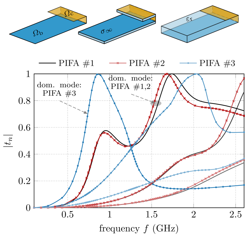
Figure 6: The first three substructure characteristic modes for different planar F antennas. The first model is taken from Fig. 2 and serves as a verification. The second model is built on a substrate with a thickness of 1.575 mm and relative permittivity $\varepsilon_{\mathrm{r}}=2.33$. The third model has a dielectric block of $\varepsilon_{\mathrm{r}}=2.33$ filling the space between the ground plane and the antenna. All models are lossless and treated with an iterative algorithm that employs surface equivalence method-of-moment from Altair FEKO [30]. The traces were adaptively refined to obtain smooth curves with relatively few samples.

V-B Simplified CubeSat Model

The previous example demonstrates the quantitative effect of dielectric substrates on modal characteristics of a PIFA, which can, to a certain extent, be anticipated from general rules of antenna design, i.e., shifting of resonances to lower frequencies through the use of dielectric loading. In this final example, however, we consider the modal characteristics of a complex system for which limited engineering intuition can be applied a priori.

The substructure characteristic modes of a simplified CubeSat model are evaluated in Fig. 7. The CubeSat frame of dimensions $10\times 10\times 15$ cm³ (approximately 1.5U format [32]) is formed by a PEC strip of width 1 cm. The frame is galvanically connected with the solid PEC top cover and left open on the underside. The interior is filled with a dielectric material with relative permittivity $\varepsilon_{\mathrm{r}}=3$. The PIFA of dimensions $w=5$ cm, $d=2.5\,$cm, and $h=1.25\,$cm is mounted on the top of the CubeSat and, similarly as in Fig. 2, only this antenna region is considered controllable for modal analysis, see the inset in Fig. 7. Notice the antenna size was reduced by 20% as compared to Fig. 2 to reflect the change of the ground plane size (from 120 cm to 100 cm) in this example, following dimensions of standard CubeSats. The model is lossless and treated with an iterative algorithm that employs surface equivalence method-of-moment from Altair FEKO [30]. The traces were adaptively refined to obtain smooth curves with relatively few samples.

The spectrum shown in Fig. 7 is dominated by only one mode, an observation agreeing well with the similar arrangement in Fig. 2. Considering the 20% relative size reduction of PIFA in Fig. 7 as compared with Fig. 2, the dominant mode resonates at comparable frequency. The background structure contains a large dielectric block with many internal resonances (approximately 80 cavity resonances between 0.1 GHz and 2.6 GHz). Nevertheless, all these resonances are filtered out by the substructure formulation (1). The only exception is the mode having an abrupt increase of modal significance around 1.6 GHz. This spike is still well-modeled by the iterative algorithm by finely sampling the frequency axis.

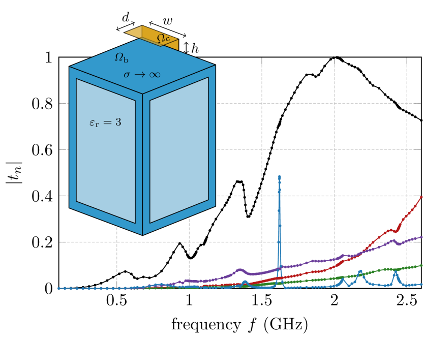
Figure 7: The first five substructure characteristic modes for a simplified model of a CubeSat. The CubeSat has dimensions $10\times 10\times 15$ cm³. The frame is made of PEC and has a width of 1 cm. The top cover is also made of PEC and forms a ground plane for a PIFA mounted on the CubeSat. The PIFA has dimensions of $w=5$ cm, $d=2.5$ cm, $h=1.25$ cm, and is the only controllable region in the model. The entire CubeSat is filled with dielectrics of relative permittivity $\varepsilon_{\mathrm{r}}=3$.

VI Discussion

The theoretical developments and set of examples provided in previous sections thoroughly demonstrate that the scattering formulation of substructure characteristic modes (1) is able to reproduce cases treated using classical formulation [9], while also allowing for the analysis of arbitrarily complex material distributions without modifying the evaluation procedure.

With the exception of the CubeSat example shown in Fig. 7, all examples are based on the same PIFA-like controllable region in the presence of varying backgrounds. Substantial differences between the resulting modal characteristics in each example clearly illuminate the high potential impact of background objects on modal performance. This is particularly noticeable in Fig. 6, where the inclusion of thin dielectric support layers leads to non-negligible changes in modal significance. If outputs from characteristic mode analyses are used in the design of antennas, it is therefore critical to fully model any background objects, including dielectrics, rather than using simplified background models and small perturbation approximations. The approach presented in this manuscript facilitates this rigorous analysis.

To further investigate the potential of the scattering formulation, it is worth considering the scenarios depicted in Fig. 8. All the cases treated in Sections II, IV and V solely dealt with panel (a), in which controllable and background regions might share a boundary but are otherwise disjoint.

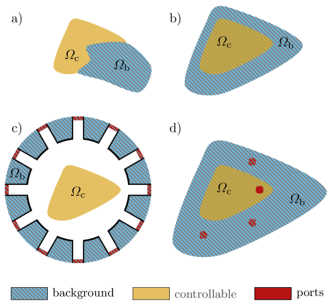
Figure 8: Illustrations of different setups to be considered for decomposition via substructure characteristic modes. (a) Classical arrangement with non-overlapping (possibly connected) regions. (b) Region $\varOmega_{\mathrm{c}}$ partly or fully overlapping with background region $\varOmega_{\mathrm{b}}$. (c) Region $\varOmega_{\mathrm{b}}$ in a cavity and $\varOmega_{\mathrm{c}}$ also contains waveguide ports. (d) Region $\varOmega_{\mathrm{c}}$ overlapping with background material in the presence of ports. Regions $\varOmega_{\mathrm{c}}$ and $\varOmega_{\mathrm{b}}$ are composed of arbitrary material distributions.

The first generalization is shown in panel (b), where controllable and background regions share the same volumes yet have different material properties. The meaning of such a situation can be understood from the volume equivalence principle. When building an equivalent description of a given scattering scenario, one can choose which part of polarization belongs to equivalent sources and which belongs to a background. In such a case, the controllable region is not a physical structure but a contrast between two material distributions. In principle, this scenario can be approached by classical treatment using a partial background Green’s function, however, the computation overhead will be considerable. On the other hand, within the scattering formulation, the problem from panel (b) is treated exactly like the problem from panel (a), i.e., by separately evaluating scattering from the entire system and the background.

The second generalization is the addition of ports, a situation depicted in panel (c). A possible scenario might be a substructure problem of Section II, where a port is added to controllable degrees of freedom. Although proposals exist for evaluating characteristic modes on antennas loaded by ports [33], we stress here that the ports present no qualitative change for the scattering formulation. Furthermore, the scattering formulation suggests that substructure characteristic modes can be evaluated even for circuits [21]. For example, the scattering matrices $\mathbf{S}_{\mathrm{b}}$ might represent a circuit without a particular region, which will be considered the controllable part.

Lastly, panel (d) of Fig. 8 combines all preceding scenarios. A possible application of this scenario is the analysis and optimization of minimum scattering antenna [34] by inspecting characteristic modes and their significance [35], or techniques involving generalized scattering matrix [36, 37]. In such a case, the substructure characteristic modes are not reachable via the Schur complement method [9], and their formulation will be challenging if background Green’s function is employed. Yet, the scattering formulation stays always the same, solely demanding to evaluate scattering matrices $\mathbf{S}$ and $\mathbf{S}_{\mathrm{b}}$ for a situation with and without the controllable part of the structure.

VII Conclusion

The method proposed in this paper extends the scattering-based formulation of characteristic modes to general substructure problems. Such problems were previously limited to cases where numerical or analytical problem-specific (non-free-space) Green’s functions are known, typically by way of Schur complement methods based on the method of moments. Using the proposed extension of scattering-based characteristic mode analysis, this requirement is lifted, and characteristic modes for all linear problems with arbitrary structure/substructure designations can be analyzed.

The examples throughout the paper demonstrate the flexibility of the method through its application to a family of problems based on a PIFA-like antenna above a finite ground plane. The resulting data demonstrate equivalence between the proposed method and impedance-based formulations, and highlight the generality of the approach to variations involving large dielectric background media, infinite ground planes, and finite dielectric regions. Further discussion regarding its application to problems involving wave ports and acceleration using iterative algorithms points to several areas for continued research, with the general direction aiming toward the fast and efficient characteristic mode analysis of antennas and scatterers in highly complex, arbitrary material environments.

Appendix A Matrix-Free Evaluation of Substructure Characteristic Modes

Characteristic modes can be evaluated efficiently using an iterative matrix-free algorithm [8]. Instead of having full, explicit knowledge of a matrix being decomposed, these algorithms rely on knowing the result of a matrix-vector multiplication of that matrix with an arbitrary vector. In the case of characteristic modes, the matrix itself is a scattering operator, while the matrix-vector multiplication represents the solution to a scattering problem for a particular excitation. Nevertheless, algorithms such as Arnoldi iteration used in [8] are not suitable for generalized eigenvalue problems, such as (1). Therefore, to evaluate substructure characteristic modes in a matrix-free fashion, the formulations (4), (6) and (7) are used. Furthermore, it is important to realize that only results of multiplications $\mathbf{T}\mathbf{x},\mathbf{T}_{\mathrm{b}}\mathbf{x},\mathbf{S}\mathbf{x},\mathbf{S}_{\mathrm{b}}\mathbf{x}$ are accessible via general purpose electromagnetic solvers. When adapting the algorithms described in [8], the following changes in the desired matrix-vector products are made

$$\mathbf{S}_{\mathrm{b}}^{\mathrm{H}}\mathbf{S}\mathbf{a}_{n} =\left(\mathbf{S}_{\mathrm{b}}\left(\mathbf{S}\mathbf{a}_{n}\right)^{*}\right)^{*}$$ (17)

$$(2\mathbf{T}_{\mathrm{b}}^{\mathrm{H}}\mathbf{T}+\mathbf{T}_{\mathrm{b}}^{\mathrm{H}}+\mathbf{T})\mathbf{a}_{n} =\left(\mathbf{T}_{\mathrm{b}}\left(\mathbf{a}_{n}+2\mathbf{T}\mathbf{a}_{n}\right)^{*}\right)^{*}+\mathbf{T}\mathbf{a}_{n}$$

where it was assumed that scattering, as well as transition matrices, are symmetric and where only formulations involving excitation vectors $\mathbf{a}_{n}$ are shown for brevity.

Algorithm 1 Matrix-free algorithm

1: $m=0$

2: $\mathbf{a}_{\mathrm{b}}\leftarrow\mathrm{rand}$

3:while stopping criteria are not met do

4:     $\mathbf{a}_{m}\leftarrow\mathbf{a}_{m}/|\mathbf{a}_{m}|$

5:      modified Gram-Schmidt procedure over $\{\mathbf{a}_{m}\}$

6:      $\mathbf{f}_{1m}\leftarrow\mathbf{M}\mathbf{a}_{m}$

7:      $\widehat{\mathbf{a}}\leftarrow\mathbf{P}\left(\mathbf{a}_{m}+2\mathbf{f}_{1m}\right)^{*}$

8:      $\widehat{\mathbf{f}}_{2m}\leftarrow\mathbf{M}_{\mathrm{b}}\widehat{\mathbf{a}}$

9:      $\mathbf{f}_{m}\leftarrow\mathbf{f}_{1m}+\mathbf{P}\widehat{\mathbf{f}}_{2m}^{\ast}$

10:      $\mathbf{A}_{m}\leftarrow\sum_{p\leq m}\mathbf{f}_{p}\mathbf{a}_{p}^{\mathrm{H}}$

11:      $\{t_{n}\}_{m}\leftarrow\mathrm{eig}(\mathbf{A}_{m})$

12:      $\mathbf{P}_{m}\leftarrow\sum_{p\leq m}\mathbf{a}_{p}\mathbf{a}_{p}^{\mathrm{H}}$

13:      $\mathbf{a}_{m+1}\leftarrow\mathbf{f}_{m}-\mathbf{P}_{m}\mathbf{f}_{m}$

14:     $m\leftarrow m+1$

15:end while

An example of the procedure used to estimate substructure characteristic modes using transition matrices in matrix-free manner is sketched in Algorithm 1, where $\mathbf{M}=\mathbf{T}$, $\mathbf{M}_{\mathrm{b}}=\mathbf{T}_{\mathrm{b}}$, $\mathbf{A}=2\mathbf{T}_{\mathrm{b}}^{\mathrm{H}}\mathbf{T}+\mathbf{T}_{\mathrm{b}}^{\mathrm{H}}+\mathbf{T}$ abbreviates the matrix to be decomposed, and $\mathbf{P}=\mathbf{I}$ is an identity matrix. The algorithm is stopped when magnitude $\left|\mathbf{a}_{m+1}\right|$ is sufficiently small or relative changes in estimated eigenvalues $t_{n}$ are sufficiently small. Steps no. 5 and 6 are the solutions to scattering problems involving full structure and background, respectively, and can be obtained from any full-wave electromagnetic solver. The modified Gram–Schmidt procedure is used in Algorithm 1 to assure its stability [38].

Another possibility to evaluate substructure characteristic modes is to employ scattering dyadic matrices, accessible with arbitrary electromagnetic solver [7]. In this case, the matrices $\tilde{\mathbf{S}}$ and $\tilde{\mathbf{S}}_{\mathrm{b}}$ are defined as in [7, eq. (21)] and denoted here as scattering and background scattering dyadic matrices, respectively. The matrices are not transposed symmetric [7, eq. (4)], so the Algorithm 1 must be modified by settings $\mathbf{M}=\tilde{\mathbf{S}}$, $\mathbf{M}_{\mathrm{b}}=\tilde{\mathbf{S}}_{\mathrm{b}}$, and with matrix $\mathbf{P}$ being indexing matrix containing zeros except positions $P_{pq}$ and $P_{pq}$ where pairs of the quadrature points are mapped as

$$P_{pq}=P_{pq}=1\Longleftrightarrow\hat{\boldsymbol{r}}_{p}=-\hat{\boldsymbol{r}}_{q}.$$ (18)

In addition, matrix $\mathbf{P}$ is further modified by flipping the $\pm$ sign for respective positions where the quadrature points in $\vartheta$-polarization block of the dyadic lie on $\pm z$ axis, and for all entries corresponding to $\varphi$-polarization block except of points lying on $\pm z$ axis.

Appendix B Equivalence Between MoM-based and Scattering-Based Substructure Characteristic Modes

The modified transition matrix (14) resembles the transition matrix-based expression in [5] with the difference that the spherical wave matrix $\widetilde{\mathbf{U}}$ is complex-valued. Rewriting (14) using block matrices (10) produces

$$\widetilde{\mathbf{T}}=\mathbf{U}_{1}\begin{bmatrix}-\mathbf{Z}_{\mathrm{b}\mathrm{b}}^{-1}\mathbf{Z}_{\mathrm{b}\mathrm{c}}\widetilde{\mathbf{Z}}^{-1}\mathbf{Z}_{\mathrm{b}\mathrm{c}}^{\mathrm{H}}\mathbf{Z}_{\mathrm{b}\mathrm{b}}^{-\mathrm{H}}&\mathbf{Z}_{\mathrm{b}\mathrm{b}}^{-1}\mathbf{Z}_{\mathrm{b}\mathrm{c}}\widetilde{\mathbf{Z}}^{-1}\\[5.0pt] \widetilde{\mathbf{Z}}^{-1}\mathbf{Z}_{\mathrm{b}\mathrm{c}}^{\mathrm{H}}\mathbf{Z}_{\mathrm{b}\mathrm{b}}^{-\mathrm{H}}&-\widetilde{\mathbf{Z}}^{-1}\end{bmatrix}\mathbf{U}_{1}^{\mathrm{T}}$$ (19)

which partly resembles a block inversion of the MoM matrix (10) except for some Hermitian transposes.

To express the transition matrices of the composite object $\varOmega$ and background object $\varOmega_{\mathrm{b}}$ in MoM system matrices, we use [5]

$$\mathbf{T}=-\mathbf{U}_{1}\mathbf{Z}^{-1}\mathbf{U}_{1}^{\mathrm{T}}\quad\text{and }\mathbf{T}_{\mathrm{b}}=-\mathbf{U}_{1}\begin{bmatrix}\mathbf{Z}_{\mathrm{b}\mathrm{b}}^{-1}&\mathbf{0}\\ \mathbf{0}&\mathbf{0}\end{bmatrix}\mathbf{U}_{1}^{\mathrm{T}}.$$ (20)

Substituting these T-matrices into (7) and using block matrix inversion together with algebraic manipulations outlined below we realize that (11), (13), (7) are all identical.

The derivation starts with reformulation of (7) in MoM matrices

$$2\mathbf{T}\mathbf{T}^{\mathrm{H}}_{\mathrm{b}}+\mathbf{T}_{\mathrm{b}}^{\mathrm{H}}+\mathbf{T}\\ =\mathbf{U}_{1}\mathbf{Z}^{-1}\left(2\mathbf{R}\begin{bmatrix}\mathbf{Z}_{\mathrm{b}\mathrm{b}}^{-\mathrm{H}}&\mathbf{0}\\ \mathbf{0}&\mathbf{0}\end{bmatrix}-\mathbf{Z}\begin{bmatrix}\mathbf{Z}_{\mathrm{b}\mathrm{b}}^{-\mathrm{H}}&\mathbf{0}\\ \mathbf{0}&\mathbf{0}\end{bmatrix}-\mathbf{1}\right)\mathbf{U}_{1}^{\mathrm{T}},$$ (21)

where $\mathbf{R}=\mathbf{U}_{1}^{\mathrm{T}}\mathbf{U}_{1}$ has been used [26]. Realizing further that $2\mathbf{R}=\mathbf{Z}+\mathbf{Z}^{\mathrm{H}}$ for lossless scatterers, the relation simplifies to

$$2\mathbf{T}\mathbf{T}^{\mathrm{H}}_{\mathrm{b}}+\mathbf{T}_{\mathrm{b}}^{\mathrm{H}}+\mathbf{T}=\mathbf{U}_{1}\mathbf{Z}^{-1}\left(\mathbf{Z}^{\mathrm{H}}\begin{bmatrix}\mathbf{Z}_{\mathrm{b}\mathrm{b}}^{-\mathrm{H}}&\mathbf{0}\\ \mathbf{0}&\mathbf{0}\end{bmatrix}-\mathbf{1}\right)\mathbf{U}_{1}^{\mathrm{T}}\\ =\mathbf{U}_{1}\mathbf{Z}^{-1}\begin{bmatrix}\mathbf{0}&\mathbf{0}\\ \mathbf{Z}_{\mathrm{b}\mathrm{c}}^{\mathrm{H}}\mathbf{Z}_{\mathrm{b}\mathrm{b}}^{-\mathrm{H}}&-\mathbf{1}\end{bmatrix}\mathbf{U}_{1}^{\mathrm{T}}.$$ (22)

The final step is the use of block matrix inversion

$$\mathbf{Z}^{-1}=\begin{bmatrix}\mathbf{Z}_{\mathrm{b}\mathrm{b}}^{-1}+\mathbf{Z}_{\mathrm{b}\mathrm{b}}^{-1}\mathbf{Z}_{\mathrm{b}\mathrm{c}}\widetilde{\mathbf{Z}}^{-1}\mathbf{Z}_{\mathrm{c}\mathrm{b}}\mathbf{Z}_{\mathrm{b}\mathrm{b}}^{-1}&-\mathbf{Z}_{\mathrm{b}\mathrm{b}}^{-1}\mathbf{Z}_{\mathrm{b}\mathrm{c}}\widetilde{\mathbf{Z}}^{-1}\\[5.0pt] -\widetilde{\mathbf{Z}}^{-1}\mathbf{Z}_{\mathrm{c}\mathrm{b}}\mathbf{Z}_{\mathrm{b}\mathrm{b}}^{-1}&\widetilde{\mathbf{Z}}^{-1}\end{bmatrix}$$ (23)

which is identical to $\widetilde{\mathbf{T}}$ in (19)

$$2\mathbf{T}\mathbf{T}^{\mathrm{H}}_{\mathrm{b}}+\mathbf{T}_{\mathrm{b}}^{\mathrm{H}}+\mathbf{T}=\widetilde{\mathbf{T}}$$ (24)

proving that (11), (13), (7) are the same.

Notice that the above derivation demanded lossless scatterer. For lossy cases, matrix $\widetilde{\mathbf{R}}$ differs from the radiation operator $\widetilde{\mathbf{U}}_{1}^{\mathrm{H}}\widetilde{\mathbf{U}}_{1}$. For the special case with lossless background, the scattering-based formulation of characteristic modes is identical to the $\widetilde{\mathbf{Z}}$-formulation on the right in (11).

Mats Gustafsson received the M.Sc. degree in Engineering Physics 1994, the Ph.D. degree in Electromagnetic Theory 2000, was appointed Docent 2005, and Professor of Electromagnetic Theory 2011, all from Lund University, Sweden. He co-founded the company Phase holographic imaging AB in 2004. His research interests are in scattering and antenna theory and inverse scattering and imaging. He has written over 100 peer reviewed journal papers and over 100 conference papers. Prof. Gustafsson received the IEEE Schelkunoff Transactions Prize Paper Award 2010, the IEEE Uslenghi Letters Prize Paper Award 2019, and best paper awards at EuCAP 2007 and 2013. He served as an IEEE AP-S Distinguished Lecturer for 2013-15.

Lukas Jelinek was born in Czech Republic in 1980. He received his Ph.D. degree from the Czech Technical University in Prague, Czech Republic, in 2006. In 2015 he was appointed Associate Professor at the Department of Electromagnetic Field at the same university. His research interests include wave propagation in complex media, electromagnetic field theory, metamaterials, numerical techniques, and optimization.

Miloslav Capek (M’14, SM’17) received the M.Sc. degree in Electrical Engineering 2009, the Ph.D. degree in 2014, and was appointed a Full Professor in 2023, all from the Czech Technical University in Prague, Czech Republic. He leads the development of the AToM (Antenna Toolbox for Matlab) package. His research interests include electromagnetic theory, electrically small antennas, antenna design, numerical techniques, and optimization. He authored or co-authored over 160 journal and conference papers. Dr. Capek is the Associate Editor of IET Microwaves, Antennas & Propagation. He was a regional delegate of EurAAP between 2015 and 2020. He received the IEEE Antennas and Propagation Edward E. Altshuler Prize Paper Award 2023.

Johan Lundgren (M’22) is a postdoctoral researcher at Lund University. he received his M.Sc degree in engineering physics 2016 and Ph.D. degree in Electromagnetic Theory in 2021 all from Lund University, Sweden. His research interests are in electromagnetic scattering, wave propagation, computational electromagnetics, functional structures, meta-materials, inverse scattering problems, imaging, and measurement techniques.

Kurt Schab (S’09, M’16) is an Assistant Professor of Electrical Engineering at Santa Clara University, Santa Clara, CA USA. He received the B.S. degree in electrical engineering and physics from Portland State University in 2011 and the M.S. and Ph.D. degrees in electrical engineering from the University of Illinois at Urbana-Champaign in 2013 and 2016, respectively. From 2016 to 2018 he was a Postdoctoral Research Scholar at North Carolina State University in Raleigh, North Carolina. His research focuses on the intersection of numerical methods, electromagnetic theory, and antenna design.

References

- [1] C. G. Montgomery, R. H. Dicke, and E. M. Purcell, Principles of Microwave Circuits. New York, NY: McGraw-Hill, 1948.
- [2] R. Garbacz, “Modal expansions for resonance scattering phenomena,” Proc. IEEE, vol. 53, no. 8, pp. 856–864, Aug. 1965.
- [3] R. F. Harrington and J. R. Mautz, “Theory of characteristic modes for conducting bodies,” IEEE Trans. Antennas Propag., vol. 19, no. 5, pp. 622–628, 1971.
- [4] B. K. Lau, M. Capek, and A. M. Hassan, “Characteristic modes: Progress, overview, and emerging topics,” IEEE Antennas and Propagation Magazine, vol. 64, no. 2, pp. 14–22, 2022.
- [5] M. Gustafsson, L. Jelinek, K. Schab, and M. Capek, “Unified theory of characteristic modes: Part I–Fundamentals,” IEEE Trans. Antennas Propag., vol. 70, no. 12, pp. 11 801–11 813, 2022.
- [6] ——, “Unified theory of characteristic modes: Part II–Tracking, losses, and FEM evaluation,” IEEE Trans. Antennas Propag., vol. 70, no. 12, pp. 11 814–11 824, 2022.
- [7] M. Capek, J. Lundgren, M. Gustafsson, K. Schab, and L. Jelinek, “Characteristic mode decomposition using the scattering dyadic in arbitrary full-wave solvers,” IEEE Trans. Antennas Propag., vol. 71, no. 1, pp. 830–839, 2023.
- [8] J. Lundgren, K. Schab, M. Capek, M. Gustafsson, and L. Jelinek, “Iterative calculation of characteristic modes using arbitrary full-wave solvers,” IEEE Antennas Wireless Propag. Lett., vol. 22, no. 4, pp. 799–803, 2023.
- [9] J. Ethier and D. McNamara, “Sub-structure characteristic mode concept for antenna shape synthesis,” Electronics letters, vol. 48, no. 9, p. 1, 2012.
- [10] H. Alroughani, “An appraisal of the characteristic modes of composite objects,” Ph.D. dissertation, University of Ottawa (Canada), 2013.
- [11] G. Angiulli and G. Di Massa, “Scattering from arbitrarily shaped microstrip patch antennas using the theory of characteristic modes,” in IEEE Antennas and Propagation Society International Symposium and USNC/URSI National Radio Science Meeting, ser. APS-98. IEEE.
- [12] R. Zhao, Y. Lu, G. S. Cheng, W. Zhu, J. Hu, and H. Bagci, “Sub-structure characteristic mode analysis of microstrip antennas using a global multitrace formulation,” IEEE Trans. Antennas Propag., vol. 71, no. 12, pp. 10 026–10 031, 2023.
- [13] R. Luomaniemi, P. Ylä-Oijala, A. Lehtovuori, and V. Viikari, “Designing hand-immune handset antennas with adaptive excitation and characteristic modes,” IEEE Trans. Antennas Propag., vol. 69, no. 7, pp. 3829–3839, 2021.
- [14] P. Parhami, Y. Rahmat-Samii, and R. Mittra, “Technique for calculating the radiation and scattering characteristics of antennas mounted on a finite ground plane,” in Proceedings of the Institution of Electrical Engineers, vol. 124, no. 11. IET, 1977, pp. 1009–1016.
- [15] T. Cwik, J. Patterson, and T. Lockhart, “Constructing matrix Green’s functions for radiation and scattering problems,” in Digest on Antennas and Propagation Society International Symposium, 1989, pp. 586–589 vol.2.
- [16] Q. I. Dai, H. Gan, C. C. Weng, and C.-F. Wang, “Characteristic mode analysis using Green’s function of arbitrary background,” in 2016 IEEE International Symposium on Antennas and Propagation (APSURSI). IEEE, 2016, pp. 423–424.
- [17] A. Alakhras and D. McNamara, “Sub-structure characteristic mode computation utilising field-based MM/GTD hybrid methods,” Journal of Electromagnetic Waves and Applications, vol. 34, no. 13, pp. 1812–1821, 2020.
- [18] R. F. Harrington, Field Computation by Moment Methods. New York, NY: Macmillan, 1968.
- [19] H. Alroughani, J. L. T. Ethier, and D. A. McNamara, “On the classification of characteristic modes, and the extension of sub-structure modes to include penetrable material,” in 2014 International Conference on Electromagnetics in Advanced Applications (ICEAA). IEEE, 2014.
- [20] G. Kristensson, Scattering of Electromagnetic Waves by Obstacles. Edison, NJ: SciTech Publishing, an imprint of the IET, 2016.
- [21] D. M. Pozar, Microwave Engineering, 3rd ed. New York, NY: John Wiley & Sons, 2005.
- [22] M. I. Mishchenko, L. D. Travis, and D. W. Mackowski, “T-matrix computations of light scattering by nonspherical particles: A review,” J. Quant. Spectrosc. Radiat. Transfer, vol. 55, no. 5, pp. 535–575, 1996.
- [23] M. Capek and K. Schab, “Computational aspects of characteristic mode decomposition: An overview,” IEEE Antennas and Propagation Magazine, vol. 64, no. 2, pp. 23–31, 2022.
- [24] R. J. Garbacz and R. H. Turpin, “A generalized expansion for radiated and scattered fields,” IEEE Trans. Antennas Propag., vol. 19, no. 3, pp. 348–358, 1971.
- [25] K. Schab, F. W. Chen, L. Jelinek, M. Capek, J. Lundgren, and M. Gustafsson, “Characteristic modes of frequency-selective surfaces and metasurfaces from S-parameter data,” IEEE Trans. Antennas Propag., vol. 71, no. 12, pp. 9696–9706, 2023.
- [26] D. Tayli, M. Capek, L. Akrou, V. Losenicky, L. Jelinek, and M. Gustafsson, “Accurate and efficient evaluation of characteristic modes,” IEEE Trans. Antennas Propag., vol. 66, no. 12, pp. 7066–7075, 2018.
- [27] V. Losenicky, L. Jelinek, M. Capek, and M. Gustafsson, “Method of moments and T-matrix hybrid,” IEEE Trans. Antennas Propag., vol. 70, no. 5, pp. 3560–3574, 2022.
- [28] L. Jelinek, M. Gustafsson, K. Schab, M. Capek, and E. Moreno, “Transition matrix in characteristic modes theory,” in 2022 IEEE International Symposium on Antennas and Propagation and USNC-URSI Radio Science Meeting (AP-S/URSI). IEEE, jul 2022.
- [29] M. Masek, M. Capek, L. Jelinek, and K. Schab, “Modal tracking based on group theory,” IEEE Trans. Antennas Propag., vol. 68, no. 2, pp. 927–937, Feb. 2020.
- [30] (2022) Altair FEKO. Altair. [Online]. Available: https://www.altair.com/feko
- [31] M. Capek. (2024) Scattering dyadic characteristic modes (with Altair FEKO). [Online]. Available: https://github.com/kschab/scattering-dyadic-characteristic-modes/tree/main/FEM_MoM-FEKO
- [32] (2017) Cubesat 101 basic concepts and processes for first-time cubesat developers. National Aeronautics and Space Administration (NASA). [Online]. Available: https://www.nasa.gov/wp-content/uploads/2017/03/nasa_csli_cubesat_101_508.pdf
- [33] X. Deng, Y. Chen, and S. Yang, “Characteristic mode formulation for antennas with waveguide port feeding structures,” IEEE Antennas and Wireless Propagation Letters, vol. 20, no. 10, pp. 2063–2067, 2021.
- [34] W. Kahn and H. Kurss, “Minimum-scattering antennas,” IEEE Trans. Antennas Propag., vol. 13, no. 5, pp. 671–675, 1965.
- [35] P. Rogers, “Application of the minimum scattering antenna theory to mismatched antennas,” IEEE Trans. Antennas Propag., vol. 34, no. 10, pp. 1223–1228, 1986.
- [36] Y. G. Kim and S. Nam, “Determination of the generalized scattering matrix of an antenna from characteristic modes,” IEEE Trans. Antennas Propag., vol. 61, no. 9, pp. 4848–4852, 2013.
- [37] M. Alian and N. Noori, “A domain decomposition method for the analysis of mutual interactions between antenna and arbitrary scatterer using generalized scattering matrix and translation addition theorem of SWFs,” IEEE Trans. Antennas Propag., vol. 71, no. 10, p. 8088–8096, Oct. 2023.
- [38] G. H. Golub and C. F. van Loan, Matrix Computations, 4th ed. Baltimore, MD: The Johns Hopkins University Press, 2013.