Otto cycles with a quantum planar rotor

Abstract

We present two realizations of an Otto cycle with a quantum planar rotor as the working medium controlled by means of external fields. By comparing the quantum and the classical description of the working medium, we single out genuine quantum effects with regards to the performance and the engine and refrigerator modes of the Otto cycle. The first example is a rotating electric dipole subjected to a controlled electric field, equivalent to a quantum pendulum. Here we find a systematic disadvantage of the quantum rotor compared to its classical counterpart. In contrast, a genuine quantum advantage can be observed with a charged rotor generating a magnetic moment that is subjected to a controlled magnetic field. Here, we prove that the classical rotor is inoperable as a working medium for any choice of parameters, whereas the quantum rotor supports an engine and a refrigerator mode, exploiting the quantum statistics during the cold strokes of the cycle.

I Introduction

With the thermodynamic interpretation of the three level maser in 1959 [1], the field of quantum thermodynamics was born. Since then, quantum analogues of classical thermal machine models such as the Carnot cycle [2, 3, 4, 5, 6] and the Otto cycle [7, 8, 9, 10, 11, 12, 13] have been studied exhaustively. In these machines, the classical macroscopic working medium, usually a gas, is replaced by quantum systems of varying complexity that undergo a controlled cycle of strokes, which alternate between the thermal coupling with a hot and a cold reservoir and the modulation of the system Hamiltonian over time, mimicking the (model-extrinsic) motion of a “piston”. In this work, we focus on the Otto cycle, which can be operated both as an engine that outputs work at the expense of heat from the hot reservoir and as a refrigerator that extracts heat from the cold reservoir at the expense of work.

Studied quantum working media range from small finite-dimensional systems [14, 15, 16] to many-body systems [17, 18, 19] and infinite-dimensional continuous-variable systems [11, 20, 21]. Experimental proof-of-principle realizations of the Otto cycle were performed with trapped ions [22, 23], nano beams [24], nitrogen vacancy centers [25], spins with nuclear magnetic resonance techniques [26], optomechanical systems [27], quantum gases [28] and proposed for nanomechanical resonators[29], circuit QED [30], and quantum dots [31].

Continuous-variable working media naturally lend themselves to the study of quantum effects on the machine performance. They can represent motional degrees of freedom with a classical analogue, e.g. the position and momentum of a particle, admitting a direct comparison between the classical and the quantum version of the studied machine. Note however that the quantum-classical comparison is often understood as a comparison of machine models with and without coherence on a given quantum system [32, 33], provided that the periodic piston modulation affects the energy basis of the working medium. While the advantages of quantum machines are often highlighted in specific cases [34, 35, 36, 37], the performance of a machine model can in general both improve and deteriorate due to quantization of the working medium.

One predominantly studied working medium is the harmonic oscillator, due to its mathematically well-understood behaviour. Unfortunately, it was shown that the harmonic oscillator does not have the capacity for genuine quantum effects on the performance of a standard Otto cycle: a homogeneous scaling of the energy levels with respect to the work parameter $\lambda$ representing the periodic piston modulation of the harmonic frequency, $E_{n}(\lambda)=\lambda\hbar\omega(n+1/2)$ implies classical behavior [38]. Moreover, the same applies to any Otto cycle in which the cyclic modulation of the Hamiltonian implies a simple proportionality of the energy spectrum, $E_{n}(\lambda)\propto\lambda^{k}$.

Here we will consider the quantum planar rotor as a continuous-variable working medium for the quantum Otto cycle. This is in contrast to and a complement of previous theoretical works employing the rotor as an autonomous piston degree of freedom for engines [39, 40, 41, 42, 43]. Angular momentum quantization can lead to genuinely non-classical phenomena in the free evolution of a single planar rotor [44] as well as in the dynamics of coherently interlocked rotors [45]. Experimental demonstrations of rotor-based machines could be based on molecular rotors, the quantum dynamics of which is nowadays routinely observed and controlled with help of tailored laser pulses [46, 47] . Another platform to realize planar rotor analogues and rotor engines is circuit QED [48] , where the Josephson phase plays the role of the rotor angle. Finally, state-of-the-art experiments in levitated optomechanics with rigid nanorotors are steadily approaching the quantum regime [49, 50, 51, 52, 53].

We will formulate the theoretical model of a planar rotor subjected to an externally modulated potential in the four strokes of the paradigmatic Otto cycle (Section II) and investigate the classical and quantum predictions for two physically motivated examples, sketched in Fig. 1: The first one is a rotating electric dipole in the presence of an electric field of alternating strength in the plane of rotation (Section III). We show that the so defined Otto cycle, assuming ideal quenches of the electric field and full thermalization in between, always performs worse in the quantum case. Both the operation regimes as an engine or refrigerator and the energy output decrease in comparison to the classical case. The second example is a dipole in a magnetic field of alternating strength perpendicular to the rotation plane (Section IV). Here we show that the classical rotor operates neither as an Otto engine nor as a refrigerator, whereas the quantum rotor does, when the cold stroke of the Otto cycle is operated in the low-excitation regime. This constitutes a genuine advantage enabled by angular momentum quantization. We briefly conclude our study in Section V.

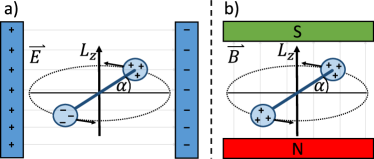
Figure 1: Two physical settings in which a planar rotor acts as the working medium of an Otto cycle: (a) Rotating electric dipole subject to an externally controlled, homogeneous electric field parallel to the rotation plane; (b) Charged rotor generating a magnetic dipole moment subject to a controlled magnetic field perpendicular to the rotation plane.

II Theoretical model

A planar rotor is a dynamical degree of freedom described by a single angular coordinate $\alpha\in[0,2\pi)$ and its conjugate angular momentum $L_{z}$. It represents the phase space of, for instance, a particle on a ring in the $xy$-plane, the phase variable in a superconducting Josephson loop, and the orientation of a rigid rotor on a fixed plane of rotation. We will first introduce the notation and theoretical description of a classical and quantum planar rotor, before briefly reviewing the ideal four-stroke Otto cycle.

II.1 Classical and quantum planar rotor

Classically, the canonical variables $(\alpha,L_{z})$ of the planar rotor can be treated in the same manner as the position and momentum of linear motion in one dimension. Physical states are described by phase-space probability densities $P(\alpha,L_{z})$ and valid (time-independent) Hamiltonians by $H(\alpha,L_{z})$, with the additional requirement of strict $2\pi$-periodicity in $\alpha$. We will consider Hamiltonians of the form

$$H=H(\alpha,L_{z})=\frac{(L_{z}-I\omega)^{2}}{2I}+V(\alpha),$$ (1)

with a given moment of inertia $I$, a periodic potential, $V(\alpha)=V(\alpha+2\pi)$, and an angular momentum displacement by $I\omega$. The latter can be viewed as a boost with respect to a rotating frame at angular frequency $\omega$.

The Gibbs state of such a classical planar rotor in thermal equilibrium at temperature $T$ is given by

$$P(\alpha,L_{z})=\frac{1}{Z}\mathrm{e}^{-H(\alpha,L_{z})/k_{\mathrm{B}}T},$$ (2)

with the partition function

$$Z = \int_{0}^{2\pi}\!\!\mathrm{d}\alpha\int_{-\infty}^{\infty}\!\!\mathrm{d}L_{z}\,\mathrm{e}^{-H(\alpha,L_{z})/k_{\mathrm{B}}T}$$ (3)

$$= \sqrt{2\pi Ik_{\mathrm{B}}T}\int_{0}^{2\pi}\!\!\mathrm{d}\alpha\,\mathrm{e}^{-V(\alpha)/k_{\mathrm{B}}T}.$$

In the quantum case, the differences between linear and rotational motion are more fundamental. The orientation state of the quantum planar rotor is described by $2\pi$-periodic wave functions $\psi(\alpha)=\langle\alpha|\psi\rangle$, and the periodicity implies that the angular momentum be quantized in integer multiples of $\hbar$. We can thus express the angular momentum operator as $\hat{L}_{z}=\sum_{m\in\mathbb{Z}}\hbar m\ket{m}\bra{m}$, defining the orthonormal basis of discrete angular momentum eigenstates, $\langle\alpha|m\rangle=\mathrm{e}^{im\alpha}/\sqrt{2\pi}$. The expansion coefficients of the wave function in this basis are obtained from its Fourier decomposition.

The conjugate angle operator $\hat{\alpha}$ can be defined through the unitary momentum displacement operators $\exp(ik\hat{\alpha})$, which for $k\in\mathbb{Z}$ adhere to the strict periodicity of the system and act like $\exp\left(ik\hat{\alpha}\right)\ket{m}=\ket{m+k}$. Consistently, the basis of angle states $|\alpha\rangle$ is obtained as

$$|\alpha\rangle=\sum_{m\in\mathbb{Z}}\frac{\mathrm{e}^{-im\alpha}}{\sqrt{2\pi}}|m\rangle.$$ (4)

They form a continuous orthonormal basis, $\langle\alpha_{1}|\alpha_{2}\rangle=\delta(\alpha_{1}-\alpha_{2}\mod 2\pi)$, and they are eigenstates of the displacement operators and thus of any periodic function of $\hat{\alpha}$ by virtue of the Fourier expansion; e.g., $V(\hat{\alpha})|\alpha\rangle=V(\alpha)|\alpha\rangle$. The canonical commutation relation between $\hat{L}_{z}$ and $\alpha$ can be expressed in terms of periodic functions as

$$\left[f(\hat{\alpha}),\hat{L}_{z}\right]=i\hbar f^{\prime}(\hat{\alpha}),\quad\forall\,\,2\pi\text{-periodic}\ f(\alpha).$$ (5)

The quantum version $\hat{H}$ of the generic Hamiltonian (1) will have a discrete spectrum of energy eigenvalues $E_{n}$. The corresponding Gibbs state is given by the density matrix $\hat{\gamma}=\exp(-\hat{H}/k_{\mathrm{B}}T)/Z$ with the quantum partition function $Z=\operatorname{tr}\{\exp(-\hat{H}/k_{\mathrm{B}}T)\}$.

For our following case studies and numerical computations, we conveniently introduce the rotational energy quantum as a natural energy scale,

$$E=\frac{\hbar^{2}}{I},$$ (6)

and express all relevant energies in units of this scale. When comparing the quantum and the classical rotor as a working medium, we expect notable differences only for thermal energies that do not exceed this scale by far.

II.2 Otto cycle

The Otto cycle is the most widely studied and instructive thermal machine model [11, 54], which can be generically formulated in a classical or quantum setting. We start with the quantum version and introduce the classical counterpart later. The basic setting comprises one hot and one cold thermal reservoir with respective temperatures $T_{h}>T_{c}$, and a quantum system acting as the working medium, whose Hamiltonian $\hat{H}(\lambda)$ depends on a control parameter $\lambda$. This parameter can be varied between two extreme values $\lambda_{h}$ and $\lambda_{c}$, which abstracts the cyclic motion of a piston. The temperature $T$ and the control parameter $\lambda$ are the two relevant independent state variables of the working medium.

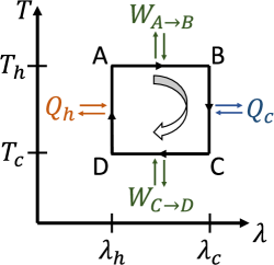
Figure 2: Phase diagram of the four-stroke Otto cycle with a generic working medium in terms of the temperature $T$ and the control parameter $\lambda$. The two horizontal lines represent the isentropic strokes in which the control parameter changes between $\lambda_{h}$ and $\lambda_{c}$ under work exchange. The two vertical lines represent “isochoric” thermalization of the working medium through heat exchange with a hot reservoir at temperature $T_{h}$ (left) and a cold reservoir at $T_{c}$ (right).

In its ideal implementation, the Otto cycle consists of four discrete strokes, as sketched in the phase diagram spanned by $\lambda$ and $T$ in Fig. 2: Two thermalization strokes ($B\to C$ and $D\to A$) in which the system is coupled to either reservoir of temperature $T_{h}$ or $T_{c}$ at a respectively fixed control parameter value $\lambda_{h}$ or $\lambda_{c}$, and two work strokes ($A\to B$ and $C\to D$) in which the control parameter alternates between $\lambda_{h}$ and $\lambda_{c}$ while the system is in isolation. Ideally, we assume that the system can fully thermalize with each reservoir, resulting in the two respective Gibbs states

$$\hat{\gamma}_{j}=\frac{1}{Z(\lambda_{j},T_{j})}\exp\left[-\frac{\hat{H}(\lambda_{j})}{k_{\mathrm{B}}T_{j}}\right],\qquad j\in\{h,c\}.$$ (7)

During the work strokes, we assume that the control parameter is quenched quasi-instantaneously between its two boundary values, so that the thermal populations of the system’s energy levels are unaffected and the system remains in one of the two Gibbs states .

Hence, we can identify the net heat input from the hot and cold reservoir as the mean energy change in each respective thermalization stroke, during which the thermal populations change between $\hat{\gamma}_{h}$ and $\hat{\gamma}_{c}$ at a fixed control parameter value,

$$Q_{c} =\langle H_{c}\rangle_{c}-\langle H_{c}\rangle_{h}=\operatorname{tr}\{\hat{H}(\lambda_{c})(\hat{\gamma}_{c}-\hat{\gamma}_{h})\}$$

$$Q_{h} =\langle H_{h}\rangle_{h}-\langle H_{h}\rangle_{c}=\operatorname{tr}\{\hat{H}(\lambda_{h})(\hat{\gamma}_{h}-\hat{\gamma}_{c})\}.$$ (8)

We abbreviate the mean energy at the control parameter value $\lambda_{i}$ in thermal equilibrium at temperature $T_{j}$ by $\langle H_{i}\rangle_{j}=\operatorname{tr}\{\hat{H}(\lambda_{i})\hat{\gamma}_{j}\}$. These mean energy values, four in total, fully characterize the performance and operation mode of the ideal Otto cycle.

In the two work strokes, the change of mean energy is due to a change in the control parameter and can thus be identified as work. Energy conservation over the whole cycle requires that the net total work input of both strokes be

$$W=W_{A\to B}+W_{C\to D}=-(Q_{c}+Q_{h}).$$ (9)

We distinguish three modes of operation of the so defined ideal Otto cycle. When it yields a net work output, $W<0$, it operates as an engine with cycle efficiency $\eta=|W|/Q_{h}$. When heat is drawn from the cold reservoir, $Q_{c}>0$, the cycle acts as a refrigerator. In any other case, the cycle is considered useless, acting merely as a heater.

In this paper, the working medium is a classical or quantum planar rotor with a Hamiltonian of the form (1) or the corresponding quantum version $\hat{H}=H(\hat{\alpha},\hat{L}_{z})$. In the two following case studies, the control parameter $\lambda$ modulates the strength of the potential $V$ or the boost frequency $\omega$. For the classical analysis, we simply replace the Gibbs states (7) and their partition functions by the respective phase-space quantities, as defined in (2) and (3), and the energy expectation values in (8) by the respective phase-space averages.

III Electric dipole machine

In our first case study, we investigate the setting depicted in Fig. 1(a): an electric dipole rotating in the $xy$-plane under the influence of a homogeneous electric field (across a capacitor of controlled voltage) pointing in, say, the $x$-direction. The control parameter $\lambda$ determines the field strength, $\bm{E}_{\lambda}=E_{\lambda}\bm{e}_{x}$ ,while the rotor angle $\alpha$ determines the dipole orientation, $\bm{d}=d(\bm{e}_{x}\cos\alpha+\bm{e}_{y}\sin\alpha)$, which results in the potential energy $V(\alpha)=-\bm{E}_{\lambda}\cdot\bm{d}=-dE_{\lambda}\cos\alpha$. Writing the control parameter as the dimensionless potential strength $\lambda\equiv 2dE_{\lambda}/E$, we arrive at the Hamiltonian

$$H(\lambda)=\frac{L_{z}^{2}}{2I}+E\lambda\sin^{2}\left(\frac{\alpha}{2}\right)=E\left[\frac{L_{z}^{2}}{2\hbar^{2}}+\lambda\sin^{2}\left(\frac{\alpha}{2}\right)\right],$$ (10)

up to an additive constant. This resembles a mathematical pendulum, which behaves approximately like a harmonic oscillator of frequency $\omega_{\rm eff}=\sqrt{E\lambda/2I}$ in the limit of low excitations and $\lambda\gg 1$. We will therefore focus on the rotor-specific regime $\lambda\sim 1$.

III.1 Classical description

Describing the electric dipole as a classical planar rotor, the four characteristic mean energy values $\langle H_{i}\rangle_{j}$ of the Otto cycle can be given analytically. They follow from the partition function (3) of a Gibbs state with respect to the Hamiltonian (10),

$$Z(\lambda,T)=\sqrt{2\pi Ik_{\mathrm{B}}T}\,2\pi\mathrm{e}^{-E\lambda/2k_{\mathrm{B}}T}I_{0}\left(\frac{E\lambda}{2k_{\mathrm{B}}T}\right),$$ (11)

The energy values then become

$$\left\langle H_{i}\right\rangle_{j} =\int\mathrm{d}L_{z}\int\mathrm{d}\alpha\,H(\lambda_{i})\frac{\exp[-H(\lambda_{j})/k_{\mathrm{B}}T_{j}]}{Z(\lambda_{j},T_{j})}$$

$$=k_{\mathrm{B}}T_{j}\left[\frac{1}{2}-\frac{\lambda_{i}}{\lambda_{j}}\frac{\partial\ln Z(\lambda_{j},T_{j})}{\partial\lambda_{j}}\right]$$

$$=\frac{k_{\mathrm{B}}T_{j}}{2}+\frac{E\lambda_{i}}{2}\left[1-\frac{I_{1}(x_{j})}{I_{0}(x_{j})}\right],$$ (12)

with $x_{j}=E\lambda_{j}/(2k_{\mathrm{B}}T_{j})$ and $I_{n}$ modified Bessel functions. The heat and work inputs per cycle read as

$$Q_{c} =\frac{k_{\mathrm{B}}(T_{c}-T_{h})}{2}+\frac{E\lambda_{c}}{2}\left[\frac{I_{1}(x_{h})}{I_{0}(x_{h})}-\frac{I_{1}(x_{c})}{I_{0}(x_{c})}\right],$$ (13)

$$Q_{h} =\frac{k_{\mathrm{B}}(T_{h}-T_{c})}{2}+\frac{E\lambda_{h}}{2}\left[\frac{I_{1}(x_{c})}{I_{0}(x_{c})}-\frac{I_{1}(x_{h})}{I_{0}(x_{h})}\right],$$ (14)

$$W =\frac{E(\lambda_{h}-\lambda_{c})}{2}\left[\frac{I_{1}(x_{h})}{I_{0}(x_{h})}-\frac{I_{1}(x_{c})}{I_{0}(x_{c})}\right].$$ (15)

From these we can already infer the modes of operation. To this end, we note that the function $I_{1}/I_{0}$ is strictly monotonously increasing and hence, inequalities between function values also hold between the respective arguments. The engine regime, $W<0$, can be achieved in two ways: Either the first factor in (15) is positive ($V_{h}>V_{c}$) and the second one is negative ($x_{c}>x_{h}$), or vice versa. The latter however implies $T_{c}>T_{h}$ and can thus be excluded. As a result, the engine regime is characterized by

$$W<0\quad\iff\quad\frac{T_{h}}{T_{c}}>\frac{\lambda_{h}}{\lambda_{c}}>1.$$ (16)

The refrigeration regime can be characterized by an implicit inequality only,

$$Q_{c}>0\quad\iff\quad\frac{I_{1}(x_{h})}{I_{0}(x_{h})}-\frac{I_{1}(x_{c})}{I_{0}(x_{c})}>\frac{k_{\mathrm{B}}(T_{h}-T_{c})}{E\lambda_{c}}.$$ (17)

We will now evaluate the classical performance of the engine and refrigerator in terms of the work output and the cold reservoir heat input, respectively, and compare them to the quantum case.

III.2 Quantum-classical comparison

For the quantum version of the machine, the characteristic mean energies $\langle H_{i}\rangle_{j}$ can no longer be given analytically. We compute them with help of the quantum optics package for the Julia programming language [56].

We compare the electric dipole machine output in the classical and the quantum case for an exemplary parameter setting in Fig. 3(a) and (b), respectively, against varying hot-stroke field strength and temperature, $\lambda_{h}$ and $T_{h}$. The cold-stroke parameters are set to moderate values, $\lambda_{c}=1$ and $k_{\mathrm{B}}T_{c}=E$. The red- and the blue-shaded countours correspond to different per-cycle outputs of work ($-W$) and cold-bath heat ($Q_{c}$), respectively, and the dashed lines mark the engine and refrigerator operation regimes. As expected from the classical condition (16), we observe that work production occurs when the temperature difference is large and the difference in dipole potential strengths is low. Refrigeration is most pronounced in the regime of strongly confined pendulum motion for the hot stroke, $\lambda_{h}\gg 1$. The quantum rotor behaves similarly to the classical one, exhibiting only a small decrease of its operation regimes and outputs.

More significant differences are observed in Fig. 4, where we set the cold bath temperature to $k_{\mathrm{B}}T_{c}=0.05E$, close to the ground state. The refrigeration mode is now no longer visible in the quantum case (b). Once again, the quantum case is systematically worse in terms of operation regime and output. This agrees with the intuition that quantum Gibbs states of localized or trapped motion typically occupy more phase-space area than classical Gibbs states of the same temperature, and the discrepancy grows at lower temperatures. Hence, from a classical perspective, the quantum machine appears to operate at a lower temperature bias and thus more poorly. However, in the following case study, we will see that this heuristic argument can fail if the rotational motion is both unrestricted and close to its ground state, as angular momentum quantization then plays a more intricate role.

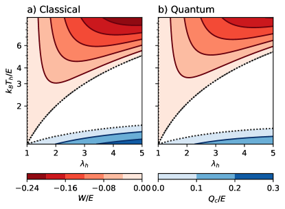
Figure 3: Energy output of an Otto cycle for the electric dipole machine setting with (a) a classical and (b) a quantum planar rotor. We plot against the hot-stroke control parameter $\lambda_{h}$ and temperature $T_{h}$, distinguishing between two operation modes marked by the dotted lines: Engine operation with work output $W<0$ (red shades) and refrigeration with heat output $Q_{c}>0$ (blue). The cold-stroke parameters are fixed at $k_{\mathrm{B}}T_{c}=E$ and $\lambda_{c}=1$.

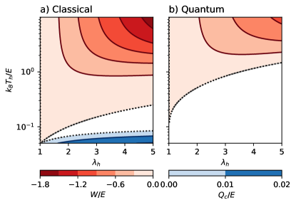
Figure 4: Energy output of (a) the classical and (b) the quantum electric dipole machine, plotted in the same manner as in Fig. 3 as a function of the hot-stroke control parameter $\lambda_{h}$ and temperature $T_{h}$. Here, we set the cold-stroke temperature to a lower value, $k_{\mathrm{B}}T_{c}=0.05E$.

IV Magnetic dipole machine

We now consider the setting of Fig. 1(b): a charged dumbbell or rod rotates in the $xy$-plane in the presence of a homogeneous magnetic field perpendicular to that plane, $\bm{B}_{\lambda}=B_{\lambda}\bm{e}_{z}$. Once again, the control parameter $\lambda$ determines the field strength. The charged rotor constitutes a circular current to which one can associate a magnetic dipole moment $\bm{\mu}=\mu L_{z}\bm{e}_{z}/\hbar$. Its potential energy in the field, $V=-\bm{\mu}\cdot\bm{B}_{\lambda}=-\omega_{\lambda}L_{z}$, can be given in terms of the controlled Larmor frequency $\omega_{\lambda}=\mu B_{\lambda}/\hbar\equiv\lambda\hbar/I$. The Hamiltonian of the so defined working medium is

$$H(\lambda)=\frac{L_{z}^{2}}{2I}-\omega_{\lambda}L_{z}=E\left[\frac{L_{z}^{2}}{2\hbar^{2}}-\lambda\frac{L_{z}}{\hbar}\right],$$ (18)

where $\hbar\lambda$ determines the net angular momentum displacement that minimizes the energy in the field.

IV.1 Classical no-go result

For a classical planar rotor, we will now show that the magnetic dipole configuration can neither operate as an Otto engine nor as a refrigerator, regardless of the chosen temperatures or control parameters.

The classical partition function of a Gibbs state is straightforwardly obtained after completing the square in the Hamiltonian (18),

$$Z(\lambda,T)=Z(0,T)\mathrm{e}^{E\lambda^{2}/2k_{\mathrm{B}}T}=2\pi\hbar\sqrt{\frac{2\pi k_{\mathrm{B}}T}{E}}\,\mathrm{e}^{E\lambda^{2}/2k_{\mathrm{B}}T}.$$ (19)

From this follow the relevant mean energies as

$$\langle H_{i}\rangle_{j} =\frac{\langle L_{z}^{2}\rangle_{j}}{2I}-\frac{E\lambda_{i}}{\hbar}\langle L_{z}\rangle_{j}$$

$$=k_{\mathrm{B}}T_{j}\left[T_{j}\frac{\partial}{\partial T_{j}}+(\lambda_{j}-\lambda_{i})\frac{\partial}{\partial\lambda_{j}}\right]\ln Z(\lambda_{j},T_{j})$$

$$=\frac{k_{\mathrm{B}}T_{j}}{2}+\frac{E\lambda_{j}}{2}(\lambda_{j}-2\lambda_{i}).$$ (20)

The resulting work and cold-bath heat input are

$$W =E(\lambda_{h}-\lambda_{c})\frac{\langle L_{z}\rangle_{h}-\langle L_{z}\rangle_{c}}{\hbar}$$

$$=E(\lambda_{h}-\lambda_{c})^{2}>0,$$ (21)

$$Q_{c} =\frac{\langle L_{z}^{2}\rangle_{c}-\langle L_{z}^{2}\rangle_{h}}{2I}-E\lambda_{c}\frac{\langle L_{z}\rangle_{c}-\langle L_{z}\rangle_{h}}{\hbar}$$

$$=-\frac{k_{\mathrm{B}}(T_{h}-T_{c})}{2}-\frac{E}{2}(\lambda_{h}-\lambda_{c})^{2}<0,$$ (22)

which precludes any useful operation of the Otto cycle.

IV.2 Quantum machine operation

We will now see that the quantum magnetic dipole setting allows for both an Otto engine and a refrigerator mode, provided that the cold strokes are operated close to the ground state. As before, the performance is determined by the characteristic mean energies $\langle H_{i}\rangle_{j}$, which can be given by derivatives of the partition function as in the second line of (20). The first lines in (21) and in (22) also hold, but with the expectation values taken over the quantum Gibbs state at $T_{h}$ and $T_{c}$. The associated partition function is a discrete sum due to angular momentum quantization. With help of the Poisson sum rule [57], we can express it as the product of the classical partition function (19) (in units of Planck’s action quantum) and a Jacobi theta function [58],

$$Z(\lambda,T) =\sum_{m=-\infty}^{+\infty}\mathrm{e}^{-Em(m-2\lambda)/2k_{\mathrm{B}}T}$$

$$=\sqrt{\frac{2\pi k_{\mathrm{B}}T}{E}}\,\mathrm{e}^{E\lambda^{2}/2k_{\mathrm{B}}T}\sum_{\nu=-\infty}^{+\infty}\!\mathrm{e}^{-2\pi\nu(i\lambda+\pi\nu k_{\mathrm{B}}T/E)}$$

$$=\sqrt{\frac{2\pi k_{\mathrm{B}}T}{E}}\,\mathrm{e}^{E\lambda^{2}/2k_{\mathrm{B}}T}\,\vartheta_{3}\left(-\pi\lambda,\mathrm{e}^{-2\pi^{2}k_{\mathrm{B}}T/E}\right).$$ (23)

The quantum expectation value of angular momentum, $\langle L_{z}\rangle=:\hbar(\lambda+\epsilon)$, can now deviate from the classical mean value $\hbar\lambda$ by at most $|\epsilon|<1/2$. In fact, we can invoke a functional identity of the Jacobi theta function to obtain an explicit Fourier expansion of the deviation [58],

$$\epsilon =\frac{\langle L_{z}\rangle}{\hbar}-\lambda=\frac{k_{\mathrm{B}}T}{E}\frac{\partial\ln Z(\lambda,T)}{\partial\lambda}-\lambda$$

$$=\sum_{n=1}^{\infty}(-)^{n}\frac{2\pi k_{\mathrm{B}}T/E}{\sinh(2\pi^{2}nk_{\mathrm{B}}T/E)}\sin(2\pi n\lambda).$$ (24)

Figure 5 plots the resulting $\langle L_{z}\rangle$ as a function of $\lambda$ for three temperatures of the underlying quantum Gibbs state. The deviation vanishes exactly for any $T$ whenever $\lambda$ assumes an integer or a half-integer value. Moreover, we observe that the quantum-classical deviation diminishes quickly with growing temperature $T$, and is here no longer visible at $k_{\mathrm{B}}T=0.5E$ (green line). In the opposite limit $k_{\mathrm{B}}T\ll E$ (blue curve), the Fourier-sine coefficients in (24) converge to $(-)^{n}/\pi n$, which describes a triangular sawtooth pattern and thus a stepwise increase of $\langle L_{z}\rangle=\hbar\ell$ at every half-integer $\lambda$.

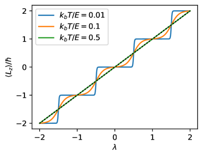
Figure 5: Mean angular momentum of a quantum planar rotor in Gibbs states of three different temperatures, with respect to the magnetic dipole Hamiltonian (18) of varying momentum displacement $\lambda$. The dotted line marks the classical mean value $\langle L_{z}\rangle=\hbar\lambda$, achieved at high temperatures.

To understand this behaviour, recall that the quantum Hamiltonian $\hat{H}(\lambda)$ is diagonal in the angular momentum basis $\{|m\rangle\}$. Its energy eigenvalues, $E_{m}=E(m-\lambda)^{2}/2-E\lambda^{2}/2$, are points on a parabola in $m$ that is centered around $\lambda$. For integer $\lambda$, we have one ground state at $m=\lambda$ and degenerate energy doublets at $m=\lambda\pm n$ with $n\in\mathbb{N}$. Assuming that these doublets are uniformly populated in thermal equilibrium (which would require the environment to induce incoherent transitions between them upon equilibration), we get $\langle L_{z}\rangle=\hbar\lambda$ regardless of temperature. Similarly, for half-integer $\lambda$, all energy states including the ground state are doubly degenerate with respect to $m=\lambda\pm(n-1/2)$, so that once again $\langle L_{z}\rangle=\hbar\lambda$. Deviations can only occur for $\lambda\mod 1/2\neq 0$. At low temperatures, the rotor then mainly occupies the angular momentum state $|\ell\rangle$ of minimal energy, with $\ell$ the integer closest to $\lambda$. Consequently, $\langle L_{z}\rangle\approx\hbar\ell=\hbar(\lambda+\epsilon)$ with deviation $|\epsilon|<\lambda\mod 1/2$.

Let us now discuss the implications of quantization for the engine operation regime. We shall restrict our view to the case $\lambda_{c}>\lambda_{h}$; the other case could be treated analogously. The per-cycle work in the first line of (21) can be rewritten as

$$W=E(\lambda_{c}-\lambda_{h})^{2}\left(1+\frac{\epsilon_{c}-\epsilon_{h}}{\lambda_{c}-\lambda_{h}}\right),$$ (25)

which must be negative (i.e., an output) for an engine. The fact that $|\epsilon_{c}\pm\epsilon_{h}|<1$ immediately restricts the choice of control parameters to $\lambda_{c}-\lambda_{h}<1$. Moreover, any integer offset of both parameter values, $\lambda_{h,c}\to\lambda_{h,c}+m$, is irrelevant, and the deviation $\epsilon$ is always negative (positive) for $\lambda$-values greater than (smaller than) the closest integer. This limits the engine regime to $0\leq\lambda_{h}<\lambda_{c}<1/2$, without loss of generality. The precise parameter window for $W<0$ also depends on the bath temperatures.

We have already seen that there is no work output in the classical regime of vanishing $\epsilon_{h,c}$, i.e., when both temperatures are high, $k_{\mathrm{B}}T_{h,c}>E$. In the opposite, deep quantum regime of $k_{\mathrm{B}}T_{h,c}\ll E$, we can approximate $W\approx E(\lambda_{c}-\lambda_{h})(\ell_{c}-\ell_{h})$, which is also non-negative due to the monotonicity of rounding to the closest integer. Appreciable work output only occurs in an intermediate regime of comparably low $T_{c}$ and comparably high $T_{h}$. Ideally, a cold stroke at vanishing temperature ($k_{\mathrm{B}}T_{c}\ll E$) and $\lambda_{c}$ close to $1/2$ should be combined with a hot stroke at high temperature ($k_{\mathrm{B}}T_{h}>E$), so that $\epsilon_{c}\approx-\lambda_{c}$ and $\epsilon_{h}\approx 0$. This achieves

$$\frac{W}{E}\approx-\left(\lambda_{c}-\lambda_{h}\right)\lambda_{h}=\left(\lambda_{h}-\frac{\lambda_{c}}{2}\right)^{2}-\frac{\lambda_{c}^{2}}{4}>-\frac{1}{16}.$$ (26)

In this case, setting $\lambda_{h}=\lambda_{c}/2$ results in the maximum work output of $E\lambda_{c}^{2}/4$ per cycle for a given $\lambda_{c}\in(0,1/2)$. Hence it is optimal to choose $\lambda_{c}$ as close as possible (but not identical) to $1/2$. The upper bound of $E/16$ work output can only be achieved asymptotically for $\lambda_{c}\to 1/2$ and $T_{c}\to 0$ .

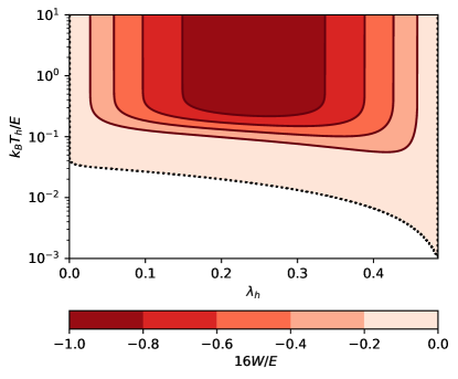
Figure 6: Energy output of an Otto cycle for the magnetic dipole machine setting with a quantum planar rotor. We plot against the hot-stroke control parameter $\lambda_{h}$ and temperature $T_{h}$, distinguishing between two operation modes marked by the dotted lines: engine operation with work output $W<0$ (red shades) and refrigeration with heat output $Q_{c}>0$ (blue). The cold-stroke parameters are fixed at $k_{\mathrm{B}}T_{c}=0.001E$ and $\lambda_{c}=0.485$. The Work output is normalized with respect to theoretically predicted optimum $W=-E/16$, see Equation (26).

The work output in the ideal engine regime is shown in Fig. 6 as a function of the hot-stroke parameters $\lambda_{h}$ and $T_{h}$ for fixed $\lambda_{c}=0.485$ and $k_{\mathrm{B}}T_{c}=0.001E$. We see that the work reaches close to the ideal value around $\lambda_{h}\approx 0.25$ and for temperatures $k_{\mathrm{B}}T_{h}>0.2E$.

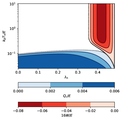
Figure 7: Energy output of the magnetic dipole machine, plotted in the same manner as Fig. 6 against the hot-stroke parameter $\lambda_{h}$ and the temperature $T_{h}$. The cold-stroke parameters are fixed at $k_{\mathrm{B}}T_{c}=0.025E$ and $\lambda_{c}=0.485$.

As one moves away from the ideal regime by increasing the cold temperature, the engine operation window closes and the work output deteriorates quickly. This is illustrated in Fig. 7, where we set $k_{\mathrm{B}}T_{c}=0.025E$. In this setting, we find that the Otto cycle can also operate as a refrigerator, provided that the hot temperature is small, $k_{\mathrm{B}}T_{h}<0.1E$. Overall, we have shown that, because of angular momentum quantization, the magnetic dipole machine supports useful operation modes in the low-temperature regime.

V Conclusion

We investigated two physically motivated realizations of an Otto cycle with a planar rotor as the working medium, highlighting differences in the operation regimes and performance due to quantization. The first realization consists of a rotating electric dipole subject to an electric field of controlled strength parallel to the rotation plane. The system thus resembles a mathematical pendulum. We found that angular momentum quantization leads to consistently lower energy output and smaller engine and fridge operation windows at low temperatures.

For the second realization, in which a charged rotor generates a magnetic moment subjected to a magnetic field of controlled strength, we showed that there is no useful output in the classical limit. For the quantized rotor, however, we could locate and characterise an engine operation mode in which the rotor state cycles between a deeply quantum cold temperature regime of almost no excitations and a quasi-classical hot regime of arbitrarily high excitations. This constitutes a genuinely quantum thermal machine model that differs from previously studied models based on few-level systems.

The discussed Otto machine models and their quantum features could be demonstrated in experiments with molecular rotors, levitated nanorotors, or with Josephson loops in circuit QED. Future work could explore the possibility of similar quantum features in other mechanical systems with a non-homogeneous energy spectrum.