An iterative method for the solution of Laplace-like
equations in high and very high space dimensions

Abstract

This paper deals with the equation $-\Delta u+\mu u=f$ on high-dimensional spaces $\mathbb{R}^{m}$, where the right-hand side $f(x)=F(Tx)$ is composed of a separable function $F$ with an integrable Fourier transform on a space of a dimension $n>m$ and a linear mapping given by a matrix $T$ of full rank and $\mu\geq 0$ is a constant. For example, the right-hand side can explicitly depend on differences $x_{i}-x_{j}$ of components of $x$. Following our publication [Numer. Math. (2020) 146:219–238], we show that the solution of this equation can be expanded into sums of functions of the same structure and develop in this framework an equally simple and fast iterative method for its computation. The method is based on the observation that in almost all cases and for large problem classes the expression $\|T^{t}y\|^{2}$ deviates on the unit sphere $\|y\|=1$ the less from its mean value the higher the dimension $m$ is, a concentration of measure effect. The higher the dimension $m$, the faster the iteration converges.

1 Introduction

The numerical solution of partial differential equations in high space dimensions is a difficult and challenging task. Methods such as finite elements, which work perfectly in two or three dimensions, are not suitable for solving such problems because the effort grows exponentially with the dimension. Random walk based techniques only provide solution values at selected points. Sparse grid methods are best suited for problems in still moderate dimensions. Tensor-based methods Bachmayr , Hackbusch_1 , Khoromskij stand out in this area. They are not subject to such limitations and perform surprisingly well in a large number of cases. Tensor-based methods exploit less the regularity of the solutions rather than their structure. Consider the equation

$$-\Delta u+\mu u=f$$ (1)

on $\mathbb{R}^{m}$ for high dimensions $m$, where $\mu>0$ is a given constant. Provided the right-hand side $f$ of the equation (1) possesses an integrable Fourier transform,

$$u(x)=\left(\frac{1}{\sqrt{2\pi}}\right)^{m}\!\int\frac{1}{\|\omega\|^{2}+\mu}\,\widehat{f}(\omega)\,\mathrm{e}^{\,\mathrm{i}\,\omega\cdot x}\,\mathrm{d}\omega$$ (2)

is a solution of this equation, and the only solution that tends uniformly to zero as $x$ goes to infinity. If the right-hand side $f$ of the equation is a tensor product

$$f(x)=\prod_{i}\phi_{i}(x_{i})$$ (3)

of functions, say from the three-dimensional space to the real numbers, or a sum of such tensor products, the same holds for the Fourier transform of $f$. If one replaces the corresponding term in the high-dimensional integral (2) by an approximation

$$\frac{1}{\|\omega\|^{2}+\mu}\approx\sum_{k}a_{k}\,\mathrm{e}^{-\beta_{k}\left(\|\omega\|^{2}+\mu\right)}=\sum_{k}a_{k}\,\mathrm{e}^{-\beta_{k}\mu}\prod_{i}\mathrm{e}^{-\beta_{k}\|\omega_{i}\|^{2}}$$ (4)

based on an appropriate approximation of $1/r$ by a sum of exponential functions, the integral then collapses to a sum of products of lower-dimensional integrals. That is, the solution can be approximated by a sum of such tensor products whose number is independent of the space dimension. The computational effort no longer increases exponentially, but only linearly with the space dimension.

However, the right-hand side of the equation does not always have such a simple structure and cannot always be well represented by tensors of low rank. A prominent example is quantum mechanics. The potential in the Schrödinger equation depends on the distances between the particles considered. Therefore, it is desirable to approximate the solutions of this equation by functions that explicitly depend on the position of the particles relative to each other. As a building block in more comprehensive calculations, this can require the solution of equations of the form (1) with right-hand sides that are composed of terms such as

$$f(x)=\bigg{(}\prod_{i}\phi_{i}(x_{i})\bigg{)}\bigg{(}\prod_{i<j}\phi_{ij}(x_{i}-x_{j})\bigg{)}.$$ (5)

The question is whether such structures transfer to the solution and whether in such a context arising iterates stay in this class. The present work deals with this problem. We present a conceptually simple iterative method that preserves such structures and takes advantage of the high dimensions.

First we embed the problem as in our former paper Yserentant_2020 into a higher dimensional space introducing, for example, some or all differences $x_{i}-x_{j}$, $i<j$, in addition to the components $x_{i}$ of the vector $x\in\mathbb{R}^{m}$ as additional variables. We assume that the right-hand side of the equation (1) is of the form $f(x)=F(Tx)$, where $T$ is a matrix of full rank that maps the vectors in $\mathbb{R}^{m}$ to vectors in an $\mathbb{R}^{n}$ of a still higher dimension and $F:\mathbb{R}^{n}\to\mathbb{R}$ is a function that possesses an integrable Fourier transform and as such is continuous. The solution of the equation (1) is then the trace $u(x)=U(Tx)$ of the then equally continuous function

$$U(y)=\left(\frac{1}{\sqrt{2\pi}}\right)^{n}\!\int\frac{1}{\|T^{t}\omega\|^{2}+\mu}\,\widehat{F}(\omega)\,\mathrm{e}^{\,\mathrm{i}\,\omega\cdot y}\,\mathrm{d}\omega,$$ (6)

which is, in a corresponding sense, the solution of a degenerate elliptic equation

$$\mathcal{L}U+\mu U=F.$$ (7)

This equation replaces the original equation (1). Its solution (6) is approximated by the iterates arising from a polynomially accelerated version of the basic method

$$U_{k+1}=\,U_{k}\,-\,(-\Delta+\mu)^{-1}(\mathcal{L}U_{k}+\mu U_{k}-F).$$ (8)

The calculation of these iterates requires the solution of equations of the form (1), that is, the calculation of integrals of the form (2), now not over $\mathbb{R}^{m}$, but over the higher dimensional $\mathbb{R}^{n}$. The symbol $\|T^{t}\omega\|^{2}$ of the operator $\mathcal{L}$ is a homogeneous second-order polynomial in $\omega$. For separable right-hand sides $F$ as above, the calculation of these integrals thus reduces to the calculation of products of lower, in the extreme case one-dimensional integrals.

The reason for the usually astonishingly good approximation properties of these iterates is the directional behavior of the term $\|T^{t}\omega\|^{2}$, more precisely the fact that the euclidean norm of the vectors $T^{t}\eta\in\mathbb{R}^{m}$ for vectors $\eta$ on the unit sphere $S^{n-1}$ of the $\mathbb{R}^{n}$ takes an almost constant value outside a very small set whose size decreases rapidly with increasing dimensions, a typical concentration of measure effect. To capture this phenomenon quantitatively, we introduce the probability measure

$$\mathbb{P}(M)=\frac{1}{n\nu_{n}}\int_{M\cap S^{n-1}}\!\,\mathrm{d}\eta$$ (9)

on the Borel subsets $M$ of the $\mathbb{R}^{n}$, where $\nu_{n}$ is the volume of the unit ball and $n\nu_{n}$ thus is the area of the unit sphere. If $M$ is a subset of the unit sphere, $\mathbb{P}(M)$ is equal to the ratio of the area of M to the area of the unit sphere. If $M$ is a sector, that is, if $M$ contains with a vector $\omega$ also its scalar multiples, $\mathbb{P}(M)$ measures the opening angle of $M$. In the following we assume that the mean value of the expression $\|T^{t}\eta\|^{2}$ over the unit sphere, or in other words its expected value with respect to the given probability measure, takes the value one. This is only a matter of the scaling of the variables in the higher dimensional space and does not represent a restriction. The decisive quantity is the variance of the expression $\|T^{t}\eta\|^{2}$, considered as a random variable on the unit sphere. Since the values $\|T^{t}\eta\|^{2}$ are, except for rather extreme cases, approximately normally distributed in higher dimensions, the knowledge of the variance makes it possible to capture the distribution of these values sufficiently well. The concentration of measure effect is reflected in the fact that the variances almost always tend to zero as the dimensions increase.

For a given $\rho<1$, let $S$ be the sector that consists of the points $\omega$ for which the expression $\|T^{t}\omega\|^{2}$ differs from $\|\omega\|^{2}$ by $\rho\|\omega\|^{2}$ or less. If the Fourier transform of the right-hand side of the equation (7) vanishes at all $\omega$ outside this set, the same holds for the Fourier transform of its solution (6) and the Fourier transforms of the iterates $U_{k}$. Under this condition, the iteration error decreases at least like

$$\|U-U_{k}\|\leq\rho^{k}\|U\|$$ (10)

with respect to a broad range of Fourier-based norms. Provided the values $\|T^{t}\eta\|^{2}$ are approximately normally distributed with expected value $E=1$ and small variance $V$, the measure (9) of the sector $S$ is almost one as soon as $\rho$ exceeds the standard deviation $\sigma=\sqrt{V}$ by more than a moderate factor. The sector $S$ then fills almost the entire frequency space. This is admittedly an idealized situation and the actual convergence behavior is more complicated, but this example characterizes pretty well what one can expect. The higher the dimensions and the smaller the variance, the faster the iterates approach the solution.

The rest of this paper is organized as follows. Section 2 sets the framework and is devoted to the representation of the solutions of the equation (1) as traces of higher dimensional functions (6) for right-hand sides that are themselves traces of functions with an integrable Fourier transform. In comparison with the proof in Yserentant_2020 , we give a more direct proof of this representation. In addition, we introduce two scales of norms with respect to which we later estimate the iteration error.

In a sense, the following two sections form the core of the present work. They deal with the distribution of the values $\|T^{t}\eta\|^{2}$ on the unit sphere. Section 3 treats the general case. We first show that the expected value $E$ and the variance $V$ of the expression $\|T^{t}\eta\|^{2}$, considered as a random variable, can be expressed in terms of the singular values of the matrix $T$. Using this representation, we show that for random matrices $T$ with assigned expected value $E=1$ the expected value of the corresponding variances $V$ not only tends to zero as the dimension $m$ goes to infinity, but also that these variances cluster the more around their expected value the larger $m$ is. Sampling large numbers of these variances supports these theoretical findings. We also study a class of matrices $T$ that are associated with interaction graphs. These matrices correspond to the case that some or all coordinate differences are introduced as additional variables and formed the original motivation for this work. The expected values $E$ that are assigned to these matrices always take the value one and the corresponding variances $V$ can be expressed directly in terms of the vertex degrees and the dimensions. Numerical experiments for standard classes of random graphs show that the variances tend to zero with high probability as the number of the vertices increases. As mentioned, the knowledge of the expected value and the variance assigned to a given matrix $T$ is of central importance since the distribution of the values $\|T^{t}\eta\|^{2}$ is usually not much different from the corresponding normal distribution. This can be checked experimentally by sampling these values for a large number of uniformly distributed points $\eta$ on the unit sphere.

These observations are supported by the results for orthogonal projections from a higher onto a lower dimensional space presented in Sect. 4, a case which is accessible to a complete analysis and that for this reason serves us as a model problem. These results are based on a precise knowledge of the corresponding probability distributions and are related to the random projection theorem and the Johnson-Lindenstrauss lemma Vershynin . This section is based in some parts on results from our former papers Yserentant_2020 and Yserentant_2022 , which are taken up here and are adapted to the present situation.

In Sect. 5 we finally return to the higher-dimensional counterpart (7) of the original equation (1) and study the convergence behavior of the polynomially accelerated version of the iteration (8) for its solution. Special attention is given to the limit case $\mu=0$ of the Laplace equation. The section ends with a brief review of an approximation of the form (4) by sums of Gauss functions.

2 Solutions as traces of higher-dimensional functions

In this paper we are mainly concerned with functions $U:\mathbb{R}^{n}\to\mathbb{R}$, $n$ a potentially high dimension, that possess the then unique representation

$$U(y)=\left(\frac{1}{\sqrt{2\pi}}\right)^{n}\!\int\widehat{U}(\omega)\,\mathrm{e}^{\,\mathrm{i}\,\omega\cdot y}\,\mathrm{d}\omega$$ (1)

in terms of an integrable function $\widehat{U}$, their Fourier transform. Such functions are uniformly continuous by the Riemann-Lebesgue theorem and vanish at infinity. The space $\mathcal{B}_{0}(\mathbb{R}^{n})$ of these functions becomes a Banach space under the norm

$$\|U\|=\left(\frac{1}{\sqrt{2\pi}}\right)^{n}\!\int|\widehat{U}(\omega)|\,\mathrm{d}\omega.$$ (2)

Let $T$ be an arbitrary $(n\times m)$-matrix of full rank $m<n$ and let

$$u:\mathbb{R}^{m}\to\mathbb{R}:x\to U(Tx)$$ (3)

be the trace of a function in $U\in\mathcal{B}_{0}(\mathbb{R}^{n})$. Since the functions in $\mathcal{B}_{0}(\mathbb{R}^{n})$ are uniformly continuous, the same also applies to the traces of these functions. Since there is a constant $c$ with $\|x\|\leq c\,\|Tx\|$ for all $x\in\mathbb{R}^{m}$, the trace functions (3) vanish at infinity as $U$ itself. The next lemma gives a criterion for the existence of partial derivatives of the trace functions, where we use the common multi-index notation.

Lemma 1

Let $U:\mathbb{R}^{n}\to\mathbb{R}$ be a function in $\mathcal{B}_{0}(\mathbb{R}^{n})$ and let the functions

$$\omega\to(\mathrm{i}\,T^{t}\omega)^{\beta}\widehat{U}(\omega),\quad\beta\leq\alpha,$$ (4)

be integrable. Then the trace function (3) possesses the partial derivative

$$(\mathrm{D}^{\alpha}u)(x)=\left(\frac{1}{\sqrt{2\pi}}\right)^{n}\!\int(\mathrm{i}\,T^{t}\omega)^{\alpha}\widehat{U}(\omega)\,\mathrm{e}^{\,\mathrm{i}\,\omega\cdot Tx}\,\mathrm{d}\omega,$$ (5)

which is, like $u$, itself uniformly continuous and vanishes at infinity.

Proof

Let $e_{k}\in\mathbb{R}^{m}$ be the vector with the components $e_{k}|_{j}=\delta_{kj}$. To begin with, we examine the limit behavior of the difference quotient

$$\frac{u(x+he_{k})-u(x)}{h}=\left(\frac{1}{\sqrt{2\pi}}\right)^{n}\!\int\frac{\mathrm{e}^{\,\mathrm{i}\,h\omega\cdot Te_{k}}-1}{h}\;\widehat{U}(\omega)\,\mathrm{e}^{\,\mathrm{i}\,\omega\cdot Tx}\,\mathrm{d}\omega$$

of the trace function as $h$ goes to zero. Because of

$$\left|\,\frac{\mathrm{e}^{\,\mathrm{i}\,ht}-1}{h}\,\right|\leq\,|\,t\,|,\quad\lim_{h\to 0}\frac{\mathrm{e}^{\,\mathrm{i}\,ht}-1}{h}=\,\mathrm{i}\,t,$$

and under the condition that the function $\omega\to\omega\cdot Te_{k}\,\widehat{U}(\omega)$ is integrable, it tends to

$$(\mathrm{D}_{k}u)(x)=\left(\frac{1}{\sqrt{2\pi}}\right)^{n}\!\int\mathrm{i}\,\omega\cdot Te_{k}\,\widehat{U}(\omega)\,\mathrm{e}^{\,\mathrm{i}\,\omega\cdot Tx}\,\mathrm{d}\omega$$

as follows from the dominated convergence theorem. Because of $\omega\cdot Te_{k}=T^{t}\omega\cdot e_{k}$, this proves (5) for partial derivatives of order one. For partial derivatives of higher order, the proposition follows by induction. ∎

Let $D(\mathcal{L})$ be the space of the functions $U\in\mathcal{B}_{0}(\mathbb{R}^{n})$ with finite (semi)-norm

$$|\,U|_{T}=\left(\frac{1}{\sqrt{2\pi}}\right)^{n}\!\int\|T^{t}\omega\|^{2}\,|\widehat{U}(\omega)|\,\mathrm{d}\omega.$$ (6)

Because of $|(T^{t}\omega)^{\beta}|\leq 1+\|T^{t}\omega\|^{2}$ for all multi-indices $\beta$ of order two or less, the traces of the functions in this space are twice continuously differentiable by Lemma 1. Let $\mathcal{L}:D(\mathcal{L})\to\mathcal{B}_{0}(\mathbb{R}^{n})$ be the pseudo-differential operator given by

$$(\mathcal{L}U)(y)=\left(\frac{1}{\sqrt{2\pi}}\right)^{n}\!\int\|T^{t}\omega\|^{2}\,\widehat{U}(\omega)\,\mathrm{e}^{\,\mathrm{i}\,\omega\cdot y}\,\mathrm{d}\omega.$$ (7)

For the functions $U\in D(\mathcal{L})$ and their traces (3), by Lemma 1

$$-\,(\Delta u)(x)=(\mathcal{L}U)(Tx)$$ (8)

holds. With corresponding right-hand sides, the solutions of the equation (1) are thus the traces of the solutions $U\in D(\mathcal{L})$ of the pseudo-differential equation

$$\mathcal{L}U+\mu U=F.$$ (9)

Theorem 2.1

Let $F:\mathbb{R}^{n}\to\mathbb{R}$ be a function with integrable Fourier transform, let $f(x)=F(Tx)$, and let $\mu$ be a positive constant. Then the trace (3) of the function

$$U(y)=\left(\frac{1}{\sqrt{2\pi}}\right)^{n}\!\int\frac{1}{\|T^{t}\omega\|^{2}+\mu}\,\widehat{F}(\omega)\,\mathrm{e}^{\,\mathrm{i}\,\omega\cdot y}\,\mathrm{d}\omega$$ (10)

is twice continuously differentiable and the only solution of the equation

$$-\Delta u+\mu u=f$$ (11)

whose values tend uniformly to zero as $\|x\|$ goes to infinity. Provided the function

$$\omega\,\to\,\frac{1}{\|T^{t}\omega\|^{2}}\,\widehat{F}(\omega)\,$$ (12)

is integrable, the same holds in the limit case $\mu=0$.

Proof

That the trace $u$ is a classical solution of the equation (11) follows from the remarks above, and that $u$ vanishes at infinity by the already discussed reasons from the Riemann-Lebesgue theorem. The maximum principle ensures that no further solution of the equation (11) exists that vanishes at infinity. ∎

From now on, the equation (9) will replace the original equation (11). Our aim is to compute its solution (10) iteratively by polynomial accelerated versions of the basic iteration (8). The convergence properties of this iteration depend decisively on the directional behavior of the values $\|T^{t}\omega\|^{2}$, which will be studied in the next two sections, before we return to the equation and its iterative solution.

Before we continue with these considerations and turn our attention to the directional behavior of these values, we introduce the norms with respect to which we will show convergence. The starting point is the radial-angular decomposition

$$\int_{\mathbb{R}^{n}}f(x)\,\mathrm{d}x\,=\int_{S^{n-1}}\bigg{(}\int_{0}^{\infty}\!f(r\eta)r^{n-1}\,\mathrm{d}r\bigg{)}\,\mathrm{d}\eta$$ (13)

of the integrals of functions in $L_{1}(\mathbb{R}^{n})$ into an inner radial and an outer angular part. Inserting the characteristic function of the unit ball, one recognizes that the area of the $n$-dimensional unit sphere $S^{n-1}$ is $n\nu_{n}$, with $\nu_{n}$ the volume of the unit ball. If $f$ is rotationally symmetric, $f(r\eta)=f(re)$ holds for every $\eta\in S^{n-1}$ and every fixed, arbitrarily given unit vector $e$. In this case, (13) simplifies to

$$\int f(x)\,\mathrm{d}x\,=\,n\nu_{n}\int_{0}^{\infty}\!f(re)r^{n-1}\,\mathrm{d}r.$$ (14)

The norms split into two groups, both of which depend on a smoothness parameter. The norms in the first group possess the radial-angular representation

$$\|U\|_{s}=\frac{1}{n\nu_{n}}\int_{S^{n-1}}\bigg{(}n\nu_{n}\int_{0}^{\infty}|\widehat{U}(r\eta)|\,r^{s+n-1}\,\mathrm{d}r\bigg{)}\,\mathrm{d}\eta$$ (15)

and take in cartesian coordinates the more familiar form

$$\|U\|_{s}=\int_{\mathbb{R}^{n}}|\widehat{U}(\omega)|\|\omega\|^{s}\,\mathrm{d}\omega.$$ (16)

The spectral Barron spaces $\mathcal{B}_{s}=\mathcal{B}_{s}(\mathbb{R}^{n})$, $s\geq 0$, consist of the functions $U$ with finite norms $\|U\|_{t}$ for $0\leq t\leq s$. Since all these norms scale differently, we do not combine them to an entity but treat them separately. One should be aware that these norms are quite strong. For integer values $s$, functions $U\in\mathcal{B}_{s}$ possess continuous partial derivatives up to order $s$, which are bounded by the norms $\|U\|_{k}$, $k\leq s$, and vanish at infinity. Barron spaces play a prominent role in the analysis of neural networks and in high-dimensional approximation theory in general; see for example Siegel-Xu .

The norms in the second group are a mixture between an $L_{1}$-based norm, in radial direction, and an $L_{2}$-based norm for the angular part and are given by

$$|\!|\!|U|\!|\!|_{s}^{2}=\frac{1}{n\nu_{n}}\int_{S^{n-1}}\bigg{(}n\nu_{n}\int_{0}^{\infty}|\widehat{U}(r\eta)|\,r^{s+n-1}\,\mathrm{d}r\bigg{)}^{2}\,\mathrm{d}\eta.$$ (17)

If the norm $|\!|\!|U|\!|\!|_{s}$ of $U$ is finite, then also the norm $\|U\|_{s}$ and

$$\|U\|_{s}\leq|\!|\!|U|\!|\!|_{s}$$ (18)

holds. This follows from the Cauchy-Schwarz inequality. Both norms scale in the same way. By (14), they coincide for radially symmetric functions.

The following lemma is needed to bring these two norms into connection with Theorem 2.1 and the solution (10) of the equation (9).

Lemma 2

Let $m\geq 3$ and $m\geq 5$, respectively. Then the surface integrals

$$\frac{1}{n\nu_{n}}\int_{S^{n-1}}\!\frac{1}{\|T^{t}\eta\|^{2}}\,\mathrm{d}\eta,\quad\frac{1}{n\nu_{n}}\int_{S^{n-1}}\!\frac{1}{\|T^{t}\eta\|^{4}}\,\mathrm{d}\eta$$ (19)

take finite values, despite the singular integrands.

Proof

Let $\Sigma_{0}$ be the $(m\times m)$-diagonal matrix with the singular values of $T$ on its diagonal. A variable transform and the Fubini-Tonelli theorem then lead to

$$\int_{\mathbb{R}^{n}}\frac{1}{\|T^{t}\omega\|^{2}}\,\mathrm{e}^{-\|\omega\|^{2}}\!\,\mathrm{d}\omega\;=\int_{\mathbb{R}^{m}}\frac{1}{\|\Sigma_{0}\omega_{1}\|^{2}}\,\mathrm{e}^{-\|\omega_{1}\|^{2}}\!\,\mathrm{d}\omega_{1}\int_{\mathbb{R}^{n-m}}\!\mathrm{e}^{-\|\omega_{2}\|^{2}}\!\,\mathrm{d}\omega_{2}.$$

Because the first of the two integrals on the right-hand side of this identity is finite for dimensions $m\geq 3$ and the second without such a constraint, the integral

$$\int_{\mathbb{R}^{n}}\frac{1}{\|T^{t}\omega\|^{2}}\,\mathrm{e}^{-\|\omega\|^{2}}\!\,\mathrm{d}\omega\;=\frac{1}{n\nu_{n}}\int_{S^{n-1}}\!\frac{1}{\|T^{t}\eta\|^{2}}\,\mathrm{d}\eta\;\int_{0}^{\infty}\frac{1}{r^{2}}\,\mathrm{e}^{-r^{2}}r^{n-1}\,\mathrm{d}r$$

takes a finite value. The same then also holds for the integral over the unit sphere on the right-hand side of the equation. For dimensions $m\geq 5$, the second of the two integrals in (19) can be treated in the same way. ∎

For a given function $F$ with integrable Fourier transform, the function

$$\widehat{U}(\omega)=\frac{1}{\|T^{t}\omega\|^{2}}\,\widehat{F}(\omega)$$ (20)

possesses the radial-angular representation

$$\widehat{U}(r\eta)=\frac{1}{\|T^{t}\eta\|^{2}}\,\frac{\widehat{F}(r\eta)}{r^{2}}.$$ (21)

If the function $\phi:S^{n-1}\to\mathbb{R}$ given by

$$\phi(\eta)=n\nu_{n}\int_{S^{n-1}}\bigg{|}\frac{\widehat{F}(r\eta)}{r^{2}}\bigg{|}\,r^{n-1}\,\mathrm{d}r$$ (22)

is bounded and the dimension $m$ is three or higher, the function (20) is integrable by Lemma 2 and Fourier transform of a function $U\in\mathcal{B}_{0}(\mathbb{R}^{n})$ with finite norm $\|U\|_{0}$. For dimensions $m$ greater than four, it suffices that $\phi$ is square integrable. For the other norms introduced above, one can argue in a similar way.

3 A moment-based analysis

The purpose of this and the next section is to study how much the pseudo-differential operator (7) differs from the negative Laplace operator, that is, how much

$$\chi(\omega)=\|T^{t}\omega\|^{2}$$ (1)

deviates on the unit sphere $S^{n-1}$ of the $\mathbb{R}^{n}$ from the constant one. The expression (1) is a homogeneous function of second order in the variable $\omega$. To study its angular distribution, we make use of the already introduced probability measure

$$\mathbb{P}(M)=\frac{1}{n\nu_{n}}\int_{M\cap S^{n-1}}\!\,\mathrm{d}\eta$$ (2)

on the Borel subsets $M$ of the $\mathbb{R}^{n}$. The direct calculation of the expected values of the given and other homogeneous functions as surface integrals is complicated. We therefore reduce the calculation of such quantities to the calculation of simpler volume integrals. Our main tool is the radial-angular decomposition (13).

Lemma 3

Let $x\to\|x\|^{2\ell}\,W(x)$ be rotationally symmetric and integrable. Then

$$\frac{1}{n\nu_{n}}\int_{S^{n-1}}\chi(\eta)\,\mathrm{d}\eta=\,C(\ell)\int_{\mathbb{R}^{n}}\chi(x)W(x)\,\mathrm{d}x$$ (3)

holds for all functions $\chi$ that are positively homogeneous of degree $2\ell\geq 0$, where the constant $C(\ell)$ is given by the expression

$$\frac{1}{C(\ell)}=\,n\nu_{n}\int_{0}^{\infty}\!W(re)r^{2\ell+n-1}\,\mathrm{d}r$$ (4)

and $e$ is an arbitrarily given unit vector.

Proof

As by assumption $\chi(r\eta)=r^{2\ell}\chi(\eta)$ and $W(r\eta)=W(re)$ holds for $\eta\in S^{n-1}$ and $r>0$, the decomposition (13) leads to

$$\int_{\mathbb{R}^{n}}\chi(x)W(x)\,\mathrm{d}x\,=\int_{S^{n-1}}\chi(\eta)\left(\int_{0}^{\infty}\!r^{2\ell}\,W(re)r^{n-1}\,\mathrm{d}r\right)\!\,\mathrm{d}\eta,$$

yielding the proposition after some rearrangement. ∎

The choice of the function $W$ can be adapted to the needs. For example, it can be the characteristic function of the unit ball or the normed Gauss function

$$W(x)=\left(\frac{1}{\sqrt{\pi}}\right)^{n}\exp\big{(}-\|x\|^{2}\big{)},$$ (5)

which breaks down into a product of univariate functions. Another almost trivial, but often very useful observation concerns coordinate changes.

Lemma 4

Under the assumptions from the previous lemma,

$$\int_{\mathbb{R}^{n}}\chi(x)W(x)\,\mathrm{d}x=\int_{\mathbb{R}^{n}}\chi(Qx)W(x)\,\mathrm{d}x$$ (6)

holds for all orthogonal $(n\times n)$-matrices $Q$.

Proof

The transformation theorem for multivariate integrals leads to

$$\int_{\mathbb{R}^{n}}\chi(x)W(x)\,\mathrm{d}x=\int_{\mathbb{R}^{n}}\chi(Qx)W(Qx)|\mathrm{det}Q|\,\mathrm{d}x.$$

Because $W(Qx)=W(x)$ and $\mathrm{det}Q=\pm 1$, the proposition follows. ∎

The expected value and the variance of the function (1), the central moments

$$E=\frac{1}{n\nu_{n}}\int_{S^{n-1}}\!\|T^{t}\eta\|^{2}\,\mathrm{d}\eta,\quad V=\frac{1}{n\nu_{n}}\int_{S^{n-1}}\!\big{(}\|T^{t}\eta\|^{2}-E\big{)}^{2}\,\mathrm{d}\eta,$$ (7)

are of fundamental importance for our considerations.

Lemma 5

The expected value and the variance of the function (1) depend only on the singular values $\sigma_{1},\ldots,\sigma_{m}$ of the matrix $T$. In terms of the power sums

$$A_{1}=\sum_{i=1}^{m}\sigma_{i}^{2},\quad A_{2}=\sum_{i=1}^{m}\sigma_{i}^{4}$$ (8)

of order one and two of the squares of the singular values, they read as follows

$$E=\frac{A_{1}}{n},\quad V=\frac{2n\,A_{2}-2A_{1}^{2}}{n^{2}(n+2)}.$$ (9)

Proof

Inserting the matrix $Q$ from the singular value decomposition $T=Q\Sigma\widetilde{Q}^{t}$ of the matrix $T$, Lemma 3 and Lemma 4 lead to the representation

$$\frac{1}{n\nu_{n}}\int_{S^{n-1}}\big{(}\|T^{t}\eta\|^{2})^{k}\,\mathrm{d}\eta=C(k)\int_{\mathbb{R}^{n}}\bigg{(}\sum_{i=1}^{m}\!\sigma_{i}^{2}x_{i}^{2}\bigg{)}^{k}W(x)\,\mathrm{d}x$$

of the moment of order $k$ as a homogeneous symmetric polynomial in the $\sigma_{i}^{2}$. With the function $W$ from (5), the volume integral on the right-hand side splits into a sum of products of one-dimensional integrals. Using

$$\int_{0}^{\infty}t^{j}\mathrm{e}^{-t^{2}}\,\mathrm{d}t=\frac{1}{2}\,\Gamma\left(\frac{j+1}{2}\right),\;\;\nu_{n}=\frac{2}{n}\,\frac{\pi^{n/2}}{\Gamma(n/2)},$$

this integral and the constant $C(k)$ can be calculated in principle. For the first two moments, this is easily possible. For moments of order three and higher, one can take advantage of the fact that the symmetric polynomials are polynomials in the power sums of the $\sigma_{i}^{2}$; see VanDerWarden , or Sturmfels for a more recent treatment. ∎

In terms of the normalized singular values $\eta_{i}=\sigma_{i}/\sqrt{n}$, the expected value and the variance (7) and (9), respectively, can be written as follows

$$E=\sum_{i=1}^{m}\eta_{i}^{2},\quad V=\frac{2n}{n+2}\,\sum_{i=1}^{m}\eta_{i}^{4}\,-\,\frac{2}{n+2}\,\bigg{(}\sum_{i=1}^{m}\eta_{i}^{2}\bigg{)}^{2}.$$ (10)

We are interested in matrices $T$ for which the expected value $E$ is one, that is, for which the vector $\eta$ composed of the normalized singular values $\eta_{i}$ lies on the unit sphere of the $\mathbb{R}^{m}$. The variances $V$ then possess the representation

$$V=\frac{2n}{n+2}\,X(\eta)\,-\,\frac{2}{n+2},\quad X(\eta)=\sum_{i=1}^{m}\eta_{i}^{4}.$$ (11)

The function $X$ attains the minimum value $1/m$ and the maximum value one on the unit sphere of the $\mathbb{R}^{m}$. The variances (11) therefore extend over the interval

$$\frac{n-m}{n+2}\,\frac{2}{m}\leq V<\frac{2n-2}{n+2}$$ (12)

and can be arbitrarily close to the value two for large $n$. The spectral norms of the given matrices $T^{t}$, their maximum singular values $\sigma_{i}$, spread over the interval

$$\sqrt{\frac{n}{m}}\leq\|T^{t}\|<\sqrt{n}.$$ (13)

However, the variances are most likely of the order $\mathcal{O}(1/m)$.

Lemma 6

Let the vectors $\eta$ composed of the normalized singular values $\eta_{i}$ be uniformly distributed on the part of the unit sphere consisting of points with strictly positive components. Then the expected value and the variance of $X$ are

$$\mathbb{E}(X)=\frac{3}{m+2},\quad\mathbb{V}(X)=\frac{24m-24}{(m+2)^{2}(m+4)(m+6)}.$$ (14)

Proof

For symmetry reasons and because the intersections of lower-dimensional subspaces with the unit sphere have measure zero, we can allow points $\eta$ that are uniformly distributed on the whole unit sphere. The expected value and the variance of the function $X$, treated as a random variable, are therefore

$$\mathbb{E}(X)=\frac{1}{m\nu_{m}}\int_{S^{m-1}}X(\eta)\,\mathrm{d}\eta,\quad\mathbb{V}(X)=\frac{1}{m\nu_{m}}\int_{S^{m-1}}\big{(}X(\eta)-\mathbb{E}(X)\big{)}^{2}\,\mathrm{d}\eta$$

and can be calculated along the lines given by Lemma 3. ∎

It is instructive to express the variance (11) in terms of the random variable

$$\widetilde{X}(\eta)=\frac{m+2}{3}\,X(\eta),$$ (15)

which is rescaled to the expected value $\mathbb{E}(\widetilde{X})=1$. Its variance

$$\mathbb{V}(\widetilde{X})=\frac{8}{3}\,\frac{m-1}{(m+4)(m+6)}$$ (16)

tends to zero as $m$ goes to infinity. This not only means that the expected value

$$V^{*}=\,\frac{2n}{n+2}\,\frac{3}{m+2}\,-\,\frac{2}{n+2}$$ (17)

of the variances $V$ tends to zero as the dimension $m$ increases, but also that the variances cluster the more around their expected value the larger $m$ is. This observation is supported by simple, easily reproducible experiments. Uniformly distributed points on the unit sphere $S^{m-1}$ can be generated from vectors in $\mathbb{R}^{m}$ with components that are subject to the standard normal distribution. Such vectors then follow themselves the standard normal distribution in the $m$-dimensional space. Scaling them to length one gives the desired uniformly distributed points on the unit sphere. This allows one to sample the random variable $X$ for any given dimension $m$.

The expected value and the variance (7) can be expressed directly in terms of the entries of the $(m\times m)$-matrix $S=T^{t}T$, since the power sums (8) are the traces

$$A_{1}=\sum_{i=1}^{m}S_{ii},\quad A_{2}=\sum_{i,j=1}^{m}S_{ij}^{2}$$ (18)

of the matrices $S$ and $S^{2}$, and can therefore be computed without recourse to the singular values of $T$. Consider the $(n\times m)$-matrix $T$ assigned to an arbitrarily given undirected graph with $m$ vertices and $n-m$ edges that maps the components $x_{i}$ of a vector $x\in\mathbb{R}^{m}$ first to themselves and then to the $n-m$ weighted differences

$$\frac{x_{i}-x_{j}}{\sqrt{2}},\quad i<j,$$ (19)

assigned to the edges of the graph connecting the vertices $i$ and $j$. In quantum physics, matrices of the given kind can be associated with the interaction of particles. They formed the original motivation for this work. In the given case, the matrix $S$ has the form $S=I+L/2$, where $I$ is the identity matrix and $L$ is the Laplacian matrix of the graph. The off-diagonal entries of $L$ are $L_{ij}=-1$ if the vertices $i$ and $j$ are connected by an edge and $L_{ij}=0$ otherwise. The diagonal entries $L_{ii}=d_{i}$ are the vertex degrees, the numbers of edges that meet at the vertices $i$.

Lemma 7

For a matrix $T$ of dimension $n\times m$ associated with a graph with $m$ vertices and $n-m$ edges, the expected value and the variance (7) are

$$E=1,\quad V=\left(\frac{d^{2}-6}{2}\,\frac{m}{n}\,+\,3\right)\frac{1}{n+2},$$ (20)

where the quantity $d^{2}$ is the mean value of the squares of the vertex degrees:

$$d^{2}=\frac{1}{m}\sum_{i=1}^{m}d_{i}^{2}.$$ (21)

Proof

By (18), the constants (8) possess the representation

$$A_{1}=n,\quad A_{2}=\frac{d^{2}-6}{4}\,m\,+\,\frac{5}{2}\,n$$

in the case considered here. The proposition therefore follows from (9). ∎

If the squares of the vertex degrees remain bounded in the mean, the variance tends to zero inversely proportional to the total number of vertices and edges. The matrices assigned to graphs whose vertices up to one are connected with a designated central vertex, but not to each other, form the other extreme. For these matrices, the variances decrease to a limit value greater than zero as the number of vertices increases. However, such matrices are a very rare exception, not only with respect to the above random matrices, but also in the context of matrices assigned to graphs. Consider the random graphs with a fixed number $m$ of vertices that are with a given probability $p$ connected by an edge, or those with a fixed number $m$ of vertices and $n-m$ of edges. Sampling the variances assigned to a large number of graphs in such a class, one sees that these variances exceed the value $2/(m+1)$ with a very high probability at most by a factor that is only slightly greater than one, if at all. If all vertices are connected with each other, if their degree is $d_{i}=m-1$ and the number of edges is therefore $n-m=m(m-1)/2$, the variance is

$$V=\frac{m^{2}+m-2}{m^{2}+m+4}\frac{2}{m+1}.$$ (22)

With the exception of a few extreme cases, it can be observed that the distribution of the values $\|T^{t}\eta\|^{2}$ for points $\eta$ on the unit sphere of $\mathbb{R}^{n}$ more and more approaches the normal distribution with the expected value and the variance (7) as the dimensions increase, a fact that underlines the importance of these quantities. This can be seen by evaluating the expression $\|T^{t}\eta\|^{2}$ at a large number of independently chosen, uniformly distributed points $\eta$ on the unit sphere and comparing the frequency distribution of the resulting values with the given Gauss function

$$\frac{1}{\sqrt{2\pi V}}\,\exp\left(-\,\frac{(x-E)^{2}}{2V}\,\right).$$ (23)

Let the matrix $T$ have the singular value decomposition $T=Q\Sigma\widetilde{Q}^{t}$. The frequency distribution of the values $\|\Sigma^{t}\eta\|^{2}=\|T^{t}Q\eta\|^{2}$ on the unit sphere then coincides with the distribution of the values $\|T^{t}\eta\|^{2}$. Let $\Sigma_{0}$ be the $(m\times m)$-diagonal matrix that is composed of the singular values. Given the above remarks about the generation of uniformly distributed points on a unit sphere, sampling the values $\|T^{t}\eta\|^{2}$ for a large number of points $\eta\in S^{n-1}$ means to sample the ratio

$$\frac{\|\Sigma_{0}x\|^{2}}{\|x\|^{2}+\|y\|^{2}}$$ (24)

for a large number of vectors $x\in\mathbb{R}^{m}$ and $y\in\mathbb{R}^{n-m}$ with standard normally distributed components. The values $\|y\|^{2}$ are then distributed according to the $\chi^{2}$-distribution with $n-m$ degrees of freedom. The direct calculation of $\|y\|^{2}$ can thus be replaced by the calculation of a single scalar quantity following this distribution. The amount of work then remains strictly proportional to the dimension $m$, no matter how large the difference $n-m$ of the dimensions is. Let $T$ be the matrix assigned to the graph associated with the $\mathrm{C}_{60}$-fullerene molecule, which consists of of the ninety edges of a truncated icosahedron and its sixty corners as vertices. The degree of these vertices is three and the assigned variance therefore $V=9/380$. The frequency distribution of the values $\|T^{t}\eta\|^{2}$ for a million randomly chosen points $\eta$ on the unit sphere and the corresponding Gauss function (23) are shown in Fig. 1.

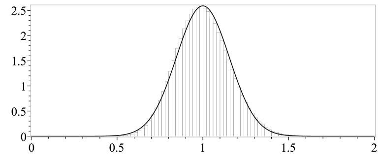
Figure 1: The frequency distribution of the values $\|T^{t}\eta\|^{2}$ for the matrix $T$ associated with the $\mathrm{C}_{60}$-molecule

The singular values of the matrices $T$ and $T^{t}$, respectively, can in general only be determined numerically. The matrices $T$ assigned to complete graphs, in which all vertices are connected with each other, are an exception. It is not difficult to see that the associated matrices $S=T^{t}T$ have the eigenvalue one of multiplicity one and the eigenvalue $(m+2)/2$ of multiplicity $m-1$ in terms of the number $m$ of vertices. The square roots of these eigenvalues are the singular values of $T$.

Orthogonal projections, matrices $T^{t}=P$ of dimension $(m\times n)$ with one as the only singular value, are another important exception. The quantities (8) take the value $m$ in this case. The expected value and the variance are therefore

$$E=\frac{m}{n},\quad V=\frac{m}{n}\left(1-\frac{m}{n}\right)\frac{2}{n+2},$$ (25)

or after rescaling, that is, after multiplying $P$ by the factor $\sqrt{n/m}$,

$$E=1,\quad V=\frac{n-m}{n+2}\,\frac{2}{m}.$$ (26)

Since $\|\Sigma_{0}x\|^{2}=\|x\|^{2}$ for orthogonal projections, for these matrices the quotient (24) follows the beta distribution with the probability density function

$$f(t)=\frac{\Gamma(\alpha+\beta)}{\Gamma(\alpha)\Gamma(\beta)}\;t^{\alpha-1}(1-t)^{\beta-1}$$ (27)

with parameters $\alpha=m/2$ and $\beta=(n-m)/2$; see (Abramowitz-Stegun, , Eq. 26.5.3). In a context similar to ours, this has already been observed in Frankl-Maehara . Orthogonal projections are accessible to a complete analysis. The next section is therefore devoted to their study.

4 Orthogonal projections and measure concentration

We begin with a simple, but very helpful corollary from Lemma 4.

Lemma 8

Let $A$ be an arbitrary matrix of dimension $m\times n$, $m<n$, with singular value decomposition $A=Q\Sigma\widetilde{Q}^{t}$. Then the probabilities

$$\mathbb{P}\big{(}\big{\{}x\,\big{|}\,\|Ax\|^{2}\leq\delta\|A\|^{2}\|x\|^{2}\big{\}}\big{)},\quad\mathbb{P}\big{(}\big{\{}x\,\big{|}\,\|\Sigma x\|^{2}\leq\delta\|\Sigma\|^{2}\|x\|^{2}\big{\}}\big{)}$$ (1)

are equal and the first one depends only on the singular values of $A$.

Proof

This follows from the invariance of these probabilities under orthogonal transformations. Let $\chi(x)=1$ if $\|Ax\|^{2}\leq\delta\|A\|^{2}\|x\|^{2}$ holds and $\chi(x)=0$ otherwise. The transformed function, with the values $\chi(\widetilde{Q}x)$, is then the characteristic function of the set of all $x$ for which $\|\Sigma x\|^{2}\leq\delta\|\Sigma\|^{2}\|x\|^{2}$ holds. ∎

The next theorem is an only slightly modified version of Theorem 2.4 in Yserentant_2022 . Its proof is based on the observation that the probability (1) is equal to the volume of the set of all $x$ inside the unit ball for which $\|Ax\|^{2}\leq\delta\|A\|^{2}\|x\|^{2}$ holds, up to the division by the volume of the unit ball itself. This is an implication of Lemma 3 if the characteristic function of the unit ball is chosen as the function $W$.

Theorem 4.1

Let the $(m\times n)$-matrix $P$ be an orthogonal projection. Then

$$\mathbb{P}\big{(}\big{\{}x\,\big{|}\,\|Px\|^{2}\leq\delta\|x\|^{2}\big{\}}\big{)}=F(\delta),\quad 0\leq\delta<1,$$ (2)

holds, where the function $F(\delta)=F(m,n;\delta)$ is defined by the integral expression

$$F(\delta)=\frac{\Gamma(\alpha+\beta)}{\Gamma(\alpha)\Gamma(\beta)}\,\int_{0}^{\delta}t^{\alpha-1}(1-t)^{\beta-1}\,\mathrm{d}t$$ (3)

and the two exponents $\alpha$ and $\beta$ are given by

$$\alpha=\frac{m}{2},\quad\beta=\frac{n-m}{2}.$$ (4)

The function (2) tends to the limit value $F(1)=1$ as $\delta$ goes to one.

Proof

By Lemma 8, we can restrict ourselves to the matrix $P$, which extracts from a vector in $\mathbb{R}^{n}$ its first $m$ components. We split the vectors in $\mathbb{R}^{n}$ into a part $x\in\mathbb{R}^{m}$ and a remaining part $y\in\mathbb{R}^{n-m}$. The set whose volume has to be calculated according to the above remark, then consists of the points in the unit ball for which

$$\|x\|^{2}\leq\delta\big{(}\,\|x\|^{2}+\|y\|^{2}\,\big{)}$$

or, resolved for the norm of the component $x\in\mathbb{R}^{m}$,

$$\|x\|\leq\varepsilon\,\|y\|,\quad\varepsilon=\sqrt{\frac{\delta}{1-\delta}}\,,$$

holds. This volume can be expressed as double integral

$$\int\left(\int H\big{(}\varepsilon\|y\|-\|x\|\big{)}\chi\big{(}\|x\|^{2}+\|y\|^{2}\big{)}\,\mathrm{d}x\right)\!\,\mathrm{d}y,$$

where $H(t)=0$ for $t<0$, $H(t)=1$ for $t\geq 0$, $\chi(t)=1$ for $t\leq 1$, and $\chi(t)=0$ for arguments $t>1$. If $\delta$ tends to one and $\varepsilon$ thus to infinity, the value of this double integral tends, by the dominated convergence theorem, to the volume of the unit ball and the expression (2) tends to one, as claimed. In terms of polar coordinates, that is, according to (14), the double integral is given by

$$(n-m)\nu_{n-m}\int_{0}^{\infty}\left(m\nu_{m}\int_{0}^{\varepsilon s}\chi\big{(}r^{2}+s^{2}\big{)}r^{m-1}\,\mathrm{d}r\right)s^{n-m-1}\,\mathrm{d}s,$$

where $\nu_{d}$ is the volume of the unit ball in $\mathbb{R}^{d}$. By substituting $t=r/s$ in the inner integral, the upper bound becomes independent of $s$ and the integral simplifies to

$$(n-m)\nu_{n-m}\int_{0}^{\infty}\left(m\nu_{m}\,s^{m}\!\int_{0}^{\varepsilon}\chi\big{(}s^{2}(1+t^{2})\big{)}t^{m-1}\,\mathrm{d}t\right)s^{n-m-1}\,\mathrm{d}s.$$

Interchanging the order of integration, it attains the value

$$\frac{(n-m)\nu_{n-m}\,m\nu_{m}}{n}\int_{0}^{\varepsilon}\frac{t^{m-1}}{(1+t^{2})^{n/2}}\,\mathrm{d}t.$$

With $\varphi(t)=t^{2}/(1+t^{2})$ and the constants $\alpha$ and $\beta$ from (4), one obtains

$$\int_{0}^{\varepsilon}\frac{t^{m-1}}{(1+t^{2})^{n/2}}\,\mathrm{d}t=\frac{1}{2}\int_{0}^{\varepsilon}\varphi(t)^{\alpha-1}(1-\varphi(t))^{\beta-1}\varphi^{\prime}(t)\,\mathrm{d}t$$

and, because of $\varphi(0)=0$ and $\varphi(\varepsilon)=\delta$, therefore the representation

$$\int_{0}^{\varepsilon}\frac{t^{m-1}}{(1+t^{2})^{n/2}}\,\mathrm{d}t=\frac{1}{2}\int_{0}^{\delta}t^{\alpha-1}(1-t)^{\beta-1}\,\mathrm{d}t$$

of the integral. Dividing the expression above by $\nu_{n}$ and recalling that

$$\nu_{d}=\frac{2}{d}\,\frac{\pi^{d/2}}{\Gamma(d/2)},$$

this completes the proof of the theorem. ∎

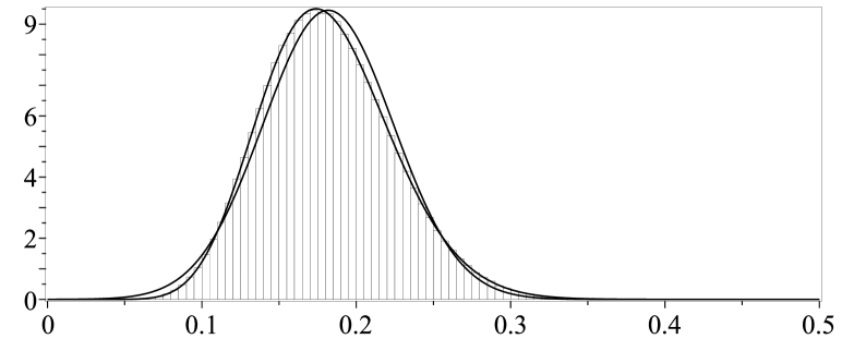
Figure 2: The frequency distribution of the values $\|Px\|^{2}$ for the dimensions $m=30$ and $n=165$ together with the exact distribution from Theorem 4.1 and its approximation by the Gauss function (23)

That is, for points $x$ on the unit sphere, the values $\|Px\|^{2}$ follow the beta distribution mentioned at the end of the last section. For smaller dimensions, the frequency distribution $f(t)=F^{\prime}(t)$ and its approximation by the Gauss function (23) still differ considerably, as can be seen in Fig. 2. This difference vanishes with increasing dimensions. In fact, it is common knowledge in statistics that beta distributions behave in the limit of large parameters almost like normal distributions. If a random variable $X(\omega)$ with expected value $E$ and standard deviation $\sigma$ follows a beta distribution with parameters $\alpha$ and $\beta$, the distribution of the random variable

$$\frac{X(\omega)-E}{\sigma}$$ (5)

differs the less from the standard normal distribution as $\alpha$ and $\beta$ become larger. For the sake of completeness, we prove this in the following. Let

$$B(\alpha,\beta;x)=\frac{\Gamma(\alpha+\beta)}{\Gamma(\alpha)\Gamma(\beta)}\int_{0}^{x}t^{\alpha-1}(1-t)^{\beta-1}\,\mathrm{d}t$$ (6)

be the distribution function of the beta distribution with parameters $\alpha$ and $\beta$, let $E$ and $V$ be the assigned expected value and the assigned variance given by

$$E=\frac{\alpha}{\alpha+\beta},\quad V=\frac{\alpha\beta}{(\alpha+\beta)^{2}(\alpha+\beta+1)},$$ (7)

and let $\sigma=\sqrt{V}$ be the corresponding standard deviation. The function (6) is first only defined for arguments $0\leq x\leq 1$. To avoid problems with its domain of definition, we extend it by the value zero for arguments $x<0$ and the value one for arguments $x>1$. If $\alpha$ and $\beta$ are greater than one, which is the only us interesting case, the extended function is a continuously differentiable cumulative distribution function with a density that vanishes outside the interval $0<t<1$. Let

$$\widetilde{B}(\alpha,\beta;x)=B(\alpha,\beta;\sigma x+E)$$ (8)

be the accordingly rescaled distribution function.

Theorem 4.2

The function (8) tends pointwise to the distribution function

$$\Phi(x)=\frac{1}{\sqrt{2\pi}}\int_{-\infty}^{x}\mathrm{e}^{-t^{2}/2}\,\mathrm{d}t.$$ (9)

of the standard normal distribution as $\alpha$ and $\beta$ go to infinity.

Proof

Before we start with the proof itself, we recall that it suffices to show that the assigned densities converge pointwise to the density of the normal distribution. This may be surprising in view of the monotone or the dominated convergence theorem, but is easily explained and is often utilized in stochastics. Let $f_{1},f_{2},\ldots$ be a sequence of densities that converges pointwise to a density $f$. The nonnegative functions

$$h_{n}(x)=\inf_{k\geq n}f_{k}(x)$$

then tend pointwise monotonously from below to $f$ and it is

$$\int_{-\infty}^{x}\!h_{n}(t)\,\mathrm{d}t\,\leq\,\int_{-\infty}^{x}\!f_{n}(t)\,\mathrm{d}t\,\leq\,1\,-\int_{x}^{\infty}\!h_{n}(t)\,\mathrm{d}t,$$

where we have used that the integral of $f_{n}$ over $\mathbb{R}$ takes the value one. The two outer integrals converge, by the monotone convergence theorem, to the limits

$$\int_{-\infty}^{x}\!f(t)\,\mathrm{d}t,\quad\int_{x}^{\infty}\!f(t)\,\mathrm{d}t\,=\,1\,-\int_{-\infty}^{x}\!f(t)\,\mathrm{d}t.$$

This proves that the middle integral converges to the limit

$$\lim_{n\to\infty}\,\int_{-\infty}^{x}\!f_{n}(t)\,\mathrm{d}t\,=\int_{-\infty}^{x}\!f(t)\,\mathrm{d}t.$$

Pointwise convergence of the densities thus implies convergence in distribution.

Now let us fix an arbitrary finite interval and assume that the parameters $\alpha$ and $\beta$ are already so large that, for the points $x$ in this interval, the quantities

$$\bigg{(}\frac{\sigma}{E}\,x\bigg{)}^{2}\!=\,\frac{1}{\alpha}\frac{\beta x^{2}}{\alpha+\beta+1},\quad\bigg{(}\frac{\sigma}{1-E}\,x\bigg{)}^{2}\!=\,\frac{1}{\beta}\,\frac{\alpha x^{2}}{\alpha+\beta+1}$$

take values less than $9/100$. On the given interval, the density of the distribution (8), its derivative with respect to the variable $x$, can then be written as follows

$$\frac{\Gamma(\alpha+\beta)(E+\sigma x)^{\alpha-1}(1-E-\sigma x)^{\beta-1}\sigma}{\Gamma(\alpha)\Gamma(\beta)}.$$

To proceed, we need Stirling’s formula (see (DLMF, , Eq. 5.6.1)), the representation

$$\Gamma(z)=\sqrt{2\pi}\,z^{z-1/2}\mathrm{e}^{-z}\,\mathrm{e}^{\mu(z)},\quad 0<\mu(z)<\frac{1}{12z},$$

of the gamma function for real arguments $z>0$. Introducing the function

$$g(z)=\ln(\sqrt{2\pi})+\bigg{(}z-\frac{1}{2}\bigg{)}\ln(z)-z,$$

the logarithm of the density breaks down into the sum of the three terms

$$A=\ln(\sigma)+g(\alpha+\beta)-g(\alpha)-g(\beta)+(\alpha-1)\ln(E)+(\beta-1)\ln(1-E),$$

$$B=(\alpha-1)\ln\bigg{(}1+\frac{\sigma}{E}\,x\bigg{)}+(\beta-1)\ln\bigg{(}1-\frac{\sigma}{1-E}\,x\bigg{)},$$

$$C=\mu(\alpha+\beta)-\mu(\alpha)-\mu(\beta).$$

The third term $C$ tends by definition to zero as $\alpha$ and $\beta$ go to infinity. The first of the three terms can be easily calculated and reduces to the value

$$A=\ln\bigg{(}\frac{1}{\sqrt{2\pi}}\bigg{)}+\frac{1}{2}\ln\bigg{(}\frac{\alpha+\beta}{\alpha+\beta+1}\bigg{)}.$$

By means of the second-order Taylor expansion

$$\ln(1+t)=P(t)+R(t),\quad P(t)=t-\frac{1}{2}\,t^{2},$$

of $\ln(1+t)$ around $t=0$, the second term splits into the polynomial part

$$B_{1}=(\alpha-1)P\bigg{(}\frac{\sigma}{E}\,x\bigg{)}+(\beta-1)P\bigg{(}\!-\frac{\sigma}{1-E}\,x\bigg{)}$$

and a remainder $B_{2}$. The polynomial part possesses the representation

$$B_{1}={}-\frac{1-a}{2}\,x^{2}+bx,$$

with coefficients $a$ and $b$ that depend on the parameters $\alpha$ and $\beta$ and are given by

$$a\,=\frac{1}{\alpha}\,\frac{\beta}{\alpha+\beta+1}+\frac{1}{\alpha+\beta+1}+\frac{1}{\beta}\,\frac{\alpha}{\alpha+\beta+1},$$

$$\;b\,=\bigg{(}\frac{1}{\beta}\,\frac{\alpha}{\alpha+\beta+1}\bigg{)}^{1/2}\!\!-\;\bigg{(}\frac{1}{\alpha}\,\frac{\beta}{\alpha+\beta+1}\bigg{)}^{1/2}.$$

Because of $|R(t)|\leq|t|^{3}$ for $|t|\leq 3/10$ and our assumption about the size of $\alpha$ and $\beta$ in dependence of the interval under consideration, the term $B_{2}$ can be estimated as

$$|B_{2}|\leq(\alpha-1)\bigg{(}\frac{x^{2}}{\alpha}\bigg{)}^{3/2}\!\!+\;(\beta-1)\bigg{(}\frac{x^{2}}{\beta}\bigg{)}^{3/2}.$$

The logarithm of the density tends on the given interval therefore uniformly to

$$\ln\bigg{(}\frac{1}{\sqrt{2\pi}}\bigg{)}-\,\frac{1}{2}\,x^{2}$$

as $\alpha$ and $\beta$ go to infinity. This implies locally uniform convergence of the densities themselves and thus at least pointwise convergence of the distributions ∎

However, the key message of this section remains that the values $\|Px\|^{2}$ cluster, for points $x$ on the unit sphere, more and more around their expected value $\xi=m/n$ as the dimensions increase. Much better than by the previous theorem this is reflected by the following result, which again is more or less taken from Yserentant_2022 . A similar technique, based in the same way on the Markov inequality, was used in Dasgupta-Gupta . The following estimates are expressed in terms of the function

$$\phi(\vartheta)=\sqrt{\vartheta}\,\exp\left(\frac{1-\vartheta}{2}\right).$$ (10)

It increases strictly on the interval $0\leq\vartheta\leq 1$, reaches its maximum value one at the point $\vartheta=1$, and decreases strictly from there.

Theorem 4.3

Let the $(m\times n)$-matrix $P$ be an orthogonal projection and let $\xi$ be ratio of the two dimensions $m$ and $n$. For $0<\delta<\xi$, then

$$\mathbb{P}\big{(}\big{\{}x\,\big{|}\,\|Px\|^{2}\leq\delta\,\|x\|^{2}\big{\}}\big{)}\leq\,\phi\left(\frac{\delta}{\xi}\right)^{m}\phantom{.}$$ (11)

holds. For $\xi<\delta<1$, this estimate is complemented by the estimate

$$\mathbb{P}\big{(}\big{\{}x\,\big{|}\,\|Px\|^{2}>\delta\,\|x\|^{2}\big{\}}\big{)}\leq\,\phi\left(\frac{\delta}{\xi}\right)^{m}.$$ (12)

Proof

As before, we can restrict ourselves to the matrix $P$ that extracts from a vector in $\mathbb{R}^{n}$ its first $m$ components. The characteristic function $\chi$ of the set of all $x$ for which the estimate $\|Px\|^{2}\leq\delta\,\|x\|^{2}$ holds satisfies, for all $t>0$, the estimate

$$\chi(x)\leq\exp\big{(}\,t\,\big{(}\delta\|x\|^{2}-\|Px\|^{2}\big{)}\big{)}$$

by a product of univariate functions. Choosing the normed weight function (5), the left-hand side of (11) can, by Lemma 3, therefore be estimated by the integral

$$\left(\frac{1}{\sqrt{\pi}}\right)^{n}\!\int\exp\big{(}\,t\,\big{(}\delta\|x\|^{2}-\|Px\|^{2}\big{)}\big{)}\exp\big{(}-\|x\|^{2}\big{)}\,\mathrm{d}x,$$

which remains finite for all $t$ in the interval $0\leq t<1/\delta$. It splits into a product of one-dimensional integrals and takes, for given $t$, the value

$$\left(\frac{1}{1-\delta t+t}\right)^{m/2}\left(\frac{1}{1-\delta t}\right)^{(n-m)/2}.$$

This expression attains its minimum on the interval $0<t<1/\delta$ at

$$t=\frac{\xi-\delta}{(1-\delta)\delta}.$$

At this point $t$ it takes the value

$$\left(\left(\frac{\delta}{\xi}\right)^{1/2}\!\left(\frac{1-\delta}{1-\xi}\right)^{\gamma}\;\right)^{m},\quad\gamma=\frac{1-\xi}{2\xi}.$$

With the abbreviation $\delta/\xi=\vartheta$ and because of $\vartheta\xi<1$ and $\xi<1$, the logarithm

$$\ln\left(\left(\frac{1-\delta}{1-\xi}\right)^{\gamma}\;\right)=\,\frac{1-\xi}{\xi}\,\ln\left(\frac{1-\vartheta\xi}{1-\xi}\right)$$

possesses the power series expansion

$$\frac{1-\vartheta}{2}-\frac{1}{2}\,\sum_{k=1}^{\infty}\left(\frac{1-\vartheta^{k}}{k}-\,\frac{1-\vartheta^{k+1}}{k+1}\right)\xi^{k}.$$

Because the series coefficients are for all $\vartheta\geq 0$ greater than or equal to zero and, by the way, polynomial multiples of $(1-\vartheta)^{2}$, the estimate (11) follows.

The proof of the second estimate is almost identical to the proof of the first. For sufficiently small $t>0$, the expression (12) can be estimated by the integral

$$\left(\frac{1}{\sqrt{\pi}}\right)^{n}\!\int\exp\big{(}\,t\,\big{(}\|Px\|^{2}-\delta\|x\|^{2}\big{)}\big{)}\exp\big{(}-\|x\|^{2}\big{)}\,\mathrm{d}x.$$

This integral splits into a product of one-dimensional integrals and takes the value

$$\left(\frac{1}{1+\delta t-t}\right)^{m/2}\left(\frac{1}{1+\delta t}\right)^{(n-m)/2},$$

which attains, for $\delta<1$, on the interval $0<t<1/(1-\delta)$ its minimum at

$$t=\frac{\delta-\xi}{(1-\delta)\delta}.$$

At this point $t$ it again takes the value

$$\left(\left(\frac{\delta}{\xi}\right)^{1/2}\!\left(\frac{1-\delta}{1-\xi}\right)^{\gamma}\;\right)^{m},\quad\gamma=\frac{1-\xi}{2\xi}.$$

This leads, as above, to the estimate (12). ∎

If the dimension ratio $\xi=m/n$ is fixed or only tends to a limit value $\delta_{0}$, then the probability distributions (2) and the functions (3), respectively, tend to a step function with jump discontinuity at $\delta_{0}$. Figure 3 reflects this behavior. One can look at the estimates from Theorem 4.3 also from a different perspective and consider the rescaled counterparts $P^{\prime}=\sqrt{n/m}\,P$ of the projections $P$. The distributions

$$\mathbb{P}\big{(}\big{\{}x\,\big{|}\,\|P^{\prime}x\|^{2}\leq\delta\|x\|^{2}\big{\}}\big{)}$$ (13)

assigned to them tend, outside every small neighborhood of $\delta_{0}=1$, exponentially to a step function with jump discontinuity at $\delta_{0}=1$ as $m$ goes to infinity, independent of the ratio $m/n$ of the two dimensions, no matter how small it may be.

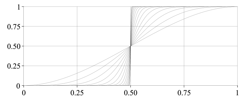
Figure 3: The probability distributions (2) as function of $0\leq\delta<1$ for $m=2^{k}$, $k=1,\ldots,16$, and $n=2m$

5 The iterative procedure

Now we are ready to analyze the iterative method

$$U_{0}=0,\quad U_{k+1}=\,U_{k}\,-\,(-\Delta+\mu)^{-1}(\mathcal{L}U_{k}+\mu U_{k}-F)$$ (1)

presented in the introduction and its polynomially accelerated counterpart, respectively, for the solution of the equation (9), the equation that has replaced the original equation (1). The iteration error possesses the Fourier representation

$$(\widehat{U}-\widehat{U}_{k})(\omega)=P_{k}\big{(}\alpha(\omega)(\|T^{t}\omega\|^{2}+\mu)\big{)}\widehat{U}(\omega),$$ (2)

where $U$ is the exact solution (10) of the equation (9), $\alpha(\omega)$ is given by

$$\alpha(\omega)=\frac{1}{\|\omega\|^{2}+\mu},$$ (3)

and the functions $P_{k}(\lambda)$ are polynomials of order $k$ with value $P_{k}(0)=1$. Throughout this section, we assume that the expression $\|T^{t}\eta\|^{2}$ possesses the expected value one. We restrict ourselves to the analysis of this iteration in the spectral Barron spaces $\mathcal{B}_{s}$ equipped with the norm (16), or (15) in radial-angular representation. In a corresponding sense, this analysis can be transferred to the Hilbert spaces $H^{s}$.

Theorem 5.1

If the solution $U$ lies in the Barron space $\mathcal{B}_{s}(\mathbb{R}^{n})$, $s\geq 0$, this also holds for the iterates $U_{k}$. For all coefficients $\mu\geq 0$, the norm (16) of the error, given by

$$\|U-U_{k}\|_{s}=\int\big{|}P_{k}\big{(}\alpha(\omega)(\|T^{t}\omega\|^{2}+\mu)\big{)}\widehat{U}(\omega)\big{|}\|\omega\|^{s}\,\mathrm{d}\omega,$$ (4)

then tends to zero for suitably chosen polynomials $P_{k}$ as $k$ goes to infinity.

Proof

Because the expression $\|T^{t}\eta\|^{2}$ possesses the expected value one, the spectral norm of the matrix $T^{t}$ attains a value $\|T^{t}\|\geq 1$. If one sets $\vartheta=1/\|T^{t}\|^{2}$,

$$0\leq 1-\vartheta\alpha(\omega)(\|T^{t}\omega\|^{2}+\mu)<1$$

therefore holds for all $\omega$ outside the kernel of $T^{t}$, as a subspace of a dimension less than $n$ a set of measure zero. Choosing $P_{k}(\lambda)=(1-\vartheta\lambda)^{k}$, the proposition thus follows from the dominated convergence theorem. ∎

Of course, one would like to have more than just convergence. The next theorem is a first step in this direction.

Theorem 5.2

Let $0<\rho<1$, $a=1-\rho$, $b=\|T^{t}\|^{2}$, and $\kappa=b/a$ and let

$$P_{k}(\lambda)=T_{k}\bigg{(}\dfrac{b+a-2\lambda}{b-a}\bigg{)}\bigg{/}T_{k}\bigg{(}\dfrac{b+a}{b-a}\bigg{)}$$ (5)

be the to the interval $\alpha\leq\lambda\leq b$ transformed Chebyshev polynomial $T_{k}$ of the first kind of degree $k$. The norm (16) of the iteration error (2) then satisfies the estimate

$$\|U_{k}-U\|_{s}\leq\frac{2r^{k}}{1+2r^{2k}}\,\|U\|_{s}+\|U-U_{\rho}\|_{s},\quad r=\frac{\sqrt{\kappa}-1}{\sqrt{\kappa}+1},$$ (6)

where $\widehat{U}_{\rho}$ takes the same values as $\widehat{U}$ on the set of all $\omega$ for which

$$1-\rho\leq\alpha(\omega)(\|T^{t}\omega\|^{2}+\mu)$$ (7)

holds and vanishes outside this set.

Proof

This follows from $0\leq\alpha(\omega)(\|T^{t}\omega\|^{2}+\mu)\leq b$ for $\omega\in\mathbb{R}^{n}$ and the estimates

$$|P_{k}(\lambda)|\leq 1\text{\;for $0\leq\lambda\leq a$},\quad|P_{k}(\lambda)|\leq\frac{2r^{k}}{1+2r^{2k}}\text{\;for $a\leq\lambda\leq b$}$$

for the values of the Chebyshev polynomial (5) on the interval $0\leq\lambda\leq b$. ∎

Depending on the size of $\kappa=\|T^{t}\|^{2}/(1-\rho)$, the norm of the error $U-U_{k}$ soon reaches the size of the norm of $U-U_{\rho}$. The idea behind the estimate (6) is that in high space dimensions the condition (7) is satisfied for nearly all $\omega$ and that the part $U-U_{\rho}$ of $U$ is therefore often negligible. The set on which the condition (7) is violated is a subset of the sector

$$S(\delta)=\big{\{}\omega\,\big{|}\|T^{t}\omega\|^{2}\leq\delta\|\omega\|^{2}\big{\}}$$ (8)

for $\delta=1-\rho$. Let the expression $\|T^{t}\omega\|^{2}$ possess the angular distribution

$$\mathbb{P}(S(\delta))=\int_{-\infty}^{\delta}f(t)\,\mathrm{d}t.$$ (9)

Consider the solution $U$ of the equation (9) for a rotationally symmetric right-hand side $F$ with finite norm $\|F\|_{s}$, and let $\chi(t)=1$ for $t\leq\delta$ and $\chi(t)=0$ for $t>\delta$. Then

$$\int_{S(\delta)}|\widehat{U}(\omega)|\|\omega\|^{s+2}\,\mathrm{d}\omega\,\leq\frac{1}{n\nu_{n}}\int_{S^{n-1}}\frac{\chi\big{(}\|T^{t}\eta\|^{2}\big{)}}{\|T^{t}\eta\|^{2}}\,\mathrm{d}\eta\,\|F\|_{s}$$ (10)

holds, independent of $\mu$ and with equality for $\mu=0$. This follows from the radial-angular representation of the involved integrals. By Lemma 2, the integral over the unit sphere on the right-hand side has a finite value for dimensions $m\geq 3$. In terms of the distribution density from (9), it is given by

$$\frac{1}{n\nu_{n}}\int_{S^{n-1}}\frac{\chi\big{(}\|T^{t}\eta\|^{2}\big{)}}{\|T^{t}\eta\|^{2}}\,\mathrm{d}\eta\,=\int_{0}^{\delta}\frac{f(t)}{t}\,\mathrm{d}t$$ (11)

and tends to zero as $\delta$ goes to zero, for higher dimensions usually very rapidly as the example of the (rescaled) orthogonal projections from Theorem 4.1 shows.

The estimate (6) is extremely robust in many respects. First, it is based on a pointwise estimate of the Fourier transform of the error. It is therefore equally valid for other Fourier-based norms. Second, the function (3) can be replaced by any approximation $\widetilde{\alpha}(\omega)$ for which an estimate

$$0\leq\widetilde{\alpha}(\omega)\leq(1+\varepsilon)\alpha(\omega)$$ (12)

on the entire frequency space and an inverse estimate

$$(1-\varepsilon)\alpha(\omega)\leq\widetilde{\alpha}(\omega)$$ (13)

on a sufficiently large ball around the origin hold without losing too much. This applies in particular to approximations by sums of Gauss functions.

Nevertheless, the estimate from Theorem 5.2 is rather pessimistic, because it only takes into account the decay of the left tail of the distribution (9), but ignores the fast decay of its right tail. To see what can be reached, we study the behavior of the iteration in the limit $\mu=0$, the case where the underlying effects are most clearly brought to light. Decomposing the vectors $\omega=r\eta$ into a radial part $r\geq 0$ and an angular part $\eta\in S^{n-1}$, the error (2) propagates frequency-wise as

$$(\widehat{U}-\widehat{U}_{k})(r\eta)=P_{k}\bigg{(}\frac{r^{2}\|T^{t}\eta\|^{2}+\mu}{r^{2}+\mu}\bigg{)}\widehat{U}(r\eta),$$ (14)

and after the transition to the limit value $\mu=0$ as

$$(\widehat{U}-\widehat{U}_{k})(r\eta)=P_{k}\big{(}\|T^{t}\eta\|^{2}\big{)}\widehat{U}(r\eta).$$ (15)

In the limit case, therefore, the method acts only on the angular part of the error. Nevertheless, by Theorem 5.1 the iterates converge to the solution. To clarify the underlying effects, we prove this once again in a different form.

Theorem 5.3

If the solution $U$ lies in the Barron space $\mathcal{B}_{s}(\mathbb{R}^{n})$, $s\geq 0$, this also holds for the iterates $U_{k}$ implicitly given by (15). The norm (15) of the iteration error then tends to zero for suitably chosen polynomials $P_{k}$ as $k$ goes to infinity.

Proof

In radial-angular representation, the iteration error is given by

$$\|U-U_{k}\|_{s}=\frac{1}{n\nu_{n}}\int_{S^{n-1}}\big{|}P_{k}\big{(}\|T^{t}\eta\|^{2}\big{)}\big{|}\phi(\eta)\,\mathrm{d}\eta,$$

where the integrable function $\phi:S^{n-1}\to\mathbb{R}$ is defined by the expression

$$\phi(\eta)\,=\,n\nu_{n}\int_{0}^{\infty}|\widehat{U}(r\eta)|\,r^{s+n-1}\,\mathrm{d}r.$$

To prove the convergence of the iterates $U_{k}$ to the solution $U$, we again consider the polynomials $P_{k}(t)=(1-\vartheta t)^{k}$ with $\vartheta=1/\|T^{t}\|^{2}$. For $\eta\in S^{n-1}$, it is

$$0\leq 1-\vartheta\|T^{t}\eta\|^{2}\leq 1,$$

where the value one is only attained on the intersection of the $(n-m)$-dimensional kernel of the matrix $T^{t}$ with the unit sphere, that is, on a set of area measure zero. The convergence again follows from the dominated convergence theorem. ∎

Under a seemingly harmless additional assumption, one gets a rather sharp, hardly to improve estimate for the speed of convergence.

Theorem 5.4

Under the assumption that the norm given by (17) of the solution $U$ takes a finite value, the iteration error can be estimated as

$$\|U-U_{k}\|_{s}^{2}\leq\int_{-\infty}^{\infty}P_{k}(t)^{2}f(t)\,\mathrm{d}t\;|\!|\!|U|\!|\!|_{s}^{2}$$ (16)

in terms of the density $f$ of the distribution of the values $\|T^{t}\eta\|^{2}$ on the unit sphere.

Proof

The proof is based on the same error representation

$$\|U-U_{k}\|_{s}=\frac{1}{n\nu_{n}}\int_{S^{n-1}}\big{|}P_{k}\big{(}\|T^{t}\eta\|^{2}\big{)}\big{|}\phi(\eta)\,\mathrm{d}\eta$$

as that in the proof of the previous theorem, but by assumption the function

$$\phi(\eta)\,=\,n\nu_{n}\int_{0}^{\infty}|\widehat{U}(r\eta)|\,r^{s+n-1}\,\mathrm{d}r,$$

is now square integrable, not only integrable. Its correspondingly scaled $L_{2}$-norm is the norm $|\!|\!|U|\!|\!|_{s}$ of the solution. The Cauchy-Schwarz inequality thus leads to

$$\|U-U_{k}\|_{s}^{2}\leq\frac{1}{n\nu_{n}}\int_{S^{n-1}}\big{|}P_{k}(\|T^{t}\eta\|^{2})\big{|}^{2}\,\mathrm{d}\eta\;|\!|\!|U|\!|\!|_{s}^{2}.$$

If one rewrites the integral still in terms of the distribution $f$, (16) follows. ∎

In sharp contrast to Theorem 5.1 and Theorem 5.2, this theorem strongly depends on the involved norms. But of course one can hope that other error norms behave similarly, especially for solutions whose Fourier transform is not strongly concentrated on a small sector around the kernel of $T^{t}$. For rotationally symmetric solutions $U$,

$$\|U-U_{k}\|_{s}^{2}\leq\int_{-\infty}^{\infty}P_{k}(t)^{2}f(t)\,\mathrm{d}t\;\|U\|_{s}^{2}$$ (17)

holds as the norms given by (15) and (17) coincide in this case. This estimate can in turn be transferred to the Hilbert spaces $H^{s}$, in which even equality holds.

Lemma 9

Let the rotationally symmetric function $U$ lie in the Hilbert-space $H^{s}$ equipped with the seminorm $|\cdot|_{2,s}$. The iteration error, here given by

$$|U-U_{k}|_{2,s}^{2}=\int_{-\infty}^{\infty}P_{k}(t)^{2}f(t)\,\mathrm{d}t\;|U|_{2,s}^{2},$$ (18)

then tends to zero for suitably chosen polynomials $P_{k}$ as $k$ goes to infinity.

Proof

In this case, the iteration error possesses the radial-angular representation

$$|U-U_{k}|_{2,s}^{2}=\frac{1}{n\nu_{n}}\int_{S^{n-1}}\big{|}P_{k}\big{(}\|T^{t}\eta\|^{2}\big{)}\big{|}^{2}\phi(\eta)\,\mathrm{d}\eta,$$

where the integrable function $\phi:S^{n-1}\to\mathbb{R}$ is defined by the expression

$$\phi(\eta)\,=\,n\nu_{n}\int_{0}^{\infty}|\widehat{U}(r\eta)|^{2}r^{2s+n-1}\,\mathrm{d}r.$$

Since the function $\phi$ takes the constant value $|U|_{2,s}^{2}$ in the given case, this proves the error representation. Convergence is shown as in the proof of Theorem 5.3. ∎

This lemma may not be very interesting on its own, but once again shows that not much is lost in the error estimate (16) and that the prefactors

$$\int_{-\infty}^{\infty}P_{k}(t)^{2}f(t)\,\mathrm{d}t$$ (19)

cannot really be improved. Moreover, it shows that these prefactors tend to zero for optimally or near optimally chosen polynomials $P_{k}$ as $k$ goes to infinity.

The task is therefore to find the polynomials $P_{k}$ of order $k$ that minimize the integral (19) under the constraint $P_{k}(0)=1$. These polynomials can be expressed in terms of the orthogonal polynomials assigned to the density $f$ as weight function. Under the given circumstances, the expression

$$(p,q)=\int_{-\infty}^{\infty}p(t)q(t)f(t)\,\mathrm{d}t$$ (20)

defines an inner product on the space of the polynomials. Let the polynomials $p_{k}$ of order $k$ satisfy the orthogonality condition $(p_{k},p_{\ell})=\delta_{k\ell}$.

Lemma 10

In terms of the given orthogonal polynomials $p_{k}$, the polynomial $P_{k}$ of order $k$ that minimizes the integral (19) under the constraint $P_{k}(0)=1$ is

$$P_{k}(t)=M_{k}\sum_{j=0}^{k}p_{j}(0)p_{j}(t),\quad\frac{1}{M_{k}}=\sum_{j=0}^{k}p_{j}(0)^{2},$$ (21)

and the integral itself takes the minimum value

$$\int_{-\infty}^{\infty}P_{k}(t)^{2}f(t)\,\mathrm{d}t=M_{k}.$$ (22)

Proof

We represent the optimum polynomial $P_{k}$ as linear combination

$$P_{k}(t)=\sum_{j=0}^{k}x_{j}p_{j}(t).$$

The zeros of $p_{j}$ lie strictly between the zeros of $p_{j+1}$, the interlacing property of the zeros of orthogonal polynomials. The polynomials $p_{0},p_{1},\ldots,p_{k}$ therefore cannot take the value zero at the same time. Introducing the vector $x$ with the components $x_{j}$, the vector $p\neq 0$ with the components $p_{j}(0)$, and the vector $a=p/\|p\|$, we have to minimize $\|x\|^{2}$ under the constraint $a^{t}x=1/\|p\|$. Because of

$$\|x\|^{2}=(a^{t}x)^{2}+\|x-(a^{t}x)a\|^{2},$$

the polynomial $P_{k}$ minimizes the integral if and only if its coefficient vector $x$ is a scalar multiple of $a$ or $p$ that satisfies the constraint. ∎

This is the point where our considerations from the previous two sections apply. We have seen that the values $\|T^{t}\omega\|^{2}$ are approximately normally distributed, with a variance $V$ and a standard deviation $\sigma=\sqrt{V}$ that tend to zero in almost all cases as the dimensions increase. This justifies replacing the actual distribution (9) by the corresponding normal distribution with the density

$$f(t)=\frac{1}{\sqrt{2\pi}\,\sigma}\,\exp\left(-\,\frac{(t-1)^{2}}{2\sigma^{2}}\,\right).$$ (23)

Then one ends up up with a classical case and can express the orthogonal polynomials $p_{k}$ in terms of the Hermite polynomials $He_{0}(x)=1$, $He_{1}(x)=x$, and

$$He_{k+1}(x)=x\,He_{k}(x)-k\,He_{k-1}(x),\quad k\geq 1,$$ (24)

that satisfy the orthogonality condition

$$\int_{-\infty}^{\infty}He_{k}(x)He_{\ell}(x)\mathrm{e}^{-x^{2}/2}\,\mathrm{d}x=\sqrt{2\pi}\,k!\,\delta_{kl}.$$ (25)

In dependence of the standard deviation $\sigma$, in this case the $p_{k}$ are given by

$$p_{k}(t)=\frac{1}{\sqrt{k!}}\,He_{k}\bigg{(}\frac{t-1}{\sigma}\bigg{)}.$$ (26)

The first twelve $M_{k}=M_{k}(\sigma)$ assigned to the orthogonal polynomials (26) for the standard deviations $\sigma=1/16$, $\sigma=1/32$, and $\sigma=1/64$ are compiled in Table 1. They give a good impression of the speed of convergence that can be expected and are fully in line with our predictions.

$\sigma=1/16$	$\sigma=1/32$	$\sigma=1/64$
3.89105e-03	9.75610e-04	2.44081e-04
3.05162e-05	1.90734e-06	1.19209e-07
3.61818e-07	5.60431e-09	8.73754e-11
5.76547e-09	2.19991e-11	8.54318e-14
1.15764e-10	1.08156e-13	1.04465e-16
2.81207e-12	6.39348e-16	1.53362e-19
8.03519e-14	4.41803e-18	2.62800e-22
2.64591e-15	3.49602e-20	5.14916e-25
9.88479e-17	3.11842e-22	1.13557e-27
4.13835e-18	3.09685e-24	2.78394e-30
1.92237e-19	3.38976e-26	7.51127e-33
9.82752e-21	4.05580e-28	2.21192e-35

Table 1: The reduction factors $M_{k}(\sigma)$ assigned to the approximate density (23) for the first $12$ iterations.

The only matrices $T^{t}$ for which the distribution of the values $\|T^{t}\eta\|^{2}$ is explicitly known and available for comparison are the orthogonal projections studied in Sect. 4. The densities of such distributions can be transformed to the weight functions associated with Jacobi polynomials. The orthogonal polynomials assigned to the rescaled variants of these matrices can therefore be expressed in terms of Jacobi polynomials. Details can be found in the appendix. For smaller dimensions, the resulting values (22) tend to zero much faster than the values that one obtains approximating the actual density by the density of a normal distribution. Not surprisingly, the values approach each other as the dimensions increase.

For the matrices $T$ from Sect. 3 assigned to undirected interaction graphs, the angular distribution of the values $\|T^{t}\omega\|^{2}$ behaves very similarly to the case of the rescaled orthogonal projections. In fact, it differs in almost all cases only very slightly from a to the expected value one rescaled beta distribution. Recall that beta distributions depend on two parameters $\alpha,\beta>0$ and possess the density

$$g(t)=\frac{\Gamma(\alpha+\beta)}{\Gamma(\alpha)\Gamma(\beta)}\;t^{\alpha-1}(1-t)^{\beta-1}.$$ (27)

The density of their to the expected value one rescaled counterpart is

$$f(t)=\frac{\alpha}{\alpha+\beta}\,g\bigg{(}\frac{\alpha\,t}{\alpha+\beta}\bigg{)}$$ (28)

on the interval $0<t<(\alpha+\beta)/\alpha$ and zero otherwise.

Lemma 11

The variance $V$ and the third-order central moment $Z$ of the rescaled beta distribution with the density (28) are connected to each other through

$${}-\frac{1-V}{2}<\frac{Z}{2V}<V.$$ (29)

In terms of $V$ and $Z$, the parameters $\alpha$ and $\beta$ are given by

$$\alpha=2\;\frac{Z+V(1-V)}{4V^{2}-(1-V)Z},\quad\beta=\frac{V\alpha(\alpha+1)}{1-V\alpha}.$$ (30)

For any given $V>0$ and $Z$ that satisfy the condition (29), conversely there exists a rescaled beta distribution with variance $V$ and third-order central moment $Z$.

Proof

The variance and the third-order central moment of a rescaled beta distribution with the density (28) possess the explicit representation

$$V=\frac{\beta}{\alpha(\alpha+\beta+1)},\quad Z=\frac{2\beta(\beta-\alpha)}{\alpha^{2}(\alpha+\beta+1)(\alpha+\beta+2)}.$$

From the representation of the variance $V$

$$(1-V\alpha)\beta=V\alpha(\alpha+1)$$

follows. As $\beta$ and the right-hand side of this identity are positive, $1-V\alpha$ is positive, too, and we obtain the given representation of $\beta$ in terms of $\alpha$ and $V$. If one inserts this into the representation of $Z$, one is led to the identity

$$\frac{2V\alpha-(1-V)}{\alpha+2-V\alpha}=\frac{Z}{2V}$$

and finally to the representation of $\alpha$. Because the left-hand of this identity grows as function of $\alpha\geq 0$ strictly and $0<\alpha<1/V$ holds, (29) follows. As one can reverse the entire process, the proposition is proved. ∎

Let $T$ be an $(n\times m)$-matrix $T$ with the singular values $\sigma_{1},\ldots,\sigma_{m}$ and let

$$A_{1}=\sum_{i=1}^{m}\sigma_{i}^{2},\quad A_{2}=\sum_{i=1}^{m}\sigma_{i}^{4},\quad A_{3}=\sum_{i=1}^{m}\sigma_{i}^{6}$$ (31)

be the traces of the matrices $S=T^{t}T$, $S^{2}$, and $S^{3}$. Then the variance and the third-order central moment of the distribution of the values $\|T^{t}\omega\|^{2}$ are given by

$$V=\frac{2n\,A_{2}-2A_{1}^{2}}{n^{2}(n+2)},\quad Z=\frac{16A_{1}^{3}-24n\,A_{1}A_{2}+8n^{2}A_{3}}{n^{3}(n+2)(n+4)}.$$ (32)

For the matrices $T$ assigned to interaction graphs, these quantities satisfy the condition (29) with very few exceptions, and the resulting densities (28) agree almost perfectly with the actual densities. The values (22) assigned to these densities thus reflect the convergence behavior presumably at least as well as the values resulting from the given approximation by a simple Gauss function. In a sense, this reverses the argumentation and emphasizes the role of the model problem analyzed in Sect. 4. From this point of view, the beta distributions are at the beginning and the normal distributions only the limit case for higher dimensions.

The matrices $T$ assigned to interaction graphs still have another nice property. For vectors $e$ pointing into the direction of a coordinate axis, $\|T^{t}e\|=\|e\|$ holds. The expression $\alpha(\omega)(\|T^{t}\omega\|^{2}+\mu)$ thus takes the value one on the coordinate axes, which is the reason for the square root in the definition (19) of these matrices. The described effects become therefore particularly noticeable on the regions on which the Fourier transforms of functions in hyperbolic cross spaces are concentrated. The functions that are well representable in tensor formats and in which we are first and foremost interested in the present paper fall into this category.

We still need to approximate $1/r$ on intervals $\mu\leq r\leq R\mu$ with moderate relative accuracy by sums of exponential functions, which then leads to the approximations (4) of the kernel (3) by sums of Gauss functions. Relative, not absolute accuracy, since these approximations are embedded in an iterative process; see the remarks following Theorem 5.2. It suffices to restrict oneself to intervals $1\leq r\leq R$. If $v(r)$ approximates $1/r$ on this interval with a given relative accuracy, the function

$$r\;\to\;\frac{1}{\mu}\,v\left(\frac{r}{\mu}\right)$$ (33)

approximates the function $r\to 1/r$ on the original interval $\mu\leq r\leq R\mu$ with the same relative accuracy. Good approximations of $1/r$ with astonishingly small relative error are the at first sight rather harmless looking sums

$$v(r)=h\sum_{k=k_{1}}^{k_{2}}\mathrm{e}^{-kh}\exp(-\mathrm{e}^{-kh}r),$$ (34)

a construction due to Beylkin and Monzón Beylkin-Monzon based on an integral representation. The parameter $h$ determines the accuracy and the quantities $k_{1}h$ and $k_{2}h$ control the approximation interval. The functions (34) possess the representation

$$v(r)=\frac{\phi(\ln r)}{r},\quad\phi(s)=\,h\sum_{k=k_{1}}^{k_{2}}\varphi(s-kh),$$ (35)

in terms of the for $s$ going to infinity rapidly decaying window function

$$\varphi(s)=\exp(-\mathrm{e}^{s}+s).$$ (36)

To check with which relative error the function (34) approximates $1/r$ on a given interval $1\leq r\leq R$, thus one has to check how well the function $\phi$ approximates the constant $1$ on the interval $0\leq s\leq\ln R$.

For $h=1$ and summation indices $k$ ranging from $-2$ to $50$, the relative error is, for example, less than $0.0007$ on almost the whole interval $1\leq r\leq 10^{18}$, that is, in the per mill range on an interval that spans eighteen orders of magnitude. Such an accuracy is surely exaggerated in the given context, but the example underscores the outstanding approximation properties of the functions (34). Figure 4 depicts the corresponding function $\phi$. These observations are underpinned by the analysis of the approximation properties of the corresponding infinite series in (Scholz-Yserentant, , Sect. 5). It is shown there that these series approximate $1/r$ on the positive real axis with a relative error

$$\sim 4\pi h^{-1/2}\mathrm{e}^{-\pi^{2}/h}$$ (37)

as $h$ goes to zero. Moreover, the functions $\phi$ and their series counterparts almost perfectly fulfill the equioscillation condition as approximations of the constant $1$, so that not much room for improvement remains. In this respect, the case considered here significantly differs from the maximum case studied in Braess-Hackbusch , Braess-Hackbusch_2 , and Hackbusch_2 , at the price of often considerably larger sums. High relative accuracy over a large interval requires more effort than high absolute accuracy.

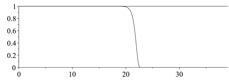
Figure 4: The rescaled function $s\to\phi(s\ln 10)$ approximating $1$ for $h=1$, $k_{1}=-2$, and $k_{2}=50$.

The practical feasibility of the approach depends on the representation of the tensors involved and the access to the Fourier transforms of the functions represented by them. An attractive choice are constructions based on Gauss-Hermite functions. Since the Fourier transforms of such functions are of the same type, the iterations do not lead out of this class. Approximations based on Gauss-Hermite functions are standard in quantum chemistry.

A central task not discussed here is the recompression of the data between the iteration steps in order to keep the amount of work and storage under control, a problem common to all tensor-oriented iterative methods. If one fixes the accuracy in the single coordinate directions, the process reduces to an iteration on the space of the functions defined on a given high-dimensional cubic grid, functions that are stored in a compressed tensor format. There exist highly efficient, linear algebra-based techniques for recompressing such data. A problem in the given context may be that the in this framework naturally looking discrete $\ell_{2}$-norm of the tensors does not match the underlying norms of the continuous problem. Another open question is the overall complexity of the process. A difficulty with our approach is that the given operators do not split into sums of operators that act separately on a single variable or a small group of variables, a fact that complicates the application of techniques such as of those in Bachmayr-Dahmen or Dahmen-DeVore-Grasedyck-Sueli . For more information on tensor-oriented solution methods for partial differential equations, see the monographs Hackbusch_1 and Khoromskij of Hackbusch and of Khoromskij and Bachmayr’s comprehensive survey article Bachmayr .

Appendix. Beta distributions and Jacobi polynomials

Setting $a=\beta-1$, $b=\alpha-1$, and introducing the constants

$$K(k,a,b)=\frac{2^{a+b+1}\,\Gamma(k+a+1)\Gamma(k+b+1)}{(2k+a+b+1)\Gamma(k+1)\Gamma(k+a+b+1)},$$

the density (28) can be rewritten in the form

$$f(t)=\,2\,\frac{b+1}{a+b+2}\,\frac{(1-x)^{a}(1+x)^{b}}{K(0,a,b)},\quad x={}-1+2\,\frac{b+1}{a+b+2}\;t.$$

The orthogonal polynomials $p_{k}$ from Lemma 10 assigned to this weight function $f$ can therefore be expressed in terms of the Jacobi polynomials

$$P_{k}^{(a,b)}(x)=P(k,a,b;x).$$

The Jacobi polynomials satisfy the orthogonality relation

$$\int_{-1}^{1}P(k,a,b;x)P(\ell,a,b;x)(1-x)^{a}(1+x)^{b}\,\mathrm{d}x=K(k,a,b)\delta_{k\ell}.$$

The polynomials $p_{k}$ therefore possess the representation

$$p_{k}(t)=\bigg{(}\frac{K(0,a,b)}{K(k,a,b)}\bigg{)}^{1/2}P\bigg{(}k,a,b;\,-1+2\,\frac{b+1}{a+b+2}\;t\,\bigg{)}.$$

At $x=-1$, the Jacobi polynomials take the value

$$P(k,a,b;\,-1)=(-1)^{k}\frac{\Gamma(k+b+1)}{\Gamma(k+1)\Gamma(b+1)},$$

see (Abramowitz-Stegun, , Table 22.4) or (DLMF, , Table 18.6.1). This leads to the closed representation

$$p_{k}(0)^{2}=\,\frac{(2k+a+b+1)\Gamma(a+1)\Gamma(k+b+1)\Gamma(k+a+b+1)}{\Gamma(a+b+2)\Gamma(b+1)\Gamma(k+1)\Gamma(k+a+1)}$$

of the values $p_{k}(0)^{2}$. Starting from $p_{0}(0)^{2}=1$, they can therefore be computed in a numerically very stable way by the recursion

$$p_{k+1}(0)^{2}=\,\frac{(k+b+1)(k+a+b+1)(2k+a+b+3)}{(k+1)(k+a+1)(2k+a+b+1)}\;p_{k}(0)^{2}.$$

An example

The following figure compares the distribution density originating from the matrix assigned to a small random graph, with no more than $m=32$ vertices and $n-m=96$ edges, with its approximation by the density of the corresponding normal distribution and that by the density of the corresponding rescaled beta distribution. The variance and the third-order central moment of the distribution are

$$V=\frac{941}{16640},\quad Z=\frac{97}{16640}.$$

The difference in the approximation quality is striking, but disappears for matrices assigned to larger graphs.

Supplement. Complete graphs and symmetry conservation

The goal in the background is to apply the developed techniques to approximate inverse iterations for the calculation of the ground state of the electronic Schrödinger equation; see Scholz-Yserentant for more details. Electronic wave functions are subject to the Pauli principle. Taking the spin into account, they are antisymmetric with respect to the exchange of the electrons, and if one considers the different spin components of the wave functions separately, they are antisymmetric with respect to the exchange of the electrons with the same spin. The following considerations show that such symmetry properties are preserved in the course of the calculations.

Since all electrons interact with each other, the matrix $T$ is in this case the matrix that is assigned to a complete graph, or better a triple copy of this matrix, one copy for each of the three spatial coordinates. We label the variables assigned to the vertices by the indices $i=1,\ldots,m$ and the variables assigned to the edges by the ordered index pairs $(i,j)$, $i<j$. The components of $Tx$ are in this notation

$$Tx|_{i}=x_{i},\quad Tx|_{i,j}=\frac{x_{i}-x_{j}}{\sqrt{2}}.$$

To every permutation $\pi$ of the vertices $i=1,\ldots,m$ associated with the positions of the electrons, we assign two matrices, the $(m\times m)$-permutation matrix $P$ given by

$$Px|_{i}=x_{\pi(i)},\quad i=1,\ldots,m,$$

and the much larger $(n\times n)$-matrix $Q$ given by

$$Qy|_{i}=y_{\pi(i)}$$

for the first $m$ components of $Qy$ associated with the vertices of the graph and by

$$Qy|_{ij}=\begin{cases}\;y_{\pi(i),\pi(j)},&\text{if $\pi(i)<\pi(j)$}\\ {}-y_{\pi(j),\pi(i)},&\text{otherwise}\end{cases}$$

for the remaining components associated with the edges. By construction then

$$TP=QT$$

holds, which is the key to the following considerations. As a permutation matrix, the matrix $P$ is orthogonal. The same holds for the matrix $Q$.

Lemma Up to sign changes, the matrix $Q$ is a permutation matrix.

Proof

Let the indices $i<j$ be given. If $\pi^{-1}(i)<\pi^{-1}(j)$, then

$$Qy|_{\pi^{-1}(i),\pi^{-1}(j)}=y_{ij}$$

holds, and if $\pi^{-1}(j)<\pi^{-1}(i)$ one has

$$Qy|_{\pi^{-1}(j),\pi^{-1}(i)}={}-y_{ij}.$$

All components of $y$ therefore also appear as components of $Qy$, either with positive or negative sign, just in a different order. ∎

Furthermore, we assign to the matrix $Q$ the value

$$\epsilon(Q)=\mathrm{sign}(\pi),$$

that is, the number $\epsilon(Q)=+1$, if $\pi$ consists of an even number of transpositions, and the number $\epsilon(Q)=-1$ otherwise.

Let $G$ be a subgroup of the symmetric group $S_{m}$, the group of the permutations of the indices $1,\ldots,m$. The matrices $P$ assigned to the elements of $G$ form a group which is isomorphic to $G$ under the matrix multiplication as composition. We say that a function $u:\mathbb{R}^{m}\to\mathbb{R}$ is antisymmetric under the permutations in $G$, or for short antisymmetric under $G$, if for all matrices $P=P(\pi)$ assigned to the $\pi\in G$

$$u(Px)=\mathrm{sign}(\pi)u(x)$$

holds. We say that a function $U:\mathbb{R}^{n}\to\mathbb{R}$ is antisymmetric under $G$ if for all these permutations $\pi$ and the assigned matrices $Q=Q(\pi)$

$$U(Qy)=\epsilon(Q)U(y)$$

holds. Both properties correspond to each other.

Lemma If the function $U:\mathbb{R}^{n}\to\mathbb{R}$ is antisymmetric under $G$, so are its traces.

Proof

This follows from the relation $TP=QT$ between the matrices. We have

$$U(TPx)=U(QTx)=\epsilon(Q)U(Tx).$$

Because of $\epsilon(Q)=\mathrm{sign}(\pi)$, the proposition follows. ∎

We say that a function $U:\mathbb{R}^{n}\to\mathbb{R}$ is symmetric under the permutations in $G$, or for short symmetric under $G$, if for all matrices $Q=Q(\pi)$, $\pi\in G$,

$$U(Qy)=U(y)$$

holds. Since the matrices $Q(\pi)$ assigned to the permutations in $\pi\in G$ are orthogonal, rotationally symmetric functions have this property.

In the following we show that for any right-hand side $F$ of the equation (9), which is antisymmetric under the permutations in $G$, its solution (10) is also antisymmetric under $G$ and that the same holds for the approximations of this solution.

Lemma If the function $F:\mathbb{R}^{n}\to\mathbb{R}$ possesses an integrable Fourier transform and is antisymmetric under $G$, then for any measurable and bounded kernel $K$, which is symmetric under $G$, the functions

$$U(y)=\bigg{(}\frac{1}{\sqrt{2\pi}}\bigg{)}^{n}\!\int K(\omega)\,\widehat{F}(\omega)\,\mathrm{e}^{\,\mathrm{i}\,\omega\cdot y}\,\mathrm{d}\omega$$

are antisymmetric under the permutations in $G$.

Proof

From the orthogonality of the matrices $Q=Q(\pi)$, $\pi\in G$, we obtain

$$U(Qy)=\bigg{(}\frac{1}{\sqrt{2\pi}}\bigg{)}^{n}\!\int K(Q\omega)\,\widehat{F}(Q\omega)\,\mathrm{e}^{\,\mathrm{i}\,\omega\cdot y}\,\mathrm{d}\omega$$

and in the same way the representation

$$\widehat{F}(Q\omega)=\bigg{(}\frac{1}{\sqrt{2\pi}}\bigg{)}^{n}\!\int F(Qy)\,\mathrm{e}^{\,-\mathrm{i}\,\omega\cdot y}\,\mathrm{d}y.$$

Because of $F(Qy)=\epsilon(Q)F(y)$, the Fourier transform of $F$ thus transforms like

$$\widehat{F}(Q\omega)=\epsilon(Q)\widehat{F}(\omega).$$

As by assumption $K(Q\omega)=K(\omega)$, the proposition follows. ∎

The norm $\|\omega\|$ of the vectors $\omega$ in $\mathbb{R}^{n}$ is symmetric under the permutations in $G$, but also the norm of the vectors $T^{t}\omega$ in $\mathbb{R}^{m}$. This follows from the interplay of the matrices $P$, $Q$, and $T$, which is expressed in the relation $TP=QT$ and leads to

$$\|T^{t}Q\omega\|=\|P^{t}T^{t}Q\omega\|=\|T^{t}Q^{t}Q\omega\|=\|T^{t}\omega\|.$$

This means that every kernel $K(\omega)$ which depends on the norms of $\omega$ and $T^{t}\omega$ only is symmetric under $G$. Provided that the right-hand side $F$ is antisymmetric under $G$, the same holds for the solution (10) of the equation (9) and for all its approximations calculated as described in the paper.

In summary, the solution of the equation (9) and all its approximations and their traces completely inherit the symmetry properties of the right-hand side. We conclude that our theory is fully compatible with the Pauli principle. What is still missing is a procedure for the recompression of the data between the single iteration steps that preserves the symmetry properties.

References

- (1) M. Abramowitz and I. A. Stegun, Handbook of mathematical functions, Dover Publications, New York, 10th printing in 1972.
- (2) M. Bachmayr, Low-rank tensor methods for partial differential equations, Acta Numerica 32 (2023), 1–121.
- (3) M. Bachmayr and W. Dahmen, Adaptive near-optimal rank tensor approximation for high-dimensional operator equations, Found. Comp. Math. 15 (2015), 839–898.
- (4) G. Beylkin and L. Monzón, Approximation by exponential sums revisited, Appl. Comput. Harmon. Anal. 28 (2010), 131–149.
- (5) D. Braess and W. Hackbusch, Approximation of by exponential sums in , IMA J. Numer. Anal. 25 (2005), 685–697.
- (6) , On the efficient computation of high-dimensional integrals and the approximation by exponential sums, Multiscale, Nonlinear and Adaptive Approximation (Berlin Heidelberg) (R. DeVore and A. Kunoth, eds.), Springer, 2009.
- (7) W. Dahmen, R. DeVore, L. Grasedyck, and E. Süli, Tensor-sparsity of solutions to high-dimensional elliptic partial differential equations, Found. Comp. Math. 16 (2016), 813–874.
- (8) S. Dasgupta and A. Gupta, An elementary proof of a theorem of Johnson and Lindenstrauss, Random Structures Algorithms 22 (2003), 60–65.
- (9) P. Frankl and H. Maehara, Some geometric applications of the beta distribution, Ann. Inst. Statist. Math. 42 (1990), 463–474.
- (10) W. Hackbusch, Computation of best exponential sums for by Remez’ algorithm, Computing and Visualization in Science 20 (2019), 1–11.
- (11) , Tensor spaces and numerical tensor calculus, Springer, Cham, 2019.
- (12) B. N. Khoromskij, Tensor numerical methods in scientific computing, Radon Series on Computational and Applied Mathematics, vol. 19, De Gruyter, Berlin München Boston, 2018.
- (13) F. W. J. Olver, D. W. Lozier, R. F. Boisvert, and C. W. Clark (eds.), NIST handbook of mathematical functions, Cambridge University Press, Cambridge, 2010.
- (14) S. Scholz and H. Yserentant, On the approximation of electronic wavefunctions by anisotropic Gauss and Gauss-Hermite functions, Numer. Math. 136 (2017), 841–874.
- (15) J. W. Siegel and J. Xu, Sharp bounds on the approximation rates, metric entropy, and n-widths of shallow neural networks, Found. Comput. Math. (2022).
- (16) B. Sturmfels, Algorithms in invariant theory, Springer, Wien, 2008.
- (17) B. L. van der Warden, Algebra I, Springer, Berlin Heidelberg New York, 1971.
- (18) R. Vershynin, High-dimensional probability, Cambridge University Press, Cambridge, 2018.
- (19) H. Yserentant, On the expansion of solutions of Laplace-like equations into traces of separable higher-dimensional functions, Numer. Math. 146 (2020), 219–238.
- (20) , A measure concentration effect for matrices of high, higher, and even higher dimension, SIAM J. Matrix Anal. Appl. 43 (2022), 464–478.