Scalable Learning of Item Response Theory Models

Abstract

Item Response Theory (IRT) models aim to assess latent abilities of $n$ examinees along with latent difficulty characteristics of $m$ test items from categorical data that indicates the quality of their corresponding answers. Classical psychometric assessments are based on a relatively small number of examinees and items, say a class of $200$ students solving an exam comprising $10$ problems. More recent global large scale assessments such as PISA, or internet studies, may lead to significantly increased numbers of participants. Additionally, in the context of Machine Learning where algorithms take the role of examinees and data analysis problems take the role of items, both $n$ and $m$ may become very large, challenging the efficiency and scalability of computations. To learn the latent variables in IRT models from large data, we leverage the similarity of these models to logistic regression, which can be approximated accurately using small weighted subsets called coresets. We develop coresets for their use in alternating IRT training algorithms, facilitating scalable learning from large data.

1 INTRODUCTION

Item Response Theory (IRT) is a paradigm often employed in psychometrics to estimate the ability of tested persons, called examinees, through tests comprising multiple questions, called items. The probability $p_{ij}$ that an item $i\in[m]:=\{1,\ldots,m\}$ will be solved by a person $j\in[n]$, depends on characteristic parameters of the item as well as on an ability parameter of the examinees.

The number of tested persons can be very large in contemporary global large scale assessments. For instance, the Programme for International Student Assessment (PISA) evaluates the education quality across $38$ OECD countries by measuring the literacy of $15$ year old students in reading, mathematics, and sciences. In this and other large scale (meta-)studies, nearly $n\approx 600\,000$ examinees are being tested regularly (Muncer et al.,, 2021; OECD,, 2019). The number of items in the case of PISA is, however, comparatively small, $m\approx 10-30$ in each category. Beyond educational applications, IRT can be applied to benchmark studies where the examinees are artificial intelligence agents or machine learning algorithms, and the items are various problems. Then, the number of both, items and examinees, can in principle become arbitrarily large (Martínez-Plumed et al.,, 2019). When the input data dimensions, $n$ and $m$, become large as motivated above, the computational effort to learn the parameters of IRT models grows. Sometimes it is not even possible to store the entire input or all latent variables simultaneously in main memory, which limits the applicability of IRT algorithms in large scale settings.

A basic algorithmic pattern for learning IRT models is an alternating optimization procedure akin to EM algorithms. This is a classical approach taught in standard undergraduate courses in psychology, and thus it is highly significant. Given fixed values for the ability parameters, we optimize the item specific difficulty characteristics. Then, the updated difficulty characteristics are fixed while the abilities are being optimized. These two steps constitute one phase that is iterated over and over again until some termination criterion is met, such as convergence or exhaustion of an iteration budget.

To make this algorithmic pattern scalable to large data, we note that especially learning the item parameters from a huge number of examinees takes considerable time and space to be processed. In automated settings with a large number of test items, the same situation appears in the second step of each phase. Here, we note that in simple so called 1PL and 2PL (one/two parameter logistic) IRT models, each step consists of solving a set of logistic regression problems, where only the labels differ for each examinee or item. For logistic regression, it is known how to handle large data in a time and memory efficient way using a succinct summary as a replacement for the data. Such a proxy is commonly known as a coreset that provably preserves the negative log-likelihood up to little errors (Munteanu and Schwiegelshohn,, 2018).

1.1 Our Contributions

We review and motivate IRT models for various tasks and from different perspectives, ranging from the educational and social sciences to machine learning, where scalable IRT algorithms become important. From this starting point

1. we leverage the similarity of 2PL IRT models to logistic regression and adapt previous coresets to facilitate scalable learning of 2PL models,

2. we develop new coresets for the more general and more challenging class of 3PL IRT models,

3. we empirically evaluate the computational benefits of coresets for IRT algorithms while preserving their statistical accuracy up to little distortions.

To our knowledge, our work provides the first sublinear approximation to the IRT subproblems considered in the alternating optimization steps with proven mathematical guarantees.

1.2 Related Work

Development of IRT

The history of IRT began with the formulation of the Rasch model (Rasch,, 1960). This was soon extended to modeling items with several parameters such as the 2PL and 3PL models (Birnbaum,, 1968). IRTs became popular in the United States through the book of Lord and Novick, (1968). Other extensions include models for items with several ordered categories (Masters,, 1982; Samejima,, 1969), and models with continuous data such as the 2PL model with beta distributions (Noel and Dauvier,, 2007). By now, IRT models are widely used for developing and scoring tests. For instance, large-scale assessments such as PISA (OECD,, 2009, 2019) and the Trends in International Mathematics and Science Study (TIMSS) (von Davier,, 2020) use IRT models for scoring responses, making them comparable between students who received different sets of items.

IRT in Machine Learning

To the best of our knowledge there are no rigorous theoretical guarantees on algorithms for learning the latent parameters of IRT models. Recently, IRT models have been used as a tool for analyzing machine learning classifiers (Martínez-Plumed et al.,, 2019). An extension building on beta distributions is the $\beta^{3}$-model by Chen et al., (2019) introduced and applied to assess the ability of machine learning classifiers. IRT was also introduced to ensemble learning (Chen and Ahn,, 2020). Recently, an IRT based analysis of regression algorithms and problems was suggested by Muñoz et al., (2021). Martínez-Plumed et al., (2022) proposed an empirical estimation for the difficulty of AI tasks using IRT models.

Coresets for Logistic Regression

Reddi et al., (2015) used gradient-based methods to construct coresets for logistic regression, though without a bound on their size. Later, Huggins et al., (2016) applied the framework of sensitivity sampling (Langberg and Schulman,, 2010) noting that there are instances that require linear size to be approximated. Munteanu et al., (2018) proved that compression below $\Omega(n)$ is not possible in general. They developed the first provably sublinear coresets for logistic regression on mild inputs $X$ of size $n$ and dimension $d$, introducing a data dependent parameter $\mu(X)$ to capture the complexity of compressing the data. This enabled a parameterized analysis giving a coreset, which for a given parameter $\varepsilon\in(0,1/2)$ provides a multiplicative approximation factor of $(1+\varepsilon)$ within size $\tilde{O}(\mu^{3}d^{3}/\varepsilon^{4})$, hiding polylogarithmic terms in $n$. This was recently improved to $\tilde{O}(\mu^{2}d/\varepsilon^{2})$ (Mai et al.,, 2021) by importance subsampling using $\ell_{1}$ Lewis weights as a replacement for the previous square root of $\ell_{2}$-leverage scores. More recently, it was extended to a single pass online algorithm along with a lower bound claiming linear dependence on $\mu$ (Woodruff and Yasuda, 2023a, ). Coresets for logistic regression were recently extended to $p$-generalized probit models (Munteanu et al.,, 2022) giving the first coresets in this line whose size are independent of $n$. There are further extensions to a certain class of near-convex functions (Tukan et al.,, 2020) and to monotonic functions (Tolochinsky et al.,, 2022).

2 PRELIMINARIES

IRT Models

There are various IRT models that are employed in the literature, mainly differing in their number of parameters used to describe the characteristics of examinees and items, respectively. Although an examinee can in principle be described using multiple parameters, a common choice is only one ability parameter, denoted $\theta_{j}$ for examinee $j\in[n]$. The number of parameters describing item characteristics varies more distinctively across IRT models, building or generalizing one over the other. The simplest of all is the Rasch model, named after its inventor (Rasch,, 1960), and is mathematically equivalent to the 1PL model. Here, one only takes into account how the ability $\theta_{j}$ differs from the difficulty $b_{i}$ of solving item $i$, expressed in units of the ability parameter $\theta_{j}$ (Baker and Kim,, 2004). The 2PL-model, introduced by Birnbaum, (1968), is a basic model that is most commonly used. It describes item $i$ introducing a discrimination or scale parameter $a_{i}$ in addition to its difficulty. The next step in this sequence of generalizations is adding to each item a default guessing parameter $c_{i}$, which leads us to the 3PL model. We note that there exist even more general 4PL models (Barton and Lord,, 1981). In this paper, however, we do not go into details about more general models than 3PL. Putting all parameters together in a probabilistic model, we arrive at the item characteristic curve (ICC) specifying the probability of passing test item $i$ depending on the ability parameter $\theta_{j}$:

$$p_{i}(\theta_{j})=c_{i}+\frac{1-c_{i}}{1+\exp(-a_{i}\theta_{j}+b_{i})},$$ (1)

The probability of an incorrect answer is consequently

$$1-p_{i}(\theta_{j})=\frac{1-c_{i}}{1+\exp(a_{i}\theta_{j}-b_{i})}.$$ (2)

We note that this defines a logistic sigmoid curve, see Figure 1, with a lower asymptote of $c_{i}\geq 0$.

We describe the interpretation of the parameters corresponding to an item $i$:

• The discrimination parameter $a_{i}$ specifies how flat or steep the curve ascends from $c_{i}$ to $1$. For example, a very steep ascend indicates that the item is nearly unsolvable unless the examinee has gained a special competence or knowledge. A knowledgeable examinee, however, is nearly guaranteed to pass the item. A flat curve indicates that the examinee needs to learn the necessary competences and gain some ’experience’ in solving the task.

• The difficulty parameter $b_{i}$ specifies the threshold where passing or failing the item have equal $0.5$ probability (when $c_{i}=0$). Examinees with a significantly smaller ability $\theta_{j}$ have a low probability of passing, while those with a much larger ability have a high probability of passing.

• Finally, the guessing parameter $c_{i}$ indicates the probability of passing, say a multiple choice item, by randomly answering the question without having any knowledge or ability for solving the task.

In the special case of $c_{i}=0$ for all $i$, Equation 1 simplifies to the 2PL model and further constraining $a_{i}=1$ for all $i$ yields the 1PL (Rasch) model.

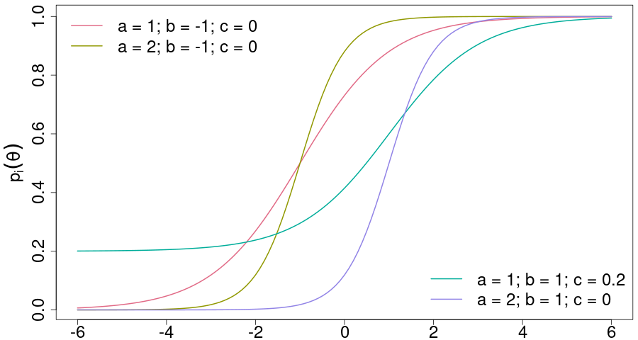
Figure 1: Item Characteristic Curve examples

The 2PL parameters are in principle unbounded, i.e., $a_{i},b_{i}\in\mathbb{R}$, though we may safely assume that $a_{i}>0$ to account for the reasonable fact that with growing ability it becomes more likely to solve an item, but the reverse situation never occurs. Another prior knowledge that we may assume for the additional guessing probability is that $c_{i}\in[0,0.5)$ since we do not want a randomly answered item to be solved with higher probability than a coin flip. In practical settings where we encounter multiple choice items we may often assume a lower bound such as $c_{i}>c_{\min}=1/\kappa$, where $\kappa$ is the number of offered choices.

The difficulty in learning IRT models as introduced above comes from the fact that all parameters are unobserved latent variables, meaning that they are neither given nor explicitly observed. The data only consists of binary observations $Y_{ij}\in\{-1,1\}$, indicating for item $i\in[m]$ and examinee $j\in[n]$ whether the item was answered correctly $Y_{ij}=1$ or not $Y_{ij}=-1$. For notational convenience, we let the data be arranged in a matrix $Y=(Y_{ij})_{i\in[m],j\in[n]}\in\{-1,1\}^{m\times n}$.

We stress that our coreset results are quite general in that they approximate the IRT model, and their use is not restricted to a specific algorithm. Nevertheless, we choose to build and evaluate our coresets on the following classical approach due to its high significance in standard undergraduate courses in psychology. Learning the latent parameters of IRT models involves a non-convex joint maximum likelihood optimization problem that encounters identifiability problems (San Martín et al.,, 2015). Due to the fact that the parameter space increases with the sample size, we need to condition on one set of parameters to optimize for the other. This yields an alternating two-step optimization approach that operates as follows (cf. Baker and Kim,, 2004):

General Algorithmic IRT Framework

1. Initialize all latent parameters.

2. While termination criterion is not met:

   1. Learn the ability parameters, given fixed item characteristics.

   2. Learn the item characteristics, given fixed ability parameters.

Starting from a proper initialization, the algorithm optimizes one set of parameters given the other until convergence (to a local optimum) is detected or a given iteration budget is exhausted. It is noteworthy that in the case of a 2PL IRT model, the two conditional optimization subproblems are not only convex but correspond exactly to standard logistic regression problems in two dimensions. The 3PL model, however, is more challenging, since it involves optimization over a combination of unbounded logistic loss functions as well as bounded non-convex sigmoid functions. We will elaborate on this in Section 3 below.

Coresets for the IRT Framework

Given massively large input data and a potential solution to an optimization problem, it is often already prohibitively expensive to evaluate or even to optimize the loss function with respect to the entire input. In such situations, it is preferable to have a much smaller subset of the data, such that solving the optimization problem on this small summary gives us an accurate approximate solution compared to the result obtained from analyzing the entire data.

This leads us to the concept of coresets that we want to compute in order to make the optimization steps 2(a) and 2(b) scalable to large data. Both can be treated similarly. For the sake of presentation, we thus focus on the optimization in step 2(b) since in most natural settings the number of examinees exceeds the number of items, i.e. $n\gg m$. The optimization step 2(b) can be decomposed into $m$ independent instances, indexed by $i\in[m]$, of the following form, each summing over the huge number of $n$ examinees: $f_{w}(X\eta_{i})=\sum_{j\in[n]}w_{j}g(x_{j}\eta_{i}),$ where $X$ is an $n\times d$ matrix comprising the currently fixed ability parameters as row vectors $x_{j}\in\mathbb{R}^{d}$, along with their corresponding labels $Y_{ij}$ from the data matrix, $\eta_{i}\in\mathbb{R}^{d}$ are vectors comprising the item characteristic parameters to be optimized in the current iteration, and $w\in\mathbb{R}^{n}$ is a vector of non-negative weights that is dropped from the notation whenever all weights equal $w_{j}=1$.

A significantly smaller subset $K\subseteq X,k:=|K|\ll|X|$ together with corresponding weights $u\in\mathbb{R}^{k}$ is a $(1+\varepsilon)$-coreset for $X$ if it satisfies that

$$\forall\eta\in\mathbb{R}^{d}\colon\lvert f_{w}(X\eta)-f_{u}(K\eta)\rvert\leq\varepsilon\cdot f_{w}(X\eta).$$ (3)

We refer to Definition A.1 in the appendix for details. Intuitively, a coreset evaluates for each possible solution to the same value as the original point set up to a factor of $(1\pm\varepsilon)$, and moreover it implies that the minimum obtained from optimizing over the coreset is within a $(1+O(\varepsilon))$ approximation to the original optimum (see Lemma A.26), while the memory and computational requirements are significantly reduced.

Unfortunately, $(1+\varepsilon)$-coresets of size $k\ll n$ cannot be obtained for the logistic regression problem in general. Thus, such coresets can neither exist for 2PL IRT models, nor for 3PL models. To facilitate an analysis beyond the worst case, a data dependent parameter $\mu$ was introduced by Munteanu et al., (2018), which can be used to bound the size of data summaries with the above accuracy guarantees and thus it enables a formal analysis and construction of small coresets for the logistic regression problem, as well as for other related problems. Their original definition will suffice for the 2PL model.

Here, we extend the definition slightly to impose that additionally to the $\ell_{1}$-norm ratio between the positive and the negative entries, also their fraction in terms of $\ell_{0}$-norm is bounded, i.e., the ratio of the number of positive and negative entries. This will be needed in our extension to the 3PL model. We let for $p\in\{0,1\}$

$$\mu_{p}(X)=\sup_{\eta\in\mathbb{R}^{d}\setminus\{0\}}\frac{\sum_{x_{i}\eta\geq 0}|x_{i}\eta|^{p}}{\sum_{x_{i}\eta<0}|x_{i}\eta|^{p}}=\sup_{\eta\in\mathbb{R}^{d}\setminus\{0\}}\frac{\|(X\eta)^{+}\|_{p}}{\|(X\eta)^{-}\|_{p}}$$

and say $X$ is $\mu_{p}$-complex if $\mu_{p}(X)\leq\mu_{p}$ for a bounded $1\leq\mu_{p}<\min\{m,n\}$. We say $X$ is $\mu$-complex if $\max\{\mu_{0},\mu_{1}\}\leq\mu<\min\{m,n\}$. It follows that

$$\|(X\eta)^{-}\|_{p}/\mu\leq\|(X\eta)^{+}\|_{p}\leq\mu\cdot\|(X\eta)^{-}\|_{p}.$$ (4)

For the left hand side inequality, note that for every $\eta$ the supremum also considers $-\eta$, for which the roles of positive and negative entries are reversed.

Constructing Coresets

Recall that the loss functions that we encounter when we train IRT models are defined as sums of individual point-wise losses. It is well-known from the related work on logistic regression that the multiplicative approximation guarantees provided by coresets cannot be obtained by uniform sampling. We elaborate on this with a focus on IRT in Appendix C for completeness of presentation.

A common method for obtaining coresets to approximate such functions by importance sampling is called the sensitivity framework that was introduced by Langberg and Schulman, (2010). They defined the sensitivity of an input point as their worst case individual contribution to the entire loss function. The sensitivity of a point $x_{j}$ for the function $f_{w}(X\eta)=\sum_{j\in[n]}w_{j}g(x_{j}\eta)$ is

$$\sigma_{j}=\sup_{\eta}\frac{w_{j}g(x_{j}\eta)}{f_{w}(X\eta)}.$$

This was subsequently combined with the theory of VC dimension to obtain a meta-theorem. It states that we can take a properly reweighted subsample using sampling probabilities that are proportional to the sensitivities. This yields a $(1+\varepsilon)$-coreset if its size is taken to be $k=O(\frac{S}{\varepsilon^{2}}(\Delta\log S+\log\frac{1}{\delta}))$. Here $S=\sum_{j\in[n]}\sigma_{j}$ denotes the total sensitivity, $\Delta$ denotes the VC dimension of a set system derived from the functions $g(x_{i}\eta)$, and $\delta$ is the failure probability (Feldman et al.,, 2020). One complication, however, is that computing the exact sensitivities is usually as hard as solving the problem under study. Fortunately, any upper bounds on the sensitivities suffice as a replacement. However their overestimation should be controlled carefully since the total sensitivity grows and is an important parameter that determines the coreset size. Further details on the sensitivity framework are in Section A.1. In the following we can assume that the problem of constructing coresets reduces to bounding the VC dimension and estimating the sensitivities for the functions under study.

3 CORESETS FOR IRT MODELS

3.1 2PL Models

For a suitable presentation of our technical results on coresets for IRT models, we use the following notation. For the item parameters, we define vectors $\alpha_{i}=(a_{i},b_{i})^{T},i\in[m]$ and similarly we define for the examinees $\beta_{j}=(\theta_{j},-1)^{T},j\in[n]$ and collect them in matrices $A=\begin{bmatrix}\alpha_{1}&\ldots&\alpha_{m}\end{bmatrix}\in\mathbb{R}^{2\times m}$ and $B=\begin{bmatrix}\beta_{1}&\ldots&\beta_{n}\end{bmatrix}\in\mathbb{R}^{2\times n}$. Now, given the item characteristics and the ability parameters, the probability of observing the data matrix $Y$ can be rewritten as

$$\mathbf{Pr}\left[Y|A,B\right]=\prod\nolimits_{i\in[m],j\in[n]}\frac{1}{1+\exp(-Y_{ij}\alpha_{i}^{T}\beta_{j})}.$$ (5)

To compute a joint maximum likelihood estimate of the item and ability parameters, a basic approach is to fix one set, say the item parameters $A$, and optimize over the ability parameters $B$, and then switch their roles. This process is repeated in an alternating manner (Baker and Kim,, 2004) as we introduced in the general algorithmic IRT framework, see Section 2. This leads us to minimizing the following negative log-likelihood function switching back and forth between the roles of data and variables:

$$f(A\mid B)=\sum\nolimits_{i\in[m],j\in[n]}\ln(1+\exp(-Y_{ij}\alpha_{i}^{T}\beta_{j}))=f(B\mid A).$$

In particular, for a given fixed $B\in\mathbb{R}^{2\times n}$, we can write $x_{j}=-Y_{ij}\beta_{j}^{T}$ for every $j\in[n]$, and then set $X_{(i)}=(x_{j})_{j\in[n]}\in\mathbb{R}^{n\times 2}$ for each $i\in[m]$ to optimize for

$$\min\nolimits_{\alpha_{i}\in\mathbb{R}^{2}}\sum\nolimits_{j\in[n]}\ln(1+\exp(x_{j}\alpha_{i})).$$ (6)

By symmetry, for a given fixed $A\in\mathbb{R}^{2\times m}$, we can write $x_{i}=-Y_{ij}\alpha_{i}^{T}$ for every $i\in[m]$, and set $X_{(j)}=(x_{i})_{i\in[m]}\in\mathbb{R}^{m\times 2}$ for each $j\in[n]$ to optimize for

$$\min\nolimits_{\beta_{j}\in\mathbb{R}^{2}}\sum\nolimits_{i\in[m]}\ln(1+\exp(x_{i}\beta_{j})).$$ (7)

Note that the objective functions given in Equations 6 and 7 are equivalent to plain logistic regression (cf. Munteanu et al.,, 2018), where coresets for logistic regression were constructed using the sensitivity framework. To obtain an upper bound on the sensitivity of the input, the authors related the single contributions of input points $x_{j}$ to the square root of the so called $\ell_{2}$-leverage scores: $l_{j}=\sup_{\eta\in\mathbb{R}^{d}\setminus\{0\}}{|x_{j}\eta|^{2}}/{\|X\eta\|_{2}^{2}}\;,$ a measure that can be derived from the row norms of an orthonormal basis for the space spanned by the data matrix, see Definition A.6 and Lemma A.7 for details.

However, in (Munteanu et al.,, 2018), the label vector $Y$ was a fixed vector in $\mathbb{R}^{n}$, while here, $Y$ is a matrix in $\mathbb{R}^{m\times n}$, i.e., we have to deal with a different label vector for each item, respectively for each ability parameter, that is fixed in one iteration, and thus the matrices $X_{(i)}$ differ across a large number of iterations. Fortunately, the leverage scores – only depending on the spanned subspace, not on its representation – are invariant to sign flips as we show in the next lemma.

Lemma 3.1.

Suppose we are given a matrix $X\in\mathbb{R}^{m\times n}$ (for any $m,n\in\mathbb{N}$) and an arbitrary diagonal matrix $D=(d_{ij})_{i\in[m],j\in[m]}$, with $d_{ij}\in\{-1,1\}$ if $i=j$, and $d_{ij}=0$ otherwise. Then the leverage scores of $X$ are the same as the leverage scores of $DX$.

This insight allows us to use the square root of the $\ell_{2}$-leverage scores of $A$, respectively $B$, as a fixed importance sampling distribution across all iterations where the same latent parameter matrix is involved as a fixed ’data set’ even though the signs may arbitrarily change in each iteration. Let us consider the optimization problem in Equation 6. Here, we are given the ability parameter matrix $B\in\mathbb{R}^{2\times n}$ and the label matrix $Y\in\mathbb{R}^{m\times n}$. We can directly use Theorem 15 of (Munteanu et al.,, 2018), for logistic regression in $d=2$ dimensions (with uniform weights) to get a small reweighted coreset for each optimization of an $\alpha_{i}\in\mathbb{R}^{2}$. To this end, we approximate the $\ell_{2}$-leverage scores $l_{j},j\in[n]$ of $B$ and sample a coreset proportional to $\sqrt{l_{j}}+1/n$, where $\sqrt{l_{j}}$ captures the importance of coordinates with a large linear contribution, and the augmented uniform $1/n$ is useful to capture small elements near zero that can dominate when their number is large, since their logistic loss is bounded below by a nonzero constant. As in (Munteanu et al.,, 2018), this yields a coreset whose size is dominated by an $O(\sqrt{n})$ factor which can be repeated recursively $O(\log\log n)$ times to decrease the dependence to $\operatorname{polylog}(n)$. Moreover, by Lemma 3.1 it suffices to sample one single coreset that is valid across all iterations $i\in[m]$ optimizing for $\alpha_{i}$ and whose size is only inflated by an additive $\log(m)$ term to control the overall failure probability using a union bound over the $m$ iterations. This yields the following theorem.

Theorem 3.2.

Let $X_{(i)}=(-Y_{ij}\beta_{j}^{T})_{j\in[n]}\in\mathbb{R}^{n\times 2}$ be $\mu_{1}$-complex, for each $i\in[m]$. Let $\varepsilon\in(0,1/2)$. There exists a weighted set $K\in\mathbb{R}^{k\times 2}$ of size $k\in\tilde{O}(\frac{\mu^{3}}{\varepsilon^{4}}(\log(n)^{4}+\log(m))$, that is a $(1+\varepsilon)$-coreset simultaneously for all $X_{(i)}$, $i\in[m]$ for the 2PL IRT problem. The coreset can be constructed with constant probability and in $\tilde{O}(n)$ time.

We note that despite the fact that there are more recent theoretical improvements such as (Mai et al.,, 2021; Munteanu et al.,, 2022), we build our results on the techniques of Munteanu et al., (2018). Even though an analogue of Lemma 3.1 can be proven for the scores of these references, the practical performance of the classic result is often better or only slightly worse than the competitors and at the same time it is significantly faster to compute (cf. Mai et al.,, 2021; Munteanu et al.,, 2022). Recent advances (Woodruff and Yasuda, 2023b, ) also improve theoretical bounds for the root leverage scores of Munteanu et al., (2018), which partially explain and corroborate their success in practical applications, though in a different setting from ours.

3.2 3PL Models

An often addressed concern about 3PL IRT models is the difficulty to properly estimate the guessing parameter $c_{i}$ (Baker and Kim,, 2004), since it is hard to distinguish between sufficiently high abilities, and a large guessing probability. Different to the 2PL model, the subproblem of optimizing the item characteristics, conditioned on fixed ability parameters is already non-convex. Thus, parameter estimation is significantly more challenging and can greatly benefit from an input size reduction. To this end, we now develop coresets for the 3PL model.

We would like to reduce the 3PL model to solving logistic regression problems, as we have done for the 2PL model, by first fixing the additional parameter $c_{i}$ in order to learn all other parameters $(a_{i},b_{i},\theta_{j})_{i\in[m],j\in[n]}$ as before, and at the end of one iteration of the main loop fix the other parameters in the model to optimize only for $c_{i},i\in[m]$. Unfortunately, if we would optimize the guessing parameter $c_{i}$ in this way, the optimizer would conclude that either $c_{i}=0$ or $c_{i}=1$ since the objectives are monotonic in $c_{i}$. Thus, we would never reach a realistic estimate for $c_{i}$.

Using the notation of Section 3.1, we cannot rewrite Equations 1 and 2 in a uniform way to express the probability of observing the label matrix $Y$ as in Equation 5. Although the guessing parameters $c_{i}$ are inseparable from the corresponding $a_{i},b_{i}$ parameters during optimization, we denote them in a separate vector $C=(c_{1},\ldots,c_{m})^{T}$. Then, we have that

$$\mathbf{Pr}\left[Y|A,B,C\right]=\prod\nolimits_{i\in[m],j\in[n]}^{[Y_{ij}=-1]}\left(\frac{1-c_{i}}{1+\exp(\alpha_{i}^{T}\beta_{j})}\right)\times\prod\nolimits_{i\in[m],j\in[n]}^{[Y_{ij}=1]}\left(c_{i}+\frac{1-c_{i}}{1+\exp(-\alpha_{i}^{T}\beta_{j})}\right),$$ (8)

where the products iterate only over all indexes in the subscript, that satisfy the condition in the superscript. Similar notations are used for the sums below. Let $g_{i}(z)=-\ln(\frac{1-c_{i}}{1+\exp(z)})=\ln(1+\exp(z))-\ln(1-c_{i})$ and $h_{i}(z)=-\ln(c_{i}+\frac{1-c_{i}}{1+\exp(-z)})$. The general algorithmic IRT framework with an alternating optimization, see Section 2, that we already dealt with for the 2PL models, can be applied to the 3PL models as well for the following objective function

$$f(A,C\mid B)=f(B\mid A,C)=\sum_{i\in[m],j\in[n]}^{[Y_{ij}=-1]}g_{i}(-Y_{ij}\alpha_{i}^{T}\beta_{j})+\sum_{i\in[m],j\in[n]}^{[Y_{ij}=1]}h_{i}(-Y_{ij}\alpha_{i}^{T}\beta_{j}).$$

Let us assume that $A$ and $C$ are fixed, the other case will be addressed later. As in the case of 2PL we can write $x_{i}=-Y_{ij}\alpha_{i}^{T}$, for each $i\in[m]$, and $X_{(j)}=\left(x_{i}\right)_{i\in[m]}\in\mathbb{R}^{m\times 2}$. Then, we aim at minimizing for each $j\in[n]$ over $\beta_{j}\in\mathbb{R}^{2}$, the objective

$$f(\beta_{j}\mid A,C)=\sum\nolimits_{i\in[m]}^{\left[Y_{ij}=-1\right]}g_{i}(x_{i}\beta_{j})+\sum\nolimits_{i\in[m]}^{\left[Y_{ij}=1\right]}h_{i}(x_{i}\beta_{j}).$$ (9)

For all $z$ it holds that $g_{i}(z)>0$ and $h_{i}(z)>0$. The functions $g_{i}(z)$ and $h_{i}(z)$ have different shapes and cannot be represented as a single function. In particular, all functions $g_{i}(z)$ are similar to the logistic regression loss up to an additive shift of $-\ln(1-c_{i})$, with $0\leq-\ln(1-c_{i})<\ln 2$, since $c_{i}\in[0,0.5)$. The others, $h_{i}(z)$, are sigmoid functions satisfying $0<h_{i}(z)<\ln\left(1/c_{i}\right)$, for all values of $z$.

In the 3PL case, assuming that each matrix $X_{(j)}$ is $\mu_{1}$-complex does not give sufficient bounds for the distribution of input points to the two different types of functions. Therefore we split $X_{(j)}$ into submatrices $X_{(j)}^{\prime}$, containing the rows indexed by $i$ with labels $Y_{ij}=-1$, and $X_{(j)}^{\prime\prime}$ containing the rows with $Y_{ij}=1$. Now, we assume that $X_{(j)}^{\prime}$ and $X_{(j)}^{\prime\prime}$ are both $\mu$-complex, and $\sup_{\eta\in\mathbb{R}\setminus\{0\}}{\|X^{\prime}_{(j)}\eta\|_{1}}/{\|X^{\prime\prime}_{(j)}\eta\|_{1}}\leq 2\mu_{1}.$

The detailed technical analysis is deferred to the appendix due to page limitations. Here, we only give a high level description. We first upper bound the sensitivities for both types of functions separately and show that the total sensitivity over all functions remains sublinear. To this end consider the set of (shifted) logistic functions $g_{i}$. Those can be handled using the $\mu_{1}$-complexity of $X^{\prime}_{(j)}$ as in (Munteanu et al.,, 2018) up to technical modifications and adjusting constants.

For the second set of sigmoid functions $h_{i}$ we use the $\mu_{0}$-complexity property of both sets to bound the total number of elements in $X^{\prime}_{(j)}$ and $X^{\prime\prime}_{(j)}$ from below. This is needed to obtain uniform upper bounds for the sensitivities across all labelings, which together with Lemma 3.1 assures that one coreset suffices across all iterations $j\in[n]$. We further leverage the $\mu_{0}$-complexity of $X^{\prime\prime}_{(j)}$ to conclude that the fraction of positive elements in $X^{\prime\prime}_{(j)}\beta_{j}$ is sufficiently large.

The final open issue is to bound the VC dimension. Again, we handle both sets of functions separately. Since both types of functions are strictly monotonic and invertible tranformations of a dot product, they can be related to a set of affine separators that have bounded VC dimension of $d+1=3$ (Kearns and Vazirani,, 1994). By a classic result of Blumer et al., (1989) the VC dimension of the union of both sets of functions can be bounded by $O(d+1)$. Leveraging the disjointness of our sets, we can give a simpler proof that leads to a bound of $2(d+1)=6$. Another union over $O(\log m)$ weight classes concludes the VC dimension bound of $O(\log m)$. This yields our second main result:

Theorem 3.3.

Let each $X_{(j)}=(-Y_{ij}\alpha_{i}^{T})_{i\in[m]}\in\mathbb{R}^{m\times 2}$. Let $X^{\prime}_{(j)}$ contain the rows $i$ of $X_{(j)}$ where $Y_{ij}=-1$ and let $X^{\prime\prime}_{(j)}$ comprise the rows with $Y_{ij}=1$. Let $X^{\prime}_{(j)}$ and $X^{\prime\prime}_{(j)}$ be $\mu$-complex, and $\sup_{\eta\in\mathbb{R}\setminus\{0\}}\frac{\|X^{\prime}_{(j)}\eta\|_{1}}{\|X^{\prime\prime}_{(j)}\eta\|_{1}}\leq 2\mu_{1}$ for each $j\in[n]$. Let $\varepsilon\in(0,1/2)$. There exists a weighted set $K\in\mathbb{R}^{k\times 2}$ of size $k\in O(\frac{\mu^{2}\sqrt{m}}{\varepsilon^{2}}(\log(m)^{2}+\log(n)))$, that is a $(1+\varepsilon)$-coreset for all $X_{(j)}$, $j\in[n]$ simultaneously for the 3PL IRT problem. The coreset can be constructed with constant probability and in $O(m)$ time.

The remaining case $f(A,C\mid B)$ requires another $\frac{\mu^{2}}{\varepsilon}$ factor. The analysis is deferred to Appendix A due to page limitations. The discussion starts above Lemma A.22. In addition, we provide a parameter estimation guarantee for $\tau$-PL, with $\tau\in\{2,3\}$:

Theorem 3.4 (Informal version of Theorem A.25 in Section A.6).

Assume the conditions of Theorem 3.2 resp. Theorem 3.3. Then the optimal solutions for the $\tau$-PL problem, for $\tau\in\{2,3\}$, on the full input ($\eta_{\text{opt}}$) and on the coreset ($\eta_{\text{core}}$) satisfy

$$\|\eta_{\text{opt}}-\eta_{\text{core}}\|_{1}\leq O(\mu^{\tau-1})\cdot f(X\eta_{\text{opt}}).$$

4 EXPERIMENTS

All experiments were run on a HPC workstation with AMD Ryzen Threadripper PRO 5975WX, 32 cores at 3.6GHz, 512GB DDR4-3200. Our Python code implements the IRT framework introduced in Section 2 where Steps 2(a) and 2(b) solve Eq. (6) and (7), resp. their 3PL variants. The coreset is only computed in step 2(b) for reducing the number of examinees, i.e., the dominating dimension $n$, since the number of items $m$ is relatively small in our data; the coreset construction would dominate over analyzing the complete data.

Experimental Setup

We focus on 2PL models, which can be estimated more stably, as discussed before. We generate synthetic 2PL/3PL data by drawing item and ability parameters for each $j\in[n]$, $i\in[m]$ from the following distributions: $a_{i}\sim N(2.75,0.3)$ truncated at $0$, $b_{i}\sim N(0,1)$ and $\theta_{j}\sim N(0,1)$. For 2PL, we fix $c_{i}=0$, and for 3PL, we truncate $c_{i}\sim N(0.1,0.1)$ within $[0,0.5)$. The response probabilities $p_{ij}:=p_{i}(\theta_{j})$ are computed as in Equation 1. Each label is drawn from a Bernoulli distribution with the corresponding response probability, i.e., $Y_{ij}\sim\operatorname{Bernoulli}(p_{ij})$. We also use real world data (see their dimensions in Table 1): SHARE (Börsch-Supan,, 2022), measuring health indication of elderly Europeans, and NEPS (Blossfeld and Roßbach,, 2019; NEPS-Network,, 2021), measuring high school abilities of ninth grade students.

In our estimation algorithm, the ability parameters $\theta_{j}$ and the item difficulties $b_{i}$ are bounded by $b_{i},\theta_{j}\in[-6,6]$, and the item discrimination parameters are bounded by $a_{i}\in(0,5]$. Without imposing identification restrictions, the scale of estimated IRT parameters $a$, $b$, and $\theta$ is arbitrary. Therefore, we rescale them to obtain standardized parameters. To this end, we subtract the mean of $\theta$ from each $b_{i}$, multiply $a_{i}$ by the standard deviation of $\theta$ and finally standardize $\theta$ to zero mean and unit variance.

We vary the number of examinees $n$, the number of items $m$, and the size of the coreset $k$. For every combination we run 50 iterations of the main loop. Each experiment is repeated 20 times. We report results for a few selected configurations in Tables 1, 2 and 3. The majority of the results is in Appendix B.

Since $\mu$ is a crucial complexity parameter, we estimate its value for all different data sets in Appendix F. The majority and mean values for $\mu$ are small constants ranging between 2 and 20. Only in rare cases $\mu$ takes large maximum values for some label vectors. We checked the corresponding labels, and found that the large values occur only in degenerate cases, in which the maximum likelihood estimator of the model is undefined, for example, when an item is solved by all or none of the students.

Computational Savings

The parameter estimation using coresets is significantly faster than using the full input set. The coresets use only a small fraction of the memory used by the full data, while approximating the objective function very closely.

For the 2PL models on the synthetic data sets, the running time gains were at least $32\,\%$ and up to $66\,\%$ (see Tables 1 and 2). At the same time, the amount of memory used never exceeds $1\,\%$ of the original size. The largest instances we found across the literature are $n\approx 500\,000$ (OECD,, 2019) and $m\approx 5\;000$ (Muñoz et al.,, 2021). We added a synthetic example of this size whose total running time (for a single repetition) was reduced from $6.5$ to $3.8$ days. Besides running time, the memory spent for this large experiment is larger than 5 GB, impossible to be handled by standard psychometric tools.

For the real-world data sets, SHARE (Börsch-Supan,, 2022) and NEPS (NEPS-Network,, 2021), we show that a relative error of $\hat{\varepsilon}=0.05$ can be achieved using less than $6\,\%$ of the memory used when working on the full data. For the (relatively small) NEPS data set, the running time gain was about $30\,\%$, except when the coreset sizes exceed half of the input size. We note that for the SHARE data set, the running time gains are small, and can even be (slightly) negative. This is due to its very small original dimensions (especially $m=10$), for which the time for the coreset construction can dominate the overall running time.

For 3PL models, solving the original problem is more difficult and thus takes longer. Indeed, the subproblems estimating the sets of parameters in each phase are non-convex and cause the computational issues discussed in Section 3.2. As a consequence, reducing the input size increases the running time gain up to $86\,\%$ (see Tables 1 and 6). The memory used by the coresets is between $5\,\%$ and $20\,\%$ of the original data.

The data dimensions considered across our experiments are huge compared to data that is usually collected for IRT studies. On the other hand, even the largest data dimensions, are chosen small enough to be able to estimate the models on the full data set. However, our theoretical results prove that the subsample grows sublinearly with arbitrarily increasing data, showing the potential for larger future data.

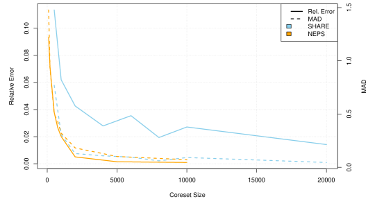
Figure 2: 2PL Experiments on real world SHARE and NEPS data: Coreset sizes vs. relative error and mean absolute deviation (MAD), cf. Tables 4 and 9.

Table 1: Mean running times (in minutes) taken across $20$ repetitions (of $50$ iterations of the main loop) per data set 2-/3-PL, (Sy)nthetic, SH(ARE), NE(PS), for different configurations of their data dimensions: number of items $m$, number of examinees $n$, and coreset size $k$. The (relative) gain is defined as $(1-\mathrm{mean}_{\textsf{core}}/\mathrm{mean}_{\textsf{full}})\cdot 100\,\%$. For the quality of the solutions, let $f_{\sf full}$ and $f_{{\sf core}(j)}$ be the optimal objective values on the input and on the coreset for the $j$-th repetition, resp. Let $f_{\sf core}=\min_{j}f_{{\sf core}(j)}$. Relative error: r.err. $\hat{\varepsilon}=|f_{\sf core}-f_{\sf full}|/f_{\sf full}$ (cf. Lemma A.26). Mean Absolute Deviation: $\textbf{mad}(\alpha)=\frac{1}{n}\sum(|a_{\textsf{full}}-a_{\textsf{core}}|+|b_{\textsf{full}}-b_{\textsf{core}}|+|c_{\textsf{full}}-c_{\textsf{core}}|)$; $\textbf{mad}(\theta)=\frac{1}{m}\sum|\theta_{\textsf{full}}-\theta_{\textsf{core}}|$, evaluated on the parameters attaining the optimal $f_{\textsf{full}}$ and $f_{\sf core}$.

data	$\mathbf{n},\mathbf{m},\mathbf{k}$	$\textbf{mean}_{\textsf{full}}(\text{min})$	$\textbf{mean}_{\textsf{core}}(\text{min})$	gain	r.err. $\hat{\varepsilon}$	$\text{mad}(\alpha)$	$\text{mad}(\theta)$
2PL-Sy	$50\,000,500,500$	$136.981$	$45.547$	$66.749\,\%$	$0.04803$	$0.525$	$0.008$
2PL-Sy	$100\,000,200,1\,000$	$122.252$	$61.459$	$49.727\,\%$	$0.03404$	$0.379$	$0.008$
2PL-Sy	$500\,000,500,5\,000$	$1\,278.845$	$591.878$	$53.718\,\%$	$0.01445$	$0.171$	$0.001$
2PL-Sy	$500\,000,5\,000,5\,000$	$9\,363.750$	$5\,536.684$	$40.871\,\%$	$0.00076$	$0.120$	$0.013$
2PL-SH	$138\,997,10,8\,000$	$28.853$	$27.637$	$4.216\,\%$	$0.01935$	$0.061$	$0.007$
2PL-NE	$11\,532,88,1\,000$	$5.968$	$4.009$	$32.829\,\%$	$0.02007$	$0.320$	$0.045$
3PL-Sy	$50\,000,100,10\,000$	$211.468$	$93.780$	$55.653\,\%$	$0.00212$	$0.384$	$0.010$
3PL-Sy	$50\,000,200,10\,000$	$369.816$	$145.674$	$60.609\,\%$	$0.02186$	$0.488$	$0.001$
3PL-Sy	$200\,000,100,10\,000$	$893.183$	$196.802$	$77.966\,\%$	$0.01789$	$0.524$	$0.003$

Figure 3: Parameter estimates for the coresets compared to the full data sets. The first row shows the bias for the item parameters $a,b$ (and $c$ for 3PL). The vertical axis is scaled to display $2\,{\mathrm{std.}}$ ($4\,{\mathrm{std.}}$ for 3PL) of the parameter estimate obtained from the full data set. The second row shows a kernel density estimate for the ability parameters $\theta$, standardized to zero mean and unit variance, with a LOESS regression line in dark green.

2PL Syn: $\mathbf{n=500\,000,m=500,k=5\,000}$	2PL NEPS: $\mathbf{n=11\,532,m=88,k=1\,000}$	3PL Syn: $\mathbf{n=50\,000,m=100,k=10\,000}$

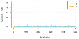
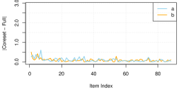
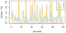
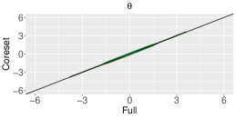
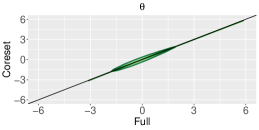
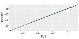
Parameter Estimation Accuracy

Overall, we find that incorporating coresets leads to comparable estimates as on the full data set. The differences are larger for 3PL. The bounded $\ell_{1}$ norm deviation (see Theorem 3.4/A.25) explains that either small errors are evenly distributed over many parameters, or large deviations affect only a few spikes. The accuracy clearly improves with increasing coreset size, cf. Tables 1 and 2, and Appendix B, especially Tables 3 and 9. Our coresets compare favorably against the results obtained from uniform sampling, and clustering coresets as baselines, cf. Appendices C and D. They also compare similarly to $\ell_{1}$ Lewis weights and $\ell_{1}$ leverage scores, see Appendix E.

For the 2PL models, the bias for the parameters estimated on the coresets in comparison to the full data sets are small and negligible in comparison to the scale of the parameter, see Figure 3. For the 3PL models, the bias is larger. This is because the item parameters of the 3PL model are not identifiable (San Martín et al.,, 2015) in the estimation approach, where even the sub-problems are non-convex. In this case, the coresets and the full data set (or, similarly, different starting values) may lead to different parameter estimates although they have a similar likelihood. Indeed, the close likelihood approximation provided by coresets not only mimics good model fit. Even when the model fits badly, it ensures that a proper diagnosis for detecting misspecification can be performed on coresets. For the ability parameters $\theta$ in 2PL models, the estimates are almost identical between the coresets and the full data. For 3PL, the estimates are bi-modal due to multiple local optima (Figure 3, bottom right).

5 CONCLUSIONS

We develop coresets to facilitate scalable and efficient learning of large scale Item Response Theory models. Coresets enable significantly larger IRT studies and will hopefully motivate larger surveys. Our implementation and experiments illustrate that standard algorithms for IRT can greatly benefit from using coresets in the estimation process. We observe large computational savings as well as accurate parameter recovery on a small but carefully selected fraction of the large data. We note that in our experiments, estimates were recovered with negligible errors when using coresets. Future research could incorporate coresets into state of the art IRT solvers that are more complicated than the standard approach but achieve much better estimation accuracy already on the original data. Further, it would be interesting to develop coresets for more general IRT models, including (ordered) categorical (Masters,, 1982), continuous (Chen et al.,, 2019), multidimensional (DeMars,, 2016), and multilevel (Adams et al.,, 1997) IRT models. Other interesting avenues are to extend to probit IRT models (Munteanu et al.,, 2022) or to incorporate sketching for logistic regression (Munteanu et al.,, 2021, 2023; Munteanu,, 2023) such as to avoid storing the full latent parameter matrices.

Appendix A OMITTED PROOFS

A.1 Technical Details on the Sensitivity Framework

Definition A.1 (Coreset, cf. Feldman et al.,, 2020).

Let $X\in\mathbb{R}^{n\times d}$ be a set of points $\{x_{1},\ldots,x_{n}\}$, weighted by $w\in\mathbb{R}_{>0}^{n}$. For any $\eta\in\mathbb{R}^{d}$, let the cost of $\eta$ w.r.t. the point $x_{i}$ be described by a function $w_{i}\cdot f\left(x_{i}\eta\right)$ mapping from $\mathbb{R}$ to $(0,\infty)$. Thus, the cost of $\eta$ w.r.t. the (weighted) set $X$ is $f_{w}\left(X\eta\right)=\sum_{i}w_{i}\cdot f\left(w_{i}\eta\right)$. Then a set $K\in\mathbb{R}^{k\times d}$, (re)weighted by $u\in\mathbb{R}_{>0}^{k}$ is a $(1+\varepsilon)$-coreset of $X$ for the function $f_{w}$ if $k\ll n$ and

$$\forall\eta\in\mathbb{R}^{d}\colon\left\lvert f_{w}\left(X\eta\right)-f_{u}\left(K\eta\right)\right\rvert\leq\varepsilon\cdot f_{w}\left(X\eta\right).$$

In our analysis we use sampling based on so-called sensitivity scores, the range space induced by the set of functions, and the VC-dimension. We define these notions next.

Definition A.2 (Sensitivity, (Langberg and Schulman,, 2010)).

Consider a family of functions $\mathcal{F}=\{g_{1},\ldots,g_{n}\}$ mapping from $\mathbb{R}^{d}$ to $[0,\infty)$ and weighted by $w\in\mathbb{R}_{>0}^{n}$. The sensitivity of $g_{\ell}$ for the function $f_{w}(\eta)=\sum_{\ell\in[n]}w_{\ell}g_{\ell}(\eta)$, where $\eta\in\mathbb{R}^{d}$, is

$$\sigma_{\ell}=\sup\frac{w_{\ell}g_{\ell}(\eta)}{f_{w}(\eta)},$$ (10)

The total sensitivity is $\mathfrak{S}=\sum_{\ell\in[n]}\sigma_{\ell}$.

Definition A.3 (Range space; VC dimension).

A range space is a pair $\mathfrak{R}=\left(\mathcal{F},\verb|ranges|\right)$, where $\mathcal{F}$ is a set and $\verb|ranges|$ is a family of subsets of $\mathcal{F}$. The VC dimension $\Delta(\mathfrak{R})$ of $\mathfrak{R}$ is the size $|G|$ of the largest subset $G\subseteq\mathcal{F}$ such that $G$ is shattered by $\verb|ranges|$, i.e., $|\{G\cap R:R\in\verb|ranges|\}|=2^{|G|}$.

Definition A.4 (Induced range space).

Let $\mathcal{F}$ be a finite set of functions mapping from $\mathbb{R}^{d}$ to $\mathbb{R}_{\geq 0}$. For every $x\in\mathbb{R}^{d}$ and $r\in\mathbb{R}_{\geq 0}$, let $\verb|range|_{\mathcal{F}}(x,r)=\{f\in\mathcal{F}:f(x)\geq r\}$, and $\verb|ranges|(\mathcal{F})=\{\verb|range|_{\mathcal{F}}(x,r):x\in\mathbb{R}^{d},r\in\mathbb{R}_{\geq 0}\}$. Let $\mathfrak{R}_{\mathcal{F}}=\left(\mathcal{F},\verb|ranges|(\mathcal{F})\right)$ be the range space induced by $\mathcal{F}$.

To construct coresets for the IRT models, we use a framework that combines sensitivity scores with the theory of VC dimension, originally proposed by Braverman et al., (2016, 2021). We employ a more recent and slightly modified version, stated in the following theorem.

Theorem A.5 (Feldman et al.,, 2020, Theorem 31).

Consider a family of functions $\mathcal{F}=\{f_{1},\ldots,f_{n}\}$ mapping from $\mathbb{R}^{d}$ to $[0,\infty]$ and a vector of weights $w\in\mathbb{R}_{>0}^{n}$. Let $\varepsilon,\delta\in(0,1/2)$. Let $s_{i}\geq\sigma_{i}$. Let $S=\sum_{i=1}^{n}s_{i}\geq\mathfrak{S}$. Given $s_{i}$ one can compute in time ${O\left(|\mathcal{F}|\right)}$ a set $\mathcal{R}\subset\mathcal{F}$ of

$${O\left(\frac{S}{\varepsilon^{2}}\left(\Delta\log S+\log\frac{1}{\delta}\right)\right)}$$

weighted functions such that with probability $1-\delta$ we have for all $\eta\in\mathbb{R}^{d}$ simultaneously

$$\left\lvert\sum_{f\in\mathcal{F}}w_{i}f_{i}(\eta)-\sum_{f\in\mathcal{R}}u_{i}f_{i}(\eta)\right\rvert\leq\varepsilon\sum_{f\in\mathcal{F}}w_{i}f_{i}(\eta),$$

where each element of $\mathcal{R}$ is sampled i.i.d. with probability $p_{j}=\frac{s_{j}}{S}$ from $\mathcal{F}$, $u_{i}=\frac{Sw_{j}}{|\mathcal{R}|s_{j}}$ denotes the weight of a function $f_{i}\in\mathcal{R}$ that corresponds to $f_{j}\in\mathcal{F}$, and where $\Delta$ is an upper bound on the VC dimension of the range space $\mathfrak{R}_{\mathcal{F}^{*}}$ induced by $\mathcal{F}^{*}$ that can be defined by defining $\mathcal{F}^{*}$ to be the set of functions $f_{j}\in\mathcal{F}$ where each function is scaled by $\frac{Sw_{j}}{|\mathcal{R}|s_{j}}$.

Note that Theorem A.5 does not put additional requirements on the set of the functions $\mathcal{F}$ besides an upper bound on the sensitivities, and a bounded VC-dimension of the range space induced by those functions.

A.2 Omitted Proofs for the 2PL Model

Definition A.6 (Leverage scores, cf. Drineas et al.,, 2012).

Given an arbitrary matrix $X\in\mathbb{R}^{m\times d}$, with $m>d$, let $U$ denote the $m\times d$ matrix consisting of the $d$ left singular vectors of $X$, and let $u_{i}$ denote the $i$-th row of the matrix $U$ as a row vector, for all $i\in[m]$. The $i$-th leverage score corresponding to row $x_{i}$ of $X$ is given by

$$l_{i}=\|u_{i}\|_{2}^{2}.$$

Lemma A.7.

Let $X=U\Sigma V^{T}$ be the singular value decomposition of $X$. The three definitions are equivalent:

1. The $i$-th leverage score (corresponding to row $x_{i}$) is given by

   $$l_{i}=\|u_{i}\|_{2}^{2}.$$

2. The $i$-th leverage score is given by

   $$l_{i}=\sup_{\eta\in\mathbb{R}^{d}\setminus\{0\}}\frac{|x_{i}\eta|^{2}}{\|X\eta\|_{2}^{2}}.$$

3. The $i$-th leverage score is given by

   $$l_{i}=e_{i}^{T}X\left(X^{T}X\right)^{-1}X^{T}e_{i}$$

Proof.

Statement 1 is equivalent to Definition A.6 since the SVD yields $U$, which is exactly the matrix of the left singular vectors of $X$.

Statement 2 is equivalent to Statement 1 since by a change of basis

$$l_{i} =\sup_{\eta\in\mathbb{R}^{d}\setminus\{0\}}\frac{|x_{i}\eta|^{2}}{\|X\eta\|_{2}^{2}}=\sup_{\eta\in\mathbb{R}^{d}\setminus\{0\}}\frac{|u_{i}\eta|^{2}}{\|U\eta\|_{2}^{2}}\stackrel{{\scriptstyle CSI}}{{\leq}}\frac{\|u_{i}\|_{2}^{2}\|\eta\|_{2}^{2}}{\|U\eta\|_{2}^{2}}=\frac{\|u_{i}\|_{2}^{2}\|\eta\|_{2}^{2}}{\|\eta\|_{2}^{2}}=\|u_{i}\|_{2}^{2}.$$

The conclusion follows from the Cauchy-Schwarz inequality (CSI) and the fact that $U$ is an orthonormal matrix. The inequality is tight due to the supremum over all $\eta\in\mathbb{R}^{d}$ and the existence of $\eta^{*}=u_{i}^{T}\in\mathbb{R}^{d}$ that realizes equality in CSI.

Let $e_{i}$, for $i\in[m]$, be the standard basis vectors in $\mathbb{R}^{m}$ containing $1$ as $i$-th coordinate, and $0$ everywhere else.

$$l_{i} =e_{i}^{T}X\left(X^{T}X\right)^{-1}X^{T}e_{i}$$

$$=e_{i}^{T}U\Sigma V^{T}\left(V\Sigma U^{T}U\Sigma V^{T}\right)^{-1}V\Sigma U^{T}e_{i}=e_{i}^{T}U\Sigma V^{T}\left(V\Sigma^{2}V^{T}\right)^{-1}V\Sigma U^{T}e_{i}$$

$$=e_{i}^{T}U\Sigma V^{T}V\Sigma^{-2}V^{T}V\Sigma U^{T}e_{i}=e_{i}^{T}U\Sigma\Sigma^{-2}\Sigma U^{T}e_{i}$$

$$=e_{i}^{T}UU^{T}e_{i}=u_{i}u_{i}^{T}=\|u_{i}\|_{2}^{2}$$

since $U$ and $V$ are orthonormal matrices, and $\Sigma$ is a square diagonal matrix. ∎

Lemma A.8 (Restatement of Lemma 3.1).

Suppose we are given a matrix $X\in\mathbb{R}^{m\times n}$ (for any $m,n\in\mathbb{N}$) and an arbitrary diagonal matrix $D=(d_{ij})_{i\in[m],j\in[m]}$, with $d_{ij}\in\{-1,1\}$ if $i=j$, and $d_{ij}=0$ otherwise. Then the leverage scores of $X$ are the same as the leverage scores of $DX$.

Proof.

Let $D=\mathrm{diag}(\{-1,1\}^{m})$ be chosen as in the statement. Then it holds that $D^{2}=D^{T}D=I_{m}$. Further it holds that $e_{i}^{T}D=d_{ii}e_{i}^{T}$, where $e_{i}$ denotes the $i$th standard basis vector, i.e., the vector containing a $1$ as its $i$-th coordinate, and zeros everywhere else. The $i$-th leverage score of $X$ can be expressed as $\ell_{i}=e_{i}^{T}X\left(X^{T}X\right)^{-1}X^{T}e_{i}$ by Lemma A.7 (cf. Drineas et al.,, 2012). Similarly, for the $i$-th leverage score $\tilde{\ell}_{i}$ of $DX$ we have that

$$\tilde{\ell}_{i} =e_{i}^{T}(DX)\left(X^{T}D^{T}DX\right)^{-1}(X^{T}D^{T})\,e_{i}$$

$$=\left(e_{i}^{T}D\right)X\left(X^{T}D^{2}X\right)^{-1}X^{T}\left(D^{T}e_{i}\right)$$

$$=d_{ii}e_{i}^{T}X\left(X^{T}X\right)^{-1}X^{T}e_{i}d_{ii}=d_{ii}^{2}\cdot\ell_{i}=\ell_{i},$$

as we have claimed. ∎

Theorem A.9 (Restatement of Theorem 3.2).

Let $X_{(i)}=(-Y_{ij}\beta_{j}^{T})_{j\in[n]}\in\mathbb{R}^{n\times 2}$ be $\mu_{1}$-complex, for each $i\in[m]$. Let $\varepsilon\in(0,1/2)$. There exists a weighted set $K\in\mathbb{R}^{k\times 2}$ of size $k\in\tilde{O}(\frac{\mu^{3}}{\varepsilon^{4}}(\log(n)^{4}+\log(m))$, that is a $(1+\varepsilon)$-coreset simultaneously for all $X_{(i)}$, $i\in[m]$ for the 2PL IRT problem. The coreset can be constructed with constant probability and in $\tilde{O}(n)$ time.

Proof.

The proof is immediate from Theorem 19 from (Munteanu et al.,, 2018) for logistic regression in $d=2$ dimensions. Especially the reduced size $k$ follows directly from setting the dimension to constant, using $\mu_{1}\leq n$, and union bounding over the $i\in[m]$ iterations, which contributes the $\log(m)$ term. Further $O((\log\log(n))^{4})$ terms, hidden in our $\tilde{O}$ notation, appear since the construction is applied recursively $O(\log\log n)$ times.

We further argue how the construction can be completed in $O(\operatorname{nnz}(X_{(i)})\log\log(n))=\tilde{O}(n)$ time. The algorithm of Theorem 19 from (Munteanu et al.,, 2018) approximates the $\ell_{2}$-leverage scores using an $\ell_{2}$-subspace embedding using a CountSketch with constant distortion (say $\varepsilon=1/10$) for a fast $QR$-decomposition, and a Gaussian matrix to approximate the row-norms of $Q$ by reducing from $d$ to $O(\log(n))$ dimensions, as in (Drineas et al.,, 2012). Further, they require an $O(\log(n))$ factor for reducing to $1/n^{c}$ error probability.

In our work, however, the dimension is only $d=2$, and so it is not necessary to reduce this. Further, since we aim at a constant failure probability, it is only necessary to boost the error probability of the CountSketch by a factor $O(\log\log(n))$ for a union bound over the recursive applications, which inflates its size by this exact amount. Thus, the running time for applying the CountSketch with a constant distortion remains bounded by $O(\operatorname{nnz}(X_{(i)})\log\log(n))=\tilde{O}(n)$ and the remaining steps all depend only on $O(\log\log(n))$, i.e., the size of the sketch. ∎

A.3 Bounding the Sensitivities for the 3PL Model

Let the functions $g_{i}$ and $h_{i}$ be defined as in Subsection 3.2. I.e., we let them be instances of the following form.

$$g_{i}(z)= -\ln\left(\frac{1-c_{i}}{1+\exp(z)}\right)=\ln(1+\exp(z))-\ln(1-c_{i})\quad\text{ and }$$

$$h_{i}(z)= -\ln\left(c_{i}+\frac{1-c_{i}}{1+\exp(-z)}\right).$$

Throughout this subsection we will use the following fact.

Lemma A.10.

It holds for all values of $i\in[m]$ that $z\leq g_{i}(z)$ for all $z\geq 0$, and $g_{i}(z)\leq 2z$, for $z\geq\ln\left(1+\sqrt{3}\right)$.

Proof.

The lower bound is valid for all $z\geq 0$, as $z\leq g_{i}(z)\Leftrightarrow e^{z}\leq 1+e^{z}\leq\left(1+e^{z}\right)/\left(1-c_{i}\right)$ for $c\in[0,0.5)$. For the upper bound we have that $g_{i}(z)\leq 2z\Leftrightarrow(1-c_{i})\cdot e^{2z}-e^{z}-1\geq 0$. The quadratic expression is nonnegative for the values of $z$ that satisfy $e^{z}\geq 1+\sqrt{3}$, i.e., for $z\geq\ln\left(1+\sqrt{3}\right)\geq 1.005$. ∎

We use the sensitivity framework of Theorem A.5, where all input weights $w_{\ell}$ are set to 1. Let $f_{1}\left(X\beta_{j}\right)=\sum_{i\in[m],Y_{ij}=-1}g_{i}\left(x_{i}\beta_{j}\right)$. Let $f_{2}\left(X\beta_{j}\right)=\sum_{i\in[m],Y_{ij}=1}h_{i}\left(x_{i}\beta_{j}\right)$, as in Equation (9).

Let $m^{\prime}_{-}$ and $m^{\prime}_{+}$ be the number of summands in Equation (9) with $Y_{ij}=-1$ and with $x_{i}\beta_{j}<0$ and $x_{i}\beta_{j}\geq 0$, respectively. Similarly, let $m^{\prime\prime}_{-}$ and $m^{\prime\prime}_{+}$ be the number of summands in Equation (9) with $Y_{ij}=1$ and with $x_{i}\beta_{j}<0$ and $x_{i}\beta_{j}\geq 0$, respectively. Let $m^{\prime}=m^{\prime}_{-}+m^{\prime}_{+}$ and $m^{\prime\prime}=m^{\prime\prime}_{-}+m^{\prime\prime}_{+}$. For simplicity we rearrange the indices of summands within the functions $f_{1}$ and $f_{2}$ to $i\in[m^{\prime}]$ and $i\in[m^{\prime\prime}]$ respectively. In the following lemma we bound the relation between $m^{\prime}$ and $m^{\prime\prime}$. Recall that we assumed that $a_{i}>0$ holds for all items $i\in[m]$.

Lemma A.11.

Given the matrix $X_{(j)}=(-Y_{ij}\alpha_{i}^{T})_{i\in[m]}\in\mathbb{R}^{m\times 2}$. Let $X^{\prime}_{(j)}$ and $X^{\prime\prime}_{(j)}$ contain the $m^{\prime}$ and $m^{\prime\prime}$ rows of $X_{(j)}$ that satisfy $Y_{ij}=-1$ and $Y_{ij}=1$, respectively. Let $X^{\prime}_{(j)}$ and $X^{\prime\prime}_{(j)}$ be $\mu$-complex. Then it holds that $X_{(j)}$ is $2\mu$-complex, and that

$$\frac{m^{\prime\prime}}{2\mu_{0}}\leq m^{\prime}\leq m^{\prime\prime}\cdot 2\mu_{0}.$$ (11)

Proof.

To see the first claim of the lemma, we note that for $p\in\{0,1\}$

$$\sup_{\eta\in\mathbb{R}^{2}\setminus\{0\}}\frac{\|(X_{(j)}\eta)^{+}\|_{p}}{\|(X_{(j)}\eta)^{-}\|_{p}}=\sup_{\eta\in\mathbb{R}^{2}\setminus\{0\}}\frac{\|(X^{\prime}_{(j)}\eta)^{+}\|_{p}+\|X^{\prime\prime}_{(j)}\eta)^{+}\|_{p}}{\|(X^{\prime}_{(j)}\eta)^{-}\|_{p}+\|(X^{\prime\prime}_{(j)}\eta)^{-}\|_{p}}\leq$$

$$\leq\sup_{\eta\in\mathbb{R}^{2}\setminus\{0\}}\frac{\|(X^{\prime}_{(j)}\eta)^{+}\|_{p}}{\|(X^{\prime}_{(j)}\eta)^{-}\|_{p}+\|(X^{\prime\prime}_{(j)}\eta)^{-}\|_{p}}+\sup_{\eta\in\mathbb{R}^{2}\setminus\{0\}}\frac{\|(X^{\prime\prime}_{(j)}\eta)^{+}\|_{p}}{\|(X^{\prime}_{(j)}\eta)^{-}\|_{p}+\|(X^{\prime\prime}_{(j)}\eta)^{-}\|_{p}}$$

$$\leq\sup_{\eta\in\mathbb{R}^{2}\setminus\{0\}}\frac{\|(X^{\prime}_{(j)}\eta)^{+}\|_{p}}{\|(X^{\prime}_{(j)}\eta)^{-}\|_{p}}+\sup_{\eta\in\mathbb{R}^{2}\setminus\{0\}}\frac{\|(X^{\prime\prime}_{(j)}\eta)^{+}\|_{p}}{\|(X^{\prime\prime}_{(j)}\eta)^{-}\|_{p}}$$

$$\leq\mu_{p}+\mu_{p}=2\mu_{p}.$$

For the second claim we use the properties of the space $\mathbb{R}^{2}$. Since $a_{i}>0$ for all $i\in[m]$, the original points $\alpha_{i}=(a_{i},b_{i})$ lie in the halfspace with positive first coordinate. By choosing $\hat{\eta}=(1,0)^{T}$, it holds that $x_{i}\hat{\eta}=-Y_{ij}a_{i}$, which is positive if $Y_{ij}=-1$ and negative if $Y_{ij}=1$. Thus, it follows that $\|(X_{(j)}\hat{\eta})^{+}\|_{0}=m^{\prime}$ and $\|(X_{(j)}\hat{\eta})^{-}\|_{0}=m^{\prime\prime}$. The definition of the $2\mu_{0}$-complexity of $X_{(j)}$ implies that:

$$2\mu_{0} \geq\sup_{\eta\in\mathbb{R}^{2}\setminus\{0\}}\frac{\|(X_{(j)}\eta)^{+}\|_{0}}{\|(X_{(j)}\eta)^{-}\|_{0}}\geq\frac{\|(X_{(j)}\hat{\eta})^{+}\|_{0}}{\|(X_{(j)}\hat{\eta})^{-}\|_{0}}=\frac{m^{\prime}}{m^{\prime\prime}}.$$

The second bound of Equation (11) can be obtained similarly using $\hat{\eta}=(-1,0)^{T}$. This concludes the proof. ∎

Unfortunately an analogous expression to Equation 11 in $\ell_{1}$-norm does not follow verbatim. For technical reasons we thus need to assume that $\sup_{\eta\in\mathbb{R}\setminus\{0\}}\frac{\|X^{\prime}_{(j)}\eta\|_{1}}{\|X^{\prime\prime}_{(j)}\eta\|_{1}}\leq 2\mu_{1}$.

The following three lemmas follow the approach of Clarkson and Woodruff, (2015) and Munteanu et al., (2018), adapted here to work for our different sets of functions $g_{i}$ and $h_{i}$, to bound the sensitivities for the first part of the sum defining $f(\beta_{j}\mid A,C)$, cf. Eq. (9). For the first two lemmas it suffices to assume that the matrices $X^{\prime}$ and $X^{\prime\prime}$ are $\mu_{1}$-complex, thus, by Lemma A.11 $X$ is $2\mu_{1}$-complex.

Lemma A.12.

Let $X^{\prime}\in\mathbb{R}^{m^{\prime}\times 2},X^{\prime\prime}\in\mathbb{R}^{m^{\prime\prime}\times 2}$ be $\mu_{1}$-complex. Let $U$ be an orthonormal basis for the columnspace of $X$. If for index $\ell$ $\beta_{j}\in\mathbb{R}^{2}$ satisfies $1.005\leq x_{\ell}\beta_{j}$, then it holds that $g_{\ell}\left(x_{\ell}\beta_{j}\right)\leq 12\mu_{1}^{2}\cdot\|U_{\ell}\|_{2}\cdot f_{1}\left(X\beta_{j}\right)$.

Proof.

Let $X=UR$, where $U$ is an orthonormal basis for the columnspace of $X$. Let $U_{\ell}$ be the $\ell$-th row of $U$. From Cauchy-Schwarz inequality (CSI), orthornomality of $U$, Lemma A.10, $1.005\leq x_{\ell}\beta_{j}$, $\mu_{1}$-complexity of $X$, and the positivity of $g_{\ell}$ we have that

$$g_{\ell}\left(x_{\ell}\beta_{j}\right) =g_{\ell}\left(U_{\ell}R\beta_{j}\right)\stackrel{{\scriptstyle CSI}}{{\leq}}g_{\ell}\left(\|U_{\ell}\|_{2}\cdot\|R\beta_{j}\|_{2}\right)=g_{\ell}\left(\|U_{\ell}\|_{2}\cdot\|UR\beta_{j}\|_{2}\right)$$

$$=g_{\ell}\left(\|U_{\ell}\|_{2}\cdot\|X\beta_{j}\|_{2}\right)\leq 2\cdot\|U_{\ell}\|_{2}\cdot\|X\beta_{j}\|_{2}\leq 2\cdot\|U_{\ell}\|_{2}\cdot\|X\beta_{j}\|_{1}$$

$$\leq 2\cdot\|U_{\ell}\|_{2}\cdot(1+2\mu_{1})\|X^{\prime}\beta_{j}\|_{1}\stackrel{{\scriptstyle(\ref{mu:property})}}{{\leq}}2\cdot\|U_{\ell}\|_{2}\cdot 3\mu_{1}(1+\mu_{1})\|(X^{\prime}\beta_{j})^{+}\|_{1}$$

$$\leq 12\mu_{1}^{2}\cdot\|U_{\ell}\|_{2}\cdot\sum_{i\in[m^{\prime}]:x_{i}\beta_{j}\geq 0}|x_{i}\beta_{j}|$$

$$\leq 12\mu_{1}^{2}\cdot\|U_{\ell}\|_{2}\cdot\sum_{i\in[m^{\prime}]:x_{i}\beta_{j}\geq 0}g_{i}\left(x_{i}\beta_{j}\right)\leq 12\mu_{1}^{2}\cdot\|U_{\ell}\|_{2}\cdot f_{1}\left(X\beta_{j}\right).$$

∎

Lemma A.13.

Let $X^{\prime}\in\mathbb{R}^{m^{\prime}\times 2}$ be $\mu_{1}$-complex. If for index $\ell$, $\beta_{j}\in\mathbb{R}^{2}$ satisfies $1.005\geq x_{\ell}\beta_{j}$, then it holds that $g_{\ell}\left(x_{\ell}\beta_{j}\right)\leq\left(40+\frac{5\mu_{1}}{2}\right)\cdot\frac{1}{m^{\prime}}\cdot f_{1}\left(X\beta_{j}\right)$.

Proof.

Let $K^{-}=\{i\in[m^{\prime}]:x_{i}\beta_{j}\leq-2\}$ and $K^{+}=\{i\in[m^{\prime}]:x_{i}\beta_{j}>-2\}$. It holds for all $i$ that $g_{i}(-2)=\ln(1+\exp(-2))-\ln(1-c_{i})\geq\ln(1+\exp(-2))>\frac{1}{8}$, and $g_{\ell}(x_{\ell}\beta_{j})\leq g_{\ell}(1.005)\leq\ln(1+\exp(1.005))+\ln 2<2.5$, due to the monotonicity of $g_{\ell}$ and our assumption that $c_{i}\in[0,0.5)$. It holds that $|K^{-}|+|K^{+}|=m^{\prime}$.

In case that $K^{+}\geq\frac{m^{\prime}}{2}$ we have that

$$f_{1}\left(X\beta_{j}\right) =\sum_{i\in K^{+}}g_{i}\left(x_{i}\beta_{j}\right)+\sum_{i\in K^{-}}g_{i}\left(x_{i}\beta_{j}\right)\geq\sum_{i\in K^{+}}g_{i}\left(x_{i}\beta_{j}\right)$$

$$\geq\sum_{i\in K^{+}}g_{i}\left(-2\right)\geq\frac{m^{\prime}}{2}\cdot\frac{1}{8}\geq\frac{m^{\prime}}{40}\cdot 2.5\geq\frac{m^{\prime}}{40}\cdot g_{\ell}(x_{\ell}\beta_{j}).$$

In case that $K^{+}<\frac{m^{\prime}}{2}$ it is $K^{-}\geq\frac{m^{\prime}}{2}$ and thus

$$f_{1}\left(X\beta_{j}\right) \geq\sum_{i\in[m^{\prime}]:x_{i}\beta_{j}\geq 0}g_{i}\left(x_{i}\beta_{j}\right)\geq\sum_{i\in[m^{\prime}]:x_{i}\beta_{j}\geq 0}|x_{i}\beta_{j}|=\|\left(X^{\prime}\beta_{j}\right)^{+}\|_{1}$$

$$\stackrel{{\scriptstyle(\ref{mu:property})}}{{\geq}}\frac{\|\left(X^{\prime}\beta_{j}\right)^{-}\|_{1}}{\mu_{1}}=\frac{1}{\mu_{1}}\sum_{i\in[m^{\prime}]:x_{i}\beta_{j}<0}|x_{i}\beta_{j}|$$

$$\geq\frac{1}{\mu_{1}}\sum_{i\in K^{-}}|x_{i}\beta_{j}|\geq\frac{|K^{-}|\cdot|-2|}{\mu_{1}}\geq\frac{m^{\prime}}{2.5\mu_{1}}\cdot 2.5\geq\frac{2m^{\prime}}{5\mu_{1}}\cdot g_{\ell}(x_{\ell}\beta_{j}).$$

The claim follows by summing the upper bounds for $g_{\ell}(x_{\ell}\beta_{j})$ from both cases. ∎

We combine Lemma A.12 and Lemma A.13 to obtain the following result that provides upper bounds on the sensitivities of the functions $g_{\ell}$ regarding the combined function $f_{1}(X\beta)+f_{2}(X\beta)$, as well as an upper bound for the total sensitivity on the first part of the sum that defines $f(\beta_{j}\mid A,C)$.

Lemma A.14.

Let $X^{\prime}\in\mathbb{R}^{m^{\prime}\times 2},X^{\prime\prime}\in\mathbb{R}^{m^{\prime\prime}\times 2}$ be $\mu$-complex. Let $U$ be an orthonormal basis for the columnspace of $X$. For each $i\in[m^{\prime}]$ the sensitivity of $g_{i}\left(x_{i}\beta_{j}\right)$ for the function $f_{1}+f_{2}$ is bounded by $\sigma^{\prime}_{i}\leq s^{\prime}_{i}=42.5\mu_{1}^{2}\cdot\left(\|U_{i}\|_{2}+\frac{1}{m^{\prime}}\right)$. The sum of sensitivities for $g_{i},i\in[m^{\prime}]$ is bounded by $S^{\prime}\leq 170\mu_{1}^{2}\sqrt{m^{\prime}}$.

Proof.

From Lemma A.12 and Lemma A.13 we have for each $i\in[m^{\prime}]$ that

$$\sigma^{\prime}_{i} =\sup_{\beta_{j}}\frac{g_{i}\left(x_{i}\beta_{j}\right)}{f_{1}\left(X\beta_{j}\right)+f_{2}\left(X\beta_{j}\right)}\leq\frac{g_{i}\left(x_{i}\beta_{j}\right)}{f_{1}\left(X\beta_{j}\right)}\leq 12\mu_{1}^{2}\cdot\|U_{i}\|_{2}+\left(40+\frac{5\mu_{1}}{2}\right)\cdot\frac{1}{m^{\prime}}$$

$$\leq 42.5\mu_{1}^{2}\cdot\left(\|U_{i}\|_{2}+\frac{1}{m^{\prime}}\right)=s^{\prime}_{i}.$$

Since the Frobenius norm of the matrix $U$ is $\|U\|_{F}=\sqrt{\sum_{j\in[2]}\sum_{i\in[m]}|U_{ij}|^{2}}=\sqrt{\sum_{j\in[2]}1}=\sqrt{2}$, due to the orthonormality of $U$, we have that

$$S^{\prime} =\sum_{i\in[m^{\prime}]}s^{\prime}_{i}=42.5\mu_{1}^{2}\cdot\left(\sum_{i\in[m^{\prime}]}\|U_{i}\|_{2}+\sum_{i\in[m^{\prime}]}\frac{1}{m^{\prime}}\right)$$

$$\stackrel{{\scriptstyle CSI}}{{\leq}}42.5\mu_{1}^{2}\cdot\left(\|U\|_{F}^{2}\cdot\sqrt{m^{\prime}}+\frac{m^{\prime}}{m^{\prime}}\right)$$

$$\leq 42.5\mu_{1}^{2}\cdot\left(2\sqrt{m^{\prime}}+1\right)\leq 42.5\mu_{1}^{2}\cdot 4\sqrt{m^{\prime}}$$

$$=170\mu_{1}^{2}\sqrt{m^{\prime}}.$$

∎

The second part of the sum defining $f(\beta_{j}\mid A,C)$ contains the functions corresponding to labels $Y_{ij}=1$. The following lemma bounds their sensitivities. Let $E=\max\{\ln(1/c_{i})\mid{i\in[m]}\}$ (over the entire input).

Lemma A.15.

Let $X^{\prime\prime}\in\mathbb{R}^{m^{\prime\prime}\times 2}$ be $\mu_{0}$-complex. For each $\ell\in[m^{\prime\prime}]$ the sensitivity of $h_{\ell}\left(x_{\ell}\beta_{j}\right)$ for the function $f_{1}+f_{2}$ is bounded by $\sigma^{\prime\prime}_{\ell}\leq 3.5E\cdot(1+\mu_{0})\cdot\frac{1}{m^{\prime\prime}}=s^{\prime\prime}_{\ell}$. The sum of sensitivities for $h_{i},i\in[m^{\prime\prime}]$ is bounded by $S^{\prime\prime}\leq 3.5E\cdot(1+\mu_{0})$.

Proof.

Since each function $h_{\ell}$, $\ell\in[m^{\prime\prime}]$, satisfies $0<h_{\ell}(x_{\ell}\beta_{j})<E$, we have that for each $\ell\in[m^{\prime\prime}]$, $\beta_{j}\in\mathbb{R}^{2}$ satisfies

$$f_{2}\left(X\beta_{j}\right) =\sum_{i\in[m^{\prime\prime}]:x_{i}\beta_{j}\geq 0}h_{i}\left(x_{i}\beta_{j}\right)+\sum_{i\in[m^{\prime\prime}]:x_{i}\beta_{j}<0}h_{i}\left(x_{i}\beta_{j}\right)$$

$$\geq\sum_{i\in[m^{\prime\prime}]:x_{i}\beta_{j}\geq 0}h_{i}\left(x_{i}\beta_{j}\right)\geq\sum_{i\in[m^{\prime\prime}]:x_{i}\beta_{j}\geq 0}h_{i}\left(0\right)$$

$$=\sum_{i\in[m^{\prime\prime}]:x_{i}\beta_{j}\geq 0}\ln\left(\frac{2}{1+c_{i}}\right)\geq\sum_{i\in[m^{\prime\prime}]:x_{i}\beta_{j}\geq 0}\ln\left(\frac{4}{3}\right)=m^{\prime\prime}_{+}\ln\left(\frac{4}{3}\right)$$

$$\geq\frac{m^{\prime\prime}_{+}}{3.5E}\cdot h_{\ell}\left(x_{\ell}\beta_{j}\right).$$

The sensitivity of $h_{\ell}\left(x_{\ell}\beta_{j}\right)$ regarding the function $f_{1}+f_{2}$ is then bounded by

$$\sigma^{\prime\prime}_{\ell}=\sup_{\beta_{j}}\frac{h_{\ell}\left(x_{\ell}\beta_{j}\right)}{f_{1}\left(X\beta_{j}\right)+f_{2}\left(X\beta_{j}\right)}\leq\frac{h_{\ell}\left(x_{\ell}\beta_{j}\right)}{f_{2}\left(X\beta_{j}\right)}\leq\frac{3.5E}{m^{\prime\prime}_{+}}\stackrel{{\scriptstyle(\ref{mu:property})}}{{\leq}}\frac{3.5E\cdot(1+\mu_{0})}{m^{\prime\prime}}=s^{\prime\prime}_{\ell},$$

while the sum of sensitivities of the functions $h_{i},i\in[m^{\prime\prime}]$ regarding the function $f_{1}+f_{2}$ is bounded by

$$S^{\prime\prime}=\sum_{i\in[m^{\prime\prime}]}s^{\prime\prime}_{i}\leq\frac{3.5E\cdot(1+\mu_{0})}{m^{\prime\prime}}\cdot m^{\prime\prime}=3.5E\cdot(1+\mu_{0}).$$

∎

Lemma A.16.

The total sensitivity is bounded by $\mathfrak{S}\leq 170\mu^{2}\sqrt{m}+7E\mu\in{O\left(\sqrt{m}\right)}$.

Proof.

Lemmas A.14 and A.15 can be combined to bound the total sensitivity in terms of $m^{\prime},m^{\prime\prime}$, and we can relate the latter quantities to $m$ using Lemma A.11. This implies that the total sensitivity for the function $f_{1}+f_{2}$ is

$$\mathfrak{S} \leq S=S^{\prime}+S^{\prime\prime}=170\mu_{1}^{2}\sqrt{m^{\prime}}+3.5E(1+\mu_{0})\leq 170\mu^{2}\sqrt{m}+7E\mu\in{O\left(\sqrt{m}\right)}.$$

∎

A.4 Bounding the VC Dimension for the 3PL Model

In order to apply the sensitivity framework, we need to bound the VC dimension of the range spaces induced by the sets of (weighted) functions $g_{i}$ and $h_{i}$. Let $g_{i}(\eta)=g\left(x_{i}\eta\right)$ and $h_{i}(\eta)=h_{i}\left(x_{i}\eta\right)$. The dimension of the domains of our functions is $d=2$ (in both cases where $\alpha_{i}$ or $\beta_{j}$ take the role of the variable $\eta$). We first bound the VC dimension in the case that all weights are fixed to the same (though arbitrarily chosen) positive constant $\rho$. This is dealt with in the following two lemmas:

Lemma A.17.

The range space induced by $\mathcal{G}_{\rho}=\{\rho g_{(i)}\colon i\in[m]\}$, $\rho\in\mathbb{R}_{>0}$, satisfies $\Delta\left(\mathfrak{R}_{\mathcal{G}_{\rho}}\right)\leq d+1=3$.

Proof.

The function $g:\mathbb{R}\rightarrow\mathbb{R}_{\geq 0}$ is monotonically increasing and invertible. Let $G\subseteq\mathcal{G}_{\rho}$, $z\in\mathbb{R}$, and $r\in\mathbb{R}$. It holds that

$$\mathtt{range}_{G}(\eta,r)=\{\rho g_{i}\in\mathcal{G}_{\rho}\colon\rho g_{i}(\eta)\geq r\}=\{\rho g_{i}\in\mathcal{G}_{\rho}\colon x_{i}\eta\geq g^{-1}(r/\rho)\}.$$

Then it follows that

$$\left\lvert\{\mathtt{range}_{G}(\eta,r)\colon\eta\in\mathbb{R}^{2},r\in\mathbb{R}_{\geq 0}\}\right\rvert$$

$$= \left\lvert\{\{\rho g_{i}\in G\colon x_{i}\eta\geq g^{-1}(r/\rho)\}\colon\eta\in\mathbb{R}^{2},r\in\mathbb{R}_{\geq 0}\}\right\rvert$$

$$= \left\lvert\{\{g_{i}\in G\colon x_{i}\eta\geq\tau\}\colon\eta\in\mathbb{R}^{2},\tau\in\mathbb{R}\}\right\rvert.$$

Since each function $g_{i}$ is associated with the point $x_{i}$, the last set is the set of points shattered by the hyperplane classifier $x_{i}\mapsto\textbf{1}_{[x_{i}\eta-\tau\geq 0]}$. Its VC dimension is thus $d+1=3$ (Kearns and Vazirani,, 1994), implying that $\left\lvert\{\mathtt{range}_{G}(\eta,r)\colon\eta\in\mathbb{R}^{2},r\in\mathbb{R}_{\geq 0}\}\right\rvert=2^{|G|}$ can only hold if $|G|\leq d+1=3$. Therefore, the VC dimension of the range space induced by $\mathcal{G}_{\rho}$ is bounded by $d+1=3$. ∎

Lemma A.18.

The range space induced by $\mathcal{H}_{\rho}=\{\rho h_{(i)}\colon i\in[m]\}$, $\rho\in\mathbb{R}_{>0}$, satisfies $\Delta\left(\mathfrak{R}_{\mathcal{H}_{\rho}}\right)\leq d+1=3$.

Proof.

The functions $h_{i}:\mathbb{R}\rightarrow\left(0,\ln\left(1/c_{i}\right)\right)$ are monotonically decreasing and invertible independent of the choice of $c_{i}$. Let $H\subseteq\mathcal{H}_{\rho}$, $\eta\in\mathbb{R}^{2}$, and $r\in\mathbb{R}$. For $r\geq\ln(1/c_{i})/\rho$ we have $\mathtt{range}_{H}(\eta,r)=\emptyset$. Otherwise, it holds that $r<\ln(1/c_{i})/\rho$ and

$$\mathtt{range}_{H}(\eta,r)=\{\rho h_{i}\in\mathcal{H}_{\rho}\colon\rho h_{i}(\eta)\geq r\}=\{\rho h_{i}\in\mathcal{H}_{\rho}\colon x_{i}\eta\leq h^{-1}(r/\rho)\}.$$

It follows that

$$\left\lvert\{\mathtt{range}_{H}(\eta,r)\colon\eta\in\mathbb{R}^{2},r\in\mathbb{R}_{\geq 0}\}\right\rvert$$

$$= \left\lvert\{\{\rho h_{i}\in H\colon x_{i}\eta\leq h^{-1}(r/\rho)\}\colon\eta\in\mathbb{R}^{2},r\leq\ln(1/c_{i})/\rho\}\cup\{\emptyset\}\right\rvert$$

$$\leq \left\lvert\{\{\rho h_{i}\in H\colon x_{i}\eta\leq\tau\}\colon\eta\in\mathbb{R}^{2},\tau\in\mathbb{R}\}\right\rvert.$$

Since each function $h_{i}$ is associated with the point $x_{i}$, the last set is the set of points that is shattered by an affine classifier $x_{i}\mapsto\textbf{1}_{[x_{i}\eta-\tau\leq 0]}$. As before in Lemma A.17 we conclude that the VC dimension of the range space induced by $\mathcal{H}_{\rho}$ is at most $d+1=3$. ∎

Blumer et al., (1989) gave a general Theorem for bounding the VC dimension of the union or intersection of $t$ range spaces, each of bounded VC dimension at most $D$. Their result gives $O(tD\log t)$. Here, we give a bound of $O(tD)$ for the special case that the range spaces are disjoint.

Lemma A.19.

Let $\mathcal{F}$ be any family of functions. And let $F_{1},\ldots,F_{t}\subseteq\mathcal{F}$, each non-empty, form a partition of $\mathcal{F}$, i.e., their disjoint union satisfies $\dot{\bigcup}_{i=1}^{t}F_{i}=\mathcal{F}$. Let the VC dimension of the range space induced by $F_{i}$ be bounded by $D$ for all $i\in[t]$. Then the VC dimension of the range space induced by $\mathcal{F}$ satisfies $\Delta\left(\mathfrak{R}_{\mathcal{F}}\right)\leq tD$.

Proof.

We prove the claim by contradiction. To this end suppose the VC dimension for $\mathcal{F}$ is strictly larger than $tD$. Then there exists a set $G$ of size $|G|>tD$ that is shattered by the ranges of $\mathfrak{R}_{\mathcal{G}}$. Consider its intersections $G_{i}=G\cap F_{i},i\in[t]$ with the sets $F_{i}$. By their disjointness, $G_{i}$ must be shattered by the ranges of $\mathfrak{R}_{{F}_{i}}$. Note that at least one of them must therefore have $|G|/t>D$, which contradicts the assumption that their VC dimension is bounded by $D$. Our claim thus follows. ∎

Corollary A.20.

Let $\mathcal{F}=\mathcal{G}\,\dot{\cup}\,\mathcal{H}$ be the set of functions in the 3PL IRT model where each function is either of type $g_{i}\in\mathcal{G}$ or $h_{i}\in\mathcal{H}$ and each function is weighted by $0<w_{i}\in W:=\{u_{1},\ldots,u_{t}\}$. The range spaces induced by $\mathcal{F}$ satisfies $\Delta\left(\mathfrak{R}_{\mathcal{F}}\right)\leq 6t$.

Proof.

We partition $\mathcal{G}$, and $\mathcal{H}$ into disjoint subsets $\mathcal{G}_{u_{1}},\ldots,\mathcal{G}_{u_{t}}\subseteq\mathcal{G}$, and $\mathcal{H}_{u_{1}},\ldots,\mathcal{H}_{u_{t}}\subseteq\mathcal{H}$ where the functions in any of those sets have the same weight. By the subset relation and using Lemmas A.17 and A.18, the VC dimension induced by any of these sets is bounded above by $d+1=3$. Further we have that $\mathcal{F}=\mathcal{G}\,\dot{\cup}\,\mathcal{H}=(\dot{\bigcup}_{i=1}^{t}\mathcal{G}_{i})\;\dot{\cup}\;(\dot{\bigcup}_{i=1}^{t}\mathcal{H}_{i})$ is a partition of $\mathcal{F}$ into $2t$ disjoint subsets by construction. The claim follows by invoking Lemma A.19. ∎

A.5 Putting Everything Together for the 3PL Model

Theorem A.21 (Restatement of Theorem 3.3).

Let each $X_{(j)}=(-Y_{ij}\alpha_{i}^{T})_{i\in[m]}\in\mathbb{R}^{m\times 2}$. Let $X^{\prime}_{(j)}$ contain the rows $i$ of $X_{(j)}$ where $Y_{ij}=-1$ and let $X^{\prime\prime}_{(j)}$ comprise the rows with $Y_{ij}=1$. Let $X^{\prime}_{(j)}$ and $X^{\prime\prime}_{(j)}$ be $\mu$-complex.
Let $\sup_{\eta\in\mathbb{R}\setminus\{0\}}{\|X^{\prime}_{(j)}\eta\|_{1}}/{\|X^{\prime\prime}_{(j)}\eta\|_{1}}\leq 2\mu_{1}$ for each $j\in[n]$. Let $\varepsilon\in(0,1/2)$. There exists a weighted set $K\in\mathbb{R}^{k\times 2}$ of size $k\in O(\frac{\mu^{2}\sqrt{m}}{\varepsilon^{2}}(\log(m)^{2}+\log(n)))$, that is a $(1+\varepsilon)$-coreset for all $X_{(j)}$, $j\in[n]$ simultaneously for the 3PL IRT problem. The coreset can be constructed with constant probability and in $O(m)$ time.

Proof.

For a single computation of $\beta_{j}$, say $\beta_{1}$, our input consists of a matrix $X_{(1)}$ and labels $Y_{i1}$, that define the function $f_{1}+f_{2}$. We want to apply Theorem A.5 to the set of functions $g_{i}$ and $h_{i}$ that occur in their respective parts of $f_{1}+f_{2}$, and obtain a $(1+\varepsilon)$-coreset $K$ for the function $f_{1}+f_{2}$ on $X_{(1)}$.

Lemmas A.14 and A.15 bound the sensitivities of single functions $g_{i}$ and $h_{i}$, while Lemma A.16 bounds the total sensitivity $S$. Corollary A.20 yields an upper bound of $6t$ on the VC dimension $\Delta$ of the range space induced by the functions $g_{i}$ and $h_{i}$, where $t$ denotes the number of different weights. We discuss the choice of $t$ at the end of the proof.

The algorithm to compute the coreset $K$ requires to compute the upper bounds on the sensitivities of Lemma A.14 for the submatrix $X^{\prime}_{(1)}$ (of $X_{(1)}$), that depend on an orthonormal basis of the columnspace of $X_{(1)}$. This enables the algorithm to sample the input points with probabilities proportional to the values $s_{i}$ (which equal either $s^{\prime}_{i}$ or $s^{\prime\prime}_{i}$, depending on the function), divided by the total sensitivity.

This can be done by computing the QR-decomposition of $X_{(1)}=QR$, in time ${O\left(md^{2}\right)}={O\left(m\right)}$ (Golub and Van Loan,, 2013). $Q$ is an orthonormal basis for the columnspace of $X_{(1)}$. From $Q=U$ we compute the row-norms $\|U_{i}\|_{2}$, and thus the values of $s^{\prime}_{i}$. Sampling the $|K|$ elements can be done using a weighted reservoir sampler (Chao,, 1982) in linear time ${O\left(m\right)}$. The total running time is thus ${O\left(m\right)}$.

Although $X_{(1)}$ being in $\mathbb{R}^{m\times 2}$ enables a fast (linear time) QR-decomposition, it is advisable in practice to use a fast $QR$-decomposition as in (Drineas et al.,, 2012), since this reduces the constant factors (depending on $d=2$ in this paper). The idea is that we can obtain a fast constant factor approximation to the square root of the leverage scores $\|Q_{i}\|_{2}$, with success probability $1-\delta^{\prime\prime}=1-\delta/2$, and use these as the input to the reservoir samplers. Using CountSketch, i.e., the sketching techniques of Clarkson and Woodruff, (2013), we reduce the size of the matrix to be decomposed to only $O(d^{2})$, which is a small constant rather than $O(m)$.

As in the 2PL case, for any other coordinate $\beta_{j}$, $2\leq j\leq n$ within one iteration, the labels $Y_{ij}$ come from $\{-1,1\}^{m}$. Lemma 3.1 implies that the leverage scores of $X_{(1)}$, that have been used for the coreset construction for $\beta_{1}$, remain the same for all other $X_{(j)}$, and thus can be used for all other coordinates $\beta_{j}$, $2\leq j\leq n$ as well. Since the sensitivity scores remain the same, we can use the same coreset for the optimization of all $\beta_{j}$, $j\in[n]$.

To control the success probability of sensitivity sampling over all $\beta_{j},j\in[n]$, let $\delta^{\prime}=\delta/(2n)$. Then the total failure probability (for the approximation of the leverage scores and the coreset sampling) is at most $\delta^{\prime\prime}+n\cdot\delta^{\prime}=\delta/2+\delta/2=\delta$.

It remains to bound the number of different weights used for the sampling, and in the VC-dimension bound of the involved range space. Each function $g_{i}$ and $h_{i}$ is sampled with probability proportional to $s^{\prime}_{i}/(\sum s^{\prime}_{i}+\sum s^{\prime\prime}_{i})$ and $s^{\prime\prime}_{i}/(\sum s^{\prime}_{i}+\sum s^{\prime\prime}_{i})$ respectively. We can round the sensitivities $s^{\prime}_{i}$ and $s^{\prime\prime}_{i}$ up to the next power of $2$, and obtain the values $\hat{s}^{\prime}_{i}$ and $\hat{s}^{\prime\prime}_{i}$ respectively. It holds that $s^{\prime}_{i}\leq\hat{s}^{\prime}_{i}\leq 2s^{\prime}_{i}$ and $s^{\prime\prime}_{i}\leq\hat{s}^{\prime\prime}_{i}\leq 2s^{\prime\prime}_{i}$, for all $i\in[m]$. Then, we can sample the functions $g_{i}$ and $h_{i}$ proportional to the probabilities $\hat{s}^{\prime}_{i}/(\sum\hat{s}^{\prime}_{i}+\sum\hat{s}^{\prime\prime}_{i})$ and $\hat{s}^{\prime\prime}_{i}/(\sum\hat{s}^{\prime}_{i}+\sum\hat{s}^{\prime\prime}_{i})$, respectively. It holds that $\sum\hat{s}^{\prime}_{i}+\sum\hat{s}^{\prime\prime}_{i}\leq 2(\sum s^{\prime}_{i}+\sum s^{\prime\prime}_{i})=O(\mu^{2}\sqrt{m})$, by Lemma A.16.

We observe that:

$$1 \geq\hat{s}^{\prime}_{i}\geq s^{\prime}_{i}\geq\sup_{\beta_{j}}\frac{g_{i}(x_{i}\beta_{j})}{f_{1}(X\beta_{j})+f_{2}(X\beta_{j})}\stackrel{{\scriptstyle\beta_{j}=0}}{{\geq}}\frac{g_{i}(0)}{f_{1}(0)+f_{2}(0)}$$

$$=\frac{\ln(2)-\ln(1-c_{i})}{\sum_{Y_{ij}=-1}(\ln(2)-\ln(1-c_{i}))+\sum_{Y_{ij}=1}(-\ln(c_{i}+\frac{1-c_{i}}{2}))}$$

$$\geq\frac{\ln(2)}{m^{\prime}\cdot(\ln(2)-\ln(1-c_{i}))+m^{\prime\prime}\cdot(\ln(\frac{2}{1-c_{i}}))}\geq\frac{\ln(2)}{2\ln(2)m^{\prime}+\ln(4)m^{\prime\prime}}$$

$$=\frac{1}{2m^{\prime}+2m^{\prime\prime}}=\frac{1}{2m}$$ (12)

We can analogously conclude that

$$1\geq\hat{s}^{\prime\prime}_{i}\geq s^{\prime\prime}_{i}\geq\frac{h_{i}(0)}{f_{1}(0)+f_{2}(0)}\geq\frac{\ln(\frac{4}{3})}{2m}.$$ (13)

Equations (12) and (13) imply that there can be at most $t=O(\log(m))$ values of $\hat{s}^{\prime}_{i}$ and $\hat{s}^{\prime\prime}_{i}$, which implies that $\Delta=O(\log(m))$. Thus we can construct a single coreset $K$ of size

$$|K| ={O\left(\frac{S}{\varepsilon^{2}}\left(\Delta\log S+\log\left(\frac{1}{\delta^{\prime}}\right)\right)\right)}$$

$$={O\left(\frac{\mu^{2}\sqrt{m}}{\varepsilon^{2}}\cdot(\log(\mu^{2}\sqrt{m})\log(m)+\log(n))\right)}$$

$$\!\!\!\overset{\mu\leq m}{=}{O\left(\frac{\mu^{2}\sqrt{m}}{\varepsilon^{2}}\cdot(\log(m)^{2}+\log(n))\right)},$$ (14)

for all $X_{(j)}$, $j\in[m]$, with constant success probability at least $1-\delta$ in time $O(m)$, as claimed. ∎

Finally, we need to address the differences between the coresets for $f(\beta_{j}\mid A,C)$ (claimed by Theorem 3.3), and the coresets for $f(\alpha_{i},c_{i}\mid B)$. In the 2PL case the two cases were interchangeable, since the function depended on one parameter only. Here, for $f(\alpha_{i},c_{i}\mid B)$ function $g_{i}$ and $h_{i}$ are functions of two parameters, $\alpha_{i}$ and $c_{i}$. We need the following result that gives us a lower bound on the sum of the logistic loss functions.

Lemma A.22 (Munteanu et al.,, 2021, Lemma 2.2).

Let $Z\in\mathbb{R}^{n\times d}$ be a $\mu_{1}$-complex matrix for bounded $\mu_{1}<\infty$, and let $z_{i}$ be its rows. For all $y\in\mathbb{R}^{d}$ it holds that

$$\sum_{i\in[n]}\ln\left(1+\exp\left(z_{i}y\right)\right)\geq\frac{n}{2\mu_{1}}\left(1+\ln(\mu_{1})\right).$$

We slightly adapt the notation of the functions $g_{j}$ and $h_{j}$ (we change of the index to emphasize that the fixed parameters encoded in the rows of $X$ are now $\beta_{j},j\in[n]$). To keep in mind that these functions are functions of an additional variable $c_{i}$, we write

$$g_{j}(z,c_{i})=-\ln\left(\frac{1-c_{i}}{1+\exp(z)}\right)=\ln(1+\exp(z))-\ln(1-c_{i})$$

and

$$h_{j}(z,c_{i})=-\ln\left(c_{i}+\frac{1-c_{i}}{1+\exp(-z)}\right).$$

The following lemma claims that by increasing the value of $c_{i}$ by a small additive value, the sum of all functions will increase only by a small multiplicative error. Since the roles of $n$ and $m$ are reversed, we also let $n^{\prime}$ and $n^{\prime\prime}$ take the role of $m^{\prime}$ and $m^{\prime\prime}$ respectively.

Lemma A.23.

Let

$$f(X\alpha_{i},c_{i}) =f_{1}(X\alpha_{i},c_{i})+f_{2}(X\alpha_{i},c_{i})$$

$$=\sum_{j\in[n],Y_{ij}=-1}g_{j}(x_{j}\alpha_{i},c_{i})+\sum_{j\in[n],Y_{ij}=1}h_{j}(x_{j}\alpha_{i},c_{i}).$$

Then it holds that

$$\left|f\Big{(}X\alpha_{i},c_{i}\Big{)}-f\left(X\alpha_{i},c_{i}+\frac{\varepsilon}{\mu^{2}}\right)\right|\leq\varepsilon f(X\alpha_{i},c_{i}).$$

Proof.

For the sigmoid functions $h_{j}$ we have that

$$h_{j}(z,c_{i})=-\ln\left(c_{i}+\frac{1-c_{i}}{1+\exp(-z)}\right)=\ln\left(\frac{1+\exp(-z)}{1+c_{i}\exp(-z)}\right).$$

Then using the fact that the functions $h_{j}$ and their differences are monotonic, we have that

$$h_{j}\Big{(}z,c_{i}\Big{)}-h_{j}\left(z,c_{i}+\frac{\varepsilon}{\mu^{2}}\right) =\ln\left(\frac{1+\exp(-z)}{1+c_{i}\exp(-z)}\right)-\ln\left(\frac{1+\exp(-z)}{1+(c_{i}+\frac{\varepsilon}{\mu^{2}})\exp(-z)}\right)$$

$$=\ln\left(\frac{1+(c_{i}+\frac{\varepsilon}{\mu^{2}})\exp(-z)}{1+c_{i}\exp(-z)}\right)$$

$$\leq\ln\left(\frac{c_{i}+\frac{\varepsilon}{\mu^{2}}}{c_{i}}\right)=\ln\left(1+\frac{\varepsilon}{c_{i}\mu^{2}}\right)\leq\frac{\varepsilon}{c_{i}\mu^{2}}\leq\frac{\varepsilon\kappa}{\mu^{2}},$$ (15)

where we assume that $1/\kappa$ is a constant lower bound for all $c_{i}$, see the discussion on parameters $c_{i}$ in Section 2.

For the logistic functions $g_{j}$ it holds that

$$g_{j}\Big{(}z,c_{i}+\frac{\varepsilon}{\mu^{2}}\Big{)}-g_{j}(z,c_{i}) =-\ln\Big{(}1-c_{i}-\frac{\varepsilon}{\mu^{2}}\Big{)}+\ln(1-c_{i})$$

$$=\ln\left(1+\frac{\frac{\varepsilon}{\mu^{2}}}{1-c_{i}-\frac{\varepsilon}{\mu^{2}}}\right)\leq\frac{\frac{\varepsilon}{\mu^{2}}}{1-c_{i}-\frac{\varepsilon}{\mu^{2}}}\leq\frac{4\varepsilon}{\mu^{2}},$$ (16)

since $c\leq 1/2$ and $\varepsilon/\mu^{2}\leq 1/4$. We may assume that $\kappa\geq 4$. Then, Equations (15) and (16) imply that

$$\Big{|}f\Big{(}X\alpha_{i},c_{i}\Big{)}-f\Big{(}X\alpha_{i},c_{i}+\frac{\varepsilon}{\mu^{2}}\Big{)}\Big{|} \leq n^{\prime}\cdot\frac{\varepsilon\kappa}{\mu^{2}}+n^{\prime\prime}\cdot\frac{4\varepsilon}{\mu^{2}}\leq\kappa\varepsilon\frac{n}{\mu^{2}}$$

$$\leq 2\kappa\varepsilon(1+2\mu_{0})\frac{n^{\prime}}{2\mu^{2}}\leq 6\kappa\cdot\varepsilon f(X\alpha_{i},c_{i}),$$

where the last two inequalities follow from Lemma A.11 and Lemma A.22 (since $\ln(1+\exp(x_{j}\alpha_{i}))\leq g_{j}(x_{j}\alpha_{i},c_{i})$). Rescaling $\varepsilon$ by the constant $6\kappa$ completes the proof. ∎

Then, we can obtain coresets for the case where we wish to optimize the item parameters on a reduced number of examinees using the following corollary.

Corollary A.24.

Let each $X_{(i)}=(-Y_{ij}\beta_{j}^{T})_{j\in[n]}\in\mathbb{R}^{n\times 2}$. Let $X^{\prime}_{(i)}$ contain the columns $j$ of $X_{(i)}$ where $Y_{ij}=-1$ and let $X^{\prime\prime}_{(i)}$ comprise the columns with $Y_{ij}=1$. Let $X^{\prime}_{(i)}$ be $\mu$-complex and $X^{\prime\prime}_{(i)}$ be $\mu$-complex for each $i\in[m]$. Let $\varepsilon\in(0,1/4)$. There exists a weighted set $K\in\mathbb{R}^{k\times 2}$ of size $k\in O(\frac{\mu^{4}\sqrt{n}}{\varepsilon^{3}}(\log(n)^{2}+\log(m)))$, that is a $(1+\varepsilon)$-coreset for all $X_{(i)}$, $i\in[m]$ simultaneously for the 3PL IRT problem. The coreset can be constructed with constant probability and in $O(n)$ time.

Proof.

The correctness and the running time of the corollary follow from Theorem 3.3 with reversed roles of $n$ and $m$, and with the following adaptations.

The claims on the sensitivity bounds can be taken verbatim, since they hold uniformly for arbitrary values of $c_{i}\in[0,1/2)$.

To bound the VC dimension of the induced range spaces we divide the interval $[0,1/2)$ that contains all $c_{i}$ into a grid of $O(\mu^{2}/\varepsilon)$ segments of length no larger than $\varepsilon^{\prime}=\varepsilon/(6\kappa\mu^{2})$, and round up each $c_{i}$ to the closest point on the grid (cutting off at $1/2$). Hereby, each $c_{i}$ is approximated by an additive error of at most $\varepsilon^{\prime}$, and the function $f(X\alpha_{i},c_{i})$ is approximated by a multiplicative error $1+\varepsilon$ using Lemma A.23.

Then we construct a partition into $O(\frac{\mu^{2}}{\varepsilon}\log(n))$ classes, as in Lemmas A.19 and A.20, such that the functions in each class have the same type $g_{j}$ or $h_{j}$, the same grid value $\hat{c}_{i}$ as a discretization of $c_{i}$, and the same weight. We obtain that the VC dimension of the induced range space is bounded by $O(\frac{\mu^{2}}{\varepsilon}\log(n))$.

Rounding up the guessing parameters $c_{i}$ causes an additional multiplicative error $(1+\varepsilon)$. Since $(1+\varepsilon)^{2}\leq 1+3\varepsilon$, we rescale $\varepsilon^{\prime\prime}=\varepsilon/3$ to obtain the claim of the corollary. ∎

A.6 On the Quality of the Solution Found on a Coreset

Theorem 3.2 and Theorem 3.3 guarantee that the values of the IRT loss functions evaluated on the whole input set and on the coreset, respectively, differ at most by an $\varepsilon$-fraction of the optimal value of the IRT loss function of the whole set. Here we show that the parameters that realize the optimal values of the loss function on the whole input and on the coreset are also close to each other.

To this end, for any given matrix $M\in\mathbb{R}^{n\times d}$, let $\sigma^{(1)}_{\min}(M)=\inf_{x\in\mathbb{R}^{d}\setminus\{0\}}\frac{\|Mx\|_{1}}{\|x\|_{1}}$ (cf. Golub and Van Loan,, 2013). Recall that the loss function $f(X\eta)$ for 3PL models is represented by the sum of different functions $g_{i}(z)$ and $h_{i}(z)$, where $g_{i}(z)$ was lower bounded by $z$ by Lemma A.10 for all $z\geq 0$. For 2PL models, we have $h_{i}(z)=g_{i}(z)$ since $c_{i}=0$ for all items. From Lemma A.23, we have that the coreset produces $c_{i}$ that are within $O(\frac{\varepsilon}{\mu^{2}})$ to the corresponding optimal value. The following theorem handles the remaining parameters, conditioned on an arbitrary choice of all other parameters, in particular also for the optimal set of parameters.

Theorem A.25.

Let $X$ be any matrix that satisfies the conditions and $\mu$-assumptions of Theorem 3.2 resp. 3.3, and let $K$, weighted by $u\in\mathbb{R}^{k}$ be any $(1+\varepsilon)$-coreset for $X$. Let $\eta_{\text{opt}}$ and $\eta_{\text{core}}$ be the minimizer of the IRT loss function $f(X\eta)$ and $f_{u}(K\eta)$, respectively. Let $\tau=1$ for the 2PL resp. $\tau=2$ for the 3PL model. Then

$$\|\eta_{\text{opt}}-\eta_{\text{core}}\|_{1}\leq\frac{(1+\mu)^{\tau}(2+3\varepsilon)}{\sigma^{(1)}_{\min}(X)}\cdot f(X\eta_{\text{opt}}).$$

Proof.

The coreset definition implies that $f(X\eta_{\text{core}})\leq(1+3\varepsilon)\cdot f(X\eta_{\text{opt}})$. Further, we have for the 3PL model that

$$\sigma^{(1)}_{\min}(X)\cdot\|\eta_{\text{opt}}-\eta_{\text{core}}\|_{1} \leq\|X\eta_{\text{opt}}-X\eta_{\text{core}}\|_{1}$$

$$\leq\|X\eta_{\text{opt}}\|_{1}+\|X\eta_{\text{core}}\|_{1}$$

$$\leq(1+\mu)\left(\|(X\eta_{\text{opt}})^{+}\|_{1}+\|(X\eta_{\text{core}})^{+}\|_{1}\right)$$

$$\stackrel{{\scriptstyle(*)}}{{\leq}}(1+\mu)^{2}\left(\|(X^{\prime}\eta_{\text{opt}})^{+}\|_{1}+\|(X^{\prime}\eta_{\text{core}})^{+}\|_{1}\right)$$

$$=(1+\mu)^{2}\cdot(\sum_{x_{i}\in X^{\prime},x_{i}\eta_{\text{opt}}>0}|x_{i}\eta_{\text{opt}}|+\sum_{x_{i}\in X^{\prime},x_{i}\eta_{\text{core}}>0}|x_{i}\eta_{\text{core}}|)$$

$$\leq(1+\mu)^{2}\cdot(\sum_{x_{i}\in X^{\prime},x_{i}\eta_{\text{opt}}>0}g_{i}(x_{i}\eta_{\text{opt}})+\sum_{x_{i}\in X^{\prime},x_{i}\eta_{\text{core}}>0}g_{i}(x_{i}\eta_{\text{core}}))$$

$$\leq(1+\mu)^{2}\cdot(f(X\eta_{\text{opt}})+f(X\eta_{\text{core}}))$$

$$\leq(1+\mu)^{2}\cdot(f(X\eta_{\text{opt}})+(1+3\varepsilon)f(X\eta_{\text{opt}}))$$

$$=(1+\mu)^{2}\cdot(2+3\varepsilon)\cdot f(X\eta_{\text{opt}}).$$

Finally, for the 2PL model, the additional factor of $(1+\mu)$ in the line tagged with $(*)$ is not necessary since $X=X^{\prime}$. Thus, the claim holds in both cases. ∎

Lemma A.26.

Let $K$, weighted by the non-negative weights $u\in\mathbb{R}^{k}$, be any coreset for $X$ for the function $f_{w}$. Let $\varepsilon\in(0,1/2)$. Let $\hat{\eta}\in\operatorname*{arg\,min}_{\eta\in\mathbb{R}^{d}}f_{u}(K\eta)$. Then it holds that

$$f_{w}(X\hat{\eta})\leq(1+4\varepsilon)\min_{\eta\in\mathbb{R}^{d}}f_{w}(X\eta).$$

Proof.

Let $\eta^{*}\in\operatorname*{arg\,min}_{\eta\in\mathbb{R}^{d}}f_{w}(X\eta)$. Then we have that

$$f_{w}(X\hat{\eta}) \leq\frac{1}{1-\varepsilon}\cdot f_{u}(K\hat{\eta})\leq\frac{1}{1-\varepsilon}\cdot f_{u}(K\eta^{*})\leq\frac{1+\varepsilon}{1-\varepsilon}\cdot f_{w}(X\eta^{*})\leq(1+4\varepsilon)\cdot f_{w}(X\eta^{*})$$

The first and the third inequality follow from the coreset property (Definition A.1 and Eq. (3)). The second inequality follows from the fact that $\hat{\eta}$ minimizes $f_{u}(K\eta)$ over all possible $\eta\in\mathbb{R}^{d}$. The last inequality follows from $\varepsilon\in(0,1/2)$. ∎

Appendix B ADDITIONAL EXPERIMENTAL RESULTS

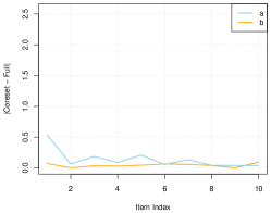
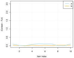
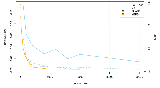
Figure 9: 2PL Experiments on real world SHARE (Börsch-Supan,, 2022) and NEPS data (NEPS-Network,, 2021): A comparison between the coreset sizes and the the quality of the solution found, by the relative error and the mean absolute deviation ($\alpha$), cf. Table 4. Let $f_{\sf full}$ and $f_{{\sf core}(j)}$ be the optimal values of the loss function on the input and on the coreset for the $j$-th repetition, respectively. Let $f_{\sf core}=\min_{j}f_{{\sf core}(j)}$. Relative error: rel. error $\hat{\varepsilon}=|f_{\sf core}-f_{\sf full}|/f_{\sf full}$ (cf. Lemma A.26). Mean Absolute Deviation: $\textbf{mad}(\alpha)=\frac{1}{n}\sum(|a_{\text{full}}-a_{\text{core}}|+|b_{\text{full}}-b_{\text{core}}|)$, evaluated on the parameters that attained the optimal $f_{\sf full}$ and $f_{\sf core}$. The coreset sizes for the NEPS data end at $10\,000$, to not exceed the input data size.

See Tables 2, 3, 5, 4, 6 and 7 and Figures 4, 5, 6, 7, 8, 9, 10, 11, 12 and 13 for additional experimental results on the parameter estimation accuracy along with the results already reported in the main paper.

Table 2: 2PL Experiments on synthetic data: The means and standard deviations (std.) of running times, taken across $20$ repetitions. In each repetition, the running time (in minutes) of 50 iterations of the main loop was measured per data set, and for different configurations of the data dimensions: the number of items $m$, the number of examinees $n$, and the coreset size $k$. The (relative) gain is defined as $(1-\mathrm{mean}_{\sf coreset}/\mathrm{mean}_{\sf full})\cdot 100$ %. The largest experiment was run only once, due to the large running time. Some measures thus do not apply, indicated by N/A values in the last row.

				Full data (min)		Coresets (min)
data	$\mathbf{n}$	$\mathbf{m}$	$\mathbf{k}$	mean	std.	mean	std.	gain
2PL-Syn	$50\,000$	$100$	$100$	$34.565$	$5.220$	$22.752$	$3.692$	$34.178$ %
2PL-Syn	$50\,000$	$200$	$500$	$65.745$	$11.897$	$30.121$	$4.645$	$54.185$ %
2PL-Syn	$50\,000$	$500$	$500$	$136.981$	$12.556$	$45.547$	$3.863$	$66.749$ %
2PL-Syn	$100\,000$	$100$	$100$	$75.135$	$11.881$	$51.029$	$7.524$	$32.084$ %
2PL-Syn	$100\,000$	$200$	$1\,000$	$122.252$	$12.043$	$61.459$	$10.654$	$49.727$ %
2PL-Syn	$100\,000$	$500$	$1\,000$	$231.276$	$23.793$	$80.861$	$11.161$	$65.037$ %
2PL-Syn	$200\,000$	$100$	$1\,000$	$155.053$	$18.877$	$99.352$	$12.055$	$35.924$ %
2PL-Syn	$200\,000$	$200$	$2\,000$	$247.654$	$34.069$	$119.075$	$13.717$	$51.919$ %
2PL-Syn	$200\,000$	$500$	$2\,000$	$466.832$	$48.734$	$169.494$	$21.862$	$63.693$ %
2PL-Syn	$500\,000$	$100$	$5\,000$	$339.057$	$115.382$	$228.041$	$75.920$	$32.743$ %
2PL-Syn	$500\,000$	$200$	$5\,000$	$518.274$	$77.108$	$291.678$	$44.327$	$43.721$ %
2PL-Syn	$500\,000$	$500$	$5\,000$	$1\,278.845$	$494.938$	$591.878$	$221.218$	$53.718$ %
2PL-Syn	$500\,000$	$5\,000$	$5\,000$	$9\,363.750$	N/A	$5\,536.684$	N/A	$40.871$ %

Table 3: 2PL Experiments on synthetic data: The quality of the solution found. Let $f_{\sf full}$ and $f_{{\sf core}(j)}$ be the optimal values of the loss function on the input and on the coreset for the $j$-th repetition, respectively. Let $f_{\sf core}=\min_{j}f_{{\sf core}(j)}$. Mean and standard deviation of the relative deviation $|f_{\sf core}-f_{{\sf core}(j)}|/f_{\sf core}$ (in $\%$): mean dev and std. dev. Relative error: rel. error $\hat{\varepsilon}=|f_{\sf core}-f_{\sf full}|/f_{\sf full}$ (cf. Lemma A.26). Mean Absolute Deviation: $\textbf{mad}(\alpha)=\frac{1}{n}\sum(|a_{\sf full}-a_{\sf core}|+|b_{\sf full}-b_{\sf core}|)$; $\textbf{mad}(\theta)=\frac{1}{m}\sum|\theta_{\sf full}-\theta_{\sf core}|$, evaluated on the parameters that attained the optimal $f_{\sf full}$ and $f_{\sf core}$. The largest experiment was run only once, due to the large running time. Some measures thus do not apply, indicated by N/A in the last row.

data	$\mathbf{n}$	$\mathbf{m}$	$\mathbf{k}$	mean dev	std. dev	rel. error $\hat{\varepsilon}$	$\text{mad}(\alpha)$	$\text{mad}(\theta)$
2PL-Syn	$50\,000$	$100$	$100$	$6.146$ %	$2.178$ %	$0.13452$	$1.108$	$0.045$
2PL-Syn	$50\,000$	$200$	$500$	$2.241$ %	$0.918$ %	$0.05214$	$0.508$	$0.011$
2PL-Syn	$50\,000$	$500$	$500$	$1.533$ %	$0.892$ %	$0.04803$	$0.525$	$0.008$
2PL-Syn	$100\,000$	$100$	$100$	$7.203$ %	$2.918$ %	$0.14776$	$0.970$	$0.040$
2PL-Syn	$100\,000$	$200$	$1\,000$	$1.086$ %	$0.544$ %	$0.03404$	$0.379$	$0.008$
2PL-Syn	$100\,000$	$500$	$1\,000$	$0.999$ %	$0.542$ %	$0.03140$	$0.345$	$0.005$
2PL-Syn	$200\,000$	$100$	$1\,000$	$1.936$ %	$0.849$ %	$0.04400$	$0.374$	$0.008$
2PL-Syn	$200\,000$	$200$	$2\,000$	$0.743$ %	$0.411$ %	$0.02375$	$0.248$	$0.003$
2PL-Syn	$200\,000$	$500$	$2\,000$	$1.273$ %	$0.565$ %	$0.03013$	$0.268$	$0.002$
2PL-Syn	$500\,000$	$100$	$5\,000$	$0.551$ %	$0.184$ %	$0.01399$	$0.142$	$0.002$
2PL-Syn	$500\,000$	$200$	$5\,000$	$0.731$ %	$0.275$ %	$0.01689$	$0.180$	$0.002$
2PL-Syn	$500\,000$	$500$	$5\,000$	$0.473$ %	$0.239$ %	$0.01445$	$0.171$	$0.001$
2PL-Syn	$500\,000$	$5\,000$	$5\,000$	N/A	N/A	$0.00076$	$0.120$	$0.013$

Figure 4: 2PL Experiments on synthetic data: Parameter estimates for the coresets compared to the full data sets. For each experiment the upper figure shows the bias for the item parameters $a$ and $b$. The lower figure shows a kernel density estimate for the ability parameters $\theta$ with a LOESS regression line in dark green. The ability parameters were standardized to zero mean and unit variance. In all rows, the vertical axis is scaled such as to display $2\,{\mathrm{std.}}$ of the corresponding parameter estimate obtained from the full data set.

$\mathbf{n=50\,000,m=100,k=100}$	$\mathbf{n=50\,000,m=200,k=500}$	$\mathbf{n=50\,000,m=500,k=500}$
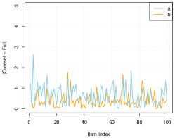
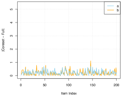
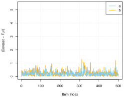
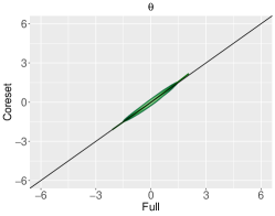
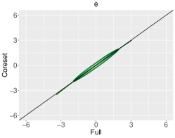
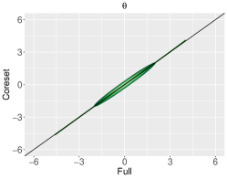
$\mathbf{n=100\,000,m=500,k=500}$	$\mathbf{n=100\,000,m=200,k=1\,000}$	$\mathbf{n=100\,000,m=500,k=1\,000}$

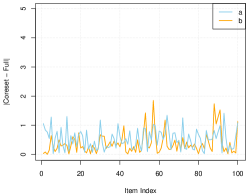
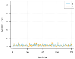
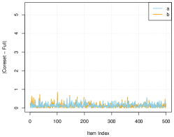
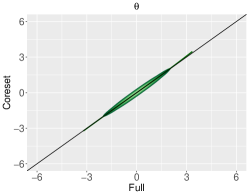
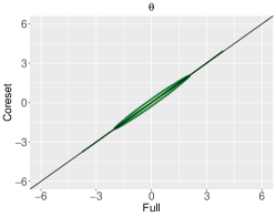
Figure 5: 2PL Experiments on synthetic data: Parameter estimates for the coresets compared to the full data sets. For each experiment the upper figure shows the bias for the item parameters $a$ and $b$. The lower figure shows a kernel density estimate for the ability parameters $\theta$ with a LOESS regression line in dark green. The ability parameters were standardized to zero mean and unit variance. In all rows, the vertical axis is scaled such as to display $2\,{\mathrm{std.}}$ of the corresponding parameter estimate obtained from the full data set.

$\mathbf{n=200\,000,m=100,k=1\,000}$	$\mathbf{n=200\,000,m=200,k=2\,000}$	$\mathbf{n=200\,000,m=500,k=2\,000}$
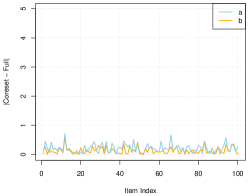
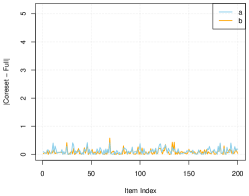
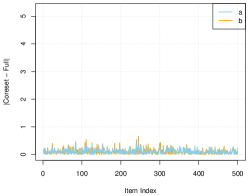
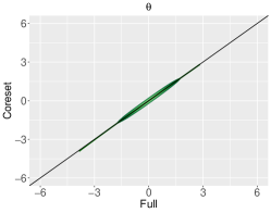
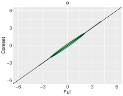
$\mathbf{n=500\,000,m=100,k=5\,000}$	$\mathbf{n=500\,000,m=200,k=5\,000}$	$\mathbf{n=500\,000,m=500,k=5\,000}$

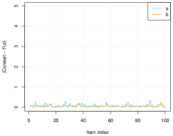
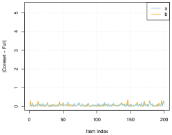
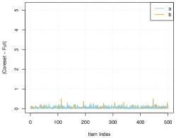
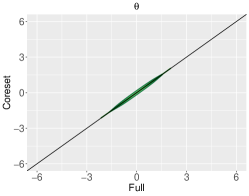
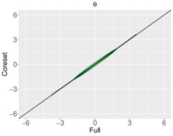
Figure 6: 2PL Experiments on synthetic data: Parameter estimates for the coresets compared to the full data set on the largest generated set with $n=500\,000$ and $m=5\,000$. For the experiment the left figure shows the bias for the item parameters $a$ and $b$. The right figure shows a kernel density estimate for the ability parameters $\theta$ with a LOESS regression line in dark green. The ability parameters were standardized to zero mean and unit variance. The vertical axis is scaled such as to display $2\,{\mathrm{std.}}$ of the corresponding parameter estimate obtained from the full data set.

$\mathbf{n=500\,000,m=5\,000,k=5\,000}$

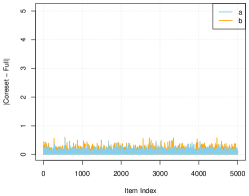
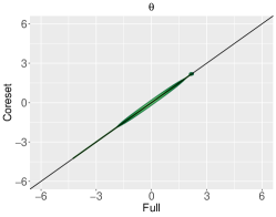
Table 4: 2PL Experiments on real world SHARE (Börsch-Supan,, 2022) and NEPS (NEPS-Network,, 2021) data: The quality of the solution found. Let $f_{\sf full}$ and $f_{{\sf core}(j)}$ be the optimal values of the loss function on the input and on the coreset for the $j$-th repetition, respectively. Let $f_{\sf core}=\min_{j}f_{{\sf core}(j)}$. Mean and standard deviation of the relative deviation $|f_{\sf core}-f_{{\sf core}(j)}|/f_{\sf core}$ (in $\%$): mean dev and std. dev. Relative error: rel. error $\hat{\varepsilon}=|f_{\sf core}-f_{\sf full}|/f_{\sf full}$ (cf. Lemma A.26). Mean Absolute Deviation: $\textbf{mad}(\alpha)=\frac{1}{n}\sum(|a_{\sf full}-a_{\sf core}|+|b_{\sf full}-b_{\sf core}|)$; $\textbf{mad}(\theta)=\frac{1}{m}\sum|\theta_{\sf full}-\theta_{\sf core}|$, evaluated on the parameters that attained the optimal $f_{\sf full}$ and $f_{\sf core}$.

data	$\mathbf{n}$	$\mathbf{m}$	$\mathbf{k}$	mean dev	std. dev	rel. error $\hat{\varepsilon}$	$\text{mad}(\alpha)$	$\text{mad}(\theta)$
SHARE	$138\,997$	$10$	$500$	$5.335$ %	$2.098$ %	$0.11347$	$0.770$	$0.090$
SHARE	$138\,997$	$10$	$1\,000$	$1.682$ %	$0.930$ %	$0.06193$	$0.307$	$0.040$
SHARE	$138\,997$	$10$	$2\,000$	$1.251$ %	$0.820$ %	$0.04263$	$0.129$	$0.015$
SHARE	$138\,997$	$10$	$4\,000$	$0.686$ %	$0.414$ %	$0.02791$	$0.108$	$0.013$
SHARE	$138\,997$	$10$	$6\,000$	$1.930$ %	$0.611$ %	$0.03546$	$0.095$	$0.007$
SHARE	$138\,997$	$10$	$8\,000$	$0.600$ %	$0.252$ %	$0.01935$	$0.061$	$0.007$
SHARE	$138\,997$	$10$	$10\,000$	$1.557$ %	$0.407$ %	$0.02713$	$0.092$	$0.014$
SHARE	$138\,997$	$10$	$20\,000$	$0.356$ %	$0.168$ %	$0.01415$	$0.045$	$0.003$
NEPS	$11\,532$	$88$	$100$	$4.363$ %	$2.176$ %	$0.09335$	$1.477$	$0.171$
NEPS	$11\,532$	$88$	$200$	$3.324$ %	$1.480$ %	$0.07134$	$0.930$	$0.142$
NEPS	$11\,532$	$88$	$500$	$1.969$ %	$0.657$ %	$0.03795$	$0.499$	$0.075$
NEPS	$11\,532$	$88$	$750$	$1.478$ %	$0.524$ %	$0.02675$	$0.432$	$0.062$
NEPS	$11\,532$	$88$	$1\,000$	$1.191$ %	$0.395$ %	$0.02007$	$0.320$	$0.045$
NEPS	$11\,532$	$88$	$2\,000$	$0.352$ %	$0.120$ %	$0.00506$	$0.182$	$0.026$
NEPS	$11\,532$	$88$	$5\,000$	$0.220$ %	$0.169$ %	$0.00147$	$0.101$	$0.015$
NEPS	$11\,532$	$88$	$10\,000$	$0.301$ %	$0.200$ %	$0.00094$	$0.071$	$0.012$

Table 5: 2PL Experiments on real world SHARE (Börsch-Supan,, 2022) and NEPS (NEPS-Network,, 2021) data: The means and standard deviations (std.) of running times, taken across $20$ repetitions. In each repetition, the running time (in minutes) of 50 iterations of the main loop was measured per data set for different configurations of the data dimensions: the number of items $m$, the number of examinees $n$, and the coreset size $k$. The (relative) gain is defined as $(1-\mathrm{mean}_{\mathrm{coreset}}/\mathrm{mean}_{\mathrm{full}})\cdot 100$ %.

				Full data (min)		Coresets (min)
data	$\mathbf{n}$	$\mathbf{m}$	$\mathbf{k}$	mean	std.	mean	std.	gain
SHARE	$138\,997$	$10$	$500$	$28.853$	$1.618$	$30.436$	$1.451$	$-5.484$ %
SHARE	$138\,997$	$10$	$1\,000$	$28.853$	$1.618$	$29.649$	$1.375$	$-2.758$ %
SHARE	$138\,997$	$10$	$2\,000$	$28.853$	$1.618$	$28.578$	$0.195$	$0.953$ %
SHARE	$138\,997$	$10$	$4\,000$	$28.853$	$1.618$	$27.861$	$0.070$	$3.439$ %
SHARE	$138\,997$	$10$	$6\,000$	$28.853$	$1.618$	$27.746$	$0.080$	$3.837$ %
SHARE	$138\,997$	$10$	$8\,000$	$28.853$	$1.618$	$27.637$	$0.085$	$4.216$ %
SHARE	$138\,997$	$10$	$10\,000$	$28.853$	$1.618$	$27.560$	$0.082$	$4.481$ %
SHARE	$138\,997$	$10$	$20\,000$	$28.853$	$1.618$	$27.525$	$0.085$	$4.603$ %
NEPS	$11\,532$	$88$	$100$	$5.968$	$0.061$	$4.020$	$0.010$	$32.640$ %
NEPS	$11\,532$	$88$	$200$	$5.968$	$0.061$	$4.113$	$0.257$	$31.084$ %
NEPS	$11\,532$	$88$	$500$	$5.968$	$0.061$	$4.402$	$0.333$	$26.237$ %
NEPS	$11\,532$	$88$	$750$	$5.968$	$0.061$	$4.036$	$0.014$	$32.373$ %
NEPS	$11\,532$	$88$	$1\,000$	$5.968$	$0.061$	$4.009$	$0.016$	$32.829$ %
NEPS	$11\,532$	$88$	$2\,000$	$5.968$	$0.061$	$3.940$	$0.057$	$33.983$ %
NEPS	$11\,532$	$88$	$5\,000$	$5.968$	$0.061$	$4.779$	$0.105$	$19.920$ %
NEPS	$11\,532$	$88$	$10\,000$	$5.968$	$0.061$	$5.849$	$0.064$	$2.003$ %

Figure 7: 2PL Experiments on the real world SHARE data (Börsch-Supan,, 2022). Parameter estimates for the coresets compared to the full data sets. For each experiment the upper figure shows the bias for the item parameters $a$ and $b$. The lower figure shows a kernel density estimate for the ability parameters $\theta$ with a LOESS regression line in dark green. The ability parameters were standardized to zero mean and unit variance. In all rows, the vertical axis is scaled such as to display $2\,{\mathrm{std.}}$ of the corresponding parameter estimate obtained from the full data set.

$\mathbf{n=138\,997,m=10,k=500}$	$\mathbf{n=138\,997,m=10,k=1\,000}$	$\mathbf{n=138\,997,m=10,k=2\,000}$

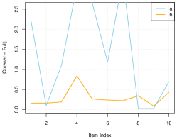
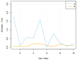
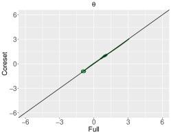
Figure 8: 2PL Experiments on the real world SHARE data (Börsch-Supan,, 2022). Parameter estimates for the coresets compared to the full data sets. For each experiment the upper figure shows the bias for the item parameters $a$ and $b$. The lower figure shows a kernel density estimate for the ability parameters $\theta$ with a LOESS regression line in dark green. The ability parameters were standardized to zero mean and unit variance. In all rows, the vertical axis is scaled such as to display $2\,{\mathrm{std.}}$ of the corresponding parameter estimate obtained from the full data set.

$\mathbf{n=138\,997,m=10,k=4\,000}$	$\mathbf{n=138\,997,m=10,k=6\,000}$	$\mathbf{n=138\,997,m=10,k=8\,000}$
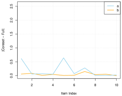
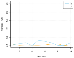
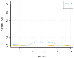
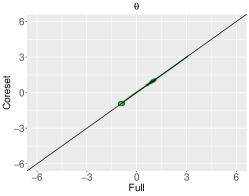
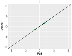
$\mathbf{n=138\,997,m=10,k=10\,000}$	$\mathbf{n=138\,997,m=10,k=20\,000}$

Figure 10: 2PL Experiments on real world NEPS data (NEPS-Network,, 2021): Parameter estimates for the coresets compared to the full data sets. For each experiment the upper figure shows the bias for the item parameters $a$ and $b$. The lower figure shows a kernel density estimate for the ability parameters $\theta$ with a LOESS regression line in dark green. The ability parameters were standardized to zero mean and unit variance. In all rows, the vertical axis is scaled such as to display $2\,{\mathrm{std.}}$ of the corresponding parameter estimate obtained from the full data set.

$\mathbf{n=11\,532,m=88,k=100}$	$\mathbf{n=11\,532,m=88,k=200}$	$\mathbf{n=11\,532,m=88,k=500}$

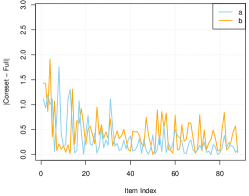
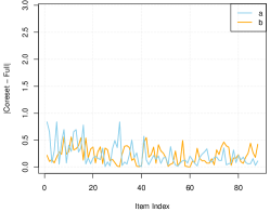
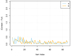
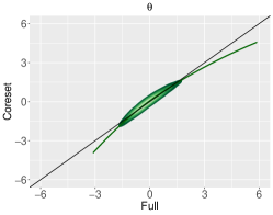
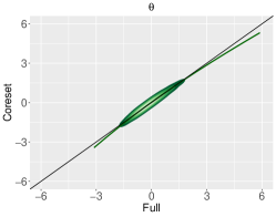
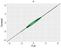
Figure 11: 2PL Experiments on real world NEPS data (NEPS-Network,, 2021): Parameter estimates for the coresets compared to the full data sets. For each experiment the upper figure shows the bias for the item parameters $a$ and $b$. The lower figure shows a kernel density estimate for the ability parameters $\theta$ with a LOESS regression line in dark green. The ability parameters were standardized to zero mean and unit variance. In all rows, the vertical axis is scaled such as to display $2\,{\mathrm{std.}}$ of the corresponding parameter estimate obtained from the full data set.

$\mathbf{n=11\,532,m=88,k=750}$	$\mathbf{n=11\,532,m=88,k=1\,000}$	$\mathbf{n=11\,532,m=88,k=2\,000}$
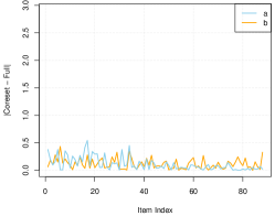
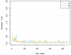
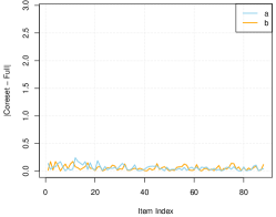
$\mathbf{n=11\,532,m=88,k=5\,000}$	$\mathbf{n=11\,532,m=88,k=10\,000}$

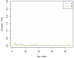
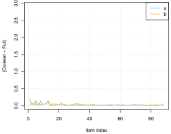
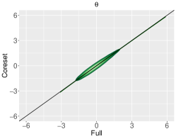
Table 6: 3PL Experiments on synthetic data: The means and standard deviations (std.) of running times, taken across $20$ repetitions. In each repetition, the running time (in minutes) of 50 iterations of the main loop was measured per data set for different configurations of the data dimensions: the number of items $m$, the number of examinees $n$, and the coreset size $k$. The (relative) gain is defined as $(1-\mathrm{mean}_{\sf coreset}/\mathrm{mean}_{\sf full})\cdot 100$ %.

				Full data (min)		Coresets (min)
data	$\mathbf{n}$	$\mathbf{m}$	$\mathbf{k}$	mean	std.	mean	std.	gain
3PL-Syn	$50\,000$	$100$	$2\,000$	$211.468$	$31.355$	$41.648$	$5.197$	$80.305$ %
3PL-Syn	$50\,000$	$100$	$5\,000$	$211.468$	$31.355$	$90.243$	$12.134$	$57.325$ %
3PL-Syn	$50\,000$	$100$	$10\,000$	$211.468$	$31.355$	$93.780$	$13.929$	$55.653$ %
3PL-Syn	$50\,000$	$200$	$2\,000$	$369.816$	$36.676$	$50.588$	$1.962$	$86.321$ %
3PL-Syn	$50\,000$	$200$	$5\,000$	$369.816$	$36.676$	$89.274$	$30.368$	$75.860$ %
3PL-Syn	$50\,000$	$200$	$10\,000$	$369.816$	$36.676$	$145.674$	$25.702$	$60.609$ %
3PL-Syn	$100\,000$	$100$	$5\,000$	$412.616$	$65.389$	$125.407$	$15.408$	$69.607$ %
3PL-Syn	$100\,000$	$200$	$5\,000$	$722.319$	$118.262$	$150.164$	$26.767$	$79.211$ %
3PL-Syn	$200\,000$	$100$	$10\,000$	$893.183$	$112.257$	$196.802$	$14.608$	$77.966$ %

Table 7: 3PL Experiments on synthetic data: The quality of the solution found. Let $f_{\sf full}$ and $f_{{\sf core}(j)}$ be the optimal values of the loss function on the input and on the coreset for the $j$-th repetition, respectively. Let $f_{\sf core}=\min_{j}f_{{\sf core}(j)}$. Mean and standard deviation of the relative deviation $|f_{\sf core}-f_{{\sf core}(j)}|/f_{\sf core}$ (in $\%$): mean dev and std. dev. Relative error: rel. error $\hat{\varepsilon}=|f_{\sf core}-f_{\sf full}|/f_{\sf full}$ (cf. Lemma A.26). Mean Absolute Deviation: $\textbf{mad}(\alpha)=\frac{1}{n}\sum(|a_{\sf full}-a_{\sf core}|+|b_{\sf full}-b_{\sf core}|+|c_{\sf full}-c_{\sf core}|)$; $\textbf{mad}(\theta)=\frac{1}{m}\sum|\theta_{\sf full}-\theta_{\sf core}|$, evaluated on the parameters that attained the optimal $f_{\sf full}$ and $f_{\sf core}$.

data	$\mathbf{n}$	$\mathbf{m}$	$\mathbf{k}$	mean dev	std. dev	rel. error $\hat{\varepsilon}$	$\text{mad}(\alpha)$	$\text{mad}(\theta)$
3PL-Syn	$50\,000$	$100$	$2\,000$	$4.495$ %	$2.392$ %	$0.45212$	$2.820$	$0.625$
3PL-Syn	$50\,000$	$100$	$5\,000$	$2.061$ %	$1.935$ %	$0.03228$	$0.968$	$0.048$
3PL-Syn	$50\,000$	$100$	$10\,000$	$2.237$ %	$2.417$ %	$0.00212$	$0.384$	$0.010$
3PL-Syn	$50\,000$	$200$	$2\,000$	$5.280$ %	$3.065$ %	$0.43784$	$2.832$	$0.649$
3PL-Syn	$50\,000$	$200$	$5\,000$	$4.536$ %	$2.615$ %	$0.01662$	$0.906$	$0.037$
3PL-Syn	$50\,000$	$200$	$10\,000$	$3.306$ %	$1.459$ %	$0.02186$	$0.488$	$0.001$
3PL-Syn	$100\,000$	$100$	$5\,000$	$8.370$ %	$3.944$ %	$0.02065$	$1.375$	$0.101$
3PL-Syn	$100\,000$	$200$	$5\,000$	$4.819$ %	$1.784$ %	$0.06281$	$1.545$	$0.140$
3PL-Syn	$200\,000$	$100$	$10\,000$	$3.413$ %	$2.529$ %	$0.01789$	$0.524$	$0.003$

Figure 12: 3PL Experiments on synthetic data. Parameter estimates for the coresets compared to the full data sets. For each experiment the upper figure shows the bias for the item parameters $a$ and $b$. The lower figure shows a kernel density estimate for the ability parameters $\theta$ with a LOESS regression line in dark green. The ability parameters were standardized to zero mean and unit variance. In all rows, the vertical axis is scaled such as to display $4\,{\mathrm{std.}}$ of the corresponding parameter estimate obtained from the full data set.

$\mathbf{n=50\,000,m=100,k=2\,000}$	$\mathbf{n=50\,000,m=100,k=5\,000}$	$\mathbf{n=50\,000,m=100,k=10\,000}$
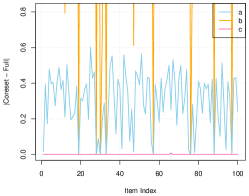
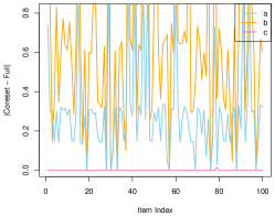
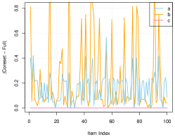
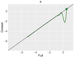
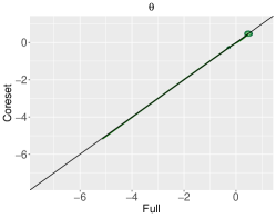
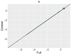
$\mathbf{n=50\,000,m=200,k=2\,000}$	$\mathbf{n=50\,000,m=200,k=5\,000}$	$\mathbf{n=50\,000,m=200,k=10\,000}$

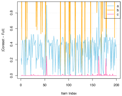
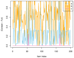
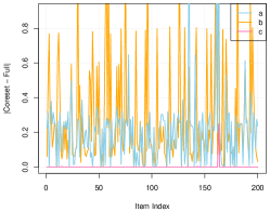
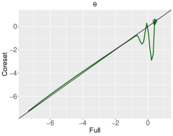
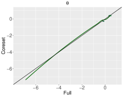
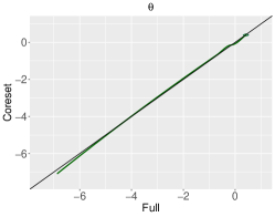
Figure 13: 3PL Experiments on synthetic data. Parameter estimates for the coresets compared to the full data sets. For each experiment the upper figure shows the bias for the item parameters $a$ and $b$. The lower figure shows a kernel density estimate for the ability parameters $\theta$ with a LOESS regression line in dark green. The ability parameters were standardized to zero mean and unit variance. In all rows, the vertical axis is scaled such as to display $4\,{\mathrm{std.}}$ of the corresponding parameter estimate obtained from the full data set.

$\mathbf{n=100\,000,m=100,k=5\,000}$	$\mathbf{n=100\,000,m=200,k=5\,000}$	$\mathbf{n=200\,000,m=100,k=10\,000}$

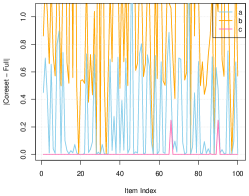
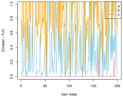
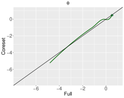
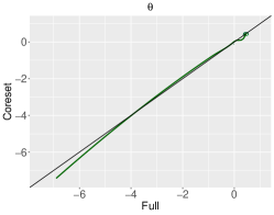
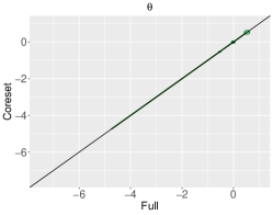
Appendix C COMPARISON TO UNIFORM SAMPLING

The interested reader may ask why not to simply use uniformly sampled subsets of the input instead of coresets, as this is arguably the de facto standard baseline used for estimating IRT models from subsamples. For instance, Karadavut, (2016) showed in an extensive comparison that uniform sampling works better than standard $\ell_{2}$-leverage score methods (note that we use square root $\ell_{2}$-leverage scores, which makes a large difference). Further, uniform sampling is commonly used for constructing training data by subsampling from the complete data space $\{-1,1\}^{m\times n}$ (Bonifay and Cai,, 2017).

However, it is well known that uniform samples of sublinear size cannot yield strong multiplicative approximation guarantees, even for mild data with $\mu=1$. This also holds for other techniques that rely on uniform subsampling, such as stochastic gradient descent (SGD) as the authors demonstrate theoretically, and practically in (Munteanu et al.,, 2018). Coresets, in contrast, are designed to provably approximate the loss to within a $(1+\varepsilon)$ factor with sublinear sample size in the natural case where $\mu$ is bounded.

To corroborate this in the context of IRT models, we compared between the approximation achieved by uniformly sampled subsets of the input and our coresets, after 50 iterations for 2PL IRT models on synthetic data (generated as described in the main body) and on real-world SHARE (Börsch-Supan,, 2022) and NEPS data (NEPS-Network,, 2021). The results are measured for both methods in terms of mean absolute deviations of calculated estimates from the actual item parameters and from the actual ability parameter, as well in terms of the relative error of the objective function, cf. Lemma A.26, summarized in Tables 8, 9 and 10.

Initial experiments showed that the uniform samples were consistently less accurate by (at least) one order of magnitude regarding the Mean Absolute Deviation (MAD). To get an impression of the best performance of the two methods, we repeat both experiments using uniform samples and the coresets 20 times independently and compare the best result for each method to one another. Note that the information on which repetition gave the best result is not available in practice, so this is an overly optimistic scenario.

Indeed, for the best performing repetition, the parameter estimates from uniform samples w.r.t MAD are comparable up to a negligible amount. But the relative error of the objective function approximation using uniform samples is very large. For the synthetic data, the relative error is always around $50\,\%$, while for the real-world data, we see that the error actually decreases as the data sample size grows. However, to get a result of comparable quality to the coresets, the uniform sample needs to comprise almost the whole input, while our coresets achieve the same error using a tiny fraction of the input (cf. Table 10).

We also note that downstream tasks, such as calculating gradients, uncertainty quantification measures, Hessian, Fisher information etc. require a close approximation of the objective function. We thus conclude that coresets are better suited than uniform sampling, even in optimistic situations where the latter yields accurate point estimation results.

Table 8: 2PL experiments on synthetic data for uniformly sampled subsets vs. coresets. Comparison of the best solutions found taken across $20$ repetitions (each running $50$ iterations of the main loop) per data set for different configurations of the data dimensions: the number of items $m$, the number of examinees $n$, and the uniform sample/coreset size $k$. Let $f_{\sf full}$, $f_{{\sf unif}(j)}$ and $f_{{\sf core}(j)}$ be the optimal values of the loss function on the input, on the uniform sample for the $j$-th repetition, and on the coreset for the $j$-th repetition, respectively. Let $f_{\sf unif}=\min_{j}f_{{\sf unif}(j)}$, and $f_{\sf core}=\min_{j}f_{{\sf core}(j)}$. Comparison made w.r.t. Relative errors: r.err. $\hat{\varepsilon}_{\sf unif}$$=|f_{\sf unif}-f_{\sf full}|/f_{\sf full}$, r.err. $\hat{\varepsilon}_{\sf core}$$=|f_{\sf core}-f_{\sf full}|/f_{\sf full}$ (cf. Lemma A.26), and Mean Absolute Deviations (MAD): $\text{mad}_{\sf core}(\alpha)=\frac{1}{n}\sum(|a_{\sf full}-a_{\sf core}|+|b_{\sf full}-b_{\sf core}|)$; $\text{mad}_{\sf core}(\theta)=\frac{1}{m}\sum|\theta_{\sf full}-\theta_{\sf core}|$. $\text{mad}_{\sf unif}(\alpha)=\frac{1}{n}\sum(|a_{\sf full}-a_{\sf unif}|+|b_{\sf full}-b_{\sf unif}|)$; $\text{mad}_{\sf unif}(\theta)=\frac{1}{m}\sum|\theta_{\sf full}-\theta_{\sf unif}|$.

			Uniform sampling			Coresets
$\mathbf{n}$	$\mathbf{m}$	$\mathbf{k}$	$\text{mad}_{\sf unif}(\alpha)$	$\text{mad}_{\sf unif}(\theta)$	r.err. $\hat{\varepsilon}_{\sf unif}$	$\text{mad}_{\sf core}(\alpha)$	$\text{mad}_{\sf core}(\theta)$	r.err. $\hat{\varepsilon}_{\sf core}$
$50\,000$	$100$	$100$	$1.023$	$0.029$	$0.49127$	$1.108$	$0.045$	$0.13452$
$50\,000$	$200$	$500$	$0.475$	$0.009$	$0.49284$	$0.508$	$0.011$	$0.05214$
$50\,000$	$500$	$500$	$0.450$	$0.004$	$0.49262$	$0.525$	$0.008$	$0.04803$
$100\,000$	$100$	$100$	$0.975$	$0.077$	$0.49173$	$0.970$	$0.040$	$0.14776$
$100\,000$	$200$	$1\,000$	$0.318$	$0.007$	$0.49389$	$0.379$	$0.008$	$0.03404$
$100\,000$	$500$	$1\,000$	$0.351$	$0.002$	$0.49377$	$0.345$	$0.005$	$0.03140$
$200\,000$	$100$	$1\,000$	$0.331$	$0.005$	$0.49643$	$0.374$	$0.008$	$0.04400$
$200\,000$	$200$	$2\,000$	$0.241$	$0.003$	$0.49442$	$0.248$	$0.003$	$0.02375$
$200\,000$	$500$	$2\,000$	$0.239$	$0.002$	$0.49436$	$0.268$	$0.002$	$0.03013$
$500\,000$	$100$	$5\,000$	$0.146$	$0.002$	$0.49479$	$0.142$	$0.002$	$0.01399$
$500\,000$	$200$	$5\,000$	$0.157$	$0.002$	$0.49478$	$0.180$	$0.002$	$0.01689$
$500\,000$	$500$	$5\,000$	$0.167$	$0.001$	$0.49477$	$0.171$	$0.001$	$0.01445$

Table 9: 2PL experiments on real-world SHARE data (Börsch-Supan,, 2022) for uniformly sampled subsets vs. coresets. Comparison of the best solutions found taken across $20$ repetitions (each running $50$ iterations of the main loop) per data set for different configurations of the data dimensions: the number of items $m$, the number of examinees $n$, and the uniform sample/coreset size $k$. Let $f_{\sf full}$, $f_{{\sf unif}(j)}$ and $f_{{\sf core}(j)}$ be the optimal values of the loss function on the input, on the uniform sample for the $j$-th repetition, and on the coreset for the $j$-th repetition, respectively. Let $f_{\sf unif}=\min_{j}f_{{\sf unif}(j)}$, and $f_{\sf core}=\min_{j}f_{{\sf core}(j)}$. Comparison made w.r.t. Relative errors: r.err. $\hat{\varepsilon}_{\sf unif}$$=|f_{\sf unif}-f_{\sf full}|/f_{\sf full}$, r.err. $\hat{\varepsilon}_{\sf core}$$=|f_{\sf core}-f_{\sf full}|/f_{\sf full}$ (cf. Lemma A.26), and Mean Absolute Deviations (MAD): $\text{mad}_{\sf core}(\alpha)=\frac{1}{n}\sum(|a_{\sf full}-a_{\sf core}|+|b_{\sf full}-b_{\sf core}|)$; $\text{mad}_{\sf core}(\theta)=\frac{1}{m}\sum|\theta_{\sf full}-\theta_{\sf core}|$. $\text{mad}_{\sf unif}(\alpha)=\frac{1}{n}\sum(|a_{\sf full}-a_{\sf unif}|+|b_{\sf full}-b_{\sf unif}|)$; $\text{mad}_{\sf unif}(\theta)=\frac{1}{m}\sum|\theta_{\sf full}-\theta_{\sf unif}|$.

			Uniform sampling			Coresets
$\mathbf{n}$	$\mathbf{m}$	$\mathbf{k}$	$\text{mad}_{\sf unif}(\alpha)$	$\text{mad}_{\sf unif}(\theta)$	r.err. $\hat{\varepsilon}_{\sf unif}$	$\text{mad}_{\sf core}(\alpha)$	$\text{mad}_{\sf core}(\theta)$	r.err. $\hat{\varepsilon}_{\sf core}$
$138\,997$	$10$	$500$	$0.722$	$0.071$	$0.49618$	$0.770$	$0.090$	$0.11347$
$138\,997$	$10$	$1\,000$	$0.232$	$0.034$	$0.49534$	$0.307$	$0.040$	$0.06193$
$138\,997$	$10$	$2\,000$	$0.179$	$0.020$	$0.49255$	$0.129$	$0.015$	$0.04263$
$138\,997$	$10$	$4\,000$	$0.083$	$0.004$	$0.48608$	$0.108$	$0.013$	$0.02791$
$138\,997$	$10$	$6\,000$	$0.086$	$0.005$	$0.47939$	$0.095$	$0.007$	$0.03546$
$138\,997$	$10$	$8\,000$	$0.082$	$0.006$	$0.47202$	$0.061$	$0.007$	$0.01935$
$138\,997$	$10$	$10\,000$	$0.059$	$0.008$	$0.46502$	$0.092$	$0.014$	$0.02713$
$138\,997$	$10$	$20\,000$	$0.058$	$0.010$	$0.42961$	$0.045$	$0.003$	$0.01415$

Table 10: 2PL experiments on real-world NEPS data (NEPS-Network,, 2021) for uniformly sampled subsets vs. coresets. Comparison of the best solutions found taken across $20$ repetitions (each running $50$ iterations of the main loop) per data set for different configurations of the data dimensions: the number of items $m$, the number of examinees $n$, and the uniform sample/coreset size $k$. Let $f_{\sf full}$, $f_{{\sf unif}(j)}$ and $f_{{\sf core}(j)}$ be the optimal values of the loss function on the input, on the uniform sample for the $j$-th repetition, and on the coreset for the $j$-th repetition, respectively. Let $f_{\sf unif}=\min_{j}f_{{\sf unif}(j)}$, and $f_{\sf core}=\min_{j}f_{{\sf core}(j)}$. Comparison made w.r.t. Relative errors: r.err. $\hat{\varepsilon}_{\sf unif}$$=|f_{\sf unif}-f_{\sf full}|/f_{\sf full}$, r.err. $\hat{\varepsilon}_{\sf core}$$=|f_{\sf core}-f_{\sf full}|/f_{\sf full}$ (cf. Lemma A.26), and Mean Absolute Deviations (MAD): $\text{mad}_{\sf core}(\alpha)=\frac{1}{n}\sum(|a_{\sf full}-a_{\sf core}|+|b_{\sf full}-b_{\sf core}|)$; $\text{mad}_{\sf core}(\theta)=\frac{1}{m}\sum|\theta_{\sf full}-\theta_{\sf core}|$. $\text{mad}_{\sf unif}(\alpha)=\frac{1}{n}\sum(|a_{\sf full}-a_{\sf unif}|+|b_{\sf full}-b_{\sf unif}|)$; $\text{mad}_{\sf unif}(\theta)=\frac{1}{m}\sum|\theta_{\sf full}-\theta_{\sf unif}|$.

			Uniform sampling			Coresets
$\mathbf{n}$	$\mathbf{m}$	$\mathbf{k}$	$\text{mad}_{\sf unif}(\alpha)$	$\text{mad}_{\sf unif}(\theta)$	r.err. $\hat{\varepsilon}_{\sf unif}$	$\text{mad}_{\sf core}(\alpha)$	$\text{mad}_{\sf core}(\theta)$	r.err. $\hat{\varepsilon}_{\sf core}$
$11\,532$	$88$	$100$	$1.561$	$0.185$	$0.48878$	$1.477$	$0.171$	$0.09335$
$11\,532$	$88$	$200$	$1.056$	$0.131$	$0.48762$	$0.930$	$0.142$	$0.07134$
$11\,532$	$88$	$500$	$0.635$	$0.096$	$0.47713$	$0.499$	$0.075$	$0.03795$
$11\,532$	$88$	$750$	$0.486$	$0.068$	$0.46702$	$0.432$	$0.062$	$0.02675$
$11\,532$	$88$	$1\,000$	$0.393$	$0.053$	$0.45664$	$0.320$	$0.045$	$0.02007$
$11\,532$	$88$	$2\,000$	$0.227$	$0.030$	$0.41390$	$0.182$	$0.026$	$0.00506$
$11\,532$	$88$	$5\,000$	$0.107$	$0.011$	$0.28429$	$0.101$	$0.015$	$0.00147$
$11\,532$	$88$	$10\,000$	$0.029$	$0.002$	$0.06711$	$0.071$	$0.012$	$0.00094$

Appendix D COMPARISON TO CORESETS FOR CLUSTERING

The interested reader may find that the alternating optimization algorithm resembles some kind of EM-type algorithm, akin to the popular Lloyd’s algorithm for the $k$-means clustering problem. One crucial difference, however, is that in the IRT context, both sets of parameters to be estimated are unknown latent variables, while for the $k$-means problem, one set of ’parameters’, is implicitly given by the data, and the task reduces to finding the other set (the $k$ cluster centers). We also note that in the IRT problem, the desired output is an explicit description of $m$ ability parameters, and $n$ item parameters. One can thus not hope to reduce one (or both) of the dimensions only once and work only on this single reduced coreset, as is possible for $k$-means.

Despite the above mentioned differences, the interested reader may ask why we should construct new coresets for the IRT models, if already existing solutions from a plethora of coresets designed for clustering problems would serve as well.

Recently, Schwiegelshohn and Sheikh-Omar, (2022) provided an extensive empirical comparison of various coreset constructions. The best performing coresets in practice were generated by ‘distance sampling’, which is based on sensitivity sampling (Feldman and Langberg,, 2011; Langberg and Schulman,, 2010), the same coreset design pattern that we also used for our coreset construction. In the case of clustering problems, first an initial (and rough) bi-criteria approximation is computed. Then, subsampling is performed proportionally to the squared Euclidean distance of input points to their closest center from this approximation. This coreset construction consistently outperformed all competitors in (Schwiegelshohn and Sheikh-Omar,, 2022), even the relatively new group sampling technique that achieves optimal theoretical bounds (Cohen-Addad et al.,, 2021).

Thus, we compare our coresets to the winning ‘distance sampling’ in terms of their approximation quality when applied to IRT models. The results are given in Tables 11, 12 and 13.

For all data sets, our coresets outperform the distance sampling coresets in terms of their approximation quality, for both, mean absolute deviation (MAD) and the relative error. The MAD obtained from distance sampling coresets is at least twice as large as the MAD on our coresets. The relative error of the distance sampling coresets is at least $20\,\%$ larger than using our coresets, sometimes as much as two or three times larger, or even worse on the real-world data sets. Indeed, on the real-world SHARE data set (Börsch-Supan,, 2022), which is very sparse, the distance sampling coresets cannot approximate the loss function well enough (the relative error remains $\hat{\varepsilon}>0.30$), even if we allow $72\,\%$ of the input ($100\,000$ examinees) to be selected into the coresets. In comparison, our coresets approximate the loss function up to relative error $\hat{\varepsilon}<0.03$ by taking a coreset that comprises only $6\,\%$ of the input set ($8\,000$ examinees). Our construction seems much more robust to this sparse data setting.

We conclude that the distance sampling coresets can in some settings provide good approximations that are competitive to our coresets, but their performance deteriorates in the presence of sparse data. Only coresets that are specifically tailored for IRT models provide an approximation of guaranteed quality.

Table 11: 2PL experiments on synthetic data for distance sampling coresets, based on sensitivity sampling, vs. IRT coresets. Comparison of the best solutions found taken across $10$ repetitions (each running $50$ iterations of the main loop) per data set for different configurations of the data dimensions: the number of items $m$, the number of examinees $n$, and the distance sample/coreset size $k$. Let $f_{\sf full}$, $f_{{\sf dist}(j)}$ and $f_{{\sf core}(j)}$ be the optimal values of the loss function on the input, on the distance sample for the $j$-th repetition, and on the coreset for the $j$-th repetition, respectively. Let $f_{\sf dist}=\min_{j}f_{{\sf dist}(j)}$, and $f_{\sf core}=\min_{j}f_{{\sf core}(j)}$. Comparison made w.r.t. Relative errors: r.err. $\hat{\varepsilon}_{\sf dist}$$=|f_{\sf dist}-f_{\sf full}|/f_{\sf full}$, r.err. $\hat{\varepsilon}_{\sf core}$$=|f_{\sf core}-f_{\sf full}|/f_{\sf full}$ (cf. Lemma A.26), and Mean Absolute Deviations (MAD): $\text{mad}_{\sf core}(\alpha)=\frac{1}{n}\sum(|a_{\sf full}-a_{\sf core}|+|b_{\sf full}-b_{\sf core}|)$; $\text{mad}_{\sf core}(\theta)=\frac{1}{m}\sum|\theta_{\sf full}-\theta_{\sf core}|$. $\text{mad}_{\sf dist}(\alpha)=\frac{1}{n}\sum(|a_{\sf full}-a_{\sf dist}|+|b_{\sf full}-b_{\sf dist}|)$; $\text{mad}_{\sf dist}(\theta)=\frac{1}{m}\sum|\theta_{\sf full}-\theta_{\sf dist}|$.

			Distance sampling coresets			IRT coresets
$\mathbf{n}$	$\mathbf{m}$	$\mathbf{k}$	$\textbf{mad}_{\sf dist}(\alpha)$	$\textbf{mad}_{\sf dist}(\theta)$	r.err. $\hat{\varepsilon}_{\sf dist}$	$\textbf{mad}_{\sf core}(\alpha)$	$\textbf{mad}_{\sf core}(\theta)$	r.err. $\hat{\varepsilon}_{\sf core}$
$50\,000$	$100$	$100$	$1.146$	$0.058$	$0.15496$	$1.108$	$0.045$	$0.13452$
$50\,000$	$200$	$500$	$0.659$	$0.013$	$0.08284$	$0.508$	$0.011$	$0.05214$
$50\,000$	$500$	$500$	$0.609$	$0.013$	$0.08582$	$0.525$	$0.008$	$0.04803$
$100\,000$	$100$	$100$	$1.149$	$0.027$	$0.14136$	$0.970$	$0.040$	$0.14776$
$100\,000$	$200$	$1\,000$	$0.760$	$0.009$	$0.05923$	$0.379$	$0.008$	$0.03404$
$100\,000$	$500$	$1\,000$	$0.448$	$0.011$	$0.07641$	$0.345$	$0.005$	$0.03140$
$200\,000$	$100$	$1\,000$	$0.543$	$0.022$	$0.06787$	$0.374$	$0.008$	$0.04400$
$200\,000$	$200$	$2\,000$	$0.343$	$0.005$	$0.04916$	$0.248$	$0.003$	$0.02375$
$200\,000$	$500$	$2\,000$	$0.354$	$0.005$	$0.04667$	$0.268$	$0.002$	$0.03013$
$500\,000$	$100$	$5\,000$	$0.252$	$0.013$	$0.03292$	$0.142$	$0.002$	$0.01399$
$500\,000$	$200$	$5\,000$	$0.295$	$0.005$	$0.03394$	$0.180$	$0.002$	$0.01689$
$500\,000$	$500$	$5\,000$	$0.259$	$0.003$	$0.03424$	$0.171$	$0.001$	$0.01445$

Table 12: 2PL experiments on real-world SHARE data for distance sampling coresets, based on sensitivity sampling, vs. IRT coresets. Comparison of the best solutions found taken across $10$ repetitions (each running $50$ iterations of the main loop) per data set for different configurations of the data dimensions: the number of items $m$, the number of examinees $n$, and the distance sample/coreset size $k$. Let $f_{\sf full}$, $f_{{\sf dist}(j)}$ and $f_{{\sf core}(j)}$ be the optimal values of the loss function on the input, on the distance sample for the $j$-th repetition, and on the coreset for the $j$-th repetition, respectively. Let $f_{\sf dist}=\min_{j}f_{{\sf dist}(j)}$, and $f_{\sf core}=\min_{j}f_{{\sf core}(j)}$. Comparison made w.r.t. Relative errors: r.err. $\hat{\varepsilon}_{\sf dist}$$=|f_{\sf dist}-f_{\sf full}|/f_{\sf full}$, r.err. $\hat{\varepsilon}_{\sf core}$$=|f_{\sf core}-f_{\sf full}|/f_{\sf full}$ (cf. Lemma A.26), and Mean Absolute Deviations (MAD): $\text{mad}_{\sf core}(\alpha)=\frac{1}{n}\sum(|a_{\sf full}-a_{\sf core}|+|b_{\sf full}-b_{\sf core}|)$; $\text{mad}_{\sf core}(\theta)=\frac{1}{m}\sum|\theta_{\sf full}-\theta_{\sf core}|$. $\text{mad}_{\sf dist}(\alpha)=\frac{1}{n}\sum(|a_{\sf full}-a_{\sf dist}|+|b_{\sf full}-b_{\sf dist}|)$; $\text{mad}_{\sf dist}(\theta)=\frac{1}{m}\sum|\theta_{\sf full}-\theta_{\sf dist}|$.

			Distance sampling coresets			IRT coresets
$\mathbf{n}$	$\mathbf{m}$	$\mathbf{k}$	$\textbf{mad}_{\sf dist}(\alpha)$	$\textbf{mad}_{\sf dist}(\theta)$	r.err. $\hat{\varepsilon}_{\sf dist}$	$\textbf{mad}_{\sf core}(\alpha)$	$\textbf{mad}_{\sf core}(\theta)$	$\hat{\varepsilon}_{\sf core}$
$138\,997$	$10$	$500$	$3.581$	$0.329$	$0.3843766731629$	$0.770$	$0.090$	$0.11347$
$138\,997$	$10$	$1\,000$	$3.580$	$0.328$	$0.3843766731630$	$0.307$	$0.040$	$0.06193$
$138\,997$	$10$	$2\,000$	$3.586$	$0.330$	$0.3843766731634$	$0.129$	$0.015$	$0.04263$
$138\,997$	$10$	$4\,000$	$3.579$	$0.328$	$0.3843766731618$	$0.108$	$0.013$	$0.02791$
$138\,997$	$10$	$6\,000$	$3.581$	$0.328$	$0.3843766731613$	$0.095$	$0.007$	$0.03546$
$138\,997$	$10$	$8\,000$	$3.580$	$0.328$	$0.3843766731606$	$0.061$	$0.007$	$0.01935$
$138\,997$	$10$	$10\,000$	$3.581$	$0.328$	$0.3843766731605$	$0.092$	$0.014$	$0.02713$
$138\,997$	$10$	$20\,000$	$3.580$	$0.328$	$0.3843766731608$	$0.045$	$0.003$	$0.01415$

Table 13: 2PL experiments on real-world NEPS data for distance sampling coresets, based on sensitivity sampling, vs. IRT coresets. Comparison of the best solutions found taken across $10$ repetitions (each running $50$ iterations of the main loop) per data set for different configurations of the data dimensions: the number of items $m$, the number of examinees $n$, and the distance sample/coreset size $k$. Let $f_{\sf full}$, $f_{{\sf dist}(j)}$ and $f_{{\sf core}(j)}$ be the optimal values of the loss function on the input, on the distance sample for the $j$-th repetition, and on the coreset for the $j$-th repetition, respectively. Let $f_{\sf dist}=\min_{j}f_{{\sf dist}(j)}$, and $f_{\sf core}=\min_{j}f_{{\sf core}(j)}$. Comparison made w.r.t. Relative errors: r.err. $\hat{\varepsilon}_{\sf dist}$$=|f_{\sf dist}-f_{\sf full}|/f_{\sf full}$, r.err. $\hat{\varepsilon}_{\sf core}$$=|f_{\sf core}-f_{\sf full}|/f_{\sf full}$ (cf. Lemma A.26), and Mean Absolute Deviations (MAD): $\text{mad}_{\sf core}(\alpha)=\frac{1}{n}\sum(|a_{\sf full}-a_{\sf core}|+|b_{\sf full}-b_{\sf core}|)$; $\text{mad}_{\sf core}(\theta)=\frac{1}{m}\sum|\theta_{\sf full}-\theta_{\sf core}|$. $\text{mad}_{\sf dist}(\alpha)=\frac{1}{n}\sum(|a_{\sf full}-a_{\sf dist}|+|b_{\sf full}-b_{\sf dist}|)$; $\text{mad}_{\sf dist}(\theta)=\frac{1}{m}\sum|\theta_{\sf full}-\theta_{\sf dist}|$.

			Distance sampling coresets			IRT coresets
$\mathbf{n}$	$\mathbf{m}$	$\mathbf{k}$	$\textbf{mad}_{\sf dist}(\alpha)$	$\textbf{mad}_{\sf dist}(\theta)$	r.err. $\hat{\varepsilon}_{\sf dist}$	$\textbf{mad}_{\sf core}(\alpha)$	$\textbf{mad}_{\sf core}(\theta)$	r.err. $\hat{\varepsilon}_{\sf core}$
$11\,532$	$88$	$100$	$2.244$	$0.433$	$0.12674$	$1.477$	$0.171$	$0.09335$
$11\,532$	$88$	$200$	$1.818$	$0.198$	$0.11617$	$0.930$	$0.142$	$0.07134$
$11\,532$	$88$	$500$	$0.959$	$0.138$	$0.07654$	$0.499$	$0.075$	$0.03795$
$11\,532$	$88$	$750$	$0.432$	$0.103$	$0.07988$	$0.432$	$0.062$	$0.02675$
$11\,532$	$88$	$1\,000$	$0.654$	$0.101$	$0.06035$	$0.320$	$0.045$	$0.02007$
$11\,532$	$88$	$2\,000$	$0.490$	$0.068$	$0.06295$	$0.182$	$0.026$	$0.00506$
$11\,532$	$88$	$5\,000$	$0.101$	$0.043$	$0.04319$	$0.101$	$0.015$	$0.00147$
$11\,532$	$88$	$10\,000$	$0.301$	$0.031$	$0.04802$	$0.071$	$0.012$	$0.00094$

Appendix E COMPARISON TO $\ell_{1}$ LEVERAGE SCORES AND $\ell_{1}$ LEWIS WEIGHTS

Further baselines for subsampling the input that are used in the literature to approximate the objective functions related to logistic regression, are sampling proportional to $\ell_{1}$-leverage scores (Munteanu et al.,, 2022), resp. to $\ell_{1}$-Lewis weights (Mai et al.,, 2021).

We compared our coresets to the $\ell_{1}$-leverage scores, resp. $\ell_{1}$-Lewis weights, in terms of their approximation quality, their mean absolute deviation (MAD) and their relative error.

Our IRT coresets show very similar, and often slightly better performance compared to both alternative subsampling techniques, when applied to the synthetic, and the real-world data instances for the 2PL IRT model.

See Tables 14, 15 and 16 below for the comparison of our coresets to sampling based on $\ell_{1}$-leverage scores. Also, see Tables 17, 18 and 19 below for the comparison of our coresets to sampling based on $\ell_{1}$-Lewis weights.

E.1 $\ell_{1}$-Leverage Score Sampling

Table 14: 2PL experiments on synthetic data for $\ell_{1}$-leverage score sampling coresets, vs. IRT coresets. Comparison of the best solutions found taken across $10$ repetitions (each running $50$ iterations of the main loop) per data set for different configurations of the data dimensions: the number of items $m$, the number of examinees $n$, and the $\ell_{1}$-leverage score sample/coreset size $k$. Let $f_{\sf full}$, $f_{{\sf L1s}(j)}$ and $f_{{\sf core}(j)}$ be the optimal values of the loss function on the input, on the distance sample for the $j$-th repetition, and on the coreset for the $j$-th repetition, respectively. Let $f_{\sf L1s}=\min_{j}f_{{\sf L1s}(j)}$, and $f_{\sf core}=\min_{j}f_{{\sf core}(j)}$. Comparison made w.r.t. Relative errors: r.err. $\hat{\varepsilon}_{\sf L1s}$$=|f_{\sf L1s}-f_{\sf full}|/f_{\sf full}$, r.err. $\hat{\varepsilon}_{\sf core}$$=|f_{\sf core}-f_{\sf full}|/f_{\sf full}$ (cf. Lemma A.26), and Mean Absolute Deviations (MAD): $\text{mad}_{\sf core}(\alpha)=\frac{1}{n}\sum(|a_{\sf full}-a_{\sf core}|+|b_{\sf full}-b_{\sf core}|)$; $\text{mad}_{\sf core}(\theta)=\frac{1}{m}\sum|\theta_{\sf full}-\theta_{\sf core}|$. $\text{mad}_{\sf L1s}(\alpha)=\frac{1}{n}\sum(|a_{\sf full}-a_{\sf L1s}|+|b_{\sf full}-b_{\sf L1s}|)$; $\text{mad}_{\sf L1s}(\theta)=\frac{1}{m}\sum|\theta_{\sf full}-\theta_{\sf L1s}|$.

			$\ell_{1}$-score sampling coresets			IRT coresets
$\mathbf{n}$	$\mathbf{m}$	$\mathbf{k}$	$\textbf{mad}_{\sf L1s}(\alpha)$	$\textbf{mad}_{\sf L1s}(\theta)$	r.err. $\hat{\varepsilon}_{\sf L1s}$	$\textbf{mad}_{\sf core}(\alpha)$	$\textbf{mad}_{\sf core}(\theta)$	r.err. $\hat{\varepsilon}_{\sf core}$
$50\,000$	$100$	$100$	$1.150$	$0.045$	$0.12357$	$1.108$	$0.045$	$0.13452$
$50\,000$	$200$	$500$	$0.466$	$0.009$	$0.04835$	$0.508$	$0.011$	$0.05214$
$50\,000$	$500$	$500$	$0.494$	$0.005$	$0.04893$	$0.525$	$0.008$	$0.04803$
$100\,000$	$100$	$100$	$1.149$	$0.036$	$0.10821$	$0.970$	$0.040$	$0.14776$
$100\,000$	$200$	$1\,000$	$0.377$	$0.009$	$0.03051$	$0.379$	$0.008$	$0.03404$
$100\,000$	$500$	$1\,000$	$0.353$	$0.005$	$0.03865$	$0.345$	$0.005$	$0.03140$
$200\,000$	$100$	$1\,000$	$0.323$	$0.006$	$0.03437$	$0.374$	$0.008$	$0.04400$
$200\,000$	$200$	$2\,000$	$0.290$	$0.003$	$0.02033$	$0.248$	$0.003$	$0.02375$
$200\,000$	$500$	$2\,000$	$0.252$	$0.002$	$0.02683$	$0.268$	$0.002$	$0.03013$
$500\,000$	$100$	$5\,000$	$0.183$	$0.002$	$0.01142$	$0.142$	$0.002$	$0.01399$
$500\,000$	$200$	$5\,000$	$0.169$	$0.002$	$0.01371$	$0.180$	$0.002$	$0.01689$
$500\,000$	$500$	$5\,000$	$0.166$	$0.001$	$0.01265$	$0.171$	$0.001$	$0.01445$

Table 15: 2PL experiments on real-world SHARE data for $\ell_{1}$-leverage score sampling coresets, vs. IRT coresets. Comparison of the best solutions found taken across $10$ repetitions (each running $50$ iterations of the main loop) per data set for different configurations of the data dimensions: the number of items $m$, the number of examinees $n$, and the $\ell_{1}$-leverage score sample/coreset size $k$. Let $f_{\sf full}$, $f_{{\sf L1s}(j)}$ and $f_{{\sf core}(j)}$ be the optimal values of the loss function on the input, on the distance sample for the $j$-th repetition, and on the coreset for the $j$-th repetition, respectively. Let $f_{\sf L1s}=\min_{j}f_{{\sf L1s}(j)}$, and $f_{\sf core}=\min_{j}f_{{\sf core}(j)}$. Comparison made w.r.t. Relative errors: r.err. $\hat{\varepsilon}_{\sf L1s}$$=|f_{\sf L1s}-f_{\sf full}|/f_{\sf full}$, r.err. $\hat{\varepsilon}_{\sf core}$$=|f_{\sf core}-f_{\sf full}|/f_{\sf full}$ (cf. Lemma A.26), and Mean Absolute Deviations (MAD): $\text{mad}_{\sf core}(\alpha)=\frac{1}{n}\sum(|a_{\sf full}-a_{\sf core}|+|b_{\sf full}-b_{\sf core}|)$; $\text{mad}_{\sf core}(\theta)=\frac{1}{m}\sum|\theta_{\sf full}-\theta_{\sf core}|$. $\text{mad}_{\sf L1s}(\alpha)=\frac{1}{n}\sum(|a_{\sf full}-a_{\sf L1s}|+|b_{\sf full}-b_{\sf L1s}|)$; $\text{mad}_{\sf L1s}(\theta)=\frac{1}{m}\sum|\theta_{\sf full}-\theta_{\sf L1s}|$.

			$\ell_{1}$-score sampling coresets			IRT coresets
$\mathbf{n}$	$\mathbf{m}$	$\mathbf{k}$	$\textbf{mad}_{\sf L1s}(\alpha)$	$\textbf{mad}_{\sf L1s}(\theta)$	r.err. $\hat{\varepsilon}_{\sf L1s}$	$\textbf{mad}_{\sf core}(\alpha)$	$\textbf{mad}_{\sf core}(\theta)$	r.err. $\hat{\varepsilon}_{\sf core}$
$138\,997$	$10$	$500$	$0.875$	$0.107$	$0.13267$	$0.770$	$0.090$	$0.11347$
$138\,997$	$10$	$1\,000$	$0.320$	$0.030$	$0.09216$	$0.307$	$0.040$	$0.06193$
$138\,997$	$10$	$2\,000$	$0.172$	$0.023$	$0.04204$	$0.129$	$0.015$	$0.04263$
$138\,997$	$10$	$4\,000$	$0.179$	$0.027$	$0.02958$	$0.108$	$0.013$	$0.02791$
$138\,997$	$10$	$6\,000$	$0.083$	$0.010$	$0.02851$	$0.095$	$0.007$	$0.03546$
$138\,997$	$10$	$8\,000$	$0.080$	$0.005$	$0.01958$	$0.061$	$0.007$	$0.01935$
$138\,997$	$10$	$10\,000$	$0.070$	$0.008$	$0.01386$	$0.092$	$0.014$	$0.02713$
$138\,997$	$10$	$20\,000$	$0.044$	$0.004$	$0.01200$	$0.045$	$0.003$	$0.01415$

Table 16: 2PL experiments on real-world NEPS data for $\ell_{1}$-leverage score sampling coresets, vs. IRT coresets. Comparison of the best solutions found taken across $10$ repetitions (each running $50$ iterations of the main loop) per data set for different configurations of the data dimensions: the number of items $m$, the number of examinees $n$, and the $\ell_{1}$-leverage score sample/coreset size $k$. Let $f_{\sf full}$, $f_{{\sf L1s}(j)}$ and $f_{{\sf core}(j)}$ be the optimal values of the loss function on the input, on the distance sample for the $j$-th repetition, and on the coreset for the $j$-th repetition, respectively. Let $f_{\sf L1s}=\min_{j}f_{{\sf L1s}(j)}$, and $f_{\sf core}=\min_{j}f_{{\sf core}(j)}$. Comparison made w.r.t. Relative errors: r.err. $\hat{\varepsilon}_{\sf L1s}$$=|f_{\sf L1s}-f_{\sf full}|/f_{\sf full}$, r.err. $\hat{\varepsilon}_{\sf core}$$=|f_{\sf core}-f_{\sf full}|/f_{\sf full}$ (cf. Lemma A.26), and Mean Absolute Deviations (MAD): $\text{mad}_{\sf core}(\alpha)=\frac{1}{n}\sum(|a_{\sf full}-a_{\sf core}|+|b_{\sf full}-b_{\sf core}|)$; $\text{mad}_{\sf core}(\theta)=\frac{1}{m}\sum|\theta_{\sf full}-\theta_{\sf core}|$. $\text{mad}_{\sf L1s}(\alpha)=\frac{1}{n}\sum(|a_{\sf full}-a_{\sf L1s}|+|b_{\sf full}-b_{\sf L1s}|)$; $\text{mad}_{\sf L1s}(\theta)=\frac{1}{m}\sum|\theta_{\sf full}-\theta_{\sf L1s}|$.

			$\ell_{1}$-score sampling coresets			IRT coresets
$\mathbf{n}$	$\mathbf{m}$	$\mathbf{k}$	$\textbf{mad}_{\sf L1s}(\alpha)$	$\textbf{mad}_{\sf L1s}(\theta)$	r.err. $\hat{\varepsilon}_{\sf L1s}$	$\textbf{mad}_{\sf core}(\alpha)$	$\textbf{mad}_{\sf core}(\theta)$	r.err. $\hat{\varepsilon}_{\sf core}$
$11\,532$	$88$	$100$	$1.388$	$0.191$	$0.06670$	$1.477$	$0.171$	$0.09335$
$11\,532$	$88$	$200$	$1.040$	$0.132$	$0.05428$	$0.930$	$0.142$	$0.07134$
$11\,532$	$88$	$500$	$0.559$	$0.082$	$0.02556$	$0.499$	$0.075$	$0.03795$
$11\,532$	$88$	$750$	$0.503$	$0.061$	$0.01956$	$0.432$	$0.062$	$0.02675$
$11\,532$	$88$	$1\,000$	$0.316$	$0.040$	$0.02133$	$0.320$	$0.045$	$0.02007$
$11\,532$	$88$	$2\,000$	$0.207$	$0.023$	$0.00468$	$0.182$	$0.026$	$0.00506$
$11\,532$	$88$	$5\,000$	$0.097$	$0.006$	$0.00162$	$0.101$	$0.015$	$0.00147$
$11\,532$	$88$	$10\,000$	$0.077$	$0.010$	$0.00194$	$0.071$	$0.012$	$0.00094$

E.2 $\ell_{1}$-Lewis Weight Sampling

Table 17: 2PL experiments on synthetic data for Lewis weights sampling coresets, vs. IRT coresets. Comparison of the best solutions found taken across $10$ repetitions (each running $50$ iterations of the main loop) per data set for different configurations of the data dimensions: the number of items $m$, the number of examinees $n$, and the Lewis weights sample/coreset size $k$. Let $f_{\sf full}$, $f_{{\sf lewis}(j)}$ and $f_{{\sf core}(j)}$ be the optimal values of the loss function on the input, on the distance sample for the $j$-th repetition, and on the coreset for the $j$-th repetition, respectively. Let $f_{\sf lewis}=\min_{j}f_{{\sf lewis}(j)}$, and $f_{\sf core}=\min_{j}f_{{\sf core}(j)}$. Comparison made w.r.t. Relative errors: r.err. $\hat{\varepsilon}_{\sf lewis}$$=|f_{\sf lewis}-f_{\sf full}|/f_{\sf full}$, r.err. $\hat{\varepsilon}_{\sf core}$$=|f_{\sf core}-f_{\sf full}|/f_{\sf full}$ (cf. Lemma A.26), and Mean Absolute Deviations (MAD): $\text{mad}_{\sf core}(\alpha)=\frac{1}{n}\sum(|a_{\sf full}-a_{\sf core}|+|b_{\sf full}-b_{\sf core}|)$; $\text{mad}_{\sf core}(\theta)=\frac{1}{m}\sum|\theta_{\sf full}-\theta_{\sf core}|$. $\text{mad}_{\sf lewis}(\alpha)=\frac{1}{n}\sum(|a_{\sf full}-a_{\sf lewis}|+|b_{\sf full}-b_{\sf lewis}|)$; $\text{mad}_{\sf lewis}(\theta)=\frac{1}{m}\sum|\theta_{\sf full}-\theta_{\sf lewis}|$.

			Lewis weights sampling coresets			IRT coresets
$\mathbf{n}$	$\mathbf{m}$	$\mathbf{k}$	$\textbf{mad}_{\sf lewis}(\alpha)$	$\textbf{mad}_{\sf lewis}(\theta)$	r.err. $\hat{\varepsilon}_{\sf lewis}$	$\textbf{mad}_{\sf core}(\alpha)$	$\textbf{mad}_{\sf core}(\theta)$	r.err. $\hat{\varepsilon}_{\sf core}$
$50\,000$	$100$	$100$	$1.011$	$0.038$	$0.10458$	$1.108$	$0.045$	$0.13452$
$50\,000$	$200$	$500$	$0.515$	$0.011$	$0.05234$	$0.508$	$0.011$	$0.05214$
$50\,000$	$500$	$500$	$0.481$	$0.008$	$0.05444$	$0.525$	$0.008$	$0.04803$
$100\,000$	$100$	$100$	$1.149$	$0.043$	$0.09635$	$0.970$	$0.040$	$0.14776$
$100\,000$	$200$	$1\,000$	$0.342$	$0.008$	$0.02718$	$0.379$	$0.008$	$0.03404$
$100\,000$	$500$	$1\,000$	$0.338$	$0.005$	$0.03687$	$0.345$	$0.005$	$0.03140$
$200\,000$	$100$	$1\,000$	$0.378$	$0.007$	$0.03894$	$0.374$	$0.008$	$0.04400$
$200\,000$	$200$	$2\,000$	$0.311$	$0.003$	$0.02077$	$0.248$	$0.003$	$0.02375$
$200\,000$	$500$	$2\,000$	$0.257$	$0.003$	$0.02620$	$0.268$	$0.002$	$0.03013$
$500\,000$	$100$	$5\,000$	$0.169$	$0.002$	$0.01121$	$0.142$	$0.002$	$0.01399$
$500\,000$	$200$	$5\,000$	$0.164$	$0.002$	$0.01438$	$0.180$	$0.002$	$0.01689$
$500\,000$	$500$	$5\,000$	$0.165$	$0.001$	$0.01518$	$0.171$	$0.001$	$0.01445$

Table 18: 2PL experiments on real-world SHARE data for Lewis weights sampling coresets, vs. IRT coresets. Comparison of the best solutions found taken across $10$ repetitions (each running $50$ iterations of the main loop) per data set for different configurations of the data dimensions: the number of items $m$, the number of examinees $n$, and the Lewis weights sample/coreset size $k$. Let $f_{\sf full}$, $f_{{\sf lewis}(j)}$ and $f_{{\sf core}(j)}$ be the optimal values of the loss function on the input, on the distance sample for the $j$-th repetition, and on the coreset for the $j$-th repetition, respectively. Let $f_{\sf lewis}=\min_{j}f_{{\sf lewis}(j)}$, and $f_{\sf core}=\min_{j}f_{{\sf core}(j)}$. Comparison made w.r.t. Relative errors: r.err. $\hat{\varepsilon}_{\sf lewis}$$=|f_{\sf lewis}-f_{\sf full}|/f_{\sf full}$, r.err. $\hat{\varepsilon}_{\sf core}$$=|f_{\sf core}-f_{\sf full}|/f_{\sf full}$ (cf. Lemma A.26), and Mean Absolute Deviations (MAD): $\text{mad}_{\sf core}(\alpha)=\frac{1}{n}\sum(|a_{\sf full}-a_{\sf core}|+|b_{\sf full}-b_{\sf core}|)$; $\text{mad}_{\sf core}(\theta)=\frac{1}{m}\sum|\theta_{\sf full}-\theta_{\sf core}|$. $\text{mad}_{\sf lewis}(\alpha)=\frac{1}{n}\sum(|a_{\sf full}-a_{\sf lewis}|+|b_{\sf full}-b_{\sf lewis}|)$; $\text{mad}_{\sf lewis}(\theta)=\frac{1}{m}\sum|\theta_{\sf full}-\theta_{\sf lewis}|$.

			Lewis weights sampling coresets			IRT coresets
$\mathbf{n}$	$\mathbf{m}$	$\mathbf{k}$	$\textbf{mad}_{\sf lewis}(\alpha)$	$\textbf{mad}_{\sf lewis}(\theta)$	r.err. $\hat{\varepsilon}_{\sf lewis}$	$\textbf{mad}_{\sf core}(\alpha)$	$\textbf{mad}_{\sf core}(\theta)$	r.err. $\hat{\varepsilon}_{\sf core}$
$138\,997$	$10$	$500$	$0.400$	$0.057$	$0.07814$	$0.770$	$0.090$	$0.11347$
$138\,997$	$10$	$1\,000$	$0.277$	$0.019$	$0.10915$	$0.307$	$0.040$	$0.06193$
$138\,997$	$10$	$2\,000$	$0.467$	$0.053$	$0.03697$	$0.129$	$0.015$	$0.04263$
$138\,997$	$10$	$4\,000$	$0.147$	$0.015$	$0.02871$	$0.108$	$0.013$	$0.02791$
$138\,997$	$10$	$6\,000$	$0.119$	$0.011$	$0.02210$	$0.095$	$0.007$	$0.03546$
$138\,997$	$10$	$8\,000$	$0.086$	$0.011$	$0.01785$	$0.061$	$0.007$	$0.01935$
$138\,997$	$10$	$10\,000$	$0.053$	$0.005$	$0.01543$	$0.092$	$0.014$	$0.02713$
$138\,997$	$10$	$20\,000$	$0.045$	$0.007$	$0.01398$	$0.045$	$0.003$	$0.01415$

Table 19: 2PL experiments on real-world NEPS data for Lewis weights sampling coresets, vs. IRT coresets. Comparison of the best solutions found taken across $10$ repetitions (each running $50$ iterations of the main loop) per data set for different configurations of the data dimensions: the number of items $m$, the number of examinees $n$, and the Lewis weights sample/coreset size $k$. Let $f_{\sf full}$, $f_{{\sf lewis}(j)}$ and $f_{{\sf core}(j)}$ be the optimal values of the loss function on the input, on the distance sample for the $j$-th repetition, and on the coreset for the $j$-th repetition, respectively. Let $f_{\sf lewis}=\min_{j}f_{{\sf lewis}(j)}$, and $f_{\sf core}=\min_{j}f_{{\sf core}(j)}$. Comparison made w.r.t. Relative errors: r.err. $\hat{\varepsilon}_{\sf lewis}$$=|f_{\sf lewis}-f_{\sf full}|/f_{\sf full}$, r.err. $\hat{\varepsilon}_{\sf core}$$=|f_{\sf core}-f_{\sf full}|/f_{\sf full}$ (cf. Lemma A.26), and Mean Absolute Deviations (MAD): $\text{mad}_{\sf core}(\alpha)=\frac{1}{n}\sum(|a_{\sf full}-a_{\sf core}|+|b_{\sf full}-b_{\sf core}|)$; $\text{mad}_{\sf core}(\theta)=\frac{1}{m}\sum|\theta_{\sf full}-\theta_{\sf core}|$. $\text{mad}_{\sf lewis}(\alpha)=\frac{1}{n}\sum(|a_{\sf full}-a_{\sf lewis}|+|b_{\sf full}-b_{\sf lewis}|)$; $\text{mad}_{\sf lewis}(\theta)=\frac{1}{m}\sum|\theta_{\sf full}-\theta_{\sf lewis}|$.

			Lewis weights sampling coresets			IRT coresets
$\mathbf{n}$	$\mathbf{m}$	$\mathbf{k}$	$\textbf{mad}_{\sf lewis}(\alpha)$	$\textbf{mad}_{\sf lewis}(\theta)$	r.err. $\hat{\varepsilon}_{\sf lewis}$	$\textbf{mad}_{\sf core}(\alpha)$	$\textbf{mad}_{\sf core}(\theta)$	r.err. $\hat{\varepsilon}_{\sf core}$
$11\,532$	$88$	$100$	$1.276$	$0.165$	$0.09161$	$1.477$	$0.171$	$0.09335$
$11\,532$	$88$	$200$	$0.916$	$0.163$	$0.05222$	$0.930$	$0.142$	$0.07134$
$11\,532$	$88$	$500$	$0.563$	$0.082$	$0.02108$	$0.499$	$0.075$	$0.03795$
$11\,532$	$88$	$750$	$0.465$	$0.070$	$0.02639$	$0.432$	$0.062$	$0.02675$
$11\,532$	$88$	$1\,000$	$0.323$	$0.051$	$0.01581$	$0.320$	$0.045$	$0.02007$
$11\,532$	$88$	$2\,000$	$0.213$	$0.025$	$0.00563$	$0.182$	$0.026$	$0.00506$
$11\,532$	$88$	$5\,000$	$0.105$	$0.008$	$0.00011$	$0.101$	$0.015$	$0.00147$
$11\,532$	$88$	$10\,000$	$0.063$	$0.013$	$0.00174$	$0.071$	$0.012$	$0.00094$

Appendix F ON THE $\mu$-COMPLEXITY OF THE INPUT

In the theoretical part of this paper, we assumed the $\mu$-complexity parameter to be a constant. An interested reader could ask: how large is this constant in reality, i.e., in the data sets we used to perform our experiments?

In (Munteanu et al.,, 2018) the value of $\mu_{1}$ was approximated up to a factor $\text{poly}(d)$, in time polynomial in $n$ and $d$ using linear programming, where $d$ is the dimension of the parameter space. Recently, Dexter et al., (2023) showed how to compute $\mu_{1}$ exactly using linear programming in polynomial time.

In this work, we have $d=2$ for both, 2PL and 3PL models, and the definition of $\mu$ is extended to be the maximum of $\mu_{0}$ and $\mu_{1}$ across a wide sequence of iterations (cf. Section 2). Calculating $\mu$ would thus require to solve a huge number of LPs, which is not viable in our setting.

A good and fast approximation for $\mu$ can be obtained by evaluating it on the optimal solutions which need to be calculated anyway for the sake of comparison. Intuitively, this works since logistic regression is tending to minimize the positive part (which corresponds to misclassifications), and to maximize the negative part (which corresponds to correct classifications). This heuristic approach is useful and in practice but it gives only a lower bound for $\mu$ which can in principle be far from the actual value.

Since we use coresets only to reduce the number of examinees in our experiments (cf. Equation (6) for the 2PL model, resp. optimizing $f(\alpha_{i},c_{i}\mid B)$ in the 3PL model, cf. Corollary A.24), we report only the values of $\mu_{0}$ and $\mu_{1}$ for this case. That is, when $X$ in the definition of $\mu$ depends on the labels $Y$ and the ability parameters $B$ of the complete input, while the supremum is taken over the item parameter vectors in $A$.

We present in Table 20 our estimates on $\mu$: the median, the mean and the maximum over all possible items. On average the values of $\mu_{0}$ and $\mu_{1}$ are small constants ranging between $2$ and $30$. Only in rare cases $\mu$ takes large maximum values for some label vectors. We checked the corresponding labels, and found that the large values occur only in degenerate cases, in which the maximum likelihood estimator of the model is undefined, for example when an item is solved by all or none of the students.

Table 20: The approximated values of the parameters $\mu_{0}$ and $\mu_{1}$: the mean, median and maximum values over all items $i\in[m]$, where the abilities of $n$ examinees and the respective labels are used as the input and for each $i$ the supremum is taken over item parameters $\alpha_{i}\in\mathbb{R}^{2}$.

			Mean		Median		Maximum
Experiment	$n$	$m$	$\mu_{0}$	$\mu_{1}$	$\mu_{0}$	$\mu_{1}$	$\mu_{0}$	$\mu_{1}$
2PL-Synt	$50\,000$	$100$	$7.85$	$25.65$	$5.80$	$18.09$	$48.21$	$165.28$
2PL-Synt	$50\,000$	$200$	$9.56$	$29.87$	$6.03$	$17.57$	$134.50$	$377.11$
2PL-Synt	$50\,000$	$500$	$10.41$	$31.31$	$5.95$	$17.20$	$305.75$	$703.92$
2PL-Synt	$100\,000$	$100$	$7.86$	$25.79$	$5.85$	$18.16$	$48.48$	$164.74$
2PL-Synt	$100\,000$	$200$	$9.41$	$28.57$	$5.79$	$16.90$	$124.16$	$329.13$
2PL-Synt	$100\,000$	$500$	$9.65$	$29.99$	$5.90$	$17.12$	$119.34$	$296.16$
2PL-Synt	$200\,000$	$100$	$7.84$	$25.70$	$5.75$	$17.72$	$48.75$	$164.23$
2PL-Synt	$200\,000$	$200$	$10.05$	$29.10$	$5.95$	$17.50$	$372.83$	$715.77$
2PL-Synt	$200\,000$	$500$	$8.98$	$27.38$	$5.84$	$16.95$	$282.29$	$557.48$
2PL-Synt	$500\,000$	$100$	$7.83$	$25.67$	$5.76$	$17.82$	$47.79$	$161.16$
2PL-Synt	$500\,000$	$200$	$9.65$	$29.94$	$6.02$	$17.60$	$140.80$	$383.50$
2PL-Synt	$500\,000$	$500$	$8.90$	$27.61$	$5.82$	$16.76$	$148.79$	$427.87$
2PL-Synt	$500\,000$	$5\,000$	$11.22$	$34.18$	$6.29$	$19.10$	$1\,765.78$	$2\,503.41$
2PL-SHARE	$138\,997$	$10$	$12.87$	$121.51$	$11.86$	$63.58$	$33.21$	$382.89$
2PL-NEPS	$11\,532$	$88$	$7.05$	$14.02$	$3.02$	$5.16$	$58.14$	$153.18$
3PL-Synt	$50\,000$	$100$	$3.39$	$3.36$	$2.00$	$2.01$	$38.00$	$37.03$
3PL-Synt	$50\,000$	$200$	$5.23$	$5.19$	$2.15$	$2.15$	$120.95$	$118.47$
3PL-Synt	$100\,000$	$100$	$3.38$	$3.35$	$2.00$	$2.00$	$37.99$	$36.90$
3PL-Synt	$100\,000$	$200$	$5.30$	$5.25$	$2.19$	$2.19$	$136.93$	$133.64$
3PL-Synt	$200\,000$	$100$	$3.40$	$3.37$	$2.01$	$2.01$	$38.38$	$37.24$

References

- Adams et al., (1997) Adams, R. J., Wilson, M., and Wu, M. (1997). Multilevel Item Response Models: An Approach to Errors in Variables Regression. Journal of Educational and Behavioral Statistics, 22(1):47–76.
- Baker and Kim, (2004) Baker, F. B. and Kim, S.-H. (2004). Item Response Theory: Parameter estimation techniques. CRC press, second revised and expanded edition.
- Barton and Lord, (1981) Barton, M. A. and Lord, F. M. (1981). An upper asymptote for the three-parameter logistic item-response model. ETS Research Report Series, 1981(1):i–8.
- Birnbaum, (1968) Birnbaum, A. (1968). Some latent trait models and their use in inferring an examinee’s ability. In Lord, F. M. and Novick, M. R., editors, Statistical theories of mental test scores, pages 397–479. Addison-Wesley.
- Blossfeld and Roßbach, (2019) Blossfeld, H.-P. and Roßbach, H.-G. (2019). Education as a lifelong process: The German National Educational Panel Study (NEPS). Edition ZfE. Springer, VS.
- Blumer et al., (1989) Blumer, A., Ehrenfeucht, A., Haussler, D., and Warmuth, M. K. (1989). Learnability and the Vapnik-Chervonenkis dimension. J. ACM, 36(4):929–965.
- Bonifay and Cai, (2017) Bonifay, W. and Cai, L. (2017). On the complexity of item response theory models. Multivariate behavioral research, 52(4):465–484.
- Börsch-Supan, (2022) Börsch-Supan, A. (2022). Survey of Health, Ageing and Retirement in Europe (SHARE) wave 1. Data Set, Release version, 8(0.0).
- Börsch-Supan et al., (2013) Börsch-Supan, A., Brandt, M., Hunkler, C., Kneip, T., Korbmacher, J., Malter, F., Schaan, B., Stuck, S., and Zuber, S. (2013). Data resource profile: the Survey of Health, Ageing and Retirement in Europe (SHARE). International Journal of Epidemiology, 42(4):992–1001.
- Börsch-Supan et al., (2005) Börsch-Supan, A., Brugiavini, A., Jürges, H., Mackenbach, J., Siegrist, J., and Weber, G. (2005). Health, ageing and retirement in Europe -– First results from the Survey of Health, Ageing and Retirement in Europe. Mannheim Research Institute for the Economics of Aging (MEA).
- Börsch-Supan and Jürges, (2005) Börsch-Supan, A. and Jürges, H. (2005). The Survey of Health, Ageing and Retirement in Europe -– Methodology. Mannheim Research Institute for the Economics of Aging (MEA).
- Braverman et al., (2016) Braverman, V., Feldman, D., and Lang, H. (2016). New frameworks for offline and streaming coreset constructions. CoRR, abs/1612.00889.
- Braverman et al., (2021) Braverman, V., Feldman, D., Lang, H., Statman, A., and Zhou, S. (2021). Efficient coreset constructions via sensitivity sampling. In Proceedings of The 13th Asian Conference on Machine Learning (ACML), pages 948–963.
- Chao, (1982) Chao, M. T. (1982). A general purpose unequal probability sampling plan. Biometrika, 69(3):653–656.
- Chen et al., (2019) Chen, Y., de Menezes e Silva Filho, T., Prudêncio, R. B. C., Diethe, T., and Flach, P. A. (2019). -IRT: A new item response model and its applications. In The 22nd International Conference on Artificial Intelligence and Statistics (AISTATS), pages 1013–1021.
- Chen and Ahn, (2020) Chen, Z. and Ahn, H. (2020). Item response theory based ensemble in machine learning. International Journal of Automation and Computing, 17(5):621–636.
- Clarkson and Woodruff, (2013) Clarkson, K. L. and Woodruff, D. P. (2013). Low rank approximation and regression in input sparsity time. In Symposium on Theory of Computing Conference (STOC), pages 81–90.
- Clarkson and Woodruff, (2015) Clarkson, K. L. and Woodruff, D. P. (2015). Input sparsity and hardness for robust subspace approximation. In IEEE 56th Annual Symposium on Foundations of Computer Science (FOCS), pages 310–329.
- Cohen-Addad et al., (2021) Cohen-Addad, V., Saulpic, D., and Schwiegelshohn, C. (2021). A new coreset framework for clustering. In Symposium on Theory of Computing (STOC), pages 169–182.
- DeMars, (2016) DeMars, C. E. (2016). Partially Compensatory Multidimensional Item Response Theory Models: Two Alternate Model Forms. Educational and Psychological Measurement, 76(2):231–257.
- Dexter et al., (2023) Dexter, G., Khanna, R., Raheel, J., and Drineas, P. (2023). Feature space sketching for logistic regression. CoRR, abs/2303.14284.
- Drineas et al., (2012) Drineas, P., Magdon-Ismail, M., Mahoney, M. W., and Woodruff, D. P. (2012). Fast approximation of matrix coherence and statistical leverage. J. Mach. Learn. Res., 13:3475–3506.
- Feldman and Langberg, (2011) Feldman, D. and Langberg, M. (2011). A unified framework for approximating and clustering data. In Proceedings of the 43rd ACM Symposium on Theory of Computing (STOC), pages 569–578.
- Feldman et al., (2020) Feldman, D., Schmidt, M., and Sohler, C. (2020). Turning Big Data into tiny data: Constant-size coresets for -means, PCA, and projective clustering. SIAM J. Comput., 49(3):601–657.
- Golub and Van Loan, (2013) Golub, G. H. and Van Loan, C. F. (2013). Matrix computations (4th Edition). Johns Hopkins University Press.
- Huggins et al., (2016) Huggins, J. H., Campbell, T., and Broderick, T. (2016). Coresets for scalable Bayesian logistic regression. In Advances in Neural Information Processing Systems 29 (NeurIPS), pages 4080–4088.
- Karadavut, (2016) Karadavut, T. (2016). Comparison of data sampling methods on IRT parameter estimation. Master’s thesis, University of Georgia, Athens, GA, USA.
- Kearns and Vazirani, (1994) Kearns, M. J. and Vazirani, U. (1994). An introduction to computational learning theory. MIT press.
- Langberg and Schulman, (2010) Langberg, M. and Schulman, L. J. (2010). Universal epsilon-approximators for integrals. In Proceedings of the 21st Annual ACM-SIAM Symposium on Discrete Algorithms (SODA), pages 598–607.
- Lord and Novick, (1968) Lord, F. M. and Novick, M. R. (1968). Statistical Theories of Mental Test Scores. Addison-Wesley.
- Mai et al., (2021) Mai, T., Musco, C., and Rao, A. (2021). Coresets for classification - simplified and strengthened. In Advances in Neural Information Processing Systems 34 (NeurIPS), pages 11643–11654.
- Martínez-Plumed et al., (2022) Martínez-Plumed, F., Falcón, D. C., Aranda, C. M., and Hernández-Orallo, J. (2022). When AI difficulty is easy: The explanatory power of predicting IRT difficulty. In Proceedings of the AAAI Conference on Artificial Intelligence (AAAI), pages 7719–7727.
- Martínez-Plumed et al., (2019) Martínez-Plumed, F., Prudêncio, R. B. C., Usó, A. M., and Hernández-Orallo, J. (2019). Item response theory in AI: analysing machine learning classifiers at the instance level. Artificial Intelligence, 271:18–42.
- Masters, (1982) Masters, G. N. (1982). A Rasch model for partial credit scoring. Psychometrika, 47(2):149–174.
- Muncer et al., (2021) Muncer, G., Higham, P. A., Gosling, C. J., Cortese, S., Wood-Downie, H., and Hadwin, J. A. (2021). A meta-analysis investigating the association between metacognition and math performance in adolescence. Educational Psychology Review, pages 1–34.
- Muñoz et al., (2021) Muñoz, M. A., Yan, T., Leal, M. R., Smith-Miles, K., Lorena, A. C., Pappa, G. L., and Rodrigues, R. M. (2021). An instance space analysis of regression problems. ACM Transactions on Knowledge Discovery from Data (TKDD), 15(2):1–25.
- Munteanu, (2023) Munteanu, A. (2023). Coresets and sketches for regression problems on data streams and distributed data. In Machine Learning under Resource Constraints, Volume 1 - Fundamentals, pages 85–98. De Gruyter.
- Munteanu et al., (2022) Munteanu, A., Omlor, S., and Peters, C. (2022). -generalized probit regression and scalable maximum likelihood estimation via sketching and coresets. In International Conference on Artificial Intelligence and Statistics (AISTATS), pages 2073–2100.
- Munteanu et al., (2021) Munteanu, A., Omlor, S., and Woodruff, D. P. (2021). Oblivious sketching for logistic regression. In Proceedings of the 38th International Conference on Machine Learning (ICML), pages 7861–7871.
- Munteanu et al., (2023) Munteanu, A., Omlor, S., and Woodruff, D. P. (2023). Almost linear constant-factor sketching for and logistic regression. In The Eleventh International Conference on Learning Representations (ICLR).
- Munteanu and Schwiegelshohn, (2018) Munteanu, A. and Schwiegelshohn, C. (2018). Coresets-methods and history: A theoreticians design pattern for approximation and streaming algorithms. Künstliche Intell., 32(1):37–53.
- Munteanu et al., (2018) Munteanu, A., Schwiegelshohn, C., Sohler, C., and Woodruff, D. P. (2018). On coresets for logistic regression. In Advances in Neural Information Processing Systems 31 (NeurIPS), pages 6562–6571.
- NEPS-Network, (2021) NEPS-Network (2021). German National Educational Panel, Scientific Use File of Starting Cohort Grade 9. Leibniz Institute for Educational Trajectories (LIfBi), Bamberg.
- Noel and Dauvier, (2007) Noel, Y. and Dauvier, B. (2007). A beta item response model for continuous bounded responses. Applied Psychological Measurement, 31(1):47–73.
- OECD, (2009) OECD (2009). PISA Data Analysis Manual: SPSS, Second Edition. OECD Publishing, Paris.
- OECD, (2019) OECD (2019). PISA 2018 Results (Volume I): What Students Know and Can Do. OECD Publishing, Paris.
- Rasch, (1960) Rasch, G. (1960). Studies in Mathematical Psychology: I. Probabilistic Models for Some Intelligence and Attainment Tests. Nielsen & Lydiche.
- Reddi et al., (2015) Reddi, S. J., Póczos, B., and Smola, A. J. (2015). Communication efficient coresets for empirical loss minimization. In Proceedings of the 31st Conference on Uncertainty in Artificial Intelligence (UAI), pages 752–761.
- Samejima, (1969) Samejima, F. (1969). Estimation of latent ability using a response pattern of graded scores. Psychometrika Monograph Supplement, 34(4.2):1–97.
- San Martín et al., (2015) San Martín, E., González, J., and Tuerlinckx, F. (2015). On the unidentifiability of the fixed-effects 3PL model. Psychometrika, 80(2):450–467.
- Schwiegelshohn and Sheikh-Omar, (2022) Schwiegelshohn, C. and Sheikh-Omar, O. A. (2022). An empirical evaluation of -means coresets. In Proceedings of the 30th Annual European Symposium on Algorithms (ESA), pages 84:1–84:17.
- Tolochinsky et al., (2022) Tolochinsky, E., Jubran, I., and Feldman, D. (2022). Generic coreset for scalable learning of monotonic kernels: Logistic regression, sigmoid and more. In Proceedings of the 39th International Conference on Machine Learning (ICML), pages 21520–21547.
- Tukan et al., (2020) Tukan, M., Maalouf, A., and Feldman, D. (2020). Coresets for near-convex functions. In Advances in Neural Information Processing Systems 33 (NeurIPS).
- von Davier, (2020) von Davier, M. (2020). TIMSS 2019 Scaling Methodology: Item Response Theory, Population Models, and Linking Across Modes. In Methods and Procedures: TIMSS 2019 Technical Report, pages 11.1–11.25. TIMSS & PIRLS International Study Center.
- (55) Woodruff, D. P. and Yasuda, T. (2023a). Online Lewis weight sampling. In Proceedings of the 34th Annual ACM-SIAM Symposium on Discrete Algorithms (SODA), pages 4622–4666.
- (56) Woodruff, D. P. and Yasuda, T. (2023b). Sharper bounds for sensitivity sampling. In Proceedings of the 40th International Conference on Machine Learning (ICML), pages 37238–37272.